Submitted:
17 October 2025
Posted:
20 October 2025
You are already at the latest version
Abstract
Climate change is increasing drought frequency and severity, so projecting spatiotemporal drought evolution across climate zones is critical for drought mitigation. Model biases, choice of drought index, and neglecting CO2 effects on potential evapotranspiration (PET) add large uncertainties to future drought projections. We selected 10 global climate models (GCMs) that participated in the Coupled Model Intercomparison Project Phase 6, and downscaled model outputs using the Bias Correction and Spatial Downscaling (BCSD) method. We then developed a CO2-aware Standardized Moisture Anomaly Index (SZI[CO2]) and used a three-dimensional drought identification method to extract duration, area, and severity, then analyzed their spatiotemporal dynamics. To account for nonstationarity, Copula-based approaches were used to estimate joint drought probabilities with time-varying parameters. Projections indicate wetting in southern Northwest China, Inner Mongolia, and western Tibetan Plateau (reduced drought frequency, duration, intensity), while Central and Southern China show a drying trend in the 21st century. Three-dimensional drought metrics exhibit strong nonstationarity; nonstationary Log-Normal and Generalized extreme value distribution fit most regions best. Under equal drought-characteristic values, co-occurrence probabilities are higher under SSP5-8.5 scenarios than SSP2-4.5 scenarios, with the largest scenario differences over the Tibetan Plateau, Central and Southern China.
Keywords:
drought
; nonstationary
; future projection
; three dimension
; spatiotemporal characteristics
1. Introduction
Drought is a frequent natural variability phenomenon that develops slowly, persists for long periods, and affects wide areas. It damages water supply, agricultural production, ecosystems, and socioeconomic development to varying degrees; nearly every country has experienced drought[1,2]. For example, the once-in-50-year extreme drought in Russia in 2010 seriously threatened local food security[3]. The severe East African drought of 2011—the worst in 60 years—caused food shortages and affected 12.4 million people[4]. Situated in East Asia, China is prone to natural hazards; meteorological disasters account for about 70% of all natural disasters, with droughts comprising over half of meteorological events. After 2000, extreme droughts have become more frequent. The 2019 drought in the middle and lower Yangtze River basin affected seven provinces and severely impacted agriculture[5]. In the summer of 2022, China was hit by its most severe heatwave in six decades, exacerbating a drought that has impacted food and factory production, power supplies, and transport in a vast area of the country[6]. The IPCC Sixth Assessment Report (AR6) identifies greenhouse gas emissions as the main driver of warming. The global mean temperature for 2001–2020 was 0.99 °C (0.84–1.10 °C) higher than 1850–1900. Global warming has become undeniable, weakening climate-system stability and altering the water cycle. Human activities—excessive water use, land-surface changes, and other disturbances—further disrupted hydrological systems, increasing drought intensity and frequency, exacerbating regional water supply–demand conflicts, and causing water-quality deterioration, crop losses, and ecological degradation. Extreme droughts directly threaten national food security and socioeconomic stability, inflicting substantial social and economic losses[7,8,9,10].
In addition, climate change enhances uncertainty in drought projections. Many studies used climate model outputs as inputs to offline drought indices or hydrological-impact models and found amplified future drought frequency and intensity[11,12]. However, these projected increases conflict with observations showing rising global vegetation cover and little change in runoff over recent decades, and with projections indicating slight future increases in vegetation cover and runoff[13,14].
This contradiction arises partly from differences among drought metrics. Another factor is the method used to compute atmospheric water demand. Sheffield, et al. [15] showed that temperature-based potential evapotranspiration (PET) algorithms (e.g., Thornthwaite) tend to overestimate PET and thus overstated drought. Some studies also indicated that ignoring the effect of rising CO2 on vegetation physiology during evapotranspiration calculation contributed to overly dry projections[14]. Therefore, future drought projections should evaluate how different drought indices affect results to select those appropriate for climate-change scenarios, and should fully account for CO2-induced physiological effects on vegetation, PET estimates, and drought assessment to produce more realistic forecasts and better inform early warning and drought resilience measures.
Drought characteristics, such as severity, duration, and areas, are key indicators for drought evaluation. Current studies on future drought projections often break the spatiotemporal continuity of drought characteristics, limiting analysis to temporal or spatial aspects separately and reducing high-dimensional drought events to low-dimensional problems. This simplification causes substantial information loss and prevents accurate representation of drought structure in space and time. Moreover, frequency analyses of multiple drought characteristic variables typically assume these variables are stationary, but under intensifying climate change, this assumption no longer holds. Therefore, a nonstationary framework for multidimensional frequency analysis and risk assessment of drought characteristics is required[16].
This study aims to address the aforementioned issues by developing a CO2-aware Standardized Moisture Anomaly Index (SZI[CO2]). It employs a three-dimensional drought identification method to extract key drought characteristics—duration, area, and severity—and analyzes their spatiotemporal dynamics. Additionally, the study utilizes Copula-based approaches with time-varying parameters to estimate joint drought probabilities and project the spatiotemporal evolution of droughts under SSP2-4.5 and SSP5-8.5 scenarios.
2. Materials and Methods
2.1. Study Regions
China is vast with complex terrain—higher in the west and lower in the east—where mountains, plateaus, and hills cover two-thirds of the land and plains and basins less than one-third. Climates vary from south to north, including tropical monsoon, subtropical monsoon, temperate monsoon, temperate continental, and alpine plateau climates. Regional climate change affects drought differently, so climatic zoning is needed to explore future drought characteristics by region. Based on existing climate classifications[13], China is divided into seven climate regions (Figure 1).
2.2. Historical Data
Observed monthly precipitation and daily maximum and minimum temperature data used in this chapter were obtained from the Climate Change Research Center (https://ccrc.iap.ac.cn/resource/detail?id=228). This dataset is based on the latest compilation of observations from 2,472 ground stations by the National Meteorological Information Center, interpolated using spline methods and possessing high observational accuracy[17,18,19]. Monthly wind speed, pressure, relative humidity, and radiation data were obtained from the ERA5 reanalysis dataset (https://cds.climate.copernicus.eu/datasets/reanalysis-era5-single-levels-monthly-means?tab=download), covering 1940 to present at 0.25°×0.25° resolution. The above data were resampled to the spatial resolution of the climate models using bilinear interpolation for comparison with CMIP6 model outputs.
2.3. Global Climate Models Data
Monthly precipitation and temperature datasets from 10 GCMs in CMIP6 were selected (Table 1). The CMIP6 historical period is 1850–2014, and the future-scenario period is 2015–2100.
2.4. Downscaling GCMs Data
Climate model output data typically have coarse spatial resolution and significant simulation biases, necessitating bias correction and downscaling procedures. The Bias Correction and Spatial Disaggregation (BCSD) method, introduced by Wood, et al. [20], is a widely used statistical downscaling technique that has been extensively applied in GCM data downscaling studies[21], achieving good results. Therefore, the BCSD method was used to downscale GCMs’ data in this study.
2.5. Drought Index Calculation
To calculate SZI, we first need to estimate PET. Yang, Roderick, Zhang, McVicar and Donohue [14] used meteorological and hydrological data and CO2 concentration outputs from GCMs in CMIP5 to derive a PET calculation formula that accounts for CO2 concentration (PM[CO2]) based on the relationship between canopy resistance parameter (rs) and CO2 concentration:
Then, the monthly climatically appropriate precipitation was calculated:
(5)
The right-hand side of the equation represents, respectively, the climatically appropriate evapotranspiration, soil moisture recharge, runoff, and soil moisture loss — meaning that, under climate-appropriate conditions in a given month, precipitation must supply water for evapotranspiration, for replenishing soil moisture, and for generating runoff. In addition, soil moisture will appropriately lose some water to evapotranspiration and runoff, which reduces the demand on precipitation and therefore must be subtracted as the corresponding climatically appropriate soil moisture loss. αj, βj, γj, and δj denote the coefficients for the water-balance components corresponding to different months:
(9)
2.6. Three-Dimensional Drought Characteristics Identification
Drought is essentially a spatiotemporally continuous phenomenon. The run theory–based drought identification process cannot simultaneously account for both temporal and spatial dimensions of drought, so it is necessary to use spatiotemporal identification methods to extract spatiotemporally continuous drought events[22,23,24]. In this study, a 3-D array of SZI[CO2] (longitude–latitude–time) was computed from gridded meteorological data; each grid cell is represented as SZI[CO2](i, j, k), where i denotes longitude, j denotes latitude, and k denotes the time index. The following steps were used here to identify three-dimensional drought events:
(1) Delineation of drought patches. First, for each monthly 2-D drought-index grid, we identify cells below the drought threshold (SZI[CO2] < −1). Then, using a 3×3 neighborhood to group spatially adjacent drought cells: cells that are drought-affected in adjacent positions are grouped and assigned a common identifier, merged into a single drought patch (Figure 2). If a drought cell has no adjacent drought neighbors, assign a new identifier for a new patch; repeat until all cells for that month are processed. This yields multiple drought patches in different areas. Apply a given area threshold (A0) to screen patches: patches larger than A0 are defined as a drought event (Figure 2 A1, A2, and A4), while patches smaller than A0 are discarded (Figure 2 A3 and A5). A0 is also used to determine temporal continuity between patches, preventing the merging of unrelated or weakly related drought events across adjacent months[25].
(2) Temporal connection of drought patches. After identifying monthly drought patches, we need to determine whether patches in adjacent months are connected and can form a single drought event. Let a patch at time t have area At, the corresponding patch at t+1 have area At+1, and their overlapping area be A*. If A* > A0, Atand At+1 are considered temporally continuous and belong to the same drought event (A3 and A4); otherwise, they are treated as two independent drought events (A1 and A2) (Figure 3). Following this rule, evaluate the overlap A* between patches at successive times; when A* < A0, the drought event is deemed to have ended, and the patches identified as the same event are assigned the same identifier. Repeat this process to link all patches in time, producing 3-D continuous drought bodies and yielding multiple 3-D drought events.
In 3-D drought identification, the drought-area threshold A0 is a key parameter. Its selection strongly affects identification results: if A0 is too small, unrelated droughts may be linked into a single event; if A0 is too large, some moderate droughts may be excluded, causing misclassification. Studies show that setting A0 to about 1.6% of the study area is appropriate [23].
Extraction of 3-D drought event characteristics can more comprehensively reflect the spatiotemporal continuity of drought. This study extracted the drought duration, area, severity, intensity, and centroid of 3-D drought events. For more details, one can refer to Feng et al. [23].
2.7. Non-Stationary Frequency Analysis
The fitting of cumulative distribution functions to drought characteristic variables is the foundation of drought characteristic frequency analysis. However, there’s significant uncertainty regarding the types of distribution functions that different drought characteristic variables follow. Therefore, it’s necessary to screen the distribution types to determine the optimal marginal distribution function for each drought characteristic variable. We selected seven marginal probability distribution functions: Normal (NO), Log-Normal (LNO), Gamma (GAM), Weibull (WB), Exponential (EXP), Log-Logistic (LOG), and Generalized Extreme Value (GEV) distributions.
As future climate change intensifies, the assumption of stationarity for drought characteristic variables may no longer hold. Therefore, it’s necessary to use non-stationary methods to perform frequency analysis of the marginal distributions. In recent years, Generalized Additive Models for Location, Scale, and Shape (GAMLSS)[26] have been widely used in non-stationary frequency analysis research. The GAMLSS model is a semi-parametric regression model that can flexibly simulate the changes in distribution parameters with covariates. In this paper, the time variable was selected as the covariate, and the linear relationship between the location parameter μ and the covariate can be expressed as . The relationship between the scale parameter σ and the covariate is consistent with the expression of the location parameter. This paper considers one stationary model (M0) and three non-stationary models: a time-varying scale parameter model (M1), a time-varying location parameter model (M2), and a time-varying location-scale parameter model (M3).
This paper selected the Copula model to analyze the joint characteristics of multivariate drought. The Copula function can connect marginal distribution functions following different distributions to perform multivariate dependency measurement and joint probability calculation. In recent years, the Copula function has been widely used in multivariate hydrological frequency calculation. By combining non-stationary marginal distribution fitting and Copula, the optimal marginal distribution function of different drought characteristic variables and the optimal Copula combination of different drought characteristic variables can be obtained. Parameter estimation was performed using the maximum likelihood method. After determining the optimal parameters, the goodness of fit is tested using the K-S method. Then, the AIC and BIC criteria were used to optimize the selection of the Copula function, in order to determine the optimal Copula function between different characteristic variables. Furthermore, the joint probability and conditional probability of different variable combinations can be calculated with Bayes’ theorem and the law of total probability.
3. Results
3.1. Temporal Trends of SZI[CO2] in Different Regions of China
From 1985 to 2100, under the SSP2-4.5 and SSP5-8.5 scenarios, Central China (Figure 4g) and South China (Figure 4h) show a pronounced decline in SZI[CO2], with values decreasing from about 0.3 in the 1980s to −0.3 in the 2090s, at an average rate of −0.005 per year, indicating a clear drying trend in the southern humid regions under future climates. Other climate zones (Northwest, Inner Mongolia, the Tibetan Plateau, Northeast, and North China) exhibit varying degrees of wetting, with SZI[CO2] increasing in future scenarios. Northwest (Figure 4b) and Inner Mongolia (Figure 4c) have the highest increase rates, about 0.010 per year. The Tibetan Plateau (Figure 4d) shows a higher increase under SSP5-8.5 (0.008 per year) than under SSP2-4.5 (0.005 per year). Northeast (Figure 4e) and North China (Figure 4f) have lower increase rates, around 0.005 per year. Because most of the country trends toward wetter conditions, the national-scale SZI[CO2] also increases, at a rate of 0.004 per year under SSP2-4.5 and 0.005 per year under SSP5-8.5.
The trends in relative drought area (RDA) across climate regions are similar to those of SZI[CO2]. Northwest (Figure 5b) shows the fastest RDA decline: 0.0019/yr under SSP2-4.5 and 0.0015/yr under SSP5-8.5. Next is Inner Mongolia (Figure 5c), with RDA change rates of −0.0014/yr (SSP2-4.5) and −0.0020/yr (SSP5-8.5). On the Tibetan Plateau (Figure 5d), RDA declines at 0.0008/yr (SSP2-4.5) and 0.0012/yr (SSP5-8.5). North China (Figure 5f) shows declines of 0.0017/yr (SSP2-4.5) and 0.0010/yr (SSP5-8.5). Northeast (Figure 5e) has the slowest decline, about 0.0010/yr. Central and South China (Figure 5g,h) show increasing RDA; under SSP5-8.5, the increase rate is 0.0023/yr, and under SSP2-4.5, the rates are 0.0018/yr and 0.0015/yr, respectively. Overall, drought area increases in southern humid regions and decreases in northern regions. At the national scale (Figure 5a), RDA declines at 0.005/yr, indicating a marked reduction in future drought area.
3.2. Spatiotemporal Dynamics of a Representative Future Drought Event
Drought events are inherently spatiotemporally continuous structures, so it is necessary to analyze their 3-D (longitude–latitude–time) evolution from a spatiotemporal continuity perspective. This section used 3-month SZI[CO2] and the 3-D drought identification method to detect droughts in seven climate regions under two climate scenarios, in order to analyze future spatiotemporal dynamics and development patterns of droughts in different regions.
Using the projected 2094–2097 drought in Central China under SSP5-8.5 as an example, we analyzed its spatiotemporal evolution and time series of drought metrics. The event is projected to start in August 2094 and end in May 2097, lasting 34 months, with a severity of 5.2×10⁷ km2·month (Figure 6). The drought initiates in the southwest of Central China with an area of 43,000 km2 (2.2% of the region). By October 2094, it rapidly spreads to the central–western area (Figure 7), reaching 780,000 km2 (40% of the region) and a severity of 1.3×10^6 km2·month, peaking in November. It then weakens, re-expands in July 2095, and reaches a second peak in August 2095 (covering 75% of the region, severity 3.1×10⁶ km2·month). The drought would undergo further cycles of decline–expansion–peak, reaching its overall maximum in Jan–Mar 2096; in February 2096 drought area would peak at 93% and the severity reaches 4.4×10⁶ km2·month. After this peak, the drought gradually weakens; after April 2096 affected area falls below 50%, and by May 2097, the drought would end. As shown in Figure 7, the event starts in southwest Central China, spreads to the central area, develops into a region-wide drought, then shifts northeast before disappearing. The drought centroid is mainly in the central–western area, where severity is markedly higher than elsewhere; five months have intensity > 2.0. The event lasts 34 months and undergoes six peaks, with February 2096 being the most severe (intensity 2.4). Two minor peaks occur in November 2096 and March 2097, but each affects less than 50% of the region and has low intensity.
3.3. Frequency Analysis of Multiple Drought Characteristic Variables
Using 28 stationary/nonstationary marginal distributions formed from 7 marginal distribution families and 4 parameter-model combinations, we fitted marginal distributions to drought duration, area, and severity for the seven regions under the two climate scenarios, and selected the best models using AIC and BIC criteria. The LON distribution was selected most often, followed by GEV, GAM, and WB.
Among the four parameter models, the M2 model — which only varies the location parameter — was selected most frequently. The M2 model represents a distribution whose location parameter changes over time while the scale parameter remains fixed; the location parameter describes the series mean. Under future climate scenarios, the trend term is the main deterministic component of drought characteristics, so a nonstationary distribution with a time-varying mean best represents this type of nonstationary time series.
Identifying the marginal distribution types of drought variables provides the basis for building a Copula-based probability model. The AIC- and BIC-selected marginal distributions were matched to the drought variables; parameters were estimated by maximum likelihood, and fits were tested by the K–S test. All selected models passed at the p = 0.05 significance level.
The joint occurrence probabilities among drought characteristic variables include two types. One is the “and” case, representing the situation where drought duration, area, or severity simultaneously exceed certain thresholds, e.g., P(D > 5 ∩ A > 1×10⁵ km2). The other is the “or” case, indicating that any one of the variables exceeds a threshold, e.g., P(D > 5 ∪ A > 1×10⁵ km2).
Figure 8 shows the joint distribution of drought duration and area under both “and” and “or” cases across the seven climatic regions in China under the SSP2-4.5 and SSP5-8.5 scenarios. It can be observed that the range with higher joint occurrence probability under the “or” case is much larger than under the “and” case. For example, in Northwest China under SSP2-4.5, the joint probability of drought duration exceeding 4 months and area exceeding 4×10⁵ km2 is 21% under the “or” case, and 13% under the “and” case. In both cases, the joint probability increases as the thresholds for drought characteristics decrease. Continuing with Northwest China under SSP2-4.5 as an example, the joint probability of drought duration longer than 6 months and area larger than 5×10⁵ km2 is 10% under “or,” while the joint probability of duration longer than 4 months and area larger than 3×10⁵ km2 reaches 31%. Similar patterns are observed in other regions: the joint probability for the same variable combinations under the “or” case is higher than under the “and” case, and the joint probability increases as the drought characteristic thresholds decrease.
The joint occurrence probabilities of drought duration–severity and drought area–severity show similar patterns with respect to the variation of drought features as those observed for drought duration–area. The three-dimensional joint probabilities of drought duration, area, and severity are shown in Figure 9. When the drought characteristic variables are held at the same fixed values, the joint probability under the “or” case is higher than under the “and” case. Taking Northwest China under SSP2-4.5 as an example, the joint probability for drought duration exceeding 3.2 months, drought area exceeding 3×10⁵ km2, and drought severity exceeding 1.2×10⁶ km2·month is 47% under the “and” case, and 21% under the “or” case (Figure 9).
4. Discussion
In statistics, stationarity is a special type of stochastic process where statistical features such as mean and variance do not change over time. Conversely, non-stationarity refers to processes where these statistical properties vary with time[27]. The assumption of stationarity is foundational for fitting time series distributions; however, with increasing climate change and human activities, the stationarity assumption for drought characteristic variables is often violated. Therefore, when performing frequency analysis, the influence of time variables on parameters is considered. Using time or large-scale circulation factors as covariates for parameters are two common approaches. Choosing time as a covariate does not require evaluating or screening large-scale circulation indices (such as El Niño–Southern Oscillation, Indian Ocean Dipole, etc.). Moreover, obtaining large-scale circulation factors from climate model data is challenging and uncertain. As a result, in non-stationary frequency analysis of future drought characteristics, it is difficult to apply large-scale circulation factors as covariates broadly.
The Archimedean Copula is currently the most widely used type of Copula in hydrology. It features a simple form, good flexibility, and symmetry. Copulas can effectively model the joint distribution of two variables for bivariate analysis, but extending to high dimensions presents challenges, particularly in parameter estimation. In this paper, we used the three-dimensional Copula formula and employed maximum likelihood estimation to directly estimate parameters, thereby obtaining the high-dimensional joint distribution. This method is suitable for single-parameter Copulas; however, for multi-parameter forms, directly estimating parameters becomes more difficult. Hence, methods such as nested Copulas or mixture Copulas can be used for parameter estimation. Each step of nested or mixture Copulas involves estimating parameters for bivariate Copulas, which avoids the difficulties associated with directly estimating parameters for high-dimensional multivariate Copulas. Additionally, because various types of bivariate Copulas can be used within this framework, with numerous options available, these methods can achieve good fitting results.
5. Conclusions
This study used downscaled climate model data to calculate the SZI[CO2] drought index under China’s SSP2-4.5 and SSP5-8.5 scenarios. A three-dimensional spatiotemporal drought identification method was employed to extract drought events and examine their dynamic spatial-temporal evolution. A non-stationary drought characteristic frequency analysis framework was constructed, utilizing Copula functions for multivariate frequency analysis of drought features. The main conclusions are as follows:
(1) In Northwest China, Inner Mongolia, the Tibetan Plateau, Northeast China, and North China, SZI[CO2] shows a significant increasing trend, while the affected drought area exhibits a decreasing trend, indicating a future wetting trend in these regions. Conversely, Central China and South China show signs of becoming drier, with increases in drought frequency, duration, and severity.
(2) Drought characteristics (duration, area, severity) identified through the three-dimensional method display obvious trend components. Comparative analysis of seven stationary and non-stationary marginal distributions reveals that non-stationary LON and GEV distributions are suitable for modeling the frequency distributions of drought features in most regions.
(3) When the same values of drought features are considered, the joint occurrence probability of drought under SSP5-8.5 is higher than under SSP2-4.5. Regions with notable differences include the Tibetan Plateau, Central China, and South China. The conditional probability of drought occurrence considering three features is significantly higher than with only two features, indicating that ignoring any one drought characteristic is likely to underestimate the probability of severe drought events.
Author Contributions
Conceptualization, Gengxi Zhang; methodology, Zhijie Yan and Huimin Wang; software, Zhijie Yan and Gengxi Zhang; validation, Zhijie Yan and Gengxi Zhang; formal analysis, Zhijie Yan and Gengxi Zhang; investigation, Zhijie Yan and Gengxi Zhang; resources, Zhijie Yan and Gengxi Zhang; data curation, Zhijie Yan and Gengxi Zhang; writing—original draft preparation, Zhijie Yan and Gengxi Zhang; writing—review and editing, Gengxi Zhang and Huimin Wang; visualization, Zhijie Yan and Gengxi Zhang; supervision, Zhijie Yan and Gengxi Zhang; project administration, Gengxi Zhang; funding acquisition, Huimin Wang and Gengxi Zhang. All authors have read and agreed to the published version of the manuscript.
Funding
This study is supported by the China Postdoctoral Science Foundation (Grant No. 2024M752711), the Natural Science Foundation of Jiangsu Province (Grant No. BK20220590), and the Priority Academic Program Development of Jiangsu Higher Education Institutions of China (PAPD).
Data Availability Statement
The raw data supporting the conclusion of this paper will be made available by the authors on request. For data access, please contact gengxizhang@yzu.edu.cn.
Conflicts of Interest
The authors declare that they have no known competing financial interests or personal relationships that could have appeared to influence the work reported in this paper.
References
- Zhang, B.; Kouchak, A.A.; Yang, Y.; Wei, J.; Wang, G. A water-energy balance approach for multi-category drought assessment across globally diverse hydrological basins. Agricultural and Forest Meteorology 2019, 264, 247–265. [Google Scholar] [CrossRef]
- Zhang, G.; Wang, H.; Gan, T.Y.; Zhang, S.; Zhao, J.; Su, X.; Fu, X.; Shi, L.; Xu, P.; Lu, M.; et al. A comprehensive review of recent progress on the drought-flood abrupt alternation. Journal of Hydrology 2025, 661. [Google Scholar] [CrossRef]
- Wegren, S.K. Food security and Russia’s 2010 drought. Eurasian Geography and Economics 2013, 52, 140–156. [Google Scholar] [CrossRef]
- Dutra, E.; Di Giuseppe, F.; Wetterhall, F.; Pappenberger, F. Seasonal forecasts of droughts in African basins using the Standardized Precipitation Index. Hydrology and Earth System Sciences 2013, 17, 2359–2373. [Google Scholar] [CrossRef]
- Liu, Z.; Zhou, W. The 2019 Autumn hot drought over the middle--lower reaches of the Yangtze River in China: early propagation, process evolution, and concurrence. Journal of Geophysical Research: Atmospheres 2021, 126. [Google Scholar] [CrossRef]
- Feng, A.Q.; Chao, Q.C.; Liu, L.L.; Gao, G.; Wang, G.F.; Zhang, X.J.; Wang, Q.G. Will the 2022 compound heatwave–drought extreme over the Yangtze River Basin become Grey Rhino in the future? Advances in Climate Change Research 2024, 15, 547–556. [Google Scholar] [CrossRef]
- Liu, Y.; Zhang, Y.; Peñuelas, J.; Kannenberg, S.A.; Gong, H.; Yuan, W.; Wu, C.; Zhou, S.; Piao, S. Drought legacies delay spring green-up in northern ecosystems. Nature Climate Change 2025, 15, 444–451. [Google Scholar] [CrossRef]
- Zhang, B.; Xia, Y.; Huning, L.S.; Wei, J.; Wang, G.; AghaKouchak, A. A framework for global multicategory and multiscalar drought characterization accounting for snow processes. Water Resources Research 2019, 55, 9258–9278. [Google Scholar] [CrossRef]
- Zhang, G.; Zhang, S.; Wang, H.; Gan, T.Y.; Fang, H.; Su, X.; Song, S.; Feng, K.; Jiang, T.; Huang, J.; et al. Biodiversity and wetting of climate alleviate vegetation vulnerability under compound drought--hot extremes. Geophysical Research Letters 2024, 51, e2024GL108396. [Google Scholar] [CrossRef]
- Zhang, G.; Zhang, S.; Wang, H.; Yew Gan, T.; Su, X.; Wu, H.; Shi, L.; Xu, P.; Fu, X. Evaluating vegetation vulnerability under compound dry and hot conditions using vine copula across global lands. Journal of Hydrology 2024, 631, 130775. [Google Scholar] [CrossRef]
- Gebrechorkos, S.H.; Sheffield, J.; Vicente-Serrano, S.M.; Funk, C.; Miralles, D.G.; Peng, J.; Dyer, E.; Talib, J.; Beck, H.E.; Singer, M.B.; et al. Warming accelerates global drought severity. Nature 2025, 642, 628–635. [Google Scholar] [CrossRef]
- Khosravi, Y.; Ouarda, T.B.M.J. Drought risks are projected to increase in the future in central and southern regions of the Middle East. Communications Earth & Environment 2025, 6. [Google Scholar] [CrossRef]
- Zhang, G.; Su, X.; Singh, V.P.; Ayantobo, O.O. Appraising standardized moisture anomaly index (SZI) in drought projection across China under CMIP6 forcing scenarios. Journal of Hydrology: Regional Studies 2021, 37, 100898. [Google Scholar] [CrossRef]
- Yang, Y.; Roderick, M.L.; Zhang, S.; McVicar, T.R.; Donohue, R.J. Hydrologic implications of vegetation response to elevated CO2 in climate projections. Nature Climate Change 2019, 9, 44–48. [Google Scholar] [CrossRef]
- Sheffield, J.; Wood, E.F.; Roderick, M.L. Little change in global drought over the past 60 years. Nature 2012, 491, 435–438. [Google Scholar] [CrossRef]
- Zhou, Z.; Wang, P.; Li, L.; Fu, Q.; Ding, Y.; Chen, P.; Xue, P.; Wang, T.; Shi, H. Recent development on drought propagation: A comprehensive review. Journal of Hydrology 2024, 645, 132196. [Google Scholar] [CrossRef]
- Wu, J.; Gao, X. A gridded daily observation dataset over China region and comparison with the other datasets. Chinese Journal of Geophysics 2013, 56, 1102–1111. [Google Scholar] [CrossRef]
- Wu, J.; Gao, X.; Giorgi, F.; Chen, D. Changes of effective temperature and cold/hot days in late decades over China based on a high resolution gridded observation dataset. International Journal of Climatology 2017, 37, 788–800. [Google Scholar] [CrossRef]
- Xu, Y.; Gao, X.; Shen, Y.; Xu, C.; Shi, Y.; Giorgi, F. A daily temperature dataset over China and its application in validating a RCM simulation. Advances in Atmospheric Sciences 2009, 26, 763–772. [Google Scholar] [CrossRef]
- Wood, A.W.; Leung, L.R.; Sridhar, V.; Lettenmaier, D.P. Hydrologic implications of dynamical and statistical approaches to downscaling climate model outputs. Climatic Change 2004, 62, 189–216. [Google Scholar] [CrossRef]
- Michalek, A.T.; Villarini, G.; Kim, T. Understanding the impact of precipitation bias--correction and statistical downscaling methods on projected changes in flood extremes. Earth’s Future 2024, 12. [Google Scholar] [CrossRef]
- Andreadis, K.M.; Clark, E.A.; Wood, A.W.; Hamlet, A.F.; Lettenmaier, D.P. Twentieth-century drought in the Conterminous United States. Journal of Hydrometeorology 2005, 6, 985–1001. [Google Scholar] [CrossRef]
- Feng, K.; Su, X.; Singh, V.P.; Ayantobo, O.O.; Zhang, G.; Wu, H.; Zhang, Z. Dynamic evolution and frequency analysis of hydrological drought from a three--dimensional perspective. Journal of Hydrology 2021, 600. [Google Scholar] [CrossRef]
- Jiang, T.; Su, X.; Singh, V.P.; Zhang, G. Spatio-temporal pattern of ecological droughts and their impacts on health of vegetation in Northwestern China. Journal of Environmental Management 2022, 305, 114356. [Google Scholar] [CrossRef] [PubMed]
- Sheffield, J.; Andreadis, K.M.; Wood, E.F.; Lettenmaier, D.P. Global and continental drought in the second half of the twentieth century: severity–area–duration analysis and temporal variability of large-scale events. Journal of Climate 2009, 22, 1962–1981. [Google Scholar] [CrossRef]
- Rigby, R.A.; Stasinopoulos, D.M. Generalized additive models for location, scale and shape. Journal of the Royal Statistical Society: Series C (Applied Statistics) 2005, 54, 507–554. [Google Scholar] [CrossRef]
- Ryan, O.; Haslbeck, J.M.B.; Waldorp, L.J. Non-stationarity in time-series analysis: modeling stochastic and deterministic trends. Multivariate Behavioral Research 2025, 60, 556–588. [Google Scholar] [CrossRef]
Figure 1.
Climate regions and topography of China.
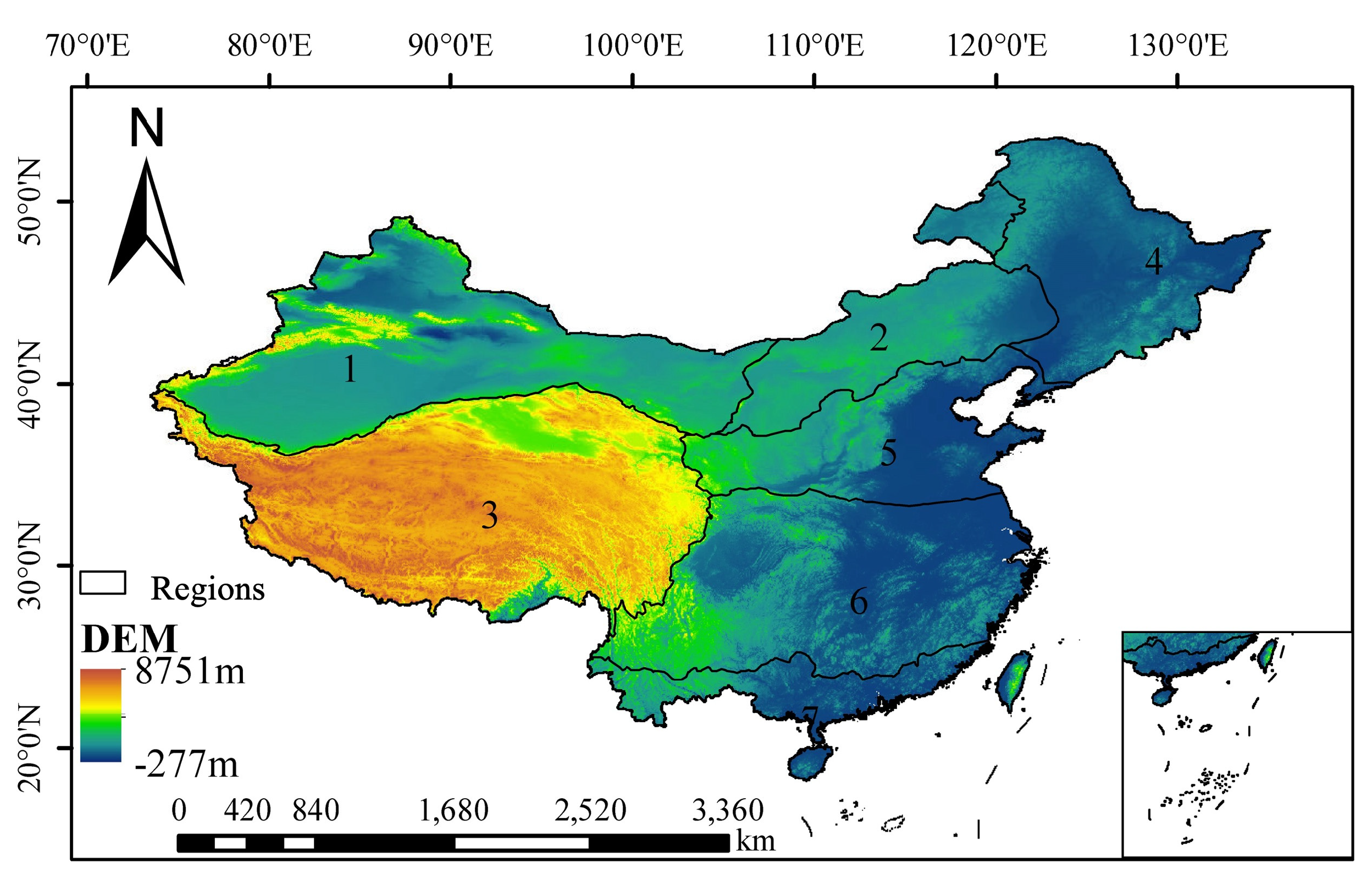
Figure 2.
Schematic diagram of drought patches identification.
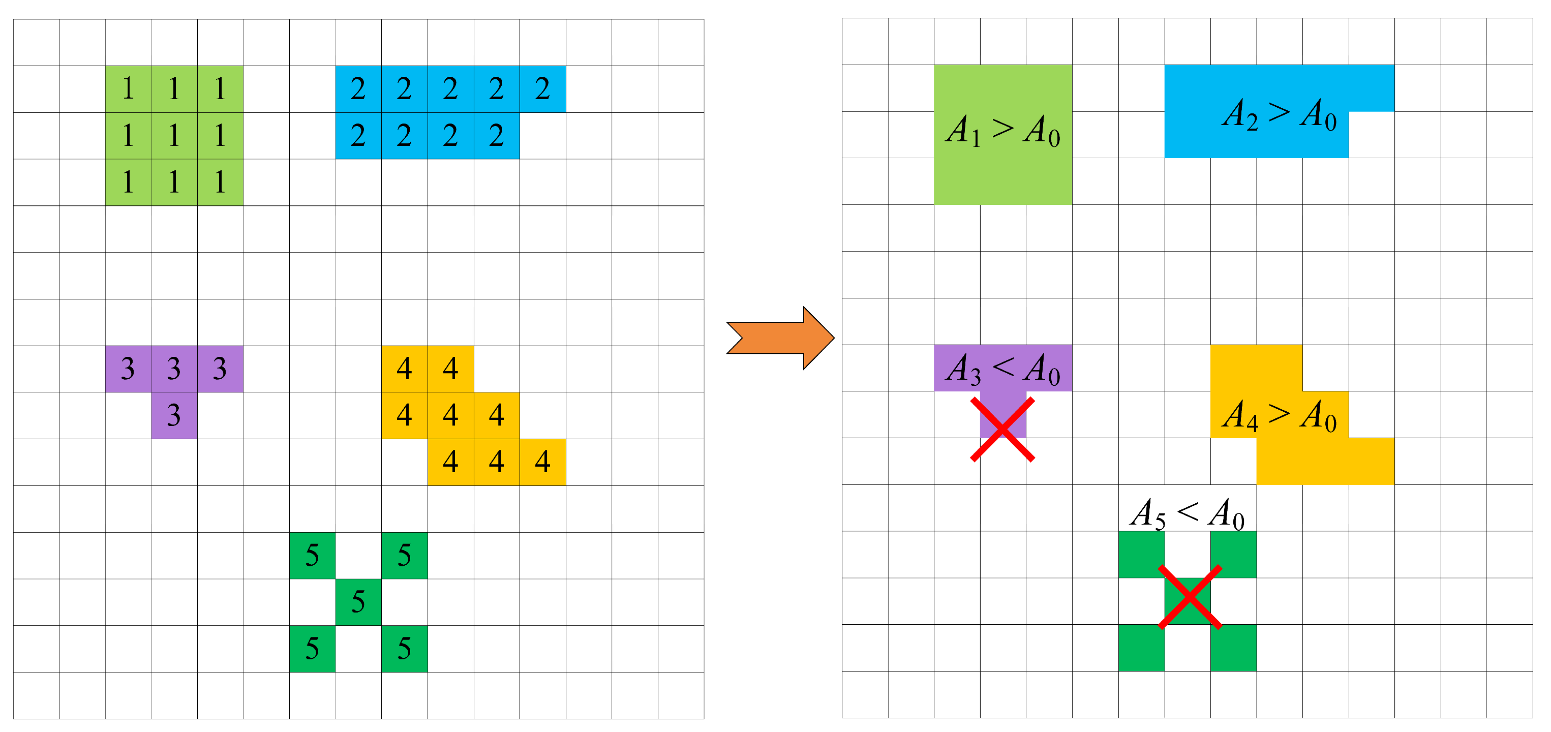
Figure 3.
Schematic diagram of the temporal connection of drought patches.
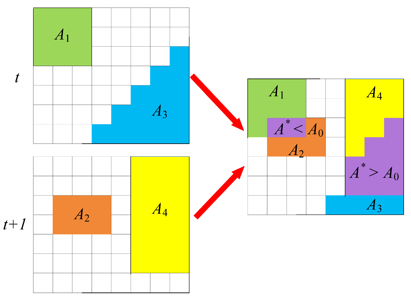
Figure 4.
The variations of annual SZI[CO2] from different sub-regions and China based on multi-model ensemble over 1985–2100 under the SSP2-4.5 and SSP5-8.5 scenarios.
Figure 4.
The variations of annual SZI[CO2] from different sub-regions and China based on multi-model ensemble over 1985–2100 under the SSP2-4.5 and SSP5-8.5 scenarios.
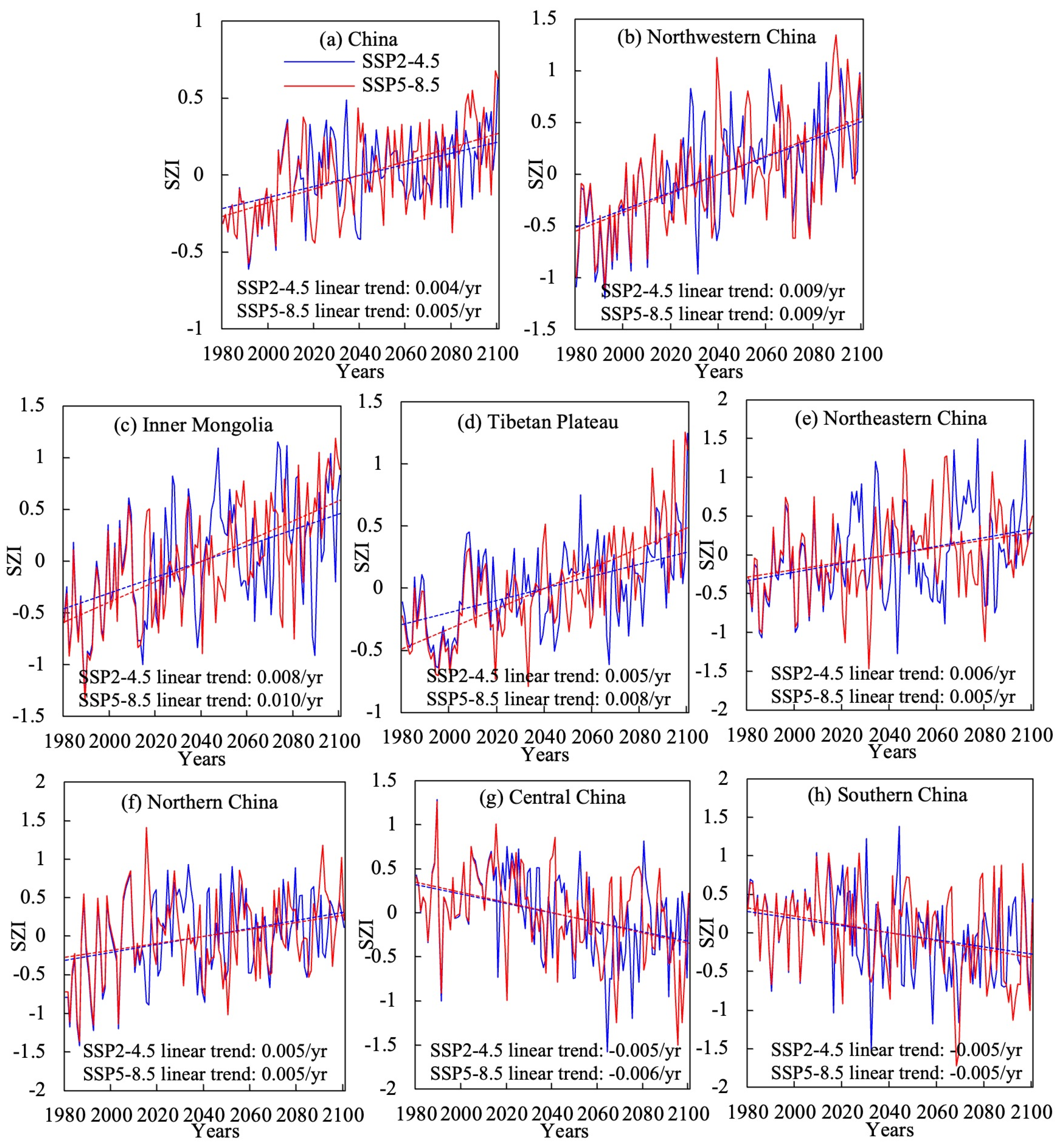
Figure 5.
Annual variations of relative drought area (RDA) in China and seven climatic regions for 1985–2100 under SSP2-4.5 and SSP5-8.5 scenarios.
Figure 5.
Annual variations of relative drought area (RDA) in China and seven climatic regions for 1985–2100 under SSP2-4.5 and SSP5-8.5 scenarios.
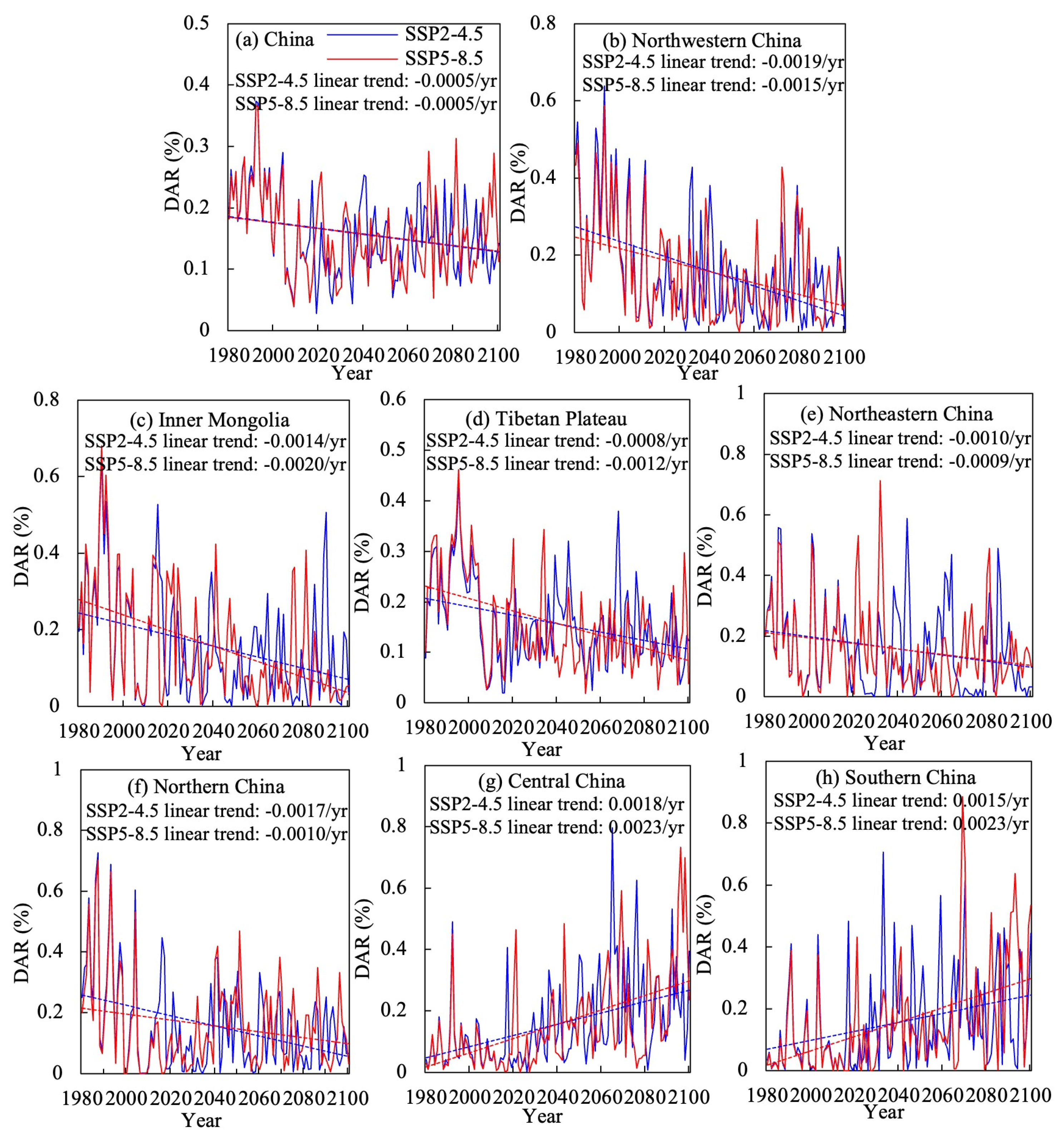
Figure 6.
Spatiotemporal evolution of the No. 474 drought event (2094.08–2097.05) in Central China under the SSP5-8.5 scenario.
Figure 6.
Spatiotemporal evolution of the No. 474 drought event (2094.08–2097.05) in Central China under the SSP5-8.5 scenario.
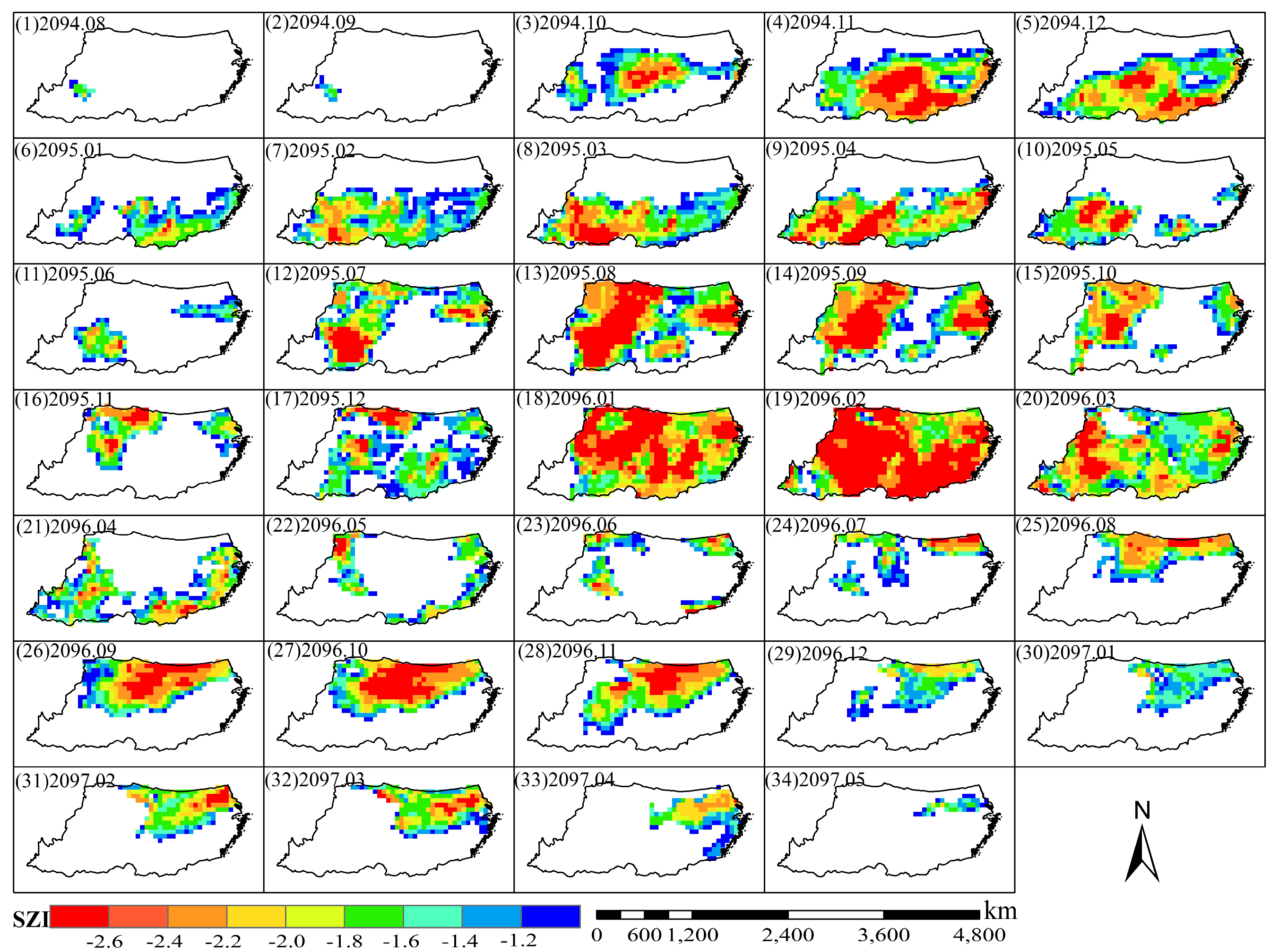
Figure 7.
Migration path of the drought center of the No. 474 drought event (2094.08–2097.05) in Central China under the SSP5-8.5 scenario.
Figure 7.
Migration path of the drought center of the No. 474 drought event (2094.08–2097.05) in Central China under the SSP5-8.5 scenario.
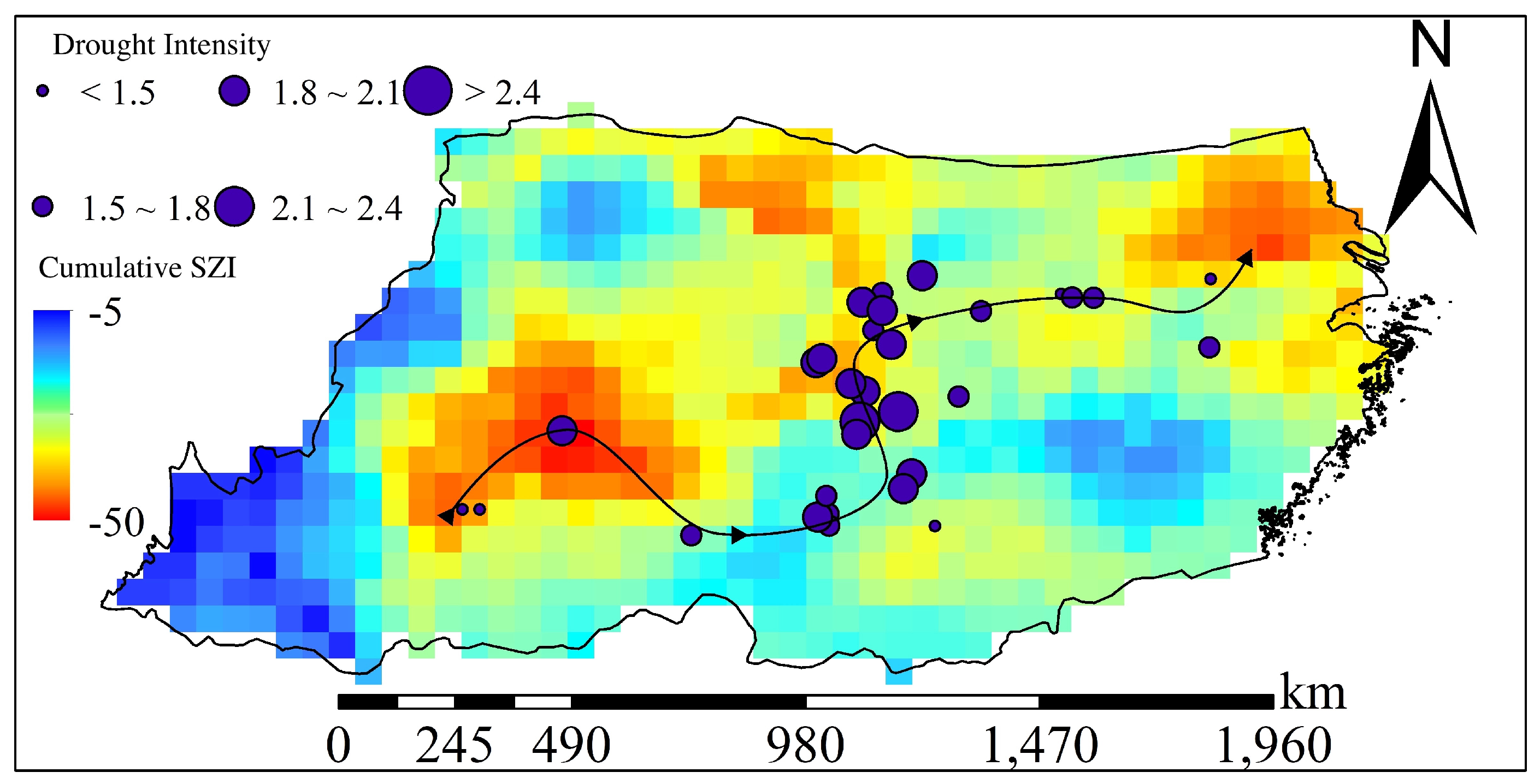
Figure 8.
Figure 8. The bivariate joint occurrence probability of drought duration (month) and area (105 km2) in ‘or’ case and ‘and’ case under SSP2-4.5 and SSP5-8.5 scenarios in 7 climatic regions of China.
Figure 8.
Figure 8. The bivariate joint occurrence probability of drought duration (month) and area (105 km2) in ‘or’ case and ‘and’ case under SSP2-4.5 and SSP5-8.5 scenarios in 7 climatic regions of China.
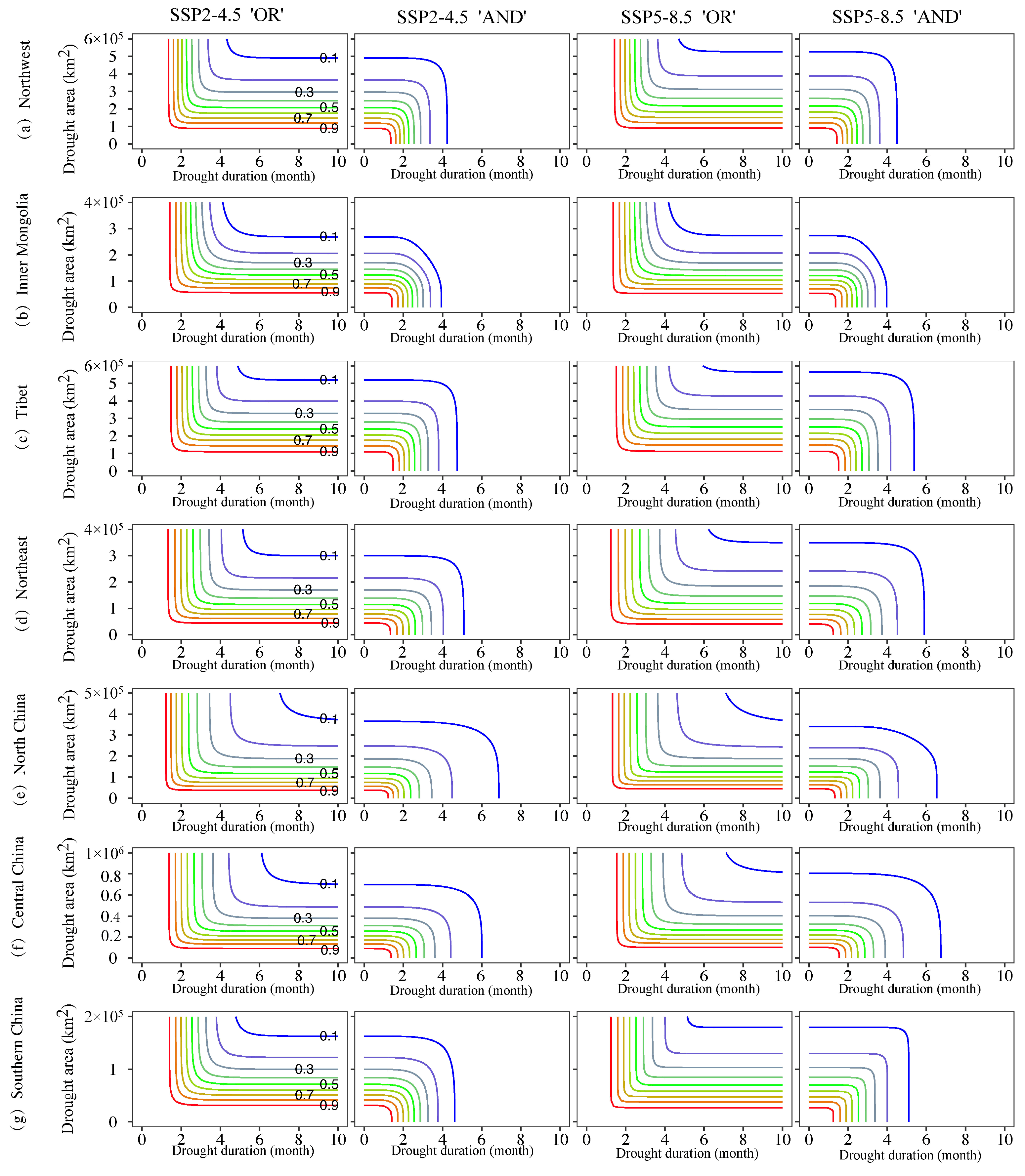
Figure 9.
Figure 9. The trivariate occurrence probability of drought duration (month), drought area (105km2), and drought severity (106 km2 ·month) in ‘or’ case and ‘and’ case under SSP2-4.5 and SSP5-8.5 scenarios in Northwest China.
Figure 9.
Figure 9. The trivariate occurrence probability of drought duration (month), drought area (105km2), and drought severity (106 km2 ·month) in ‘or’ case and ‘and’ case under SSP2-4.5 and SSP5-8.5 scenarios in Northwest China.
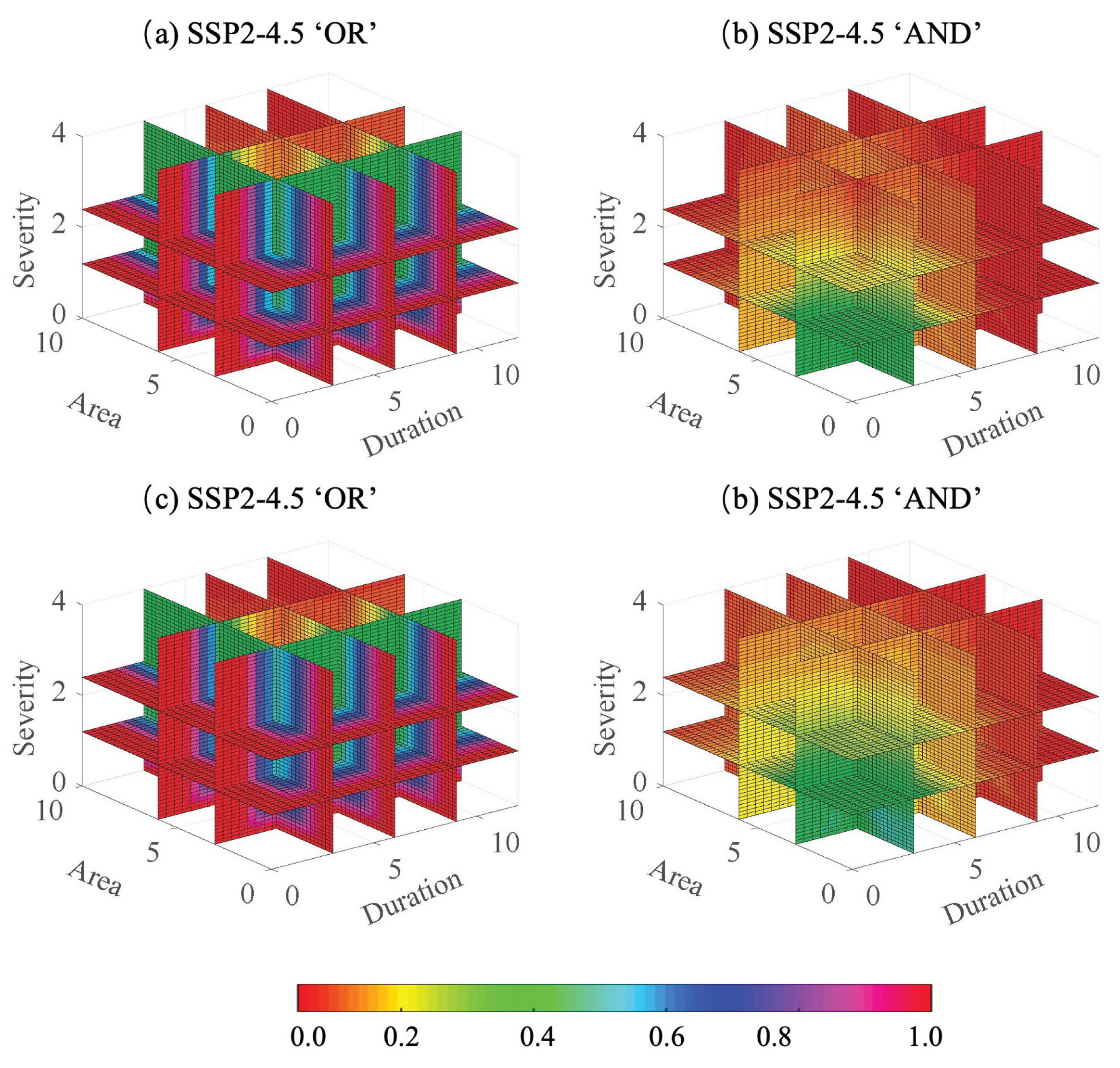

Table 1.
Affiliated institutions and resolutions of 10 GCMs from CMIP6.
| CMIP6 | Country | Resolution (Lat/Lon°) |
|---|---|---|
| ACCESS-ESM-1-5 | Australia | 1.3 × 1.9 |
| BCC-CSM2-MR | China | 2.8 × 2.8 |
| CESM2 | America | 0.9 × 1.3 |
| EC-EARTH3 | Europe | 1.1 × 1.1 |
| GFDL-ESM4 | America | 2.0 × 2.5 |
| HadGEM3-GC31-LL | United Kingdom | 1.3 × 1.9 |
| MIROC6 | Japan | 1.4 × 1.4 |
| MPI-ESM1-2-HR | Germany | 1.9 × 1.9 |
| MRI-ESM2-0 | Japan | 1.1 × 1.1 |
| NorESM2-MM | Norway | 1.9 × 2.5 |
Disclaimer/Publisher’s Note: The statements, opinions and data contained in all publications are solely those of the individual author(s) and contributor(s) and not of MDPI and/or the editor(s). MDPI and/or the editor(s) disclaim responsibility for any injury to people or property resulting from any ideas, methods, instructions or products referred to in the content. |
© 2025 by the authors. Licensee MDPI, Basel, Switzerland. This article is an open access article distributed under the terms and conditions of the Creative Commons Attribution (CC BY) license (http://creativecommons.org/licenses/by/4.0/).
Copyright: This open access article is published under a Creative Commons CC BY 4.0 license, which permit the free download, distribution, and reuse, provided that the author and preprint are cited in any reuse.


