A Study on the Semi-Discrete KP Equation: Bilinear Bäcklund Transformation, Lax Pair and Periodic Solutions

1. Introduction

Discrete integrable systems play a fundamental role in modern mathematical physics, serving as integrable discretizations of continuous soliton equations and providing exact lattice models for nonlinear wave phenomena [1,2,3,4,5,6,7]. The well-known discrete equation called Hirota-Miwa equation [8,9] reads as

$$a_1(a_2-a_3)T_1\left(\tau \right)T_{23}\left(\tau \right)+a_2(a_3-a_1)T_2\left(\tau \right)T_{31}\left(\tau \right)+a_3(a_1-a_2)T_3\left(\tau \right)T_{12}\left(\tau \right)=0,$$

where $\tau$ is a function of discrete variables $n_1$, $n_2$ and $n_3$, $T_i$ is the shift operator defined by $T_i\left(\tau \right)=\tau (n_i+1)$, $T_{ij}=T_i\left(T_j\left(\tau \right)\right)$ and $a_i$ are lattice parameters. A semi-discrete KP (sdKP) equation [8] was obtained by taking a continuous limit from the Hirota-Miwa equation, and its bilinear form is

$$(a_1-a_2)(T_1\left(\tau \right)T_2\left(\tau \right)-T_{12}\left(\tau \right)\tau )+a_1{a}_2{D}_x{T}_1\left(\tau \right)·T_2\left(\tau \right)=0.$$

(1)

The above equation can be expressed as the equivalent form

$$(a_1{a}_2{D}_x{\mathrm{e}}^{{\displaystyle \frac{D_{n_1}-D_{n_2}}{2}}}-(a_1-a_2){\mathrm{e}}^{{\displaystyle \frac{D_{n_1}+D_{n_2}}{2}}}+(a_1-a_2){\mathrm{e}}^{{\displaystyle \frac{D_{n_1}-D_{n_2}}{2}}})\tau ·\tau =0,$$

(2)

where Hirota’s bilinear operators are defined by [11]

$$D_x^m{D}_t^{n}f(x,t)·g(x,t)={\displaystyle \frac{{\partial }^m}{\partial y^m}}{\displaystyle \frac{{\partial }^n}{\partial s^n}}{f(x+y,t+s)g(x-y,t-s)|}_{s=0,y=0}$$

and

$${\mathrm{e}}^{\delta D_n}f\left(n\right)·g\left(n\right)=f(n+\delta )g(n-\delta ).$$

Through the dependent variable transformation $G=-{(ln\tau )}_x$, the bilinear sdKP Equation (2) is rewritten in nonlinear form

$$a_1{a}_2(G_1-G_2)(G_{12}-G_1-G_2+G)+(G_{1x}-G_{2x})=(a_1-a_2)(G_{12}-G_1-G_2+G).$$

(3)

Determinant solutions, including soliton solutions of Equation (3) were obtained in [10], while periodic solutions are also an important part of integrable systems. Nakamura presented a direct approach [12,13] to get multi-periodic wave solutions of nonlinear integrable equations, by using Riemann theta functions [14,15]. This method has been applied to some continuous soliton equations including (1+1) and (2+1) dimensions [16,17,18,19,20]. However, its application to discrete equations remains relatively rare [21,22,23]. The purpose of this paper is to construct periodic solutions of the semi-discrete KP equation and analyze their connection with soliton solutions. This paper is organized as follows. In Section 2, Bäcklund transformations, Lax pair and the nonlinear superposition formula are derived. In Section 3 and 4, the one-periodic solution and the two-periodic solution are obtained, and the asymptotic properties are discussed. Finally, conclusion and discussions are given in Section 5.

2. Bilinear Bäcklund Transformation and the Nonlinear Superposition Formula

The bilinear sdKP Equation (2) has the following bilinear Bäcklund transformation (BT) [24]

$$\begin{array}{ccc}& & D_x\tau ·\tilde{\tau }=\theta \tau ·\tilde{\tau }+{\displaystyle \frac{1}{\lambda }}(a_1-a_2){\mathrm{e}}^{D_{n_2}}\tau ·\tilde{\tau }\hfill \end{array}$$

(4)

$$\begin{array}{ccc}& & {\mathrm{e}}^{-{\displaystyle \frac{D_{n_1}}{2}}}\tau ·\tilde{\tau }=\mu {\mathrm{e}}^{{\displaystyle \frac{D_{n_1}}{2}}}\tau ·\tilde{\tau }+{\displaystyle \frac{1}{\lambda }}{a}_1{a}_2{\mathrm{e}}^{D_{n_2}-{\displaystyle \frac{D_{n_1}}{2}}}\tau ·\tilde{\tau }.\hfill \end{array}$$

(5)

where $\theta$, $\mu$ are arbitrary constants, and $\lambda$ is a nonzero constant. If we take $\tau =1,$$\tilde{\tau }=1+{\mathrm{e}}^{\xi }$, $\xi =rx+p{n}_1+q{n}_2+{\xi }_0$, and substitute $\tau$, $\tilde{\tau }$ in BT (4)-(5), the relationship of parameters p, q and r can be obtained

$$r={\displaystyle \frac{(a_2-a_1)({\mathrm{e}}^p+{\mathrm{e}}^q-{\mathrm{e}}^{p+q}-1)}{a_1{a}_2({\mathrm{e}}^p-{\mathrm{e}}^q)}}.$$

Therefore the function $\tilde{\tau }$ satisfying the above dispersion relation gives one-soliton solution of the sdKP Equation (3), that is

$$G=-{(ln(1+{\mathrm{e}}^{\xi }))}_x.$$

(6)

In addition, a nonlinear superposition formula is derived using the BT as well, and the formula is as follows.

Proposition 1. 

Let ${\tau }_0$ be a solution of Equation (2). Suppose that ${\tau }_1$, ${\tau }_2$ are solutions of Equation (2) given by BT (4)-(5) with a starting solution ${\tau }_0$ and Bäcklund parameters $({\lambda }_1,{\mu }_1,{\theta }_1)$ and $({\lambda }_2,{\mu }_2,{\theta }_2)$ respectively, where $({\lambda }_1,{\mu }_1,{\theta }_1)\ne ({\lambda }_2,{\mu }_2,{\theta }_2)$, ${\tau }_j\ne 0,j=0,1,2$. Then ${\tau }_{12}$ defined by

$${\mathrm{e}}^{{\displaystyle \frac{D_{n_2}}{2}}}{\tau }_0·{\tau }_{12}=C({\lambda }_1{\mathrm{e}}^{-{\displaystyle \frac{D_{n_2}}{2}}}-{\lambda }_2{\mathrm{e}}^{{\displaystyle \frac{D_{n_2}}{2}}}){\tau }_1·{\tau }_2$$

(7)

is a new solution of Equation (2), where C is a non-zero constant.

Starting from the bilinear BT (4)-(5), and using the transformation $\phi ={\displaystyle \frac{\tilde{\tau }}{\tau }}$, we can also get the Lax pair of the sdKP Equation (3) according to the compatibility condition ${\left({\phi }_x\right)}_{n_1+1}={\left({\phi }_{n_1+1}\right)}_x$. The Lax pair is written as follows

$$\begin{array}{ccc}& & {\phi }_x=-\theta \phi -{\displaystyle \frac{1}{\lambda }}(a_1-a_2){\displaystyle \frac{{\tau }_{n_1}^{n_2+1}{\tau }_{n_1}^{n_2-1}}{{\left(\tau \right)}^2}}{\phi }_{n_2-1},\hfill \end{array}$$

(8)

$$\begin{array}{ccc}& & {\phi }_{n_1+1}=\mu \phi +{\displaystyle \frac{1}{\lambda }}{a}_1{a}_2{\displaystyle \frac{{\tau }_{n_1}^{n_2+1}{\tau }_{n_1+1}^{n_2-1}}{{\tau }_{n_1+1}^{n_2}\tau }}{\phi }_{n_1+1}^{n_2-1}.\hfill \end{array}$$

(9)

3. One-Periodic Wave Solution of the sdKP Equation and Its Asymptotic Property

In this part, a one-periodic wave solution of the sdKP Equation (3) is given by Hirota’s method and Riemann theta functions. In this case, the theta function takes the form

$$f=\theta (\eta ,b)=\sum _{n=-\infty }^{+\infty }{\mathrm{e}}^{2\pi in\eta -\pi n^{2}b}$$

(10)

in which $\eta =kx+l{n}_1+w{n}_2+{\eta }_0,\eta \in C$, and b is a positive real constant.

3.1. One-Periodic Wave Solution

In order to get periodic wave solutions, the sdKP Equation (3) needs to be rewritten as another bilinear form

$$(a_1{a}_2{D}_x{\mathrm{e}}^{{\displaystyle \frac{D_{n_1}-D_{n_2}}{2}}}-(a_1-a_2){\mathrm{e}}^{{\displaystyle \frac{D_{n_1}+D_{n_2}}{2}}}+(a_1-a_2){\mathrm{e}}^{{\displaystyle \frac{D_{n_1}-D_{n_2}}{2}}}+c{\mathrm{e}}^{{\displaystyle \frac{D_{n_1}+D_{n_2}}{2}}})\tau ·\tau =0,$$

(11)

where c is a non-zero constant. If the constant c is zero, the above equation degenerates to the original Equation (2). In what follows, we use the notation $D_i=D_{n_i},i=1,2,3$, the Equation (11) can be expressed as the equivalent form

$$\begin{array}{cc}\hfill & \left[a_1{a}_2{D}_{x}sinh{\displaystyle \frac{D_1-D_2}{2}}+(a_1-a_2)(cosh{\displaystyle \frac{D_1-D_2}{2}}-cosh{\displaystyle \frac{D_1+D_2}{2}})\right.\hfill \\ \hfill & \left.+ccosh{\displaystyle \frac{D_1+D_2}{2}})\right]\tau ·\tau =0\hfill \end{array}$$

(12)

Now we take the notation

$$\begin{array}{ccc}\hfill F& =& F\left(D_{x}sinh{\displaystyle \frac{D_1-D_2}{2}},cosh{\displaystyle \frac{D_1-D_2}{2}},cosh{\displaystyle \frac{D_1+D_2}{2}},c\right)\hfill \\ & =& a_1{a}_2{D}_{x}sinh{\displaystyle \frac{D_1-D_2}{2}}+(a_1-a_2)\left(cosh{\displaystyle \frac{D_1-D_2}{2}}-cosh{\displaystyle \frac{D_1+D_2}{2}}\right)\hfill \\ & & +ccosh{\displaystyle \frac{D_1+D_2}{2}},\hfill \end{array}$$

(13)

and Equation (12) is in the simple form $F\tau ·\tau =0$. Then substituting the theta function (10) into the LHS of Equation (12), we get

$$Ff·f=\sum _{m=-\infty }^{+\infty }\tilde{F}\left(m\right){\mathrm{e}}^{2\pi im\eta },$$

(14)

where $\tilde{F}\left(m\right)$ has the following definition

$$\begin{array}{cc}\hfill \tilde{F}\left(m\right)=& \sum _{n=-\infty }^{+\infty }F(2\pi i(2n-m)ksinh\pi i(2n-m)(l-w),cosh\pi i(2n-m)(l-w),\hfill \\ \hfill & cosh\pi i(2n-m)(l+w),c)\times {\mathrm{e}}^{\pi i(n^2+{(m-n)}^2)b}.\hfill \end{array}$$

(15)

By shifting the summation index by $n=n^{\prime }+1$, we have

$$\begin{array}{ccc}\hfill \tilde{F}\left(m\right)& =& \tilde{F}(m-2){\mathrm{e}}^{-2\pi (m-1)b}=\dots \hfill \\ & =& \left\{\begin{array}{cc}\tilde{F}\left(0\right){\mathrm{e}}^{-2\pi n^{2}b/2},\hfill & \mathrm{m}\mathrm{is}\mathrm{even}\hfill \\ \tilde{F}\left(1\right){\mathrm{e}}^{-2\pi (n^2-1)b/2},\hfill & \mathrm{m}\mathrm{is}\mathrm{odd},\hfill \end{array}\right.\hfill \end{array}$$

which implies that if the following equations are satisfied,

$$\tilde{F}\left(0\right)=\tilde{F}\left(1\right)=0$$

(16)

then it shows that $\tilde{F}\left(m\right)=0$ for all $m\in Z$, and thus the theta function (10) satisfies the bilinear sdKP Equation (12). According to Equations (15) and (16), we have

$$\begin{array}{ccc}& & \begin{array}{c}{\displaystyle \sum _{n=-\infty }^{+\infty }}(4\pi a_1{a}_2\mathrm{i}nksinh2\pi in(l-w)+(a_1-a_2)cosh2\pi in(l-w)\hfill \\ -(a_1-a_2)cosh2\pi in(l+w)+c·cosh2\pi in(l+w)){\mathrm{e}}^{-2\pi n^{2}b}=0,\hfill \end{array}\hfill \end{array}$$

(17)

$$\begin{array}{ccc}& & \begin{array}{c}{\displaystyle \sum _{n=-\infty }^{+\infty }}(a_1{a}_2\left(\pi i(2n-1)k\right)sinh\pi i(2n-1)(l-w)\hfill \\ +(a_1-a_2)cosh\pi i(2n-1)(l-w)-(a_1-a_2)cosh\pi i(2n-1)(l-w)\hfill \\ +c·cosh\pi i(2n-1)(l+w)){\mathrm{e}}^{-\pi (2n^2-2n+1)b}=0\hfill \end{array}\hfill \end{array}$$

(18)

We introduce the notation

$$\begin{array}{cc}\hfill \varphi & ={\mathrm{e}}^{-\pi b},a_{11}=\sum _{n=-\infty }^{+\infty }(a_1{a}_{2}4\pi inksinh2\pi in(l-w)){\varphi }^{2n^2},\hfill \\ \hfill a_{12}& =\sum _{n=-\infty }^{+\infty }(cosh2\pi in(l+w){\varphi }^{2n^2},\hfill \\ \hfill a_{21}& =\sum _{n=-\infty }^{+\infty }(2a_1{a}_2\pi i(2n-1)sinh2\pi i(2n-1)(l-w)){\varphi }^{2n^2-2n+1},\hfill \\ \hfill a_{22}& =\sum _{n=-\infty }^{+\infty }(cosh\pi i(2n-1)(l+w){\varphi }^{2n^2-2n+1},\hfill \\ \hfill d_1& =\sum _{n=-\infty }^{+\infty }(a_2-a_1)[cosh2\pi in(l-w)-cosh2\pi in(l+w)]{\varphi }^{2n^2},\hfill \\ \hfill d_2& =\sum _{n=-\infty }^{+\infty }(a_2-a_1)[cosh\pi i(2n-1)(l-w)-cosh2\pi i(2n-1)(l+w)]{\varphi }^{2n^2-2n+1},\hfill \end{array}$$

(19)

Equations (17) and (18) can be written as a system of linear equations about the parameters k and c, i.e.

$$\begin{array}{c}\hfill \left(\begin{array}{cc}{a}_{11}& a_{12}\\ a_{21}& a_{22}\end{array}\right)\left(\begin{array}{c}k\\ c\end{array}\right)=\left(\begin{array}{c}{d}_1\\ d_2\end{array}\right).\end{array}$$

(20)

Hence we get a one-periodic wave solution of the sdKP Equation (3)

$$G=-{(ln\theta (\eta ,b))}_x,$$

(21)

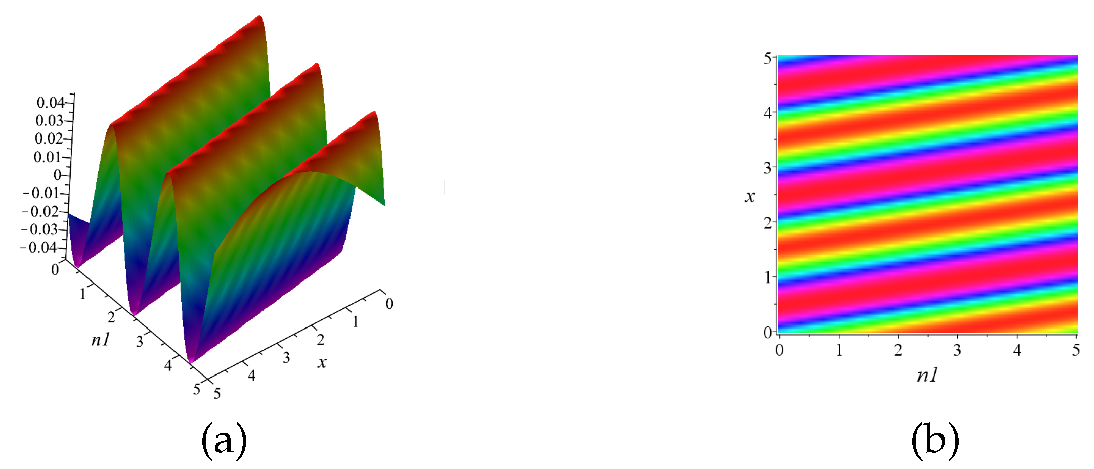
where the theta function $\theta (\eta ,b)$ is given by Equation (10), and the parameters k and c are solved by Equation (20), other parameters l, w, ${\eta }_0$ and b are free, in which l, w and b play a major rule in one periodic wave solution. Here we present the graph of the one-periodic wave solution (21) with the parameter values chosen as $k=1$, $l=0.5$, $w=0.5$ and $n_2=1$.

Figure 1. (a) One-periodic wave solution, (b) Density plot of the one-periodic wave solution.

Figure 1. (a) One-periodic wave solution, (b) Density plot of the one-periodic wave solution.

3.2. Asymptotic Properties of the One-Periodic Wave Solution

Next, we consider the asymptotic properties of the one-periodic wave solution and establish the relationship of soliton solutions and periodic solutions by taking a limit condition. For this purpose, we give the expansions of the matrix $A={\left(a_{ij}\right)}_{2\times 2}$, the vectors ${(d_1,d_2)}^T$ and ${(k,c)}^T$

$$\begin{array}{ccc}& & \left(\begin{array}{cc}{a}_{11}& a_{12}\\ a_{21}& a_{22}\end{array}\right)=A_0+A_1+A_2{\varphi }^2+\dots ,\hfill \\ & & \left(\begin{array}{c}{d}_1\\ d_2\end{array}\right)=D_0+D_1+D_2{\varphi }^2+\dots ,\hfill \\ & & \left(\begin{array}{c}k\\ c\end{array}\right)=X_0+X_1\varphi +X_2{\varphi }^2+\dots ,\hfill \end{array}$$

According to the expression of $a_{ij}$, $d_j$ ($i,j=1,2$) in (19) and expanding these elements to be the sum of $\varphi$, we have

$$\begin{array}{ccc}& & A_0=\left(\begin{array}{cc}0& 1\\ 0& 0\end{array}\right),A_1=\left(\begin{array}{cc}0& 0\\ 4a_1{a}_2\pi isinh\pi i(l-w)& 2cosh\pi i(l+w)\end{array}\right),\hfill \\ & & A_2=\left(\begin{array}{cc}8a_1{a}_2\pi isinh2\pi i(l-w)& 2cosh2\pi i(l+w)\\ 0& 0\end{array}\right),A_3=A_4=\left(\begin{array}{cc}0& 0\\ 0& 0\end{array}\right),\hfill \\ & & A_5=\left(\begin{array}{cc}0& 0\\ 12a_1{a}_2\pi isinh3\pi i(l-w)& 2cosh3\pi i(l+w)\end{array}\right),\dots \hfill \end{array}$$

$$\begin{array}{ccc}& & D_0=\left(\begin{array}{c}0\\ 0\end{array}\right),D_1=\left(\begin{array}{c}0\\ 2(a_2-a_1)(cosh\pi i(l-w)-cosh\pi i(l+w))\end{array}\right),\hfill \\ & & D_2=\left(\begin{array}{c}2(a_2-a_1)(cosh2\pi i(l-w)-cosh2\pi i(l+w))\\ 0\end{array}\right),D_3=D_4=\left(\begin{array}{c}0\\ 0\end{array}\right),\hfill \\ & & D_5=\left(\begin{array}{c}0\\ 2(a_2-a_1)(cosh3\pi i(l-w)-cosh3\pi i(l+w))\end{array}\right),\dots \hfill \end{array}$$

Therefore, we obtain the following result

$$X_0=\left(\begin{array}{c}{k}_0\\ 0\end{array}\right),X_1=\left(\begin{array}{c}0\\ 0\end{array}\right),X_2=\left(\begin{array}{c}{k}_2\\ c_2,\end{array}\right),$$

(22)

where $k_0$ and $c_2$ have the following expression

$$\begin{array}{cc}\hfill k_0& ={\displaystyle \frac{(a_2-a_1)(cosh\pi i(l-w)-cosh\pi i(l+w))}{2a_1{a}_2\pi isinh\pi i(l-w)}},\hfill \\ \hfill c_2& =2(a_2-a_1)[cosh2\pi i(l-w)-cosh2\pi i(l+w)\hfill \\ \hfill & -{\displaystyle \frac{4(cosh\pi i(l-w)-cosh\pi i(l+w\left)\right)sinh2\pi i(l-w)}{sinh\pi i(l-w)}}].\hfill \end{array}$$

(23)

The relation between the periodic wave solution and the one-soliton solution is given by Theorem 1.

Theorem 1. 

If the one-periodic solution of Equation 3 satisfies the following condition

$$k={\displaystyle \frac{r}{2\pi i}},l={\displaystyle \frac{p}{2\pi i}},w={\displaystyle \frac{q}{2\pi i}},{\eta }_0={\displaystyle \frac{{\xi }_0+\pi b}{2\pi i}},$$

(24)

where r, p, q and ${\xi }_0$ are the same as those in expression (6), we have the following asymptotic properties

$$c\to 0,\eta \to {\displaystyle \frac{\xi +\pi b}{2\pi i}},\theta (\eta ,b)\to 1+{\mathrm{e}}^{\xi },\varphi \to 0.$$

Proof. 

Firstly, by using the formula in (22), parameters k and c are written as

$$k=k_0+k_2{\varphi }^2+\dots =o\left(\varphi \right),c=0+c_2{\varphi }^2+\dots =o\left(\varphi \right),$$

(25)

which implies that $c\to 0$. Now we expand the periodic wave function $\theta (\eta ,b)$ in (10) as the form

$$\begin{array}{cc}\hfill \theta (\eta ,b)& =1+(e^{2\pi i\eta }+e^{-2\pi i\eta })\varphi +(e^{4\pi i\eta }+e^{-4\pi i\eta }){\varphi }^4+(e^{6\pi i\eta }+e^{-6\pi i\eta }){\varphi }^9+\dots \hfill \\ & =1+e^{{\eta }^{\prime }}+(e^{-{\eta }^{\prime }}+e^{2{\eta }^{\prime }}){\varphi }^2+(e^{-2{\eta }^{\prime }}+e^{3{\eta }^{\prime }}){\varphi }^6+\dots ,\hfill \end{array}$$

and accordingly, ${\eta }^{\prime }$ has the following form

$${\eta }^{\prime }=2\pi i\eta -\pi b=2\pi ikx+2\pi il{n}_1+2\pi iw{n}_2+2\pi i{\eta }_0-\pi b=rx+p{n}_1+q{n}_2+{\xi }_0.$$

According to the expression of k in (25), we have

$${\eta }^{\prime }\to k_{0}x+p{n}_1+q{n}_2+{\xi }_0,\varphi \to 0,$$

where the expression of $k_0$ is the same as the expression of r in the one-soliton solution (6). Thus we obtain

$$\theta (\eta ,b)\to 1+{\mathrm{e}}^{\xi },\varphi \to 0.$$

which shows that one periodic wave solution tends to the one soliton solution (6) under the condition $\varphi \to 0$. □

4. Two-Periodic Wave Solution of the sdKP Equation and Its Asymptotic Property

In this section, the two-periodic wave solution is considered and in the case $N=2$, the Riemann theta function is defined as the following series

$$\theta (\eta ,B)=\theta ({\eta }_1,{\eta }_2,B)=\sum _{s=-\infty }^{+\infty }{\mathrm{e}}^{2\pi i<\eta ,s>-\pi <Bs,s>},$$

(26)

where $s={(s_1,s_2)}^T\in Z^2$, $\eta ={({\eta }_1,{\eta }_2)}^T\in C^2$, ${\eta }_j=k_{j}x+l_j{n}_1+w_j{n}_2+{\eta }_{0j},j=1,2$, the symbols $<,>$ denote the inner product of vectors, and B is a positive-definite and real-valued symmetric matrix, which can take the form

$$B=\left(\begin{array}{cc}{b}_{11}& b_{12}\\ b_{21}& b_{22}\end{array}\right),b_{11}>0,b_{22}>0,b_{11}{b}_{22}-b_{12}{b}_{21}>0.$$

4.1. Two-Periodic Wave Solution

In order to obtain the two-periodic solution, the theta function is substituted into the LHS of Equation (12) and the following result is derived

$$\begin{array}{cc}\hfill & F\theta (\eta ,B)·\theta (\eta ,B)=\sum _{s=-\infty }^{+\infty }\sum _{s^{\prime }=-\infty }^{+\infty }{\mathrm{e}}^{2\pi i<\eta ,s^{\prime }>-\pi <Bs,s^{\prime }>}\hfill \\ \hfill & =\sum _{s=-\infty }^{+\infty }\sum _{s^{\prime }=-\infty }^{+\infty }[a_1{a}_{2}2\pi i<s-s^{\prime },k>sinh\pi i<s-s^{\prime },l-w>\hfill \\ \hfill & +(a_1-a_2)cosh\pi i<s-s^{\prime },l-w>+(c+a_2-a_1)cosh\pi i<s-s^{\prime },l+w>]\hfill \\ \hfill & \times {\mathrm{e}}^{2\pi i<\eta ,s+s^{\prime }>-\pi <BS,s>-\pi <B{s}^{\prime },s^{\prime }>}\hfill \\ \hfill & \stackrel{s^{\prime }=m-s}{=}\sum _{m=-\infty }^{+\infty }\sum _{s=-\infty }^{+\infty }[a_1{a}_{2}2\pi i<2s-m,k>sinh\pi i<2s-m,l-w>\hfill \\ \hfill & +(a_1-a_2)cosh\pi i<2s-m,l-w>\hfill \\ \hfill & +(c+a_2-a_1)cosh\pi i<2s-m,l+w>]{\mathrm{e}}^{2\pi i<\eta ,m>-\pi <BS,s>-\pi <B(m-s),(m-s)>}\hfill \\ \hfill & =\sum _{m=-\infty }^{+\infty }\overline{F}(m_1,m_2)\times {\mathrm{e}}^{2\pi i<\eta ,m>}\hfill \end{array}$$

(27)

where $s^{\prime }={(s_1^{\prime },s_2^{\prime })}^T$, $k={(k_1,k_2)}^T$, $l={(l_1,l_2)}^T$, $w={(w_1,w_2)}^T$. In the above formula, the notation $\overline{F}(m_1,m_2)$ is defined by

$$\begin{array}{cc}\hfill \overline{F}(m_1,m_2)& =\sum _{s=-\infty }^{+\infty }[a_1{a}_{2}2\pi i<2s-m,k>sinh\pi i<2s-m,l-w>\hfill \\ \hfill & +(a_1-a_2)cosh\pi i<2s-m,l-w>\hfill \\ \hfill & +(c+a_2-a_1)cosh\pi i<2s-m,l+w>]\hfill \\ \hfill & \times {\mathrm{e}}^{-\pi <Bs,s>-\pi <B(m-s),(m-s)>}.\hfill \end{array}$$

(28)

Letting the summation index $s_j=s_j^{\prime }+{\delta }_{jl}$ where ${\delta }_{jl}$ is the Kronecker delta, formula (28) then has the form

$$\begin{array}{cc}\hfill \overline{F}(m_1,m_2)& =\sum _{s=-\infty }^{+\infty }F(2\pi i\left(\sum _{j=1}^2(2s_j^{\prime }-(m_j-2{\delta }_{jl}))\right)sinh\left(\pi i\sum _{j=1}^2(2s_j^{\prime }-(m_j-2{\delta }_{jl}))\right),\hfill \\ \hfill & cosh\left(\pi i\sum _{j=1}^2(2s_j^{\prime }-(m_j-2{\delta }_{jl}))(l_j-w_j)\right),cosh\left(\pi i\sum _{j=1}^2(2s_j^{\prime }-(m_j-2{\delta }_{jl}))(l_j+w_j)\right),c)\hfill \\ \hfill & \times {\mathrm{e}}^{-\pi <Bs,s>-\pi <B(m-s),(m-s)>}.\hfill \\ \hfill & =\left\{\begin{array}{cc}\overline{F}(m_1-2,m_2){\mathrm{e}}^{-\pi [2(b_{11}{m}_1+b_{12}{m}_2)-2b_{11}]},\hfill & l=1\hfill \\ \overline{F}(m_1,m_2-2){\mathrm{e}}^{-\pi [2(b_{12}{m}_1+b_{22}{m}_2)-2b_{22}]},\hfill & l=2\hfill \end{array}.\right.\hfill \end{array}$$

The above result indicates that $\overline{F}(m_1,m_2),(m_1,m_2)\in Z^2$ is entirely determined by $\overline{F}(0,0)$, $\overline{F}(0,1)$, $\overline{F}(1,0)$ and $\overline{F}(1,1)$. Hence, if the following four equations are satisfied

$$\overline{F}(0,0)=\overline{F}(0,1)=\overline{F}(1,0)=\overline{F}(1,1)=0,$$

(29)

then $\overline{F}(m_1,m_2)=0,(m_1,m_2)\in Z^2,$ so $F\theta (\eta ,B)·\theta (\eta ,B)=0$. That is, $\theta (\eta ,B)$ is an exact solution of Equation (12). Next by adopting the following notations

$$\begin{array}{cc}& M=(a_{j1},a_{j2},a_{j3}),j=1,2,3,4,d={(d_1,d_2,d_3,d_4)}^T\hfill \\ & a_{j1}=2\pi i{a}_1{a}_2\sum _{s_1,s_2\in Z^2}(2s_1-r_1^j)sinh\pi i<2s-r^j,l-w>{ϵ}_j(s_1,s_2)\hfill \\ & a_{j2}=2\pi i{a}_1{a}_2\sum _{s_1,s_2\in Z^2}(2s_2-r_2^j)sinh\pi i<2s-r^j,l-w>{ϵ}_j(s_1,s_2)\hfill \\ & a_{j3}=\sum _{s_1,s_2\in Z^2}(2s_1-r_1^j)cosh\pi i<2s-r^j,l-w>{ϵ}_j(s_1,s_2)\hfill \\ & d_j=(a_2-a_1)\sum _{s_1,s_2\in Z^2}[cosh\pi i<2s-r^j,l-w>-cosh\pi i<2s-r^j,l+w>]{ϵ}_j(s_1,s_2)\hfill \\ & {\varphi }_1={\mathrm{e}}^{-\pi b_{11}},{\varphi }_2={\mathrm{e}}^{-\pi b_{22}},{\varphi }_3={\mathrm{e}}^{-2\pi b_{12}},\hfill \\ & {ϵ}_j(s_1,s_2)={\varphi }_1^{s_1^2+{(s_1-r_i^j)}^2}{\varphi }_2^{s_2^2+{(s_2-r_2^j)}^2}{\varphi }_3^{s_1{s}_2+(s_1-r_1^j)(s_2-r_2^j)},\hfill \\ & r^1=(0,0),r^2=(0,1)r^3=(1,0)r^4=(1,1),r^j=(r_1^j,r_2^j),j=1,2,3,4,\hfill \end{array}$$

Equation (29) can be written as the following system

$$M{(k_1,k_2,c)}^T=d.$$

(30)

Therefore, we obtain a two-periodic wave solution of Equation (3)

$$u=-{(ln\theta (\eta ,B))}_x,$$

(31)

where the parameters $\theta (\eta ,B)$, $k_1$, $k_2$, c and $b_{12}$ are determined by (26) and (30), while other parameters $l_1$, $l_2$, $w_1$, $w_2$, $b_{11}$ and $b_{22}$ are free, which play an important role in the two-periodic wave solution.

4.2. Asymptotic Properties of the Two-Periodic Wave Solution

In what follows, we further analyze the asymptotic properties of the two-periodic wave solution (31), and establish the relation between the two-periodic wave and the two-soliton wave [23]. In much the same way as in Theorem 1, we first give the expansions of the matrix M and d in (30)

$$\begin{array}{cc}\hfill & M=\left(\begin{array}{ccc}0& 0& 1\\ 0& 0& 0\\ 0& 0& 0\\ 0& 0& 0\end{array}\right)+\left(\begin{array}{ccc}0& 0& 1\\ 0& 0& 0\\ 4\pi i{a}_1{a}_{2}sinh\pi i(l_1-w_1)& 0& 2cosh\pi i(l_1-w_1)\\ 0& 0& 0\end{array}\right){\varphi }_1\hfill \\ \hfill & +\left(\begin{array}{ccc}0& 0& 0\\ 0& 4\pi i{a}_1{a}_{2}sinh\pi i(l_2-w_2)& 2cosh\pi i(l_2-w_2)\\ 0& 0& 0\\ 0& 0& 0\end{array}\right){\varphi }_2\hfill \\ \hfill & +\left(\begin{array}{ccc}8\pi i{a}_1{a}_{2}sinh2\pi i(l_1-w_1)& 0& 2cosh2\pi i(l_1-w_1)\\ 0& 0& 0\\ 0& 0& 0\\ 0& 0& 0\end{array}\right){\varphi }_1^2\hfill \\ \hfill & +\left(\begin{array}{ccc}0& 8\pi i{a}_1{a}_{2}sinh2\pi i(l_2-w_2)& 2cosh2\pi i(l_2-w_2)\\ 0& 0& 0\\ 0& 0& 0\\ 0& 0& 0\end{array}\right){\varphi }_2^2\hfill \\ \hfill & +\left(\begin{array}{ccc}0& 0& 0\\ 0& 0& 0\\ 0& 0& 0\\ m_1& m_2& m_3\end{array}\right){\varphi }_1{\varphi }_2+o\left({\varphi }_1^m{\varphi }_2^j\right),m+j\ge 2,\hfill \end{array}$$

(32)

in which

$$\begin{array}{cc}\hfill & m_1=4\pi i{a}_1{a}_2[{\varphi }_{3}sinh\pi i(l_1-w_1+l_2-w_2)+sinh\pi i(l_1-w_1-l_2+w_2)],\hfill \\ \hfill & m_2=4\pi i{a}_1{a}_2[{\varphi }_{3}sinh\pi i(l_1-w_1+l_2-w_2)+sinh\pi i(l_2-w_2-l_1+w_1)],\hfill \\ \hfill & m_3=2[{\varphi }_{3}cosh\pi i(l_1-w_1+l_2-w_2)+cosh\pi i(l_1-w_1-l_2+w_2)],\hfill \end{array}$$

and

$$\begin{array}{ccc}& & \begin{array}{cc}& d=\left(\begin{array}{c}0\\ 0\\ 0\\ 0\end{array}\right)+\left(\begin{array}{c}0\\ 0\\ d_1\\ 0\end{array}\right){\varphi }_1+\left(\begin{array}{c}0\\ d_2\\ 0\\ 0\end{array}\right){\varphi }_2\hfill \\ & +\left(\begin{array}{c}{d}_3\\ 0\\ 0\\ 0\end{array}\right){\varphi }_1^2+\left(\begin{array}{c}{d}_4\\ 0\\ 0\\ 0\end{array}\right){\varphi }_2^2+\left(\begin{array}{c}0\\ 0\\ 0\\ d_5\end{array}\right){\varphi }_1{\varphi }_2+o\left({\varphi }_1^m{\varphi }_2^j\right),\hfill \end{array}\hfill \\ & & \begin{array}{cc}& d_1=2(a_2-a_1)[cosh\pi i(l_1-w_1)-cosh\pi i(l_1+w_1)],\hfill \\ & d_2=2(a_2-a_1)[cosh\pi i(l_2-w_2)-cosh\pi i(l_2+w_2)],\hfill \\ & d_3=2(a_2-a_1)[cosh2\pi i(l_1-w_1)-cosh2\pi i(l_1+w_1)],\hfill \\ & d_4=2(a_2-a_1)[cosh2\pi i(l_2-w_2)-cosh2\pi i(l_2+w_2)],\hfill \\ & d_5=2(a_2-a_1)[{\varphi }_{3}cosh\pi i(l_1-w_1+l_2-w_2)+cosh\pi i(l_1-w_1-l_2+w_2)\hfill \\ & -{\varphi }_{3}cosh\pi i(l_1+w_1+l_2+w_2)-cosh\pi i(l_1+w_1-l_2-w_2)].\hfill \end{array}\hfill \end{array}$$

(33)

We assume that the solution of system (30) has the following form

$$\begin{array}{cc}\hfill \left(\begin{array}{c}{k}_1\\ k_2\\ c\end{array}\right)& =\left(\begin{array}{c}{k}_{10}\\ k_{20}\\ c_0\end{array}\right)+\left(\begin{array}{c}{k}_{11}\\ k_{21}\\ c_1\end{array}\right){\varphi }_1+\left(\begin{array}{c}{k}_{12}\\ k_{22}\\ c_2\end{array}\right){\varphi }_2+\left(\begin{array}{c}{k}_{13}\\ k_{23}\\ c_3\end{array}\right){\varphi }_1^2+\left(\begin{array}{c}{k}_{14}\\ k_{24}\\ c_4\end{array}\right){\varphi }_2^2\hfill \\ \hfill & +\left(\begin{array}{c}{k}_{15}\\ k_{25}\\ c_5\end{array}\right){\varphi }_1{\varphi }_2+o\left({\varphi }^m{\varphi }^j\right),m+j\ge 2,\hfill \end{array}$$

(34)

then the relation of the two-periodic solution and the two-soliton solution is given as follows.

Theorem 2. 

If the two-periodic solution in the formula (31) satisfies the following condition

$$k_j={\displaystyle \frac{r_j}{2\pi i}},l_j={\displaystyle \frac{p_j}{2\pi i}},w_j={\displaystyle \frac{q_j}{2\pi i}},{\eta }_{0j}={\displaystyle \frac{{\xi }_{0j}+\pi b_{jj}}{2\pi i}},j=1,2,$$

(35)

where $r_j$, $p_j$, $q_j$ and ${\xi }_{0j}$ are the same as those in the two-soliton solution, we have the following asymptotic properties

$$c\to 0,{\eta }_j\to {\displaystyle \frac{{\xi }_j+\pi b_{jj}}{2\pi i}},\theta ({\eta }_1,{\eta }_2,B)\to 1+{\mathrm{e}}^{{\xi }_1}+{\mathrm{e}}^{{\xi }_2}+A_{12}{\mathrm{e}}^{{\xi }_1+\xi 2},{\varphi }_1,{\varphi }_2\to 0,$$

where $A_{12}={\mathrm{e}}^{-2\pi b_{12}}$.

Proof. 

Substituting formulae (32)-(34) into the system (30), we get the following equalities

$$\begin{array}{cc}& k_j=k_{j0}+o\left({\varphi }_i{\varphi }_2\right),j=1,2,c=c_3{\varphi }_1^2+c_3{\varphi }_2^2+o\left({\varphi }_1^2{\varphi }_2^2\right),\hfill \\ & {\mathrm{e}}^{-2\pi b_{12}}={\displaystyle \frac{4\pi a_1{a}_2(k_{20}-k_{10})sinh\pi ({\widehat{l}}_1-{\widehat{l}}_2)+2(a_2-a_1)(cosh\pi i({\widehat{l}}_1-{\widehat{l}}_2)-cosh\pi i({\widehat{w}}_1-{\widehat{w}}_2)}{4\pi a_1{a}_2(k_{20}+k_{10})sinh\pi ({\widehat{l}}_1+{\widehat{l}}_2)+2(a_2-a_1)(cosh\pi i({\widehat{l}}_1+{\widehat{l}}_2)-cosh\pi i({\widehat{w}}_1+{\widehat{w}}_2))}},\hfill \end{array}$$

where

$$\begin{array}{cc}& k_{j0}={\displaystyle \frac{(a_2-a_1)(cosh\pi i{\widehat{l}}_j-cosh\pi i{\widehat{w}}_j)}{2a_1{a}_2\pi isinh\pi i{\widehat{l}}_j}},c_3={\displaystyle \frac{sinh\pi i{\widehat{l}}_1}{2sinh2\pi i{\widehat{l}}_1}},c_4={\displaystyle \frac{sinh\pi i{\widehat{l}}_2}{2sinh2\pi i{\widehat{l}}_2}},\hfill \end{array}$$

and ${\widehat{l}}_j=l_j-w_j$, ${\widehat{w}}_j=l_j+w_j$, then we have $c\to 0$ as ${\varphi }_1,{\varphi }_2\to 0$. Also, as in the Theorem 1, we expand the theta function $\theta ({\eta }_1,{\eta }_2,B)$ in (26) as the form

$$\begin{array}{cc}\hfill \theta ({\eta }_1,{\eta }_2,B)& =1+({\mathrm{e}}^{2\pi i{\eta }_1}+{\mathrm{e}}^{-2\pi i{\eta }_1}){\varphi }_1+({\mathrm{e}}^{2\pi i{\eta }_2}+{\mathrm{e}}^{-2\pi i{\eta }_2}){\varphi }_2+\dots \hfill \\ & +({\mathrm{e}}^{2\pi i({\eta }_1+{\eta }_2)}+{\mathrm{e}}^{-2\pi i({\eta }_1+{\eta }_2)}){\mathrm{e}}^{-2\pi b_{12}}{\varphi }_1{\varphi }_2+\dots \hfill \\ & =1+{\mathrm{e}}^{{\widehat{\eta }}_1}+{\mathrm{e}}^{{\widehat{\eta }}_2}+{\mathrm{e}}^{{\widehat{\eta }}_1+{\widehat{\eta }}_2-2\pi b_{12}}+{\mathrm{e}}^{-{\widehat{\eta }}_1}{\varphi }_1^2+{\mathrm{e}}^{-{\widehat{\eta }}_2}{\varphi }_2^2+{\mathrm{e}}^{-{\widehat{\eta }}_1-{\widehat{\eta }}_2-2\pi b_{12}}{\varphi }_1^2{\varphi }_2^2+\dots ,\hfill \end{array}$$

in which ${\widehat{\eta }}_j=2\pi i{\eta }_j-\pi b_{jj},j=1,2$. In this case,

$${\widehat{\eta }}_j=2\pi i{k}_{j}x+2\pi i{l}_j{n}_1+2\pi i{w}_j{n}_2+2\pi i{\eta }_{0j}-\pi b_{jj}=r_{j}x+p_j{n}_1+q_j{n}_2+{\xi }_{0j}.$$

According to expressions of $k_j$ and ${\varphi }_3$ as mentioned above, we obtain

$${\widehat{\eta }}_j\to {\xi }_j,\theta ({\eta }_1,{\eta }_2,B)\to 1+{\mathrm{e}}^{{\xi }_1}+{\mathrm{e}}^{{\xi }_2}+A_{12}{\mathrm{e}}^{{\xi }_1+{\xi }_2},{\varphi }_1,{\varphi }_2\to 0,\mathrm{where}{A}_{12}=e^{-2\pi b_{12}}.$$

Therefore, the two-periodic solution tends to a two-soliton solution as ${\varphi }_1,{\varphi }_2\to 0$.

□

5. Conclusions and Discussions

In this paper, we focus on a semi-disceret KP Equation (3) generated by the Hirota-Miwa equation. Its bilinear Bäcklund transformation, Lax pair and nonlinear superposition formula are given. More importantly, using this superposition principle we successfully constructed one-periodic wave solution (21) and two-periodic wave solution (31) which are expressed in terms of Riemann theta functions. Then, one-soliton and two-soliton solutions emerge as natural degenerations by taking appropriate limits of the parameters in the periodic solutions. However, for higher-order periodic solutions, such as the three-periodic wave solution, the associated system of equations for the parameters becomes overdetermined, making it difficult to find exact analytical solutions. Therefore, alternative approaches are needed to obtain such higher-order solutions. For instance, numerical algorithms have been employed in the literature (e.g., in Refs. [19] and [25]) to compute three-periodic solutions for KdV-type and Toda-type equations. In our future work, we will explore the application of numerical methods to simulate three-periodic wave solutions of the semi-discrete KP equation, aiming to gain further insight into its complex nonlinear dynamics. Furthermore, beyond solitons and periodic solutions, integrable systems admit a variety of other important exact solution types including lump solutions and rogue waves. Therefore, another promising direction is to investigate the structure and dynamics of such novel exact solutions for this equation.

References

- Bruschi, M.; Manakov, S. V.; Ragnisco, O.; Levi, D. The nonabelian Toda lattice-discrete analogue of the matrix Schrödinger spectral problem. J. Math. Phys. 1980, 21(2), 2749–2753. [Google Scholar] [CrossRef]
- Levi, D.; Ragnisco, O.; Bruschi, M. Extension of the Zakharov-Shabat generalized inverse method to solve differential-difference and difference-difference equations. Nuovo Cimento A 1980, 58(1), 56–66. [Google Scholar] [CrossRef]
- Takahashi, D. ; Matsukidaira,J. On discrete soliton equations related to cellular automata, Phys. Lett. A, 1995, 209, 184–188. [Google Scholar]
- Hirota, R.; Ohta, Y. Discretization of the new type of soliton equations, J. phys. Soc. Jpn., 2007, 76, 034001. [Google Scholar] [CrossRef]
- Nagai, H.; Ohta, Y.; Hirota, R. Discrete and ultradiscrete periodic phase soliton equations, 2019, 88, 034001.
- Hirota, R. Discrete analogue of a generalized Toda equation. J. Phys. Soc. Jpn., 1981, 50, 3785–3791. [Google Scholar] [CrossRef]
- Amjad, Z.; Haider, B.; Ma, W.X. Integrable discretization and multi-soliton solutions of negative order AKNS equation, 2024, 23(suppl.1), 280.
- Miwa, T. On Hirota’s difference equations. Proc. Japan Acad. A Math. Sci., 1982, 58(1), 9-12.
- Date, E.; Jimbo, M.; Miwa, T. Method for generating discrete solution equations. J. Phys. Soc. Jpn., 1982, 51, 4116–4124. [Google Scholar] [CrossRef]
- Li, C.X.; Lafortune, S.; Shen, S.F. A semi-discrete Kadomtsev-Petviashvili equation and its coupled integrable system. J. Math. Phys. 2017, 57, 053503:1–9. [Google Scholar] [CrossRef]
- Hirota, R. The Direct Method in Soliton Theory. Cambridge University Press, 2004.
- Nakamura, A. A direct method of calculating periodic wave solutions to nonlinear evolution equations. I. exact two-periodic wave solution. J.Phy.Soc.Jpn, 1979, 47(5), 1701-1705.
- Nakamura, A. A direct method of calculating periodic-wave solutions to nonlinear evolution equations. II. exact I-periodic and 2-periodic wave solutions of the coupled bilinear equations, J. Phys. Soc. Jpn. 1980, 48, 1365–1370. [Google Scholar]
- Whittaker, E.T.; Watson, G.N. Acourse of modern analysis. (Cambridge Univ. Press, Cambride), 1935.
- Bellman, R. A brief introduction to theta functions. (Rinehart,R; Winston), Newyork, 1961.
- Hirota, R.; Masaaki, I. A direct approach to multi-periodic wave solutions to nonlinear evolution equations. J. Phys. Soc. Jpn. 1981, 50(1), 338–342. [Google Scholar] [CrossRef]
- Fan, E.G. Quasi-periodic waves and an asymptotic property for the asymmetrical Nizhnik-Novikov-Veselov equation, J. Phys. A: Math. Theor. 2009, 42, 095206. [Google Scholar] [CrossRef]
- Ma, W.X.; Zhou, R.G.; Gao, L. Exact one-periodic and two-periodic wave solutions to Hirota bilinear equations in (2+1)dimensions, Modern Phys. Lett. A 2009, 24, 1677–1688. [Google Scholar]
- Zhang, Y.N.; Hu, X.B.; Sun, J.Q. A numerical study of the 3-periodic wave solutions to KdV-type equations. J. Comp. Phys. 2018, 355, 566–581. [Google Scholar] [CrossRef]
- Wei, L. Multiple periodic-soliton solutions to Kadomtsev-Petviashvili equation, Appl. Math. Comp., 2011, 218, 368–375. [Google Scholar]
- Hon, Y.C.; Fan, E.G.; Qin, Z.Y. A kind of explicit quasi-periodic solution and its limit for the Toda lattice equation, Modern Phys. Lett. B, 2008, 22, 547–553. [Google Scholar]
- Luo, L. Exact periodic wave solutions for the differntial-difference KP equation, Reports on mathematical physics, 2010, 66(3), 403-417.
- Wu, G.C.; Xia, T.C. Uniformly constructing exact discrete soliton solutions and periodic solutions to differential-difference equations, Comput. Math. Appl., 2009, 58, 2351–2354. [Google Scholar]
- Wan, L.S. Nonlinear superposition formula of a semi-discrete KP equation and its exact solutions (master’s thesis), Capital Normal University, Beiing, China, 2024.
- Zhang, Y.N.; Hu, X.B.; Sun, J.Q. A numerical study of the 3-periodic wave solutions to Toda-type equations, Comm. Comp. Phys. 2019, 26(2), 579–598. [Google Scholar]
Disclaimer/Publisher’s Note: The statements, opinions and data contained in all publications are solely those of the individual author(s) and contributor(s) and not of MDPI and/or the editor(s). MDPI and/or the editor(s) disclaim responsibility for any injury to people or property resulting from any ideas, methods, instructions or products referred to in the content. |
© 2025 by the authors. Licensee MDPI, Basel, Switzerland. This article is an open access article distributed under the terms and conditions of the Creative Commons Attribution (CC BY) license (http://creativecommons.org/licenses/by/4.0/).
Copyright: This open access article is published under a Creative Commons CC BY 4.0 license, which permit the free download, distribution, and reuse, provided that the author and preprint are cited in any reuse.