1. Introduction
Interconnection networks are critical for high-performance computing (HPC) systems because they directly impact performance metrics such as latency, bandwidth, and scalability. Among various topologies, the dragonfly network
, introduced by Kim et al. [
1], is a symmetric graph that partitions vertices into
groups, each containing
n vertices fully connected by internal edges, with each vertex having
r external edges connecting to other groups according to a defined rule.
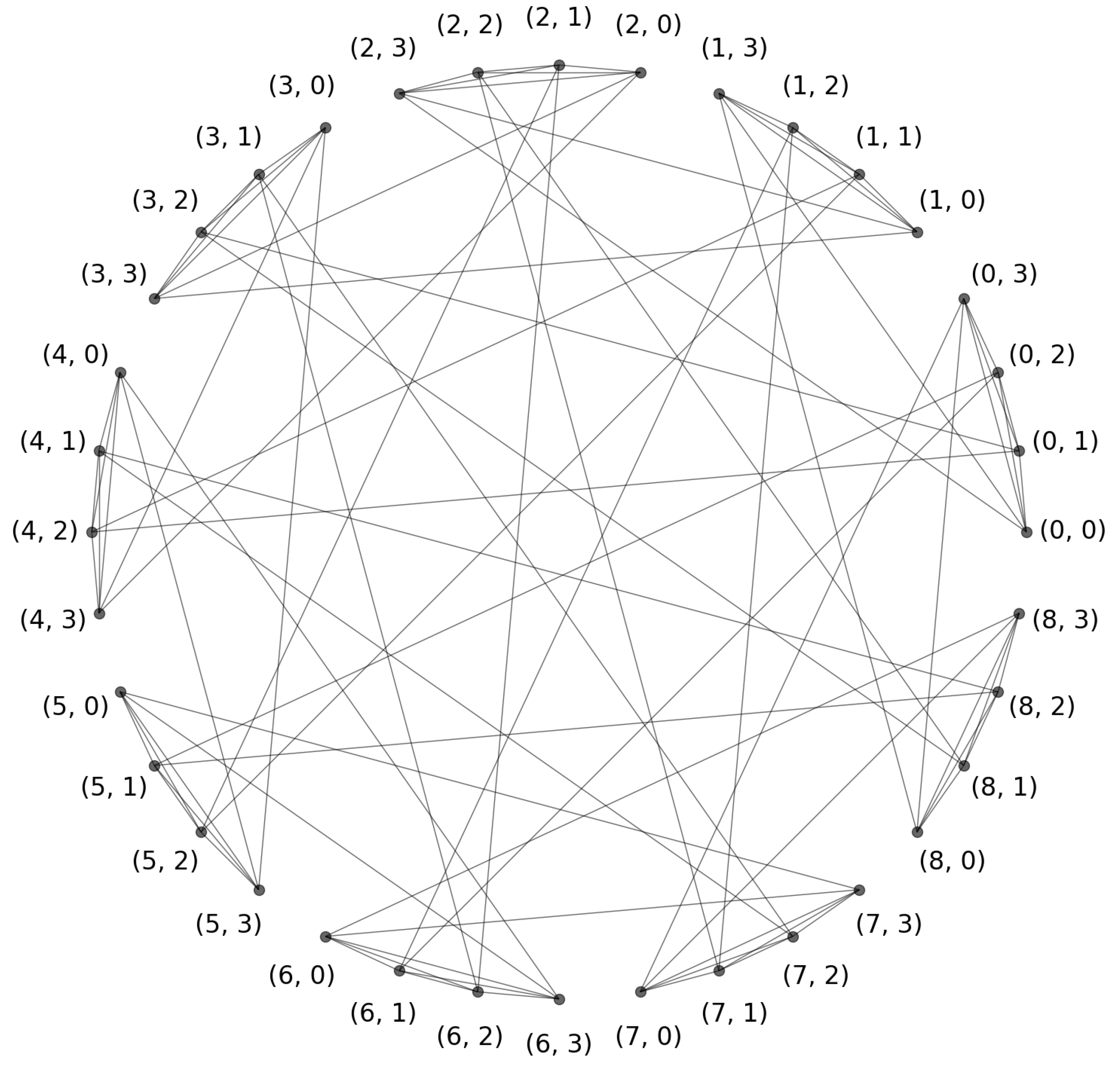
Figure 1 provides an example of
with
. This topology enables efficient data exchange and has gained attention due to its modularity, low diameter, and cost-effectiveness, making it a promising candidate for large-scale HPC applications.
Graph theory provides a foundation for studying interconnection networks, where cycle embedding properties are essential for assessing structural robustness and reliability. Given a graph
,
and
denotes all the vertices and edges in
G, respectively. The number of elements in
, written as
, is known as the
order of
G. Given a vertex
, let
denote the
neighborhood of
x in
G. A
complete graph having
n vertices, indicated by
, is such that each vertex is adjacent to every other vertex within the graph. For a cycle
C (path
P), the length of a cycle (path), denoted by
(
), refers to the number of vertices within the cycle (path). A cycle in graph
G that includes every single vertex of
G is known as a
Hamiltonian cycle. A graph that possesses a Hamiltonian cycle is called
Hamiltonian. A graph with an order of
n is regarded to be
pancyclic if it has cycles of all possible lengths ranging from 3 to
n. In particular, we term
G as
vertex-pancyclic (respectively,
edge-pancyclic) when every vertex (respectively, every edge) is included in a cycle whose length
ℓ satisfies
. In graph
G, when there is a set of
ℓ cycles
whose vertex sets are disjoint and
, we say the set covers
G and is called an
ℓ-disjoint-cycle-cover. Prior research has established fundamental properties of
, such as Hamiltonian and pancyclicity [
2].
A significant extension in graph theory is the concept of
two-disjoint-cycle-cover pancyclicity introduced by Kung and Chen [
3], which integrates the concepts of disjoint-cycle-cover and pancyclicity and ensures that a graph can be partitioned into two vertex-disjoint cycles of variable lengths. Formally, a graph
G is two-disjoint-cycle-cover
-pancyclic if for any integer
ℓ with
, there exist two vertex-disjoint cycles
and
in
G such that
and
. This property has been extensively investigated in other network topologies (e.g., crossed cubes [
3], locally twisted cubes [
4], bipartite generalized hypercube [
5], bipartite hypercube-like networks [
6], balanced hypercubes [
7], augmented cubes [
8,
9], alternating group graph [
10], data center networks [
11], bubble-sort star graphs [
12], split-star networks [
13], star graphs [
14]), as it enhances fault-tolerant routing and load balancing capabilities. However, for dragonfly networks, the two-disjoint-cycle-cover pancyclicity problem remains unexplored.
This paper fills the above theoretical gap by proving that
is two-disjoint-cycle-cover
-pancyclic, where
and
. In other words, we can find two cycles
and
in
with disjoint vertex sets, where
and
with
. Our result expands the existing knowledge in [
2] regarding the Hamiltonicity and pancyclicity of dragonfly networks. Moreover, we can obtain
is a vertex-disjoint-cycle-cover.
The rest of the paper is organized as follows.
Section 2 presents the definitions and preliminary knowledge that will be employed across the whole paper.
Section 3 and
Section 4 prove the main theorem for
and
with
, respectively. Finally,
Section 5 concludes the paper.
2. Preliminaries
The dragonfly network is defined as follows.
Definition 1. [15] Let be any positive integers that satisfy the condition . The definition of is presented in the following manner.
The vertex set of is given by , where for each i from 0 to , is a complete subgraph isomorphic to , representing the i-th group within . Moreover, and are disjoint, i.e., , where and ;
Any vertex of can be labeled by , which denotes vertex y belonging to group x, with and ;
The vertex is adjacent to vertex with if and only if , , where k ranges from 1 to r.
Obviously, is a graph with a regularity of and contains vertices. For any , we call the internal neighbor set of u. In contrast, the external neighbor set refers to the set of r vertices from other groups adjacent to u. Similarly, for any edge , we call e an internal edge if ; elsewise, e is called an external edge.
There are some results in [
2] about the Hamiltonicity and pancyclicity of dragonfly networks as follows:
Theorem 1. [2] For and , is Hamiltonian.
Theorem 2. [2] For and , is vertex-pancyclic.
By Definition 1, precisely one external edge exists between any two different groups. The endpoints of this edge are determined by the following theorem [
15]. This theorem is of great significance and serves a crucial function in the proof of our primary result.
Theorem 3. [15] The external edge connecting group i and group j is , with .
Lemma 1. [2] For , and , we have , where .
Lemma 2. For , a Hamiltonian cycle can be found in where .
Proof of Lemma 2. For , by Theorem 3, there is an external edge and . Since with , between any pair of vertices in , we can find a Hamiltonian path. Let be a Hamiltonian path between and in , be a Hamiltonian path between and in , be a Hamiltonian path between and in for any .
By Theorem 3,
with
. Thus, in
, we can find a Hamiltonian cycle:
□
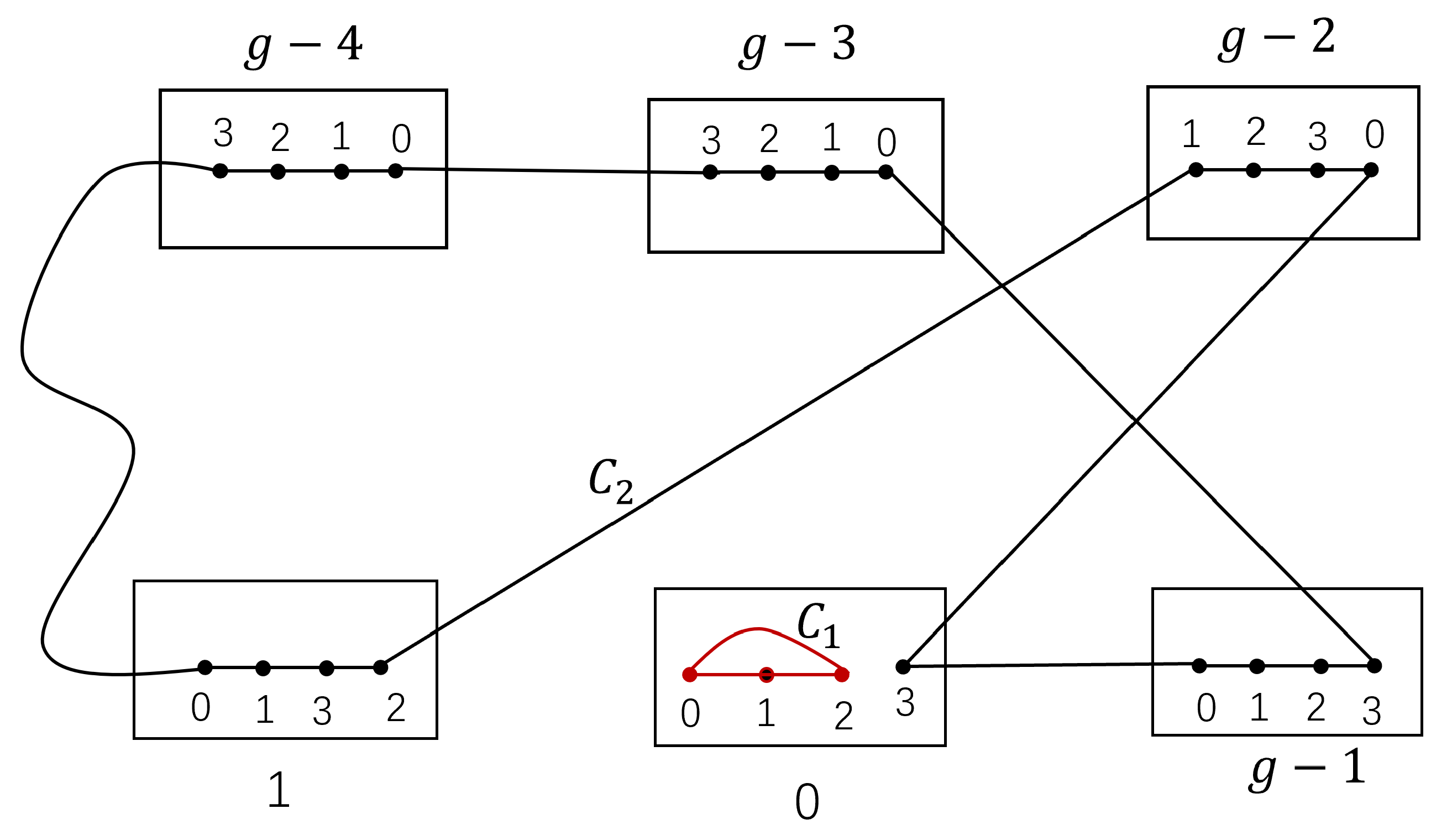
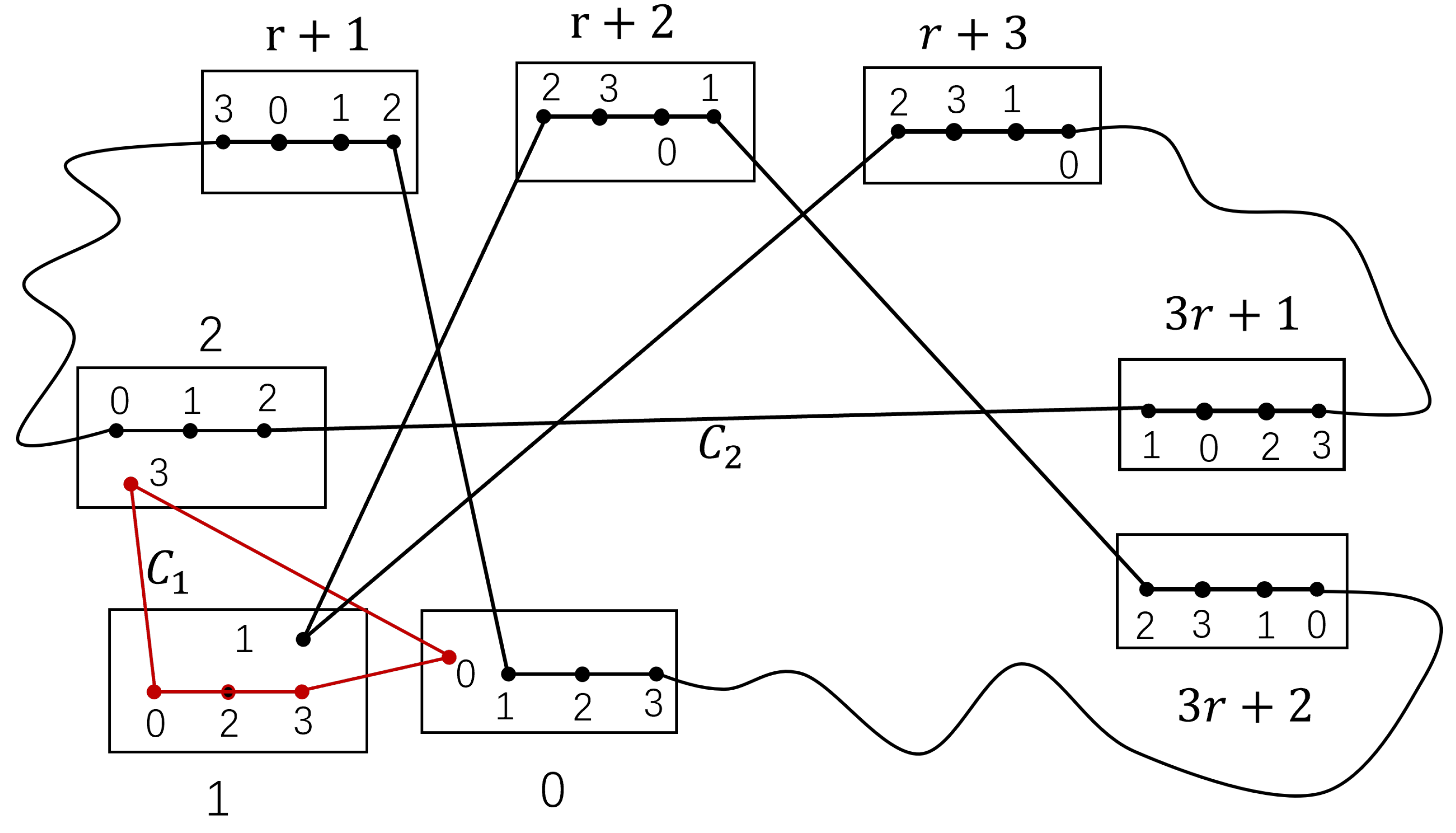
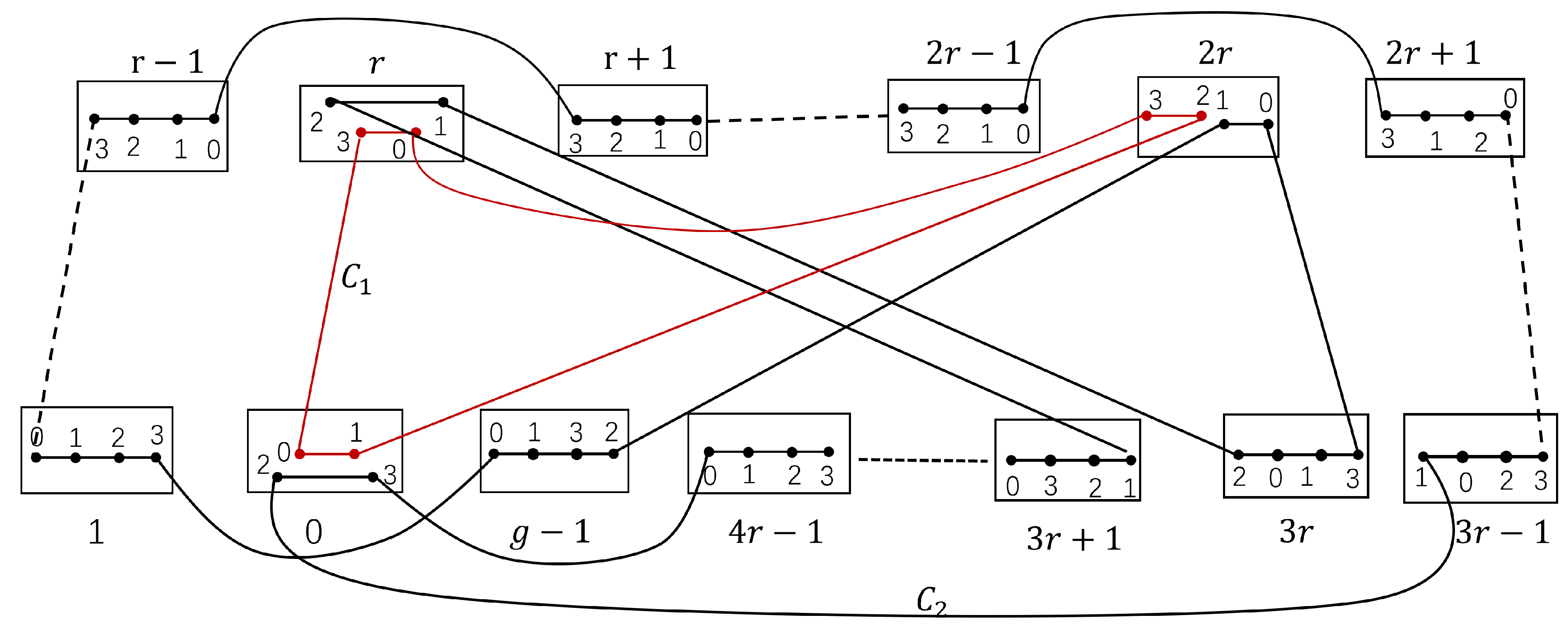
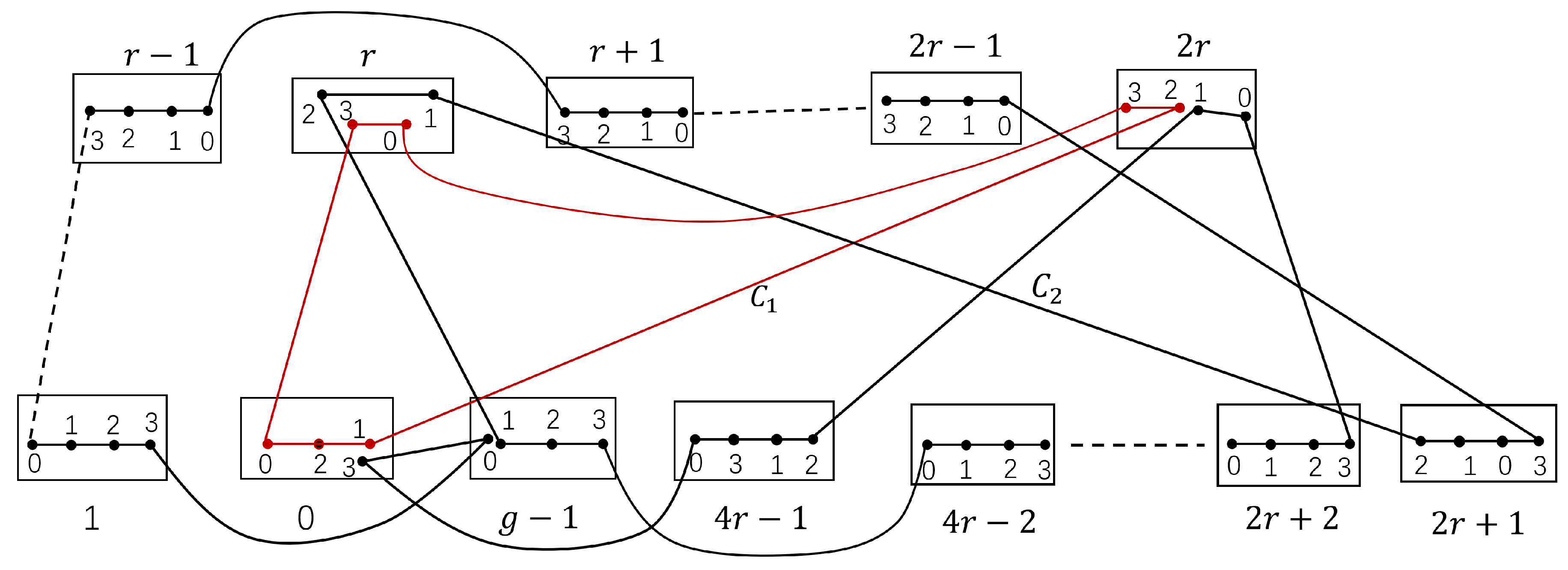
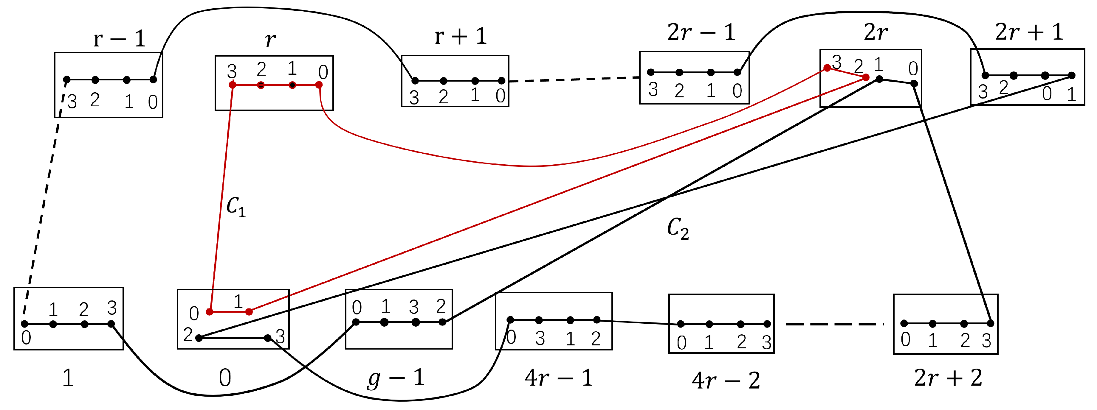
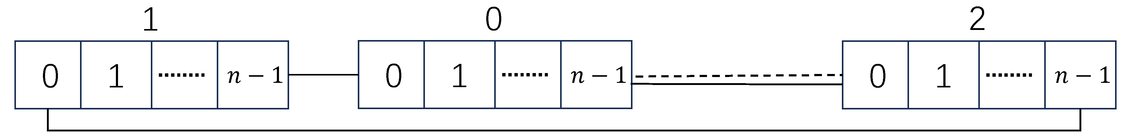
Since
is a complete graph with
, then between
and
, there is a Hamiltonian path
. By Theorem 3,
. By Theorem 1, there is a Hamiltonian cycle (see
Figure 2)
This cycle will play a crucial role in the proof of our result.
Let us consider the two-disjoint-cycle-cover pancyclicity problem of .
If , by Definition 1, is a complete graph, thus it is clear to show the two-disjoint-cycle-cover pancyclicity in .
If , there is no cycle of length 3 in .
If and , there are no cycles of length ℓ with .
If and , we obtained Theorem 4, which is the main result of this paper.
Theorem 4. is two-disjoint-cycle-cover -pancyclic, where and .
The proof of Theorem 4 is primarily structured into two parts:
Section 3 addresses the case
, while
Section 4 generalizes the result to
. For
, the proof approach is analogous to that for
, but to avoid redundancy, we computationally verify the two-disjoint-cycle-cover pancyclicity of
(with
) using a Python implementation. This code, available at
https://github.com/guanlin-he/disjoint-cycle-pancyclicity-dragonfly, leverages depth-first search and backtracking algorithms to exhaustively validate the property.
Our finding generalizes prior results in [
2] (Theorems 1 and 2) about the Hamiltonicity and pancyclicity of
. And we have the following corollary.
Corollary 1. is vertex-disjoint-cycle-cover, where and .
3. Two-Disjoint-Cycle-Cover Pancyclicity in with
This section focuses on proving the two-disjoint-cycle-cover
-pancyclicity of
with
(formally presented by Theorem 5), which serves as a foundational case for the general result in Theorem 4. The proof proceeds by case analysis, covering different ranges of
ℓ. Although the approach involves multiple cases, we strive to group similar scenarios and leverage the symmetric properties of
to reduce redundancy. Each case constructs cycles explicitly, using paths and edges derived from the graph’s topology. The detailed analysis here will provide a blueprint for extending the result to general
in
Section 4.
Theorem 5. For , is two-disjoint-cycle-cover -pancyclic.
Proof of Theorem 5. Note that, by Definition 1, with . Thus, . We only need to prove that has two cycles and where and with .
For each
ℓ within
, we found the two cycles
and
presented in
Table 1 and the corresponding figures, where
denoted a hamiltonian path between any two vertices in
for
. For a cycle
, we denote by
be a path between
and
in
C. Let
. Similarly, we denote by
and
.
Figure 3.
The cycles and with in .
Figure 3.
The cycles and with in .
Figure 4.
The cycles and with in .
Figure 4.
The cycles and with in .
Figure 5.
The cycles and with in .
Figure 5.
The cycles and with in .
Figure 6.
The cycles and with in .
Figure 6.
The cycles and with in .
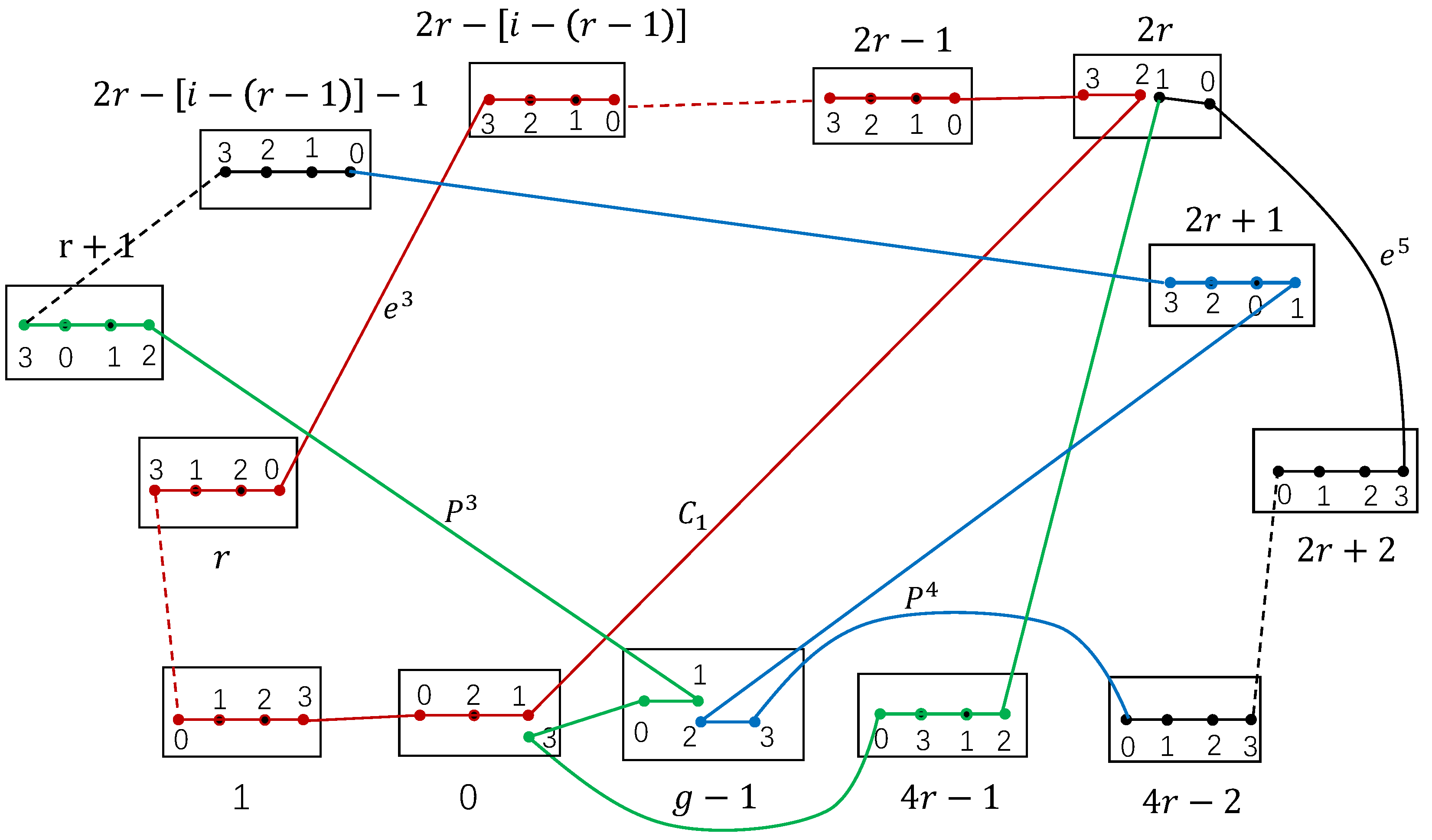
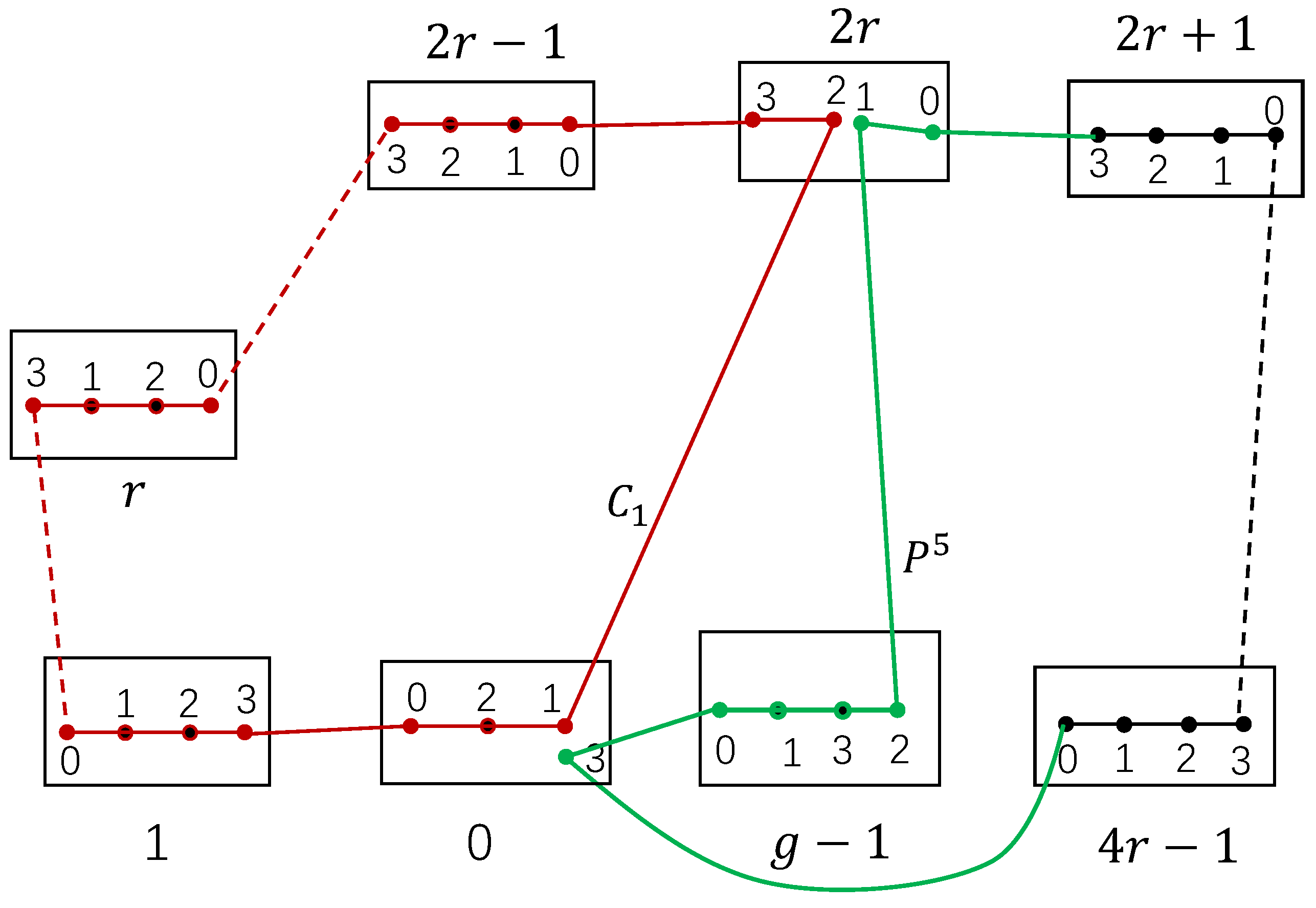
Figure 7.
The cycles and with in .
Figure 7.
The cycles and with in .
For , we present the following claims and prove their validity in turn.
Claim 1. For , two vertex-disjoint cycles , can be found in , where , .
Proof of Claim 1. It follows from in . For , since is a complete graph, there is a Hamiltonian path between and in . Let , where .
There are two paths:
with
and
with
such that
and
. By Theorem 3, let
such that
, there is a cycle of length
ℓ:
where
since
According to the range of i, we can obtain a cycle of length :
When
, let
with
and
. There are paths
and
in
such that
and
. Then
Let
. We have
and
with
. So,
When
, there are paths
with
and
with
in
. By Theorem 3, let
. Thus,
Let
. We have
,
and
. Then,
When
, there is a path
with
and
in
. Thus,
where
So,
,
are two disjoint cycles of
, where
,
(see
Figure 8,
Figure 9 and
Figure 10). □
Using the same argument as for claim 1, we can get the following claims.
Claim 2. For , two vertex-disjoint cycles , can be found in , where , .
Proof of Claim 2. Since is a complete graph, for , there is a Hamiltonian path between and in .
We have two paths: with , and with . We have and .
Let
with
. By Theorem 3, let
be such that
. There is a cycle of length
ℓ:
where
since
According to the range of i, we can obtain a cycle of length :
If
, there is a path
with
in
, by Theorem 3. Let
and
,
,
. Thus,
Let
. We have
and
. So,
If
, there are paths
and
in
with
and
. Then
Let
. We have
and
,
. So,
If
, there is a path
with
in
by Theorem 3. Thus,
Let
. We have
. Thus,
Then and are two disjoint cycles of , where , . □
Claim 3. For , two vertex-disjoint cycles , can be found in , where , .
Proof of Claim 3. It follows from in . Since is a complete graph, for , there is a Hamiltonian path between and in . Let . By Theorem 3, let be an edge such that .
There are two paths: , and .
We have
,
,
and
. There is a cycle of length
ℓ:
where
since
According to the range of i, we can obtain a cycle of length :
When
, there are paths
with
and
with
in
. By Theorem 3, let
and
be two edges. Thus,
Let
. Then
with
and
. We have
When
, there is a path
with
in
. By Theorem 3, let
. Thus,
Let
. We have
and
. So,
So, and are two disjoint cycles of , where , . □
Claim 4. For , two vertex-disjoint cycles , can be found in , where , .
Proof of Claim 4. It follows from in . Since is a complete graph, for , there is a Hamiltonian path between and in . Let with .
There are two paths: , and .
We have
and
. By Theorem 3, there is an edge
such that
. So, there is a cycle of length
ℓ:
where
since
According to the range of i, we can obtain a cycle of length :
When
, by Theorem 3, let
,
and
. Thus,
Let
. Then
. We have
When
, by Theorem 3, let
and
. We have
Thus,
where
So, and are two disjoint cycles of , where , . □
By the above case analysis, two vertex-disjoint cycles , can be found in with , , where . □
4. Two-Disjoint-Cycle-Cover Pancyclicity in with and
In this section, we focus on proving the two-disjoint-cycle-cover
-pancyclicity of
with
and
, extending the result from
Section 3 to prove Theorem 4. The proof builds on the techniques developed for
but adapts them to handle the cases of larger
n. We partition the range of
ℓ into three main cases (Case 1:
; Case 2:
; Case 3:
) to systematically address all possible cycle lengths. Each case leverages the Hamiltonian cycle
(defined in
Section 2) and the complete graph structure of the groups
. By combining path constructions, edge manipulations, and inductive arguments, we demonstrate the existence of the required cycles
and
for every
ℓ. While the proof involves case analysis, we emphasize the unifying principles, such as the use of symmetry and recursive group-based constructions, to provide insight into the general problem. This structured approach ensures rigor while minimizing ad-hoc computations.
Since
with
, so
contains a cycle of length
ℓ, where
. As
possesses the property of rotational symmetry, we can pick group 0 as a representative case without loss of generality. Let
such that
and
such that
. Now, we show
. There is a cycle of length 4:
Since with , there is a Hamiltonian path between and in and a Hamiltonian path between and in . When , there is a Hamiltonian path between and in . By Lemma 1, let be a path such that , and , , be two edges.
By Theorem 3 and Lemma 1, there is a cycle of length
:
where
So , are proved to be two disjoint cycles of , where , .
If and , by Lemma 2, then there are two disjoint cycles, one of which has a length of 5 and the other has a length of .
If
and
, there is a cycle of length 5:
When , there is a Hamiltonian path between and in .
There is a cycle of length
:
where
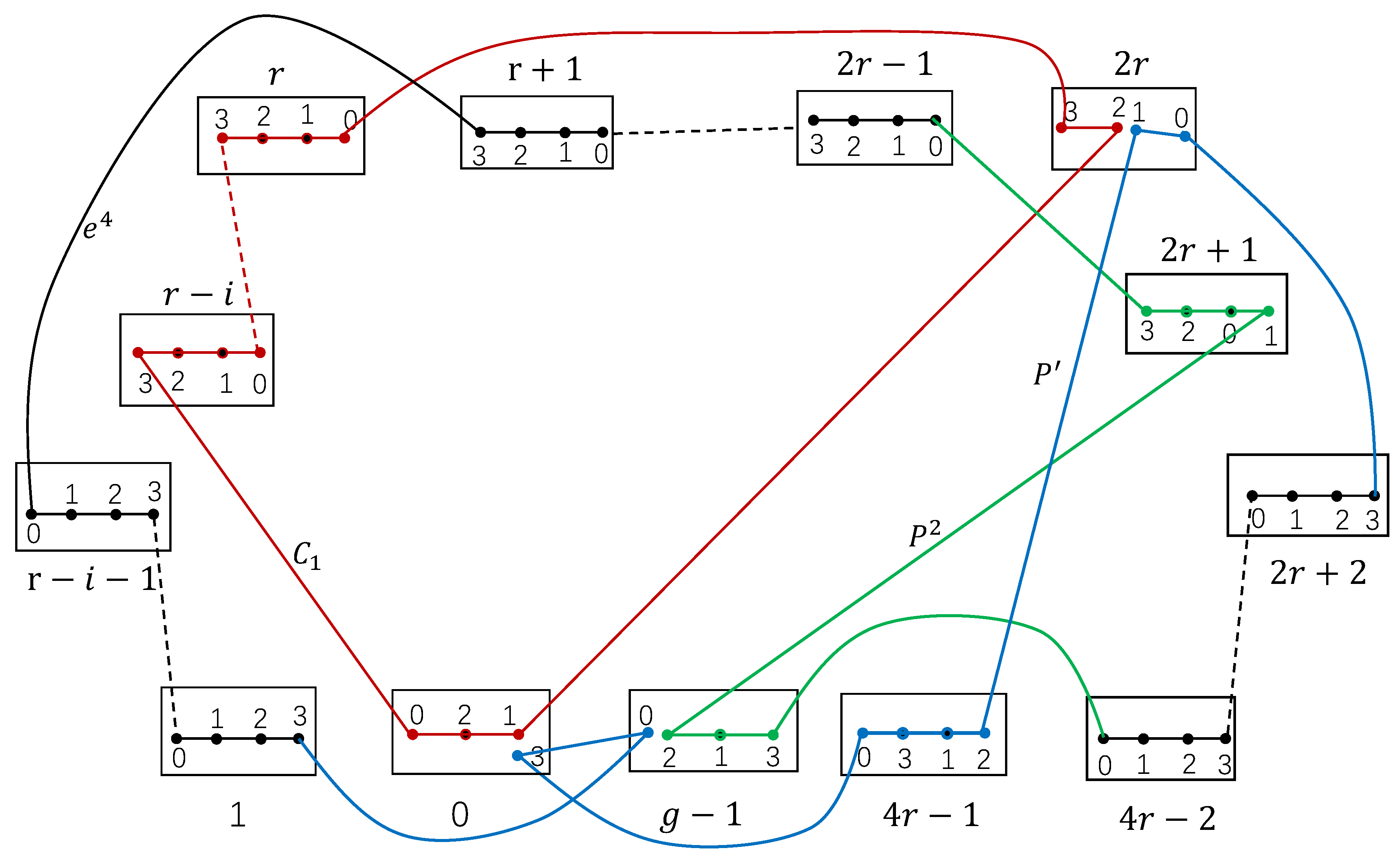
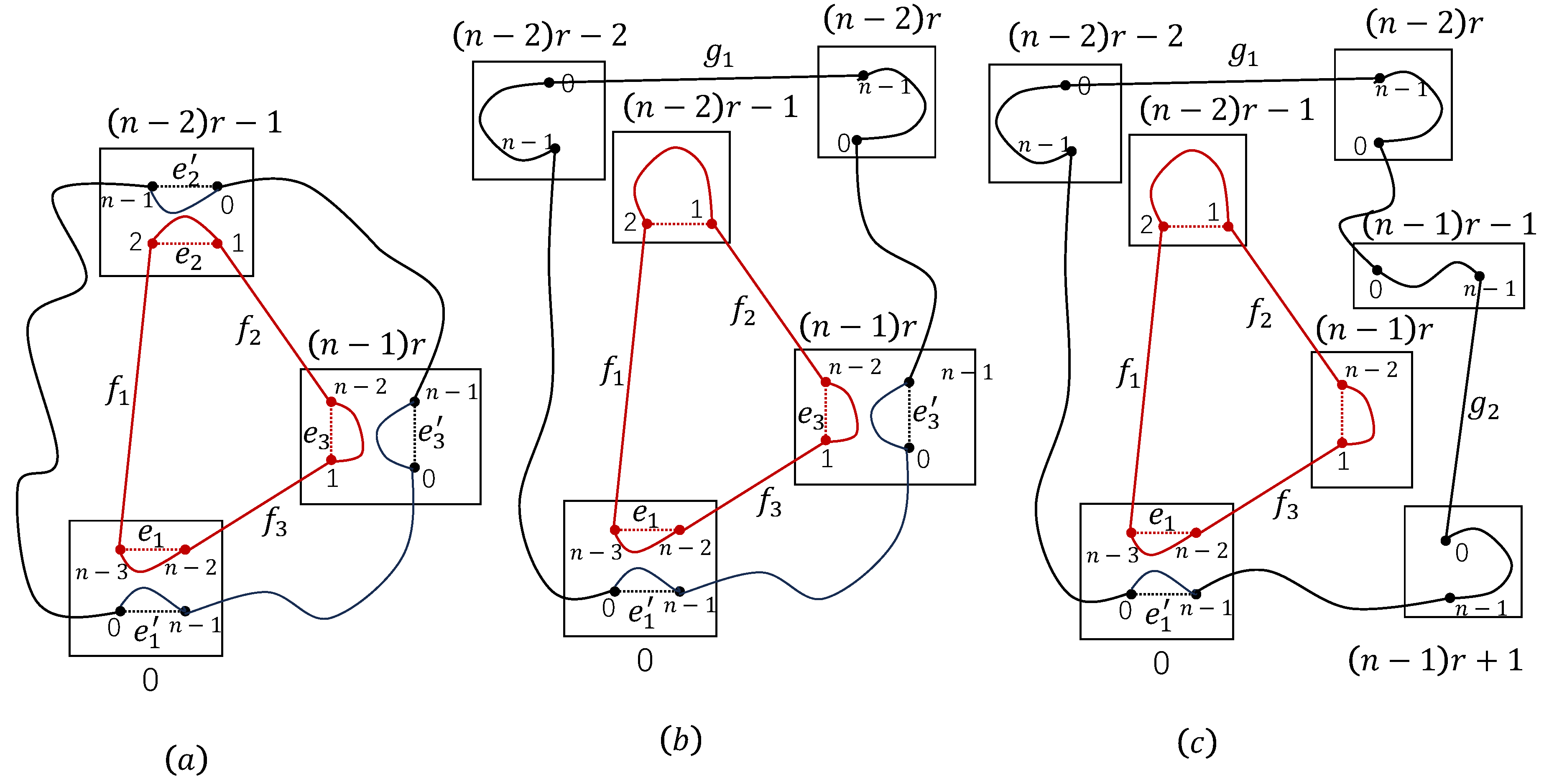
Case 2.
By Theorem 3, let , and . Then there is a cycle of length 6: in containing , and .
Since is a complete graph, there are some edges , ,, , and . Let . For convenience, let such that .
Since
, there is a path
between
and
in
with
, a path
between
and
in
with
, a path
between
and
in
with
, a path
between
and
in
with
,where
. Let
and
Then
and
(see
Figure 11) are proved to be two disjoint cycles of
, where
,
and
. Let
. Then
.
Let
between
and
in
with
, a path
between
and
in
with
,
and
. Then
and
are proved to be two disjoint cycles of
, where
,
and
, with
, see
Figure 11.
Then
and
are proved to be two disjoint cycles of
, where
,
and
, with
, see
Figure 11.
Since , then and . Thus, there exist two disjoint cycles, one of which has a length of ℓ and the other has a length of with .
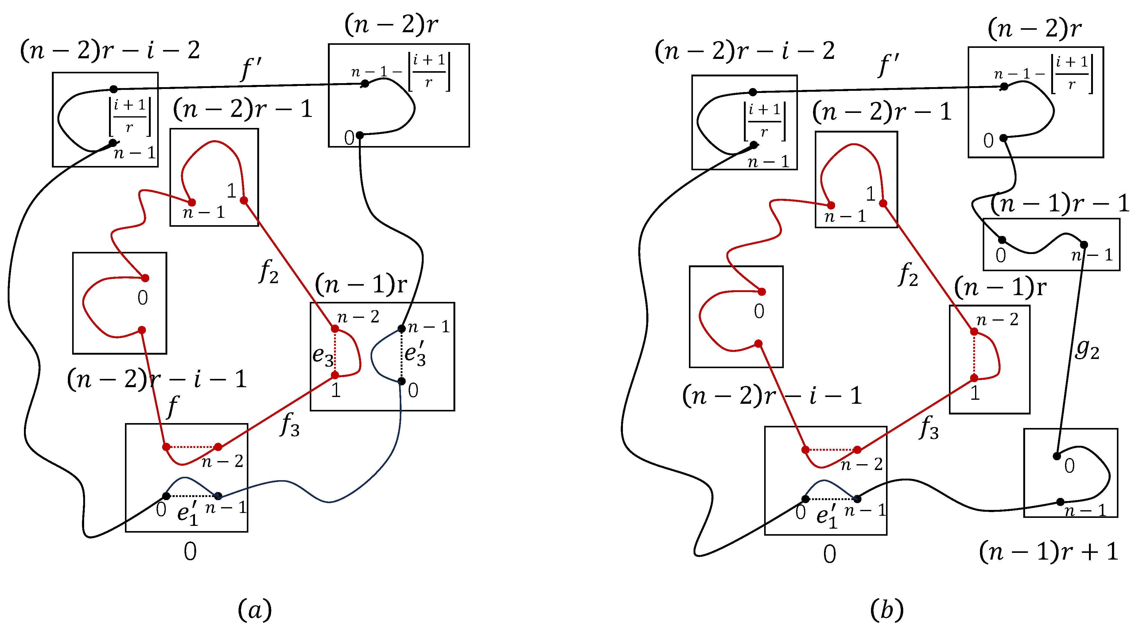
Case 3. .
We will show that has two disjoint cycles and , where , with , and .
By Theorem 3, let
and
. Since
and
, then
In order to prove case 3, we use the symbol in Case 2. Let and . Hamiltonian paths can be found between and in with . And we have a Hamiltonian path T between and in and a Hamiltonian path between and in .
Then
and
are two disjoint cycles, where
,
with
, see
Figure 12.
In addition, we have two disjoint cycles in
:
and
, where
and
with
, see
Figure 12. Since
, then
. Thus, there are two disjoint cycles
,
of
, where
,
with
and
.
Since
and
,
and
. Also,
So, .
If
, then
that is,
. So
, that is,
.
Thus, if , .
Now we show when , Case 3 holds.
Since and with , then . Now we will prove that two disjoint cycles R and can be found in , where , with .
By Theorem 3, let , , with . Let , . There exist Hamiltonian paths between and in with . And we have a Hamiltonian path W between and in and a Hamiltonian path between and in , a Hamiltonian path between and in .
Let be a path between and in , be a path between and in be a path between and in , be a path between and in , where and with .
There exist two disjoint cycles
and
Then and are two disjoint cycles of , where , with .
Then and are proved to be two disjoint cycles of , where , with .
Since
and
, so
And .
Thus, there are two disjoint cycles R and of , where , with .
Considering all the cases discussed above, two vertex-disjoint cycles and can be found in , where , with . Therefore, has two-disjoint-cycle-cover -pancyclicity for and .