
Submitted:
16 October 2025
Posted:
17 October 2025
You are already at the latest version
Abstract
This work formalizes the notions of structure and pattern for three distinct one-dimensional spin-lattice models (finite-range Ising, solid-on-solid and three-body), using information- and computation-theoretic methods. We begin by presenting a novel derivation of the Boltzmann distribution for finite one-dimensional spin configurations embedded in infinite ones. We next recast this distribution as a stochastic process, which lets us analyze each spin-lattice model with the theory of computational mechanics. In this framework, the process’ structure is quantified by excess entropy E (predictable information) and statistical complexity Cμ (stored information), and the process’ structure-generating mechanism is specified by its ϵ-machine. To assess compatibility with statistical mechanics, we compare the configurations jointly determined by the information measures and ϵ-machines to typical configurations drawn from the Boltzmann distribution, and we find agreement. We also include a self-contained primer on computational mechanics and provide code implementing the information measures and spin-model distributions.
Keywords:
Statistical mechanics
; Information theory
; Stochastic processes
; Complexity measures
; Computational mechanics
; Spin models
; Ising model
1. Introduction
When observing a natural system, we intuitively explain it by describing the way its components are arranged. We might say that the system displays order or randomness. We might describe systems that exhibit a blending of order and randomness as complex or structured1[1]. Moreover, we might also regard as structured those ordered systems that have no randomness but exhibit a repetition of more than one component (a period greater than 1) [2]. Altogether, we might regard a structured system simply as one that exhibits patterns [3].
In light of this depiction, a physicist may feel compelled to bring clarity and definiteness to the notions of randomness, structure and pattern by formalizing them. Although statistical mechanics readily concretizes randomness through measures like entropy [4,5], it falls short when quantifying structure and pattern and formalizing its supporting mechanism. For instance, while magnetization is commonly treated as an indicator of structure, materials with distinct magnetic behaviors, such as paramagnets and antiferromagnets, have the same magnetization in the absence of a magnetic field: zero [2]. Faced with these limitations, the physicist may make their endeavor more concrete by posing two key questions:
- (1)
- What’s a simple system in statistical mechanics that manifests structure and patterns?
- (2)
- How could one extend statistical mechanics to formalize structure and patterns within such a system?
One-dimensional (1D) spin lattice models [6] (p. 67) are suitable candidates for addressing these challenges, as they compactly represent interacting magnets as spins in an evenly spaced grid, embodying both simplicity [7] and structure/patterns [8]. The simplicity stems from the spins taking discrete values (often binary) and the spin models being amenable to both analytical and numerical treatment [9,10]. The structure and patterns are evident in the model’s possible spin configurations, which exhibit regularity, randomness and structure. For example, the 1D nearest-neighbor Ising model may have configurations rich in regularity, randomness and structure such as: , and , respectively. These configurations contain repeating sequences of spins that we refer to as configuration patterns.
Mathematically, a spin model is expressed as a Hamiltonian that characterizes the energy of the spin system [6] (p. 67). Given the Hamiltonian, the usual goal is to determine the partition function and from it compute various properties of interest [11]. Among these, the Boltzmann distribution as a function of spin configurations is the least frequently computed2, yet it stands out as the sole one directly addressing spin configurations, serving as a window for analyzing their structure and patterns. However, to clearly see through this window, we need to carefully consider how the distribution is formalized.
Typically, the Boltzmann distribution is defined so that each configuration, either implicitly or explicitly, represents an event of a single random variable, as indicated in Refs. [17] (p. 552) and [18]. Nonetheless, this approach is not conducive to examining how individual spins make up spin configurations. Instead, we can regard them as realizations of a partially ordered chain of random variables—a stochastic process [2].
In this process, which we call the spin process, each spin corresponds to an event of a single random variable. Given this perspective, we can now quantify the randomness, regularity, and structure of the spin process, and formalize the mechanism that generates its structure. Since randomness, regularity, and structure are ways in which a process elicits surprise, we quantify them as information—a measure of “quantifiable surprise" [19] (p. 64) or a “difference that makes a difference” [20].
In information theory, the theory of quantifiable surprise, a stochastic process’ intrinsic randomness or average randomness per symbol is quantified by its Shannon entropy rate (Ref. [21], pp. 74-76). The process’s regularity, as the counterpart of its randomness, can be understood as the total correlation within the process. Thus, regularity is quantified as the amount of information that is shared within the process—that is, the process’ mutual information or excess entropy E [22,23,24,25].
Because a stochastic process’s structure is effectively captured by its patterns, we quantify the process’s structure by measuring the amount of information stored in those patterns. This quantity is known as the stored information, or statistical complexity [26,27], and is defined as the Shannon entropy of those patterns. Calculating therefore requires identifying these patterns—an inference task that effectively uncovers the process’s underlying structure-generating mechanism. We define these patterns next.
Since patterns are sought for their predictive utility, we define a pattern in the spin process setup from a prediction-based viewpoint. To do so, we split3 each realization of the spin process into a left half (past) and a right half (future). Then, we define a pattern as the set of pasts that lead to the same futures4 [28]. By “lead to” we mean that the conditional distribution over futures, when conditioned on any past in the set, is identical across all those pasts. This condition is known as the causal equivalence principle5 [27,28,29], which recasts these patterns as causal states. Why the term “state"? Because this conception of pattern is consistent with theory of computation’s definition of state as a system’s entity that “remembers a relevant portion of the system’s history" [30] (pp. 2-3). This connection points us toward the mechanism that underpins the process’s structure.
Given that a system’s structure is measured in units of information, formalizing its supporting mechanism is tantamount to unraveling how the system processes and stores information—essentially, how it computes [31]. This leads to a refined question: what is the minimal6 abstract machine7 that performs the computation inherent to the spin process? Leveraging concepts from TOC, computational mechanics provides a compelling response: the set of causal states and their transitions, that is a -machine or Probabilistic Deterministic Finite State Machine (PDFM). Here, “probabilistic" means that state transitions include probabilities, while “deterministic" implies that when we have knowledge of a state and its associated outgoing symbol, we have complete certainty about the next state we will transition to. Several methods have been developed for inferring -machines [32,33,34,35,36,37,38]. Among these, Feldman and Crutchfield’s approach stands out as the only one that is both analytical and applicable to statistical mechanics [2].
In particular, Feldman and Crutchfield used this method to examine the structure of the nearest-neighbor and next-nearest neighbor Ising models. Subsequent research further developed their information-theoretic analysis of spin systems by calculating and for the two-dimensional nearest neighbor Ising model [39], as well as decomposing the nn Ising model’s Shannon entropy rate into more refined information components [40]. Moreover, quantum -machine formulations revealed striking memory advantages—ranging from extreme compression when simulating long-range Ising spin chains [41] to clarifying how simplicity differs in quantum versus classical descriptions [42]. Now, the aim of this paper is to develop information measures and -machines for three varied one-dimensional spin-lattice models—finite-range Ising, solid-on-solid, and three-body—and to assess the consistency of these results with statistical mechanics.
These developments are timely because they broaden the rapidly evolving landscape of abstract machines used to analyze computation in physical processes in two key ways. First, they encourage the application of abstract machines—which have most often been used to study thermodynamic [43,44,45,46] and quantum [47,48,49,50] processes—to statistical mechanical processes, potentially supporting more efficient information processing in materials. Second, these developments foster the use of abstract machines that are systematically inferred from data, rather than being designed in an ad hoc manner, as has more typically been the case.
To achieve the aim of this paper, we provide a pedagogical explanation of computational mechanics’ application to the nn and nnn Ising models, along with the necessary background from statistical mechanics, measure theory, stochastic processes, and information theory. We then apply these techniques to a wider range of spin models such as finite range Ising models, solid-on-solid models, and three-body models. In parallel, we find that the typical patterns observed in these spin models at various parameter values match those predicted by information measures and -machines. This allows us to present an account of spin patterns clearly consistent with statistical mechanics and information/computation theory.
2. Background
2.1. Spin Measurements: Boltzmann Distribution of Finite Chain Embedded in Infinite Chain
The Boltzmann distribution serves as an entry point for probing the structure of spin models; however, defining it for both finite and infinite configurations introduces significant difficulties. For finite configurations, the Boltzmann distribution lacks generality and often relies on numerical simulations for approximation [51,52,53]. For infinite configurations, a different issue arises: their probability is zero [54] (pp. 94-97). This defies our expectation of them occurring and results in an unnormalized total probability—a sum that is zero instead of one. To balance the constructiveness of finite configurations with the generality of infinite ones, we examine a hybrid configuration: a finite spin configuration embedded in an infinite one [55]. Figure 1 illustrates the finite configuration embedded within the infinite one. The key equations leading to the embedded distribution are presented below, with detailed derivations provided in Appendix F, Appendix G, Appendix H and Appendix I.
Consider a configuration consisting of N spins, where each spin can take one of two values (↑ or ↓) and interacts only with its nearest neighbors. For convenience, the configuration is subject to periodic boundary conditions:
The system is governed by a translationally-invariant Hamiltonian, that is, a Hamiltonian whose form remains the same across spin sites. It is defined as:
Next, the corresponding transfer matrix, with components , is expressed as [6] (p. 68):
Then, the probability distribution for this spin configuration in the thermodynamic limit is obtained in terms of the transfer matrix components and the transfer matrix’s principal eigenvalue [6] (pp. 68-69):
Now, consider a specific finite configuration of length L embedded in an infinite one
Although the principal eigenvectors of the transfer matrix are seldom calculated in studies of spin models, they play a crucial role in defining the embedded distribution. Therefore, we obtain the normalized principal left and right eigenvectors of the transfer matrix, as provided in Ref. [6] (pp. 72-73). For conciseness, these are expressed in terms of the magnetization m, as shown below:
Notice that for the nn Ising model, the left and right eigenvectors are identical. Hence, in all subsequent subsections of this section, we omit the left and right superscripts.
Lastly, the probability distribution for the embedded configuration [55] is given by
Here, we provide the physical interpretation for each part of the equation:
- In the denominator, is raised to as each embedded configuration has L spins and its boundaries are not periodic.
- In the numerator, the product of transfer matrix components consists of factors. This reflects the fact that only the spins within the bulk have neighboring spins to interact with on both their left and right sides.
- Also in the numerator, we include two extra terms: and , which are the normalized principal eigenvector components associated with the boundary spins and . Since the embedded configuration does not have periodic boundaries, these extra terms ensure that the boundary spins contribute to the system’s magnetization as much as the bulk spins. Moreover, these terms are key for normalizing the joint probabilities.
To facilitate later discussion, it will be useful to denote the component associated with spins ↑ or ↓ as , and , respectively. The values of these components correspond to either or , depending on whether the orientations of the spins and are up or down. For example, in a spin configuration like , the component for the first spin is , while the component for the last spin is .
Alternatively, equation (7) can be interpreted as the probability measure of a coarse-grained configuration. The nature of this coarse-graining and its implementation, which relies on measure theory, will be discussed in the following section.
2.2. Coarse-Graining via Measure Theory
In this section, we view finite configurations embedded within infinite ones as coarse-grained versions of infinite spin configurations. Here, “coarse-grained" means a simplified representation that retains essential features while reducing detail [56]. The procedure for arriving at these representations—that is, coarse-graining—is up to the scientist’s discretion [57]. However, when treating the spin model as a stochastic process, the conventional approach is to reduce the degrees of freedom such that only contiguous ones remain [58,59,60]. This coarse-graining is physically motivated by the observer’s inability to record infinite measurements or degrees of freedom. To define the set of coarse-grained configurations mathematically, we begin with the full set of possible configurations.
Consider the set of all possible infinite spin configurations . An individual configuration in this set is represented as . The degree of freedom at lattice site i within a configuration is denoted by . Thus, a configuration in terms of its degrees of freedom is given by
with
The set of coarse-grained configurations is defined as the set of infinite configurations in which the contiguous spins from to have fixed indices and can take any value from .
This can be expressed as
Alternatively, the set of coarse-grained configurations can be defined as
with each coarse-grained configuration defined as
where represent the fixed spin values at fixed indices . In more compact notation, this is written as:
Notably, the act of coarse-graining changes our focus from individual configurations to sets, where each set groups configurations by their shared spin values. Figure 2, shows how the set of all possible infinite spin configurations is partitioned into the set of coarse-grained configurations . Accordingly, we must adapt our notion of probability to match this perspective, transitioning from the concept of a probability distribution to that of a probability measure, denoted by [61] (pp. 331-336).
To formalize this, we introduce the concept of a sigma algebra, denoted by . This is a collection of all subsets of that can be consistently assigned probabilities or measured, meaning they are physically relevant.
The sigma algebra has three key properties:
- Entire Set Containment: includes the sample space. In this case, that is the coarse-grained set of all infinite configurations :
- Complement Closure: If a set A is in , then its complement must also be in :
- Countable Union Closure: If are in , then their countable union is also in :
With the concept of a sigma algebra established, we can now turn to the probability measure. This measure is analogous to a probability distribution, but applies to sets rather than individual outcomes. It extends the key constructive properties of probability distributions—namely, nonnegativity, normalization and additivity—from finite to infinite configurations.
The probability measure is formalized as a function
that assigns a probability to each event in and satisfies the following three key properties:
- Nonnegativity: In the same way that joint probabilities for finite configurations are never negative, the probability measure assigned to any set in must also be nonnegative.
- Normalization: Similar to the sum of joint probabilities for all configurations equaling 1, the probability measure for the entire sample space, the set of coarse-grained configurations , must be 1.
- Countable addivity: Mirroring the additivity of joint probabilities, which asserts that the total probability of finite configurations equals the sum of their individual probabilities, probability measures demonstrate countable additivity. This property dictates that for any countable collection of non-overlapping sets (cylinder sets) , the probability of their union is the sum of the probabilities of the individual sets:where each is a cylinder set corresponding to a coarse-grained configuration, and the union represents the combined event of these configurations.
The last step in constructing the spin probability measure involves assigning each spin cylinder set’s probability measure the value of its associated embedded configuration’s probability. Notably, information measures in later sections are denoted with a subscript, indicating that their argument is a probability measure [2].
2.3. System and Measurements: Stochastic Processes
As mentioned in the introduction, we interpret configurations as realizations of a stochastic process. This section aims to delve further into this formalism by first explaining the reasons for departing from the conventional approach.
Traditionally, a spin configuration is represented as an event s of a random variable S. For example, a configuration with all spins pointing up is depicted as:
However, this formalism impedes a direct examination of individual spins and their interactions. Furthermore, it leads to an unwieldy number of possible events. To address these issues, we adopt a more nuanced approach. Instead of representing a configuration as a single event, we depict it as a specific realization of events:
This realization is an instance of a stochastic process, i.e., a partially-ordered chain of random variables:
whose associated probability distribution is given by
Within this framework, the all-ups spin configuration is now denoted as:
Without loss of generality, we can split a process into two parts: the past process, defined as
along with its associated past realization, and the future process, defined as
along with its associated future realization.
For simplicity, we will use the terms “past" and “future" to refer to both processes and their associated realizations, with the specific meaning inferred from the context.
The spin stochastic process will be our object of study. In the following subsection, we will elaborate on how it relates to broader categories of processes, as seen in Ref. [62].
2.3.1. Types of Processes
Stationary process
A process in which the statistical properties of its random variables remain invariant over time. These properties include but are not limited to mean, variance, or joint distribution.
Strictly stationary process
A process whose joint distribution remains invariant under shifts in time. In other words, a process whose random variables are time-translation invariant. That is, a process that satisfies:
Markovian process
A process in which the probability distribution of the next random variable depends only on the preceding one. That is, a process whose joint distribution factors as follows:
R-order Markovian process
A process in which the probability distribution of the next random variable depends only on the R preceding ones. That is, a process whose joint distribution is given as follows:
Spin process
A process whose associated probability distribution is generated by a spin Hamiltonian model. For the models considered in this work (finite-range Ising, Solid on solid and Three body models), this process is strictly stationary and Markovian or R-order Markovian.
We can now define information measures of randomness, regularity and structure for a stochastic process, starting from the basics of information theory.
2.4. Information Measures
What is information? Information can be conceived as quantifiable surprise, defined in terms of probabilities [19] (p. 64). Through this lens, an event s that is not likely to occur is deemed surprising, thus carrying high informational content. This means that the information of an event is inversely proportional to its probability, that is, . More specifically, the event’s information content—termed self-information—[19] (p. 64) is defined as
Here, the presence of the logarithm is a convenient guarantee that the self-information possesses the additive property [63]. That is, the total surprise from combining events 1 and 2 equals the sum of their individual surprises.
The natural next step is to consider a random variable S. Its information content is known as Shannon entropy. It is defined as the weighted sum of the self-information of each possible event within the variable. Mathematically, it is expressed as
Following this line of reasoning, we can define the conditional entropy (Refs. [63]; [21], p. 17) as the amount of information needed to specify a random variable given that a random variable is known.
Moreover, we can define the joint entropy (Ref. [63]; Ref. [21], pp. 16-17) as the amount of information contained in two random variables.
Now, how may we define the entropy of our object of interest, that is, the stochastic process? The simplest answer would be to consider the growth entropy [64], that is, the Shannon entropy of the entire process.
However, as the length of the process increases, the growth entropy also rises and ultimately diverges when the process extends towards infinity (). This raises the question: how can we capture the total information of a stochastic process? A solution lies in the Shannon entropy rate (Ref. [64]; Ref. [21], pp. 74-76) defined as
Again, the symbol signifies that the Shannon entropy rate is calculated in terms of a probability measure. Notably, this rate can be simplified for processes that are both stationary and Markovian, like the spin process. For a stationary process, the entropy rate reduces to
If the process is also Markovian, it becomes
By recasting the Shannon entropy rate as a conditional entropy, we can understand it as the amount of surprise each spin contributes. This effectively measures the process’s randomness per spin. Furthermore, for one-dimensional spin models, the Shannon entropy rate matches the Boltzmann entropy density, the more familiar form of entropy in statistical mechanics, as shown in Appendix C.
Since the regularity of the spin process is interpreted as the information shared between the process’ past and future, the regularity is defined as the process’ mutual information or excess entropy [22,23,24,25]. Mathematically, it is defined for the spin process as follows:
Therefore,
Notably, the excess entropy can be interpreted as predictable information. That is, it quantifies the amount of information an observer has for recognizing configuration patterns, even if that information is not enough to identify them. However, in the absence of entropy rate , is sufficient to determine how much information is required for the observer to achieve synchronization with the underlying configuration patterns. Synchronization, from this purely information-theoretic perspective, refers to the observer’s ability to recognize and discern these configuration patterns.
To measure the process’ structure or statistical complexity, we need to determine the asymptotic probabilities of its patterns or causal states . In general, this often requires inferring the process’s -machine, especially for non-Markovian processes [65] (p. 37). However, for the spin process, we can calculate them directly since we have a natural definition of causal states.
Given the Markovian nature of the spin process, the next spin only depends on the previous one. Thus, the probability distribution of future spins conditioned on past ones, matches the probability distribution of the future conditioned on the previous spin being up or down. Now, since the probability of a spin up and the probability of a spin down add up to 1, and they represent the probability per site throughout the process, they can be interpreted as the asymptotic probabilities of the causal states. Therefore, the statistical complexity of the spin process can be quantified as [2]
Therefore,
These information measures can be simply related via the identity as
This relationship [65] (p. 37) formalizes our intuition that structure is a blending of randomness and regularity. Here, R denotes the neighborhood radius, which equals 1 for the nn Ising model.
Since the causal states are sufficient to predict the process’s future, and considering that prediction is tantamount to reproduction, statistical complexity can be defined as the minimum amount of information required to reproduce the stochastic process [2]. As mentioned in the introduction, if structure is viewed as quantifiable information, then this suggests that the mechanism generating the structure can be described as a machine [28,31].
2.5. Structure: Computational Mechanics
To formalize the mechanism generating a physical process’ structure, the concept of machine must be adapted to satisfy three statistical mechanical constraints:
- Be capable of reproducing ensembles
- Possess a well-defined notion of “state"
- Be derivable from first principles
Computational mechanics meets the first requirement by enhancing the simplest machine in TOC, the Deterministic Finite State Machine (DFSM), with probabilistic features while keeping its determinism intact [29,66]. The former is achieved by incorporating probabilities into the state transitions, and the latter is maintained by ensuring that the probability of transitioning to the next state, given the current state and a specific outgoing symbol, is precisely one. These modifications result in a machine known as Probabilistic Finite State Machine (PDFM) or -machine.
The second requirement is fulfilled by operationalizing TOC’s conceptual definition of a state—an entity that “remembers a relevant portion of the system’s history" [30] (pp. 2-3)—as a causal state. A causal state is the collection of all past realizations that when individually conditioning the process’ future yield the same conditional probability distribution [28,29]. Notably, formalizing the notion of “state" is crucial not just for conceptual clarity, but also to satisfy the third requirement. The reason for this is that without a clear understanding of what states are, the procedure for inferring them is much less clear.
To satisfy the third condition, we recast the definition of causal state as a guiding principle for inferring causal states from realizations, that is, the causal equivalence principle [28,29]. It dictates that two past realizations belong to the same causal state if they lead to the same conditional distributions over process’ futures. In practice, this principle allows us to construct the underlying -machine of an ensemble.
In summary, the key ingredients of computational mechanics are the concepts of -machine, causal transition, causal state, and the causal equivalence principle [29]. While we introduced them in this order to capture how they would be re-discovered conceptually, we will now present them in reverse order to delve into their mathematical details more pedagogically.
Causal equivalence principle. Two pasts are considered causally equivalent if and only if they make the same prediction over the future, i.e.
Effectively, this principle groups pasts that lead to the same future into what are known as causal states. To formalize what we mean by “leads," a causal state is defined as
Causal state. A triple that contains
- An event with its associated probability of the causal state random variable :
- A distribution of the future conditioned on the causal event, i.e., a morph:
- The set of histories that lead to the same morph:
Now, assuming that our machine is deterministic in the computation theoretic sense, we can define the causal transition as
Causal transition. The probability of transitioning from state to state while emitting the symbol
These definitions allows us to construct the minimal machine supporting a stochastic process’ structure.
-machine or PDFM. A pair that contains
- The set of causal states
- Transition dynamic (causal transitions gathered in a matrix) [27]
For inferring -machines, it will be important to distinguish between two types of causal states:
- Recurrent causal states: These are states to which the machine will repeatedly transition as it operates. Consequently, their asymptotic probability is non-zero.
- Transient causal states: These are states that the machine may reach temporarily but will not return to. As a result, their asymptotic probability is zero: .
Notably, the connectivity and number of transient states specify how difficult it is to identify the periodicity of configurations. In other words, these transient states reflect the computational effort required to achieve synchronization with the recurrent causal states. Here, synchronization is recast as the observer achieving certainty about the recurrent causal state it occupies, even in systems with nonzero entropy rate . Thus, transient states offer a computational perspective on synchronization, which completes the informational interpretation provided by the excess entropy .
Since this is a principled approach, we can infer our machine of interest, rather than design it. For spin processes, an analytical method exists for inferring recurrent causal states [2]. Moreover, transient states can be reconstructed from these recurrent states, as detailed in Appendix B of Ref. [2]. Below, we provide a step-by-step explanation of the analytical reconstruction method for recurrent causal states.
2.5.1. Analytical Method to Infer -Machines
- Consider a finite configuration of length embedded in an infinite one.
- Consider the joint probability of the embedded finite configuration.
- Compute the conditional probability of the right half of the configuration given the left half.
- Notice that the only past element the conditional probability depends on is its last spin . Thus, the conditional probability is Markovian.
- Identify morphs.
-
Identify the number of causal states.Since there are two morphs, there are twocausal states at most
- Identify sets of histories that lead to the same morph.
- Apply definition of causal transitions.
-
Calculate asymptotic causal state probabilities using two facts:Since , by inspection, we have
- Build transition dynamic T.
-
Find left eigenvector using .
- Build HMM representation of -machine using the transition matrix . Details of the resulting machine, for the parameter values , , and , are provided in Appendix E.
2.6. Patterns as -Machines
The following example illustrates how computational mechanics formalizes the concept of a pattern. Consider a spin configuration such as . When asked, “What’s the pattern in this configuration?", an intuitive answer might be . However, if presented with an ensemble of spin configurations and posed with the same question, the concept of a pattern becomes vague. To reason towards a definition of pattern for ensembles, we can ask: “What’s the key property of a pattern?" A plausible candidate is that a pattern represents a compressed form of data that enables an observer to reproduce the original content [69]. Thus, we can then ask: “What’s the object that statistically reproduces such a configuration?" The framework of computational mechanics provides the answer: the -machine, which can be interpreted as a physical or ensemble pattern [28,29]. Figure 3 illustrates the relationship between configuration and ensemble patterns.
From this point forward, the plotted machines will be derived using the CMPy package, which implements a tree-reconstruction method for inferring -machines, as described in Refs. [26,27]. The transient and recurrent states of these machines are represented in purple and green, respectively. For clarity in visualization, spins ↑ and ↓, emitted during transitions between causal states, are represented as 1 and 0, respectively. The ensembles of spin models discussed in the following section include configurations of either 4 or 6 spins. Configurations with probabilities below are excluded from consideration.
Based on Figure 3, one might be tempted to conclude that an -machine is simply a Hidden Markov Model (HMM). However, that is not the case. The difference stems from how states in HMM and -machines are characterized; specifically, a causal state in an -machine is defined as a triple, as mentioned earlier. In contrast, the conventional use of HMMs typically equates a state directly with the outcome of a random variable, treating the state as a singular entity rather than a triple. The definition of a state in computational mechanics is crucial, as it provides the foundation for inferring states from first principles rather than manually designing them [26].
3. Spin Models
As discussed in the previous section, the embedded Boltzmann distribution generates a vast number of spin configurations, making the structure and pattern of an arbitrary configuration unrepresentative of the system’s overall structure and patterns. However, to compare the information measures and -machines to the Boltzmann ensemble, it may still be useful to examine the structure and patterns of the individual configurations that are most optimally representative. To achieve this, we focus on a specific kind of configuration: typical configurations. These configurations are the most likely outcomes generated by the embedded Boltzmann distribution of a given spin model. Among these, likely typical configurations have probabilities that are significantly higher than those of non-typical configurations, whereas unlikely typical configurations have probabilities that are only slightly higher than those of non-typical configurations. The patterns present in these typical configurations are referred to as typical configuration patterns.
The patterns and structures of both typical and non-typical configurations across different spin models are shaped by various parameters [70]. To identify commonalities in how these parameters contribute to the configurations’ structure and patterns, we propose classifying them into three distinct types. To illustrate this, we will reference the nearest-neighbor (nn) Ising model as an example while defining each type of parameter.
- Randomness Parameter: This parameter governs the degree of randomness within the system. As it increases, it leads configurations to become more uniformly likely. In the nn Ising model, temperature T usually fulfills this role.
- Periodicity Parameter (Type 1): This parameter enhances periodicity and, as it varies, biases the system toward configurations that consist exclusively of a single period. In the nn Ising model, the coupling constant B exemplifies this. It induces period 1 configurations whether B is significantly positive or negative. Specifically, a high positive B biases all spins to point upwards, while a high negative B results in all spins pointing downwards.
- Periodicity Parameter (Type 2): Similarly, this parameter enhances periodicity but, as it varies, steers the system towards typical configurations with multiple distinct periods. In the nn Ising model, this role is played by the coupling constant J. A high positive J value tends to produce period 1 configurations (all spins up), akin to B, but a negative J value leads to alternating spin configurations (e.g., up-down-up-down), indicating that the typical configuration can be of period 2.
3.1. Finite-Range Ising Model
The nearest-neighbor Ising model can be generalized to a finite-range model using Dobson’s spin block method [71]. This approach consists of redefining the model’s degrees of freedom from individual spins to blocks of spins. These spin blocks are only allowed to interact with their nearest neighbor blocks. Equivalently, in terms of spin variables, a spin within a spin block is only allowed to interact with spins within the same block and spins within the nearest neighbor spin blocks. Notably, every spin within a block will interact with all the spins within the same block. Nonetheless, a given spin won’t necessarily interact with all the spins from the nearest spin blocks unless the nearest-neighbor Ising model is the specific model under consideration [71]. The interactions of spins within spin blocks are illustrated in Figure 4.
The spin block method expresses the Hamiltonian of two interacting spin blocks and of the finite-range Ising model as the sum of three contributions, shown in Eq. (37). The first is the energy within block , encompassing the interactions among spins within the block as well as the interactions of each spin with the magnetic field. The second contribution is the interaction energy between blocks and , which is determined solely by the interactions between spins in and spins in . The third contribution is the energy within block , which, like the first, consists of the interactions between spins inside the block and the interactions of these spins with the magnetic field [71]. The reduction of the finite-range Ising model Hamiltonian to the Hamiltonians of Ising models with neighboring radii , 2, and 3 is shown in Appendix J.
where
The terms in and have the physical interpretations described below:
- represents the energy contribution from the interactions between each spin in the block and the magnetic field B. For , configurations tend to have all spins pointing up, while for all spins pointing down are favored. Therefore, B acts as a type-1 periodicity parameter.
- represents the energy from the neighbor interactions between the spins within block . For , spins tend to align either all up or all down, favoring period-1 configurations. When , spin configurations of period- are prone to occur. Thus, serves as a type-2 periodicity parameter.
- denotes the energy associated with interactions between spins in neighboring blocks and . Since this term shares the same form and coupling as , it leads to the same configuration patterns for corresponding values of . Thus, again acts as a type-2 periodicity parameter.
The next step is to determine how effective information measures are at detecting and distinguishing configuration patterns within typical configurations of finite-range Ising models. For this, we start by considering a next-nearest neighbor Ising model with a moderately negative next-nearest-neighbor coupling , very weak magnetic field and a low temperature . Figure 5(a) shows the model’s information measures , and as a function of the nearest-neighbor coupling . To assess the detection capability of these measures, typical configurations generated by the finite-range Boltzmann distribution at various values of are displayed below the horizontal axis.
For a strongly negative nearest-neighbor coupling , approaches zero, while , together suggesting the presence of period-2 typical configurations. In this regime, the ensemble exclusively adopts configurations that alternate between ↑ and ↓, confirming the period-2 pattern. These resulting configurations arise from the negative coupling , which favors antiferromagnetic behavior [72,73].
For a strongly positive nearest-neighbor coupling , all information measures approach zero, implying a period-1 typical configuration. The resulting “all-ups" pattern observed at these values is consistent with these measures. This outcome is expected, as the positive coupling drives the system toward ferromagnetic alignment [72,73].
For nearest-neighbor coupling , the system exhibits , , and reaches a maximum . While would imply period-3 configurations in the absence of entropy rate, the significant value of results in , pointing toward period-4 configurations. Consistently, at these parameter values, we observe period-4 patterns in the typical configurations, including , , and . Physically, this behavior can be understood as a result of the antiferromagnetic effect of being more dominant than the contributions from B and .
For and , all configurations have a probability of less than . This indicates that, at these parameter values, the system does not have a typical configuration or preferred configuration pattern. Additionally, in the regions , we observe that is not constant, but exhibits significant variation. As a result, these regions can be seen as configuration transition zones where the typical configurations are shifting to new ones as the parameter of interest varies.
Now, consider a 3-range Ising model with negative neighbor couplings of decreasing magnitude , , and low temperature . Figure 5(b) shows the model’s information measures , and as a function of the magnetic field . As in Figure 5(a), typical configurations at various values of B are included below the horizontal axis.
For a weak magnetic field , we observe , , and , indicating that only period-2 configurations are present, with no possibility of other configurations, even as unlikely alternatives. This is further confirmed by the exclusivity of the alternating ↑ and ↓ configurations in this region. Moreover, for a strong magnetic field , all information measures approach zero, indicating that the system permits only period-1 configurations, consisting entirely of ↑ spins. This is further validated by the typical configurations calculated from the Boltzmann distribution. While the information measures and configuration patterns for these field ranges resemble those in Figure 5(a), they begin to differ in the intermediate range of B.
For a moderate magnetic field , we observe , , and , indicating the presence of period-3 typical configurations. This is confirmed by the configurations calculated using the Boltzmann distribution. These results can be attributed to the competing effects between the antiferromagnetic couplings and the positive magnetic field [74,75,76]. Moreover, in Figure 5(a), the probability of each non-typical configuration for is less than , while in Figure 5(b), for , the probability of each non-typical configuration is less than . The lower value of for in Figure 5(b), compared to that for in Figure 5(a), indicates that effectively captures the likelihood of non-typical configurations.
For a strong magnetic field , the typical configurations are period-4. Therefore, compared to Figure 5(a), Figure 5(b) shows a greater variety of periodic patterns. Moreover, although the 3-range model in Figure 5(b) includes spins with two additional neighbors compared to the next-nearest neighbor model in Figure 5(a), it does not exhibit configuration patterns of periodicity higher than period-4. This captures how different parameters can limit or expand the diversity of configuration patterns.
Notably, there is a dip around , where . This suggests that, when the magnetic field and the coupling parameters are in a competing balance without a clear dominant effect, the configuration patterns reach a complex yet not maximally intricate compromise. That is, their periodicity is higher than that of an antiferromagnet but still below the maximum possible within the range .
Figure 6 shows the -machines for 3-range Ising models at fixed values of the coupling, temperature, and magnetic field parameters. In panel (a), the parameters are a weak magnetic field , a moderate temperature , and weak ferromagnetic couplings , , and . In panel (b), they are a strong magnetic field , a low temperature , and moderate antiferromagnetic couplings , and .
The -machine in Figure 6(a) exhibits the maximum possible number of recurrent states, given by , where R is the number of spins in a given spin block [2]. Therefore, by the definition of causal states, each spin block leads to a distinct future. This creates a one-to-one correspondence between spin blocks and causal states [2]. Additionally, it has 7 transient states, determined by [2]. This indicates that 7 spin variables must be observed before the next spin allows the observer to discern the precise typical configuration pattern.
Figure 6(b) shows fewer recurrent states compared to Figure 6(a). This is due to the stronger magnetic field B and lower temperature in Figure 6(b), which bias typical configurations toward a period-1 pattern. Consequently, the variety of possible typical spin configurations is reduced, limiting the range of possible futures. Moreover, Figure 6(b) exhibits only 3 transient states. This can also be attributed to the bias toward period-1 configurations, as fewer spins need to be observed to discern the typical configuration pattern.
Furthermore, notice that Figure 6(b) has reduced connectivity compared to Figure 6(a). Specifically, the causal states in Figure 6(a) each have two outgoing transitions, while in Figure 6(b), only transient states have two outgoing transitions, and recurrent states have just one. This reduced connectivity is again a result of the low temperature, which limits the diversity of configuration patterns. Moreover, it can be further understood as a consequence of the balance between the magnetic field and coupling interactions, which leads to complex but not maximally intricate configuration patterns.
Ultimately, the smaller size and reduced connectivity of the machine in Figure 6(b), compared to Figure 6(a), indicate that it performs less computation. Moreover, both panels in Figure 6 illustrate that the number of causal states in a spin model does not always match the number of spin blocks; this occurs only when the model operates at maximum computational capacity. Instead, the number of causal states varies based on internal factors like interaction couplings and external conditions such as the magnetic field and temperature.
3.2. Solid on Solid Model
In 1951, Burton, Frank, and Cabrera (BFC) introduced a theory on the growth of real crystals in equilibrium, built upon earlier theories of perfect crystal growth [77]. BFC posited that crystal growth is driven by the presence of steps on the crystal surface, with the rate of growth determined by kinks in these steps.
In this context, a step refers to the edge of an incomplete molecular layer on a crystal surface [77]. The interface between real crystals and their vapor is an example of a step [78]. A kink, on the other hand, is an atomic site along a surface step where the atomic alignment at that point is disrupted.
In BFC’s theory, these kinks form on the surface at a specific temperature, referred to as the roughening temperature . This prompted BFC to quantify surface roughness per molecule by comparing the potential energy per molecule at roughening and zero temperatures, as shown in Eq. 38
Here, and represent the potential energy per molecule at zero and roughening temperatures, respectively. The difference is referred as the configurational potential energy, and provided BFC with a gateway to model crystal surfaces as spin lattice models.
They argued that for the surface of a simple cubic crystal, the configurational potential energy is equivalent to the difference in potential energy between any two molecules [77]. Consequently, this allows for the crystal surface to be modeled as a two-dimensional Ising model on a square lattice where each site is labeled by integer coordinates x and y. Thus, the potential energy between two molecules is given by:
Moreover, by focusing on kinks along the interface/step of a crystal with its vapor, the problem can be simplified in two ways. First, all molecules on the surface to the left of the interface can be treated as spin up, and those to the right as spin down [79]. Second, these two regions can be regarded as forming a one-dimensional spin chain, reducing the Ising model from 2D to 1D [79], as depicted in Figure 7. This simplification is achieved by fixing the spins along the vertical boundaries at the extreme left to spin value 1 and at the extreme right to spin value . These boundary conditions create a distinct transition in the lattice, where spin values switch from 1 to . As a result, the Hamiltonian describing the configurational energy between two molecules is given by:
where represents the number of leftmost up spins in row j up to the interface at column i.
If we further require that each occupied site sits directly above another occupied site—meaning no “overhangs” are allowed—then the one-dimensional spin chain meets the solid-on-solid condition [78].
Furthermore, an attractive wall potential can be incorporated into the Hamiltonian of the configurational energy. Abraham demonstrated that this potential “straightens" the interface, provided that x is restricted to lie in the right half of the plane i.e. [80]. Following Privman et al. [79], a simple attractive wall potential can be expressed as:
Moreover, an additional external short-range potential can be included, represented as:
The resulting Hamiltonian for this system is given by Eq. (43).
where
- represents the energy cost of forming a kink in the interface. biases the system toward period-1 configurations, while favors alternating spins. Therefore, U acts as a periodicity parameter of type 2.
- represents the energy associated with pinning the interface to the wall [79]. For , prevails, while for , dominates. In both cases, the system favors period-1 configurations. Thus, W serves as a type 1 periodicity parameter.
- represents the energy contribution from an external field that influences the interface’s orientation or tilt [79]. For , an interface made up of 1s is favored, while for , an interface made up of 0s is preferred. Therefore, the parameters in this term function as type-1 periodicity parameters.
We now aim to compare how turning the pinning wall W on and off affects both the configurations and information measures of the SOS model. For this comparison, we consider a SOS model with low temperature , external potential and pinning wall potential . Figure 8 displays the information measures of the SOS model as the kink coupling U varies. In Figure 8(a) and (b), the pinning wall W is set to 0 and 1, respectively.
In both panels of Figure 8, ranges from 0 to 1, indicating typical configurations of either period-1 or period-2. In both figures, even a slight increase in the kink coupling above zero causes to reach its peak value. This behavior aligns with the Gibbsean assumption that a low cost of forming kinks makes non-uniform configurations—that is, non-period-1 configurations—more likely to occur [77].
In Figure 8(a), reaches its peak just below 1, whereas in Figure 8(b), it peaks around 0.75. Moreover, for , stays higher in Figure 8(a) than in Figure 8(b). This sustained higher value of in Figure 8(a) compared to Figure 8(b) is in line with the SOS Hamiltonian, which suggests that biasing the interface toward the pinning wall increases the likelihood of the interface becoming flat, that is, period-1 [77].
In Figure 8(a), peaks around at , while in Figure 8(b), it peaks around at . This suggests that more spins need to be observed to determine the configuration pattern of the SOS model in Figure 8(a) compared to Figure 8(b). This is consistent with period-1 configurations being more likely in Figure 8(b), as these configurations do not require observing any spins.
At the peak in Figure 8(a), , while at that of Figure 8(b), . This implies that period-2 configurations are more likely to occur in Figure 8(a) compared to Figure 8(b). This aligns with typical period-1 configurations being less prevalent and, conversely, non-typical period-2 configurations being more frequent in Figure 8(a) compared to Figure 8(b). Moreover, this matches the physical expectation that biasing the interface to be attracted to the wall increases the likelihood of it becoming flat, thereby raising the probability of a period-1 configuration.
Furthermore, in both panels of Figure 8, as the kink coupling U increases, decreases. This trend is expected, as the higher cost of kink formation makes non-period-1 configurations less likely, thereby reducing the uncertainty of the next observed spin. The decrease occurs more rapidly in Figure 8(b) compared to Figure 8(a). This can be explained by the presence of the pinning wall, which further encourages the dominance of flat, period-1 configurations.
Figure 9(a) and (b) show the -machines corresponding to the peaks of Figure 8(a) and (b). Both -machines feature two recurrent states and one transient state. However, as circled in red, the probability of transitioning from state A to state B while outputting symbol 0 in Figure 9(a) is more than twice as high as in Figure 9(b). Moreover, as circled in blue, the probability of transitioning from state B to state B while outputting symbol 0 decreases from in Figure 9(a) to in Figure 9(b). This bias towards period-1 configurations of the machine in Figure 9(b) suggests that it is easier for the machine in Figure 9(b) to synchronize than the one in in Figure 9(a), which aligns with the fact that the is higher for the machine in Figure 9(b) while both machines have similar values of (approximately 0.36 for Figure 9(a) and 0.31 for Figure 9(b)). Moreover, the outgoing transition probabilities from the transient state in Figure 9(b) are less uniform than those in Figure 9(a). This suggests that while both machines can identify the “all-ups" configuration without observing any spins, this configuration is more representative of the machine in Figure 9(b) than of the one in Figure 9(a). Computationally, this means that the behavior of the machine in Figure 9(b) more closely resembles that of a single-state machine that exclusively outputs symbol 1.
Lastly, note that the machines for the SOS model in Figure 8 and the nearest-neighbor Ising model in the Appendix E share similar recurrent states, transient states, and connectivity, but have different state transition probabilities. This suggests that the -machines offer a constructive framework for comparing the structures of different spin models and examining their similarities and differences.
3.3. Three-Body Model
Thermal desorption is the process of heating a solid surface to release a portion of its molecules [81,82]. The defining characteristic of this process is its kinetics, which are described by the desorption rate and the desorption rate constant, as outlined in [83] and presented in Eqs. 44 and 45, respectively. These two key equations are directly connected to experiment, as at sufficiently high pumping rates, the desorption rate equals the desorbant’s pressure [84].
Detecting the temperatures at which desorption is greatest and identifying the qualitative properties of desorption at these values is crucial for various applications [84]. To achieve these objectives, the negative desorption rate is plotted against temperature to obtain the “desorption spectrum" [84]. The peaks in this spectrum indicate the temperatures at which desorption rate is highest. These peaks vary in width, height, and location depending on the coverage, temperature, and material examined. For the case of the desorption spectrum of CO from Ni, Pd, Pt, Rh and Ru closed-packed faces of single crystals, two distinguishing qualitative features arise, as demonstrated by Morris et. al. [85]:
- The splitting of thermal desorption peaks becomes progressively weaker as one goes from Ni to Ru
- The integral intensities of the peaks are distinct
While nearest-neighbor (nn) and next-nearest-neighbor (nnn) spin models had been used to model thermal desorption [86], they did not capture the aforementioned properties. Myshlyavtsev et al. addressed this limitation by incorporating a three-body term in the spin Hamiltonian, which effectively models these characteristics [87]. The resulting three-body model removes the assumption of paired interactions [86], providing a more accurate account of the CO desorption process from metal surfaces. The 1D model is exactly solvable and, if lateral interactions are anisotropic, sufficient to capture thermal desorption, making it of theoretical and practical interest, respectively [87]. The spin interactions in the 1D three-body model are illustrated in Figure 10. The Hamiltonian for this model is given in Eq. (46), and the corresponding transfer matrix is detailed in Appendix K.
where
- is the term associated with the nearest-neighbor coupling. For , the model induces period-1 configurations, while for , the model induces period-2 configurations. Thus, serves as a type-2 periodicity parameter.
- is the energy contribution of the next-nearest-neighbour coupling. When , the model tends toward period-1 configurations, whereas for , it leans toward period-4 configurations. Therefore, acts as a periodicity parameter of type 2.
- is the expression that represents the three-body interaction. When , the configurations are biased toward a period-1 pattern, while favors period-4 configurations. As a result, functions as a type 2 periodicity parameter.
The purpose of Figure 11 is to illustrate how turning the nearest-neighbor coupling on and off in a three-body model affects both its configurations and information measures as a parameter of interest varies. Temperature is chosen as that parameter because it plays a key role in thermal desorption applications, where the goal is to identify the temperature that maximizes desorption [84,87]. In both panels, the next-nearest-neighbor coupling is set to 0 to highlight the role of the nearest-neighbor coupling , while the three-body coupling is set to . However, in Figure 11(a), the nearest-neighbor coupling is set to 0, whereas in Figure 11(b), it is set to 1.
In both Figure 11(a) and Figure 11(b), increases and reaches its maximum value of as the temperature T rises, but the starting values differ. In Figure 11(a), begins around , whereas in Figure 11(b), it starts at approximately . This suggests that at low temperature values, the typical configurations in Figure 11(a) are period-4, and in Figure 11(b), they are period-3. This difference can be attributed to the fact that Figure 11(b) involves competing couplings, whereas Figure 11(a) does not, as it only includes the three-body coupling. In particular, in both Figure 11(a) and Figure 11(b), the three-body coupling biases configurations toward a period-4 pattern. However, in Figure 11(b), the ferromagnetic coupling also biases configurations toward a period-1 pattern. The competition leads to a compromise, resulting in period-3 configurations. This is consistent with the low-temperature typical configurations calculated using the Boltzmann distribution, which are shown below the horizontal axis in Figure 11(b).
Moreover, the nearest-neighbor coupling significantly reduces the uncertainty in predicting the next spin by expanding the neighborhood of spins that each state affects. This leads to a lower at very low temperatures in Figure 11(b) compared to Figure 11(a). This prevents in Figure 11(b) from being strongly influenced by at very low temperatures.
Furthermore, although is higher in Figure 11(a) than in Figure 11(b) at low temperatures, is lower in Figure 11(a) compared to Figure 11(b) at the same temperatures. This implies that while typical configurations in Figure 11(a) at very low temperatures exhibit greater periodicity than those in Figure 11(b) (period-4 versus period-3), the observer must examine more spin variables to discern the configuration pattern in Figure 11(b). While this might seem to suggest that patterns in Figure 11(b) are easier to discern than those in Figure 11(a), the uncertainty per spin in Figure 11(b) is significantly higher. Specifically, for Figure 11(a), whereas for Figure 11(b). This substantial difference makes an information-theoretic approach based on excess entropy insufficient for determining the ease of synchronization. We will soon address this by examining the computational properties of the three-body models.
Notably, the information measures of the three-body model reveal new features that were absent in previously studied spin models. For instance, unlike the dependence of on temperature in the nearest-neighbor Ising model, where decays to 0 as T increases (as shown in Ref. [2] and Appendix B), for the three-body model remains nonzero even at high temperatures. Moreover, even though there is no magnetic field B in Figure (b), the information measures are not flat across the temperature range. This suggests that a diversity of configuration patterns is possible whenever competing parameters are present, regardless of their specific nature, which further reinforces the usefulness of our classification of parameter types. Ultimately, the information measures plots in Figure 5, Figure 8 and Figure 11 suggest that different spin models give rise to distinct configuration patterns and structural behavior.
Figure 12 aims to illustrate the structural changes in the -machine of a three-body model with competing couplings as the temperature increases. The plots in Figure 12(a) and Figure 12(b) depict the -machines corresponding to Figure 11(b) at a very low temperature and a low temperature , respectively.
The outgoing probabilities from the causal transient state A to the transient states B and C in Figure 12(a), which are circled in red and blue, are less uniform than those in Figure 12(b). This implies that the -machine in Figure 12(a) is easier to synchronize than the one in Figure 12(b). At first, this may seem inconsistent with their excess entropy values, given that for Figure 12(a) and for Figure 12(b), as shown in Figure 11(b). However, this apparent contradiction is resolved by observing the significantly higher value of in Figure 12(b) compared to Figure 12(a), where for Figure 12(b) and for Figure 12(a). As a result, while discerning configuration patterns in Figure 12(a) may require an additional spin, the much higher uncertainty in predicting the next spin in Figure 12(b) outweighs this requirement, making synchronization more challenging in Figure 12(b) than in Figure 12(a). This uncertainty is further supported by the fact that typical configurations for Figure 12(b) are much less probable than those in Figure 12(a). Specifically, the highest probability for a typical configuration in Figure 12(a) is , whereas in Figure 12(b), it is only . This contrast highlights how the computational approach provided by -machines offers a more nuanced perspective on synchronization than the randomness-agnostic viewpoint of excess entropy .
Moreover, the recurrent part of Figure 12(a) is much less connected than that of Figure 12(b). In the -machine for Figure 12(a), each recurrent causal state has only one outgoing transition with probability . In contrast, the recurrent states in Figure 12(b) each have two outgoing transitions, both with probabilities close to . Furthermore, Figure 12(b) includes self-loops that enable it to recognize period-1 configurations consisting entirely of 0s or 1s, a feature absent in Figure 12(a). This indicates that the machine in Figure 12(b) generates a greater variety of spin configurations compared to the one in Figure 12(a). This observation is consistent with the fact that at , there are only three typical configurations, whereas at , there are six.
Lastly, the number of recurrent causal states, along with the low connectivity of the machine in Figure 12(a), suggests that it can support configurations with periods of up to 3. In contrast, the machine in Figure 12(b), which has the same number of recurrent causal states but higher connectivity, permits configurations with periods of up to 4. The typical configurations in Figure 11(b) reflect this pattern, as Figure 12(b) accommodates both period-4 and period-3 configurations, whereas Figure 12(a) only supports period-3 configurations. Ultimately, this comparison of -machines underscores the importance of considering not only typical configurations but also their probabilities when developing a computation-theoretic account of spin patterns.
4. Conclusion
What, then, is a pattern in statistical mechanics? If one recasts the mechanism generating a system’s structure as an information processor, the answer for the one-dimensional spin models studied here is clear: the -machine. To support this perspective, we began by introducing computational mechanics and its application to statistical mechanics in a conceptual manner with only the necessary amount of mathematics. We then defined typical configurations and typical configuration patterns as the most likely configurations and configuration patterns within an ensemble. Furthermore, we classified parameters of spin models according to the type of behavior to which they give rise.
Using this framework, we computed typical configurations from the embedded Boltzmann distribution and compared them to those implied by information measures and -machines for three different spin models: the finite-range Ising model, the SOS model, and the three-body model. Our findings confirmed consistency between the results, establishing the -machine as a representation of the Boltzmann distribution’s ensemble patterns. Moreover, our analysis showed that information measures and -machines offer a detailed and nuanced characterization of typical configuration patterns, allowing us to distinguish between them and identify their shared features.
In the finite-range Ising model, the information plots show that serves as a simple visual indicator of regions where no typical configurations exist. These regions, distinguished by the non-flat behavior of , are what we refer to as transition zones. Furthermore, captures the fact that different parameters influence the diversity of configuration patterns, and consequently, the computational demands. For instance, a dominant antiferromagnetic coupling maximizes computation, while competing effects between B and antiferromagnetic lead to high but constrained computation.
Moreover, the -machines of the finite-range Ising model provide a more refined perspective on the computational differences arising from varying parameters. For instance, the high but constrained computation observed in the three-range Ising model with a high magnetic field and low temperature is represented by fewer causal states and lower connectivity compared to a system with a low magnetic field and moderate temperature. This distinction offers a more nuanced understanding of what it means for a system to require less or more computation. Additionally, the analysis shows that the number of causal states cannot simply be inferred from properties such as the number of neighbors a given spin has or the magnitude and sign of the parameters.
In the SOS model, allows us to quantify the reduction in computational effort caused by turning the wall on, even when the typical configuration remains unchanged. Furthermore, the observation that maximum occurs at very low kink coupling demonstrates that the peak of maximum varies depending on the specific parameter under consideration. Moreover, the -machines of the SOS model show that turning on the wall parameter reduces the uniformity of the outgoing transition probabilities from the start state. This indicates that the typical configuration gets more likely as the wall parameter becomes nonzero. In computational terms, when the wall is fully activated, the machine becomes more similar to a single-state machine that solely outputs 1. More broadly, the machines from this case study, along with those of the nearest-neighbor Ising model, demonstrate that -machines provide a unified framework for identifying computational similarities (such as the number of states and connectivity) and differences (such as transition probabilities) between two distinct spin models.
The information measures of the three-body models, both with and without nearest-neighbor coupling, are not monotonically dependent. Specifically, a high or is shown to not necessarily imply a high or low . The information plots of these three body models, along with those of the finite-range Ising models, capture how different spin models produce distinct configuration patterns when the same parameter, in this case temperature, is varied. Furthermore, the -machines of the three-body model with nearest-neighbor coupling provide an effective framework for identifying computational similarities and differences in the spin model as a parameter, such as temperature, changes. As temperature increases, typical configurations become more periodic, but also less likely to occur. The -machines capture this behavior by making the outgoing probabilities from transient causal states more uniform while increasing connectivity in the recurrent portion. This suggests that as typical configuration patterns become more periodic and less likely, they also become harder to discern overall. Notably, this result highlights the limitations of an information-theoretic perspective on synchronization—while useful, it remains incomplete without a computational viewpoint. This insight sheds light on subtle structural differences between systems that, despite having the same number of recurrent and transient causal states, exhibit distinct dynamical behaviors.
Ultimately, information theory and computational mechanics offer powerful tools for defining patterns within Boltzmann ensembles and comprehensively characterizing the typical configurations generated by the Boltzmann distribution. They also enable a unified way of examining similarities and differences in the structure and patterns of a spin model under varying parameters and across different spin models. This perspective connects the abstract formalism of information theory and automata theory with the concrete physical models of statistical mechanics, providing a constructive and effective language to describe patterns in statistical mechanics.
Data Availability Statement
The code supporting this study is available at: https://github.com/omalagui/spin_patterns
Acknowledgments
I am grateful to Josh Deutsch, Jim Crutchfield, Anthony Aguirre, Zara Brandt, Evan Frangipane, Vidyesh Rao and Jordan Scharnhorst for helpful feedback and insightful conversations. This research was supported by the Foundational Questions Institute and by the Faggin Presidential Chair Fund.
Appendix A. Concept of “State" in Theory of Computation and Its Formalization in Computational Mechanics
In automata theory, abstract machines—the primary objects of study—are formalized in terms of “states." However, the concept of “state" itself lacks an explicit mathematical definition. Even at a conceptual level, a “state" is rarely defined. One notable exception appears in [30] (pp. 2-3), where a state is defined as the relevant portion of a system’s history. Although the purpose of this relevance is not specified, it is illustrated through the example of a very simple finite-state machine: an on-off switch, shown below.
Figure A1.
Finite state machine modeling on/off. This example is reproduced from Hopcroft and Ullman’s Introduction to Automata Theory, Languages, and Computation.
Figure A1.
Finite state machine modeling on/off. This example is reproduced from Hopcroft and Ullman’s Introduction to Automata Theory, Languages, and Computation.
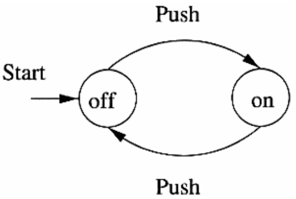
The machine only needs to remember “whether it is in the on state or off state." From this, we can infer that a state represents the relevant part of a machine’s history needed to predict a portion of the machine’s future behavior. This raises the question: “How to formalize this notion of state?" Computational mechanics addresses this by formalizing the concept probabilistically, defining it as a triple, as shown in Section 2.5.
Appendix B. Information Measures Across Varying Temperature in a Nearest-Neighbor Ising Model
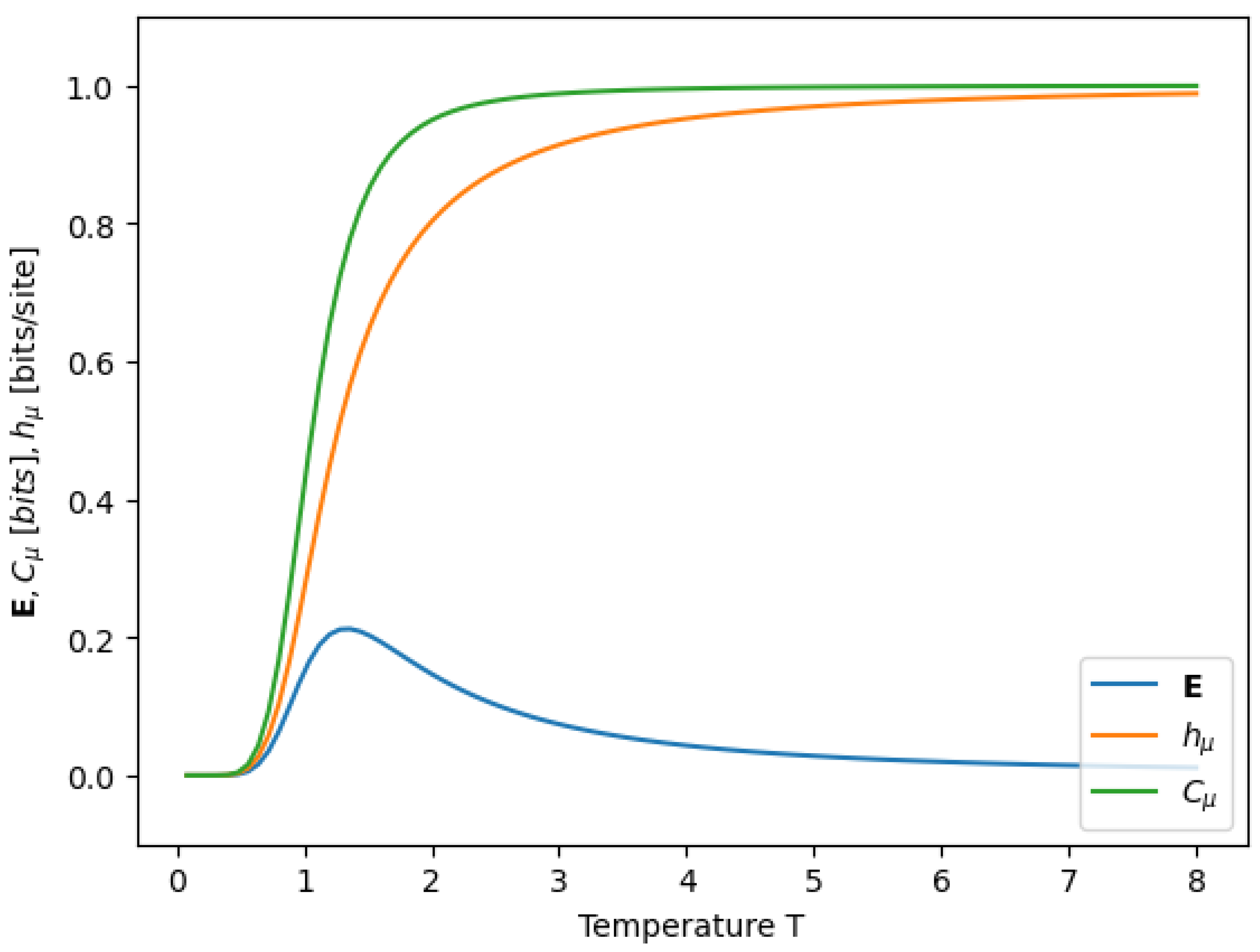
Figure A2 presents information measures , , and as functions of temperature T for a nn Ising model with and ferromagnetic coupling . This figure reproduces Figure 13 of Ref. [2].
Figure A2.
, , and v.s. T for nn spin- Ising model with and .
Appendix C. Shannon Entropy Density h μ and Boltzmann Entropy Density h therm
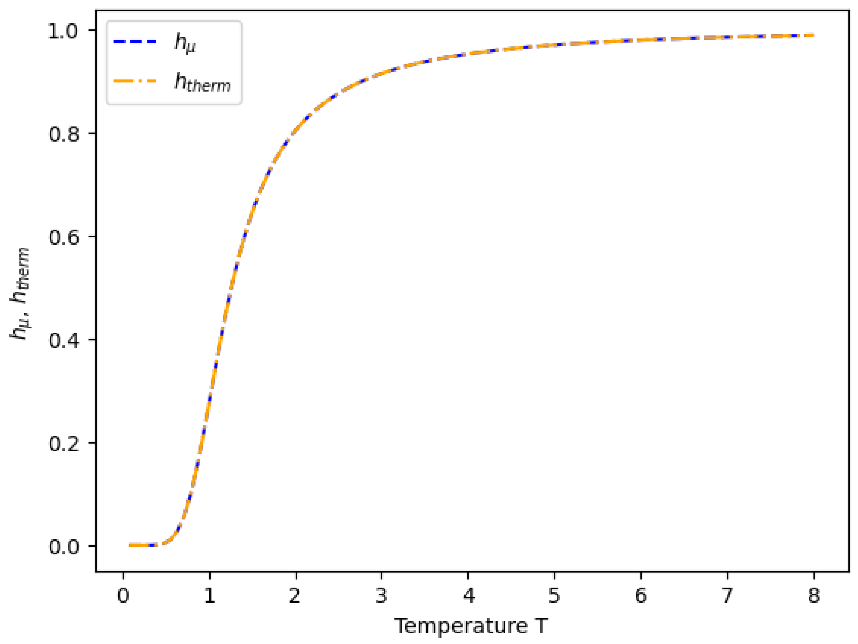
The form of the Boltzmann (thermodynamic) entropy density and Shannon entropy rate for a nn Ising model are presented in equations A1 and A2, respectively. These expressions are plotted as a function of temperature T in Figure A3, where they are graphically shown to be equivalent as temperature is varied.
Figure A3.
Boltzmann (thermodynamic) entropy density and Shannon entropy rate v.s. temperature T
Appendix D. Derivation of Boltzmann (Thermodynamic) Entropy Density for Nearest-Neighbor Ising Model
- Consider
- Using the chain rule:
- Rewrite in terms of
- Split principal eigenvalue into two terms
- Carry out and
- Simplify
- Simplify
- Simplify
- Replace in
Appendix E. ϵ-Machine of Nearest-Neighbor Ising Model
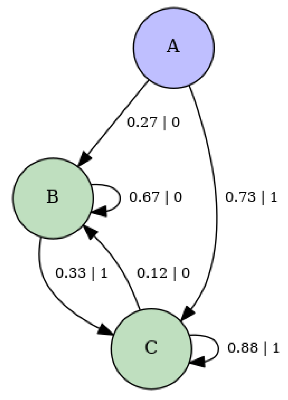
Figure A4 presents the -machine of a nearest-neighbor Ising model with , , and . This figure reproduces Figure 10 of Ref. [2].
Figure A4.
-machine of nn Ising model with , , and .
Appendix F. Joint Probability of Infinite Chain
- Consider a periodic infinite spin chain whose spins can only take two values (up or down) and only interact with their nearest neighbors.
- Define a Hamiltonian for this system in a translation-invariant manner.
- Calculate the system’s partition function.
- Define the Boltzmann probability of a given infinite configuration.
- Define the transfer matrix matrix, with components .
- Express Boltzmann probability weight in terms of transfer matrix components.
- Calculate partition function in the thermodynamic limit .
- Apply definition of matrix multiplication and enforce periodic boundary conditions .
- Apply definition of trace.
- Express joint probability of a given infinite spin chain in terms of principal eigenvalue and transfer matrix components .
Appendix G. Eigenvalue Decomposition of Transfer Matrix
- Express in terms of its eigenvalue decomposition .
-
Use fact that in the thermodynamic limit , . Rename as .Therefore,
- Express transfer matrix components in terms of the principal eigenvalue and the principal eigenvector components and at the thermodynamic limit.
Appendix H. Partition Function of Finite Chain with Fixed Boundary Conditions Embedded on Infinite Chain
Base Case ():
- Consider the partition function of a finite chain of length 3 with fixed boundary conditions.
- Express transfer matrix components in terms of principal eigenvalue and principal eigenvector components. For simplicity, we will drop the and , because for the nn Ising model the left and right eigenvectors are the same.
Inductive Step:
Appendix I. Joint Probability of Finite Chain Embedded on Infinite Chain
- Consider a finite spin chain embedded in an infinite spin chain.
-
The embedding of the finite spin chain implies:
- The thermodynamic limit applies to the finite chain.
- The magnetization is uniform across the bulk and boundaries of the finite chain.
- To ensure uniform magnetization, express in terms of conditional and marginal probabilities to separate the contributions from the bulk and boundaries. For simplicity, we denote as .
- Since and are independent, their probabilities can be factored as:
-
Express as a joint probability using .Thus,
- To recover Eq. (36), consider instead of
Appendix J. Finite-Range Ising Model Hamiltonian for R=1,2 and 3
The finite-range Ising model Hamiltonian is written below for neighborhood radii , , and . In the notation used for the Hamiltonian, the neighborhood radius R is denoted by n.
For :
For :
For :
Appendix K. Three-Body Model Transfer Matrix
The transfer matrix of the three-body spin model is shown in Eq. (A9). To simplify the notation of the matrix entries, we label each two-spin block as follows: , , , and . Moreover, we set the chemical potential to zero.
where
Note that, unlike the finite-range Ising model, the spin blocks in this model overlap by one spin. Specifically, the last spin in a row label must match the first spin in a column label. For example, the spin block in the second row can only transition to spin blocks or in the third and fourth columns, as its last spin ↓ matches the first spin of both and .
References
- S. Aaronson, S. M. Carroll, and L. Ouellette. arXiv 2014, arXiv:1405.6903.
- D. P. Feldman and J. P. Crutchfield, authors’ note: Manuscript completed in 1998 (Santa Fe Institute Working Paper 98-04-026). Entropy 2022, 24, 1282.
- Bak, P. How Nature Works: The Science of Self-organized Criticality; Springer New York: New York, 2013. [Google Scholar]
- J. Rothstein. Science 1951, 114, 171.
- I. Eliazar. Physica A: Statistical Mechanics and its Applications 2021, 568, 125662.
- J. M. Yeomans, Statistical Mechanics of Phase Transitions (Clarendon Press, Oxford, 1992).
- S. Krinsky and D. Furman. Physical Review B 1975, 11, 2602.
- R. Gheissari, C. R. Gheissari, C. Hongler, and S. C. Park. Communications in Mathematical Physics 2019, 367, 771. [Google Scholar]
- M. Schulz and S. Trimper. Journal of Statistical Physics 1999, 94, 173.
- R. H. Lacombe and R. Simha, The Journal of Chemical Physics 61, 1899 (1974).
- D. P. Landau and K. Binder, in A Guide to Monte Carlo Simulations in Statistical Physics (Cambridge University Press, Cambridge, United Kingdom, 2015) 4th ed., pp. 7–46.
- B. M. McCoy and T. T. Wu, Physical Review 176, 631 (1968).
- P. D. Beale, Physical Review Letters 76, 78 (1996).
- J. Köfinger and C. Dellago, New Journal of Physics 12, 093044 (2010).
- M. M. Tsypin and H.W. J. Blote, Physical Review E 62, 73 (2000).
- C. Chatelain and D. Karevski, Journal of Statistical Mechanics: Theory and Experiment 2006, P06005 (2006).
- R. K. Pathria and P. D. Beale, Statistical Mechanics, 3rd ed. (Butterworth-Heinemann, 2011).
- B. Derrida, Physical Review Letters 45, 79 (1980).
- M. Tribus, Thermostatics and Thermodynamics: An Introduction to Energy, Information and States of Matter, with Engineering Applications (D. Van Nostrand Company, Inc., Princeton, New Jersey, USA, 1961).
- G. Bateson, Steps to an Ecology of Mind: Collected Essays in Anthropology, Psychiatry, Evolution, and Epistemology (Jason Aronson Inc., Northvale, NJ and London, 1987).
- T. M. Cover and J. A. Thomas, Elements of Information Theory, 2nd ed. (Wiley-Interscience, Hoboken, NJ, USA, 2006).
- R. Shaw, The Dripping Faucet as a Model Chaotic System (Aerial Press, Santa Cruz, California, 1984).
- J. P. Crutchfield and N. H. Packard, Physica D 7, 201 (1983).
- P. Grassberger, International Journal of Theoretical Physics 25, 907 (1986).
- K. Lindgren and M. G. Nordhal, Complex Systems 2, 409 (1988).
- J. P. Crutchfield and K. Young, Physical Review Letters 63, 105 (1989).
- J. P. Crutchfield, Physica D 75, 11 (1994).
- J. P. Crutchfield, Nature Physics 8, 17 (2012).
- C. R. Shalizi and J. P. Crutchfield, Journal of Statistical Physics 104, 817 (2001).
- J. E. Hopcroft and J. D. Ullman, Introduction to Automata Theory, Languages, and Computation, 2nd ed. (Addison-Wesley, 2001).
- J. P. Crutchfield and C. R. Shalizi, Physical Review E 59, 275 (1999).
- S. Still, J. P. Crutchfield, and C. J. Ellison, CHAOS 20, 037111 (2010).
- C. C. Streloff and J. P. Crutchfield, Phys. Rev. E 89, 042119 (2014).
- S. E. Marzen and J. P. Crutchfield, Journal of Statistical Physics 163, 1312 (2016).
- A. Rupe, N. Kumar, V. Epifanov, K. Kashinath, O. Pavlyk, F. Schimbach, M. Patwary, S. Maidanov, V. Lee, Prabhat, and J. P. Crutchfield, in 2019 IEEE/ACM Workshop on Machine Learning in High Performance Computing Environments (MLHPC) (2019) pp. 75–87.
- A. Rupe and J. P. Crutchfield. arXiv 2020, arXiv:2010.05451.
- N. Brodu and J. P. Crutchfield, Chaos: An Interdisciplinary Journal of Nonlinear Science 32, 023103 (2022).
- A. M. Jurgens and N. Brodu, Chaos: An Interdisciplinary Journal of Nonlinear Science 35, 033162 (2025).
- D. P. Feldman and J. P. Crutchfield, Physical Review E 67, 051104 (2003).
- V. S. Vijayaraghavan, R. G. James, and J. P. Crutchfield, Santa Fe Institute Working Paper 15-10-042 (2016).
- C. Aghamohammadi, J. R. Mahoney, and J. P. Crutchfield, Scientific Reports 7, 6735 (2017).
- C. Aghamohammadi, J. R. Mahoney, and J. P. Crutchfield, Physics Letters A 381, 1223 (2017).
- P. Chattopadhyay and G. Paul. arXiv 2024, arXiv:2102.09981.
- D. Chu and R. E. Spinney, Interface Focus 8, 20180037 (2018).
- P. Strasberg, J. Cerrillo, G. Schaller, and T. Brandes. arXiv 2015, arXiv:1506.00894.
- D. H. Wolpert and J. Scharnhorst. arXiv 2024, arXiv:2410.07131.
- L. Li, L. Chang, R. Cleaveland, M. Zhu, and X. Wu. arXiv 2024, arXiv:2402.13469.
- A. S. Bhatia and A. Kumar. arxiv 2019, arXiv:1901.07992.
- D.-S. Wang. arXiv 2013, arXiv:1912.03767.
- A. Molina and J. Watrous, Proceedings of the Royal Society A: Mathematical, Physical and Engineering Sciences 475, 20180767 (2019).
- N. A. Alves, B. A. Berg, and R. Villanova, Physical Review B 41, 383 (1990).
- Y. Lin, F. Wang, X. Zheng, H. Gao, and L. Zhang, Journal of Computational Physics 237, 224 (2013).
- A. M. Ferrenberg, J. Xu, and D. P. Landau, Physical Review E 97, 043301 (2018).
- D. J. MacKay, Information Theory, Inference, and Learning Algorithms (Cambridge University Press, Cambridge, UK, 2003).
- A. V. Myshlyavtsev, in Studies in Surface Science and Catalysis, Vol. 138, edited by A. Guerrero-Ruiz and I. Rodríguez-Ramos (Elsevier Science B.V., Amsterdam, 2001) pp. 173–190.
- J. C. Flack, Philosophical Transactions of the Royal Society A: Mathematical, Physical and Engineering Sciences 375, 20160338 (2017).
- C. R. Shalizi and C. Moore, Foundations of Physics 55, 2 (2025).
- A. L. Ny. lectures given at the Semana de Mecânica Estatística, Universidade Federal de Minas Gerais and Universidade Federal do Rio Grande do Sul. arXiv 2007, arXiv:0712.1171.
- S. Muir, Nonlinearity 24, 2933 (2011).
- N. Ganikhodjaev, Journal of Mathematical Analysis and Applications 336, 693 (2007).
- D. Lind and B. Marcus, An Introduction to Symbolic Dynamics and Coding, second edition ed. (Cambridge University Press, Cambridge, United Kingdom, 2021).
- J. P. Crutchfield and D. P. Feldman, arXiv preprint cond-mat/0102181 (2001), santa Fe Institute Working Paper 01-02-012.
- C. E. Shannon and W. Weaver, The Mathematical Theory of Communication (University of Illinois Press, Champaign-Urbana, 1963).
- D. Feldman, A Brief Introduction to Information Theory, Excess Entropy, and Computational Mechanics, College of the Atlantic, Bar Harbor, ME (1998), revised October 2002.
- C. R. Shalizi, Causal Architecture, Complexity, and Self-Organization in Time Series and Cellular Automata, Ph.d. dissertation, University of Wisconsin-Madison, Madison, WI (2001), available at Santa Fe Institute: http://www.santafe.edu/~shalizi/thesis.
- S. E. Marzen and J. P. Crutchfield, Entropy 24, 90 (2022).
- K. Young and J. P. Crutchfield, Chaos, Solitons and Fractals 4, 5 (1994).
- K. A. Young, The Grammar and Statistical Mechanics of Complex Physical Systems, Ph.d. dissertation, University of California, Santa Cruz (1991).
- D. C. Dennett, The Journal of Philosophy 88, 27 (1991).
- R. Kikuchi, Physical Review 99, 1666 (1955).
- J. F. Dobson, Journal of Mathematical Physics 10 (1969).
- M. Slotnick, Physical Review 83, 996 (1951).
- C. Zener and R. R. Heikes, Reviews of Modern Physics 25, 191 (1953).
- A. V. Zarubin, F. A. Kassan-Ogly, A. I. Proshkin, and A. E. Shestakov, Journal of Experimental and Theoretical Physics 128, 778 (2019).
- K. A. Mutallib and J. H. Barry, Physical Review E 106, 014149 (2022).
- R. Moessner and S. L. Sondhi, Physical Review B 63, 224401 (2001).
- W. K. Burton, N. Cabrera, and F. C. Frank, Philosophical Transactions of the Royal Society of London. Series A, Mathematical and Physical Sciences 243, 299 (1951).
- J. D. Weeks, in Ordering in Strongly Fluctuating Condensed Matter Systems, NATO Advanced Study Institutes Series: Series B, Physics, Vol. 50, edited by T. Riste (Plenum Press, New York, 1980) pp. 293–315.
- V. Privman and N. M. Švrakić, Journal of Statistical Physics 51, 819 (1988).
- D. B. Abraham, Department of Mathematics, University of Newcastle, Newcastle, New South Wales 2308, Australia (1979).
- J. Wang, X. Feng, C. W. Anderson, Y. Xing, and L. Shang, Journal of Hazardous Materials 221, 1 (2012).
- J. D. Aparicio, E. E. Raimondo, J. M. Saez, S. B. Costa-Gutierrez, A. Alvarez, C. S. Benimeli, and M. A. Polti, Journal of Environmental Chemical Engineering 10, 107141 (2022).
- V. P. Zhdanov, Surface Science 111, 63 (1981).
- P. A. Redhead, Vacuum 12, 203 (1962).
- M. A. Morris, M. Bowker, and D. A. King, in Comprehensive Chemical Kinetics, Vol. 19 (Elsevier, 1984) pp. 1–179.
- V. P. Zhdanov and K. I. Zamaraev, Soviet Physics Uspekhi 29, 755 (1986).
- A. V. Myshlyavtsev, J. L. Sales, G. Zgrablich, and V. P. Zhdanov, Journal of Chemical Physics 91, 7500 (1989).
| 1 | This paper uses two notions of structure. One refers to a system’s general type of arrangement, which we call generic structure. The other captures a more specific type of arrangement—one that exhibits patterns—which we call intrinsic structure. Throughout the paper, the intended notion will be clear from context. |
| 2 | |
| 3 | Without loss of generality |
| 4 | It should be highlighted that for 1D spin lattice models, the conventional time index is taken to be site location index and there is no time dependence. |
| 5 | This principle formalizes the implicit definition of a state commonly used in theoretical computer science when constructing machines. In this context, a state represents the information that must be retained to predict the system’s future behavior (see Appendix A). |
| 6 | To avoid accounting for computation not inherent to our system |
| 7 | In the 21st century, “computation” often evokes laptops, which perform useful computation—that is, computation carried out for some external task. In contrast, we focus on intrinsic computation, the computation a system performs by itself. To analyze this, we use abstract machines [30]—mathematical models that consist of states and transitions and laid the groundwork for theory of computation. |
Figure 1.
Depiction of a finite spin configuration embedded within an infinite spin configuration with periodic boundary conditions
Figure 1.
Depiction of a finite spin configuration embedded within an infinite spin configuration with periodic boundary conditions
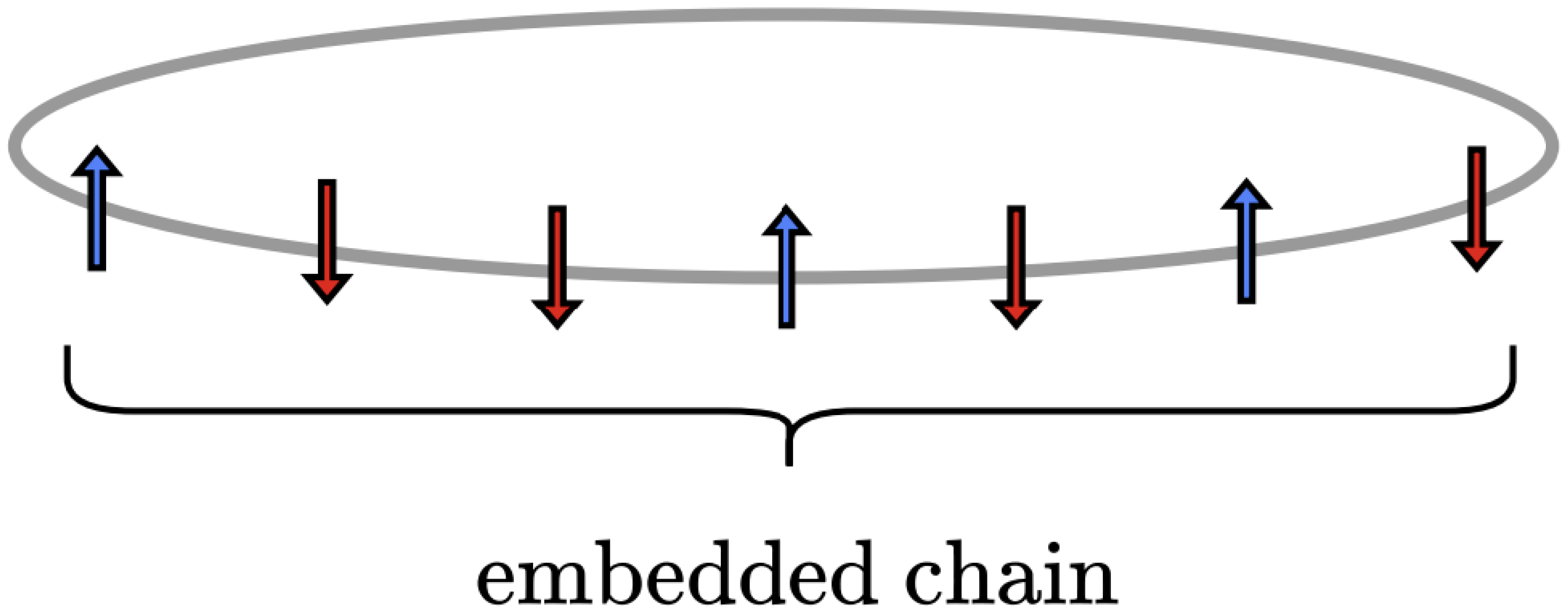
Figure 2.
Graphical representation of coarse–grained Ising phase space. Only the purple spins are assigned fixed indices. For clarity, down spins ↓ are represented as 0 instead of .
Figure 2.
Graphical representation of coarse–grained Ising phase space. Only the purple spins are assigned fixed indices. For clarity, down spins ↓ are represented as 0 instead of .
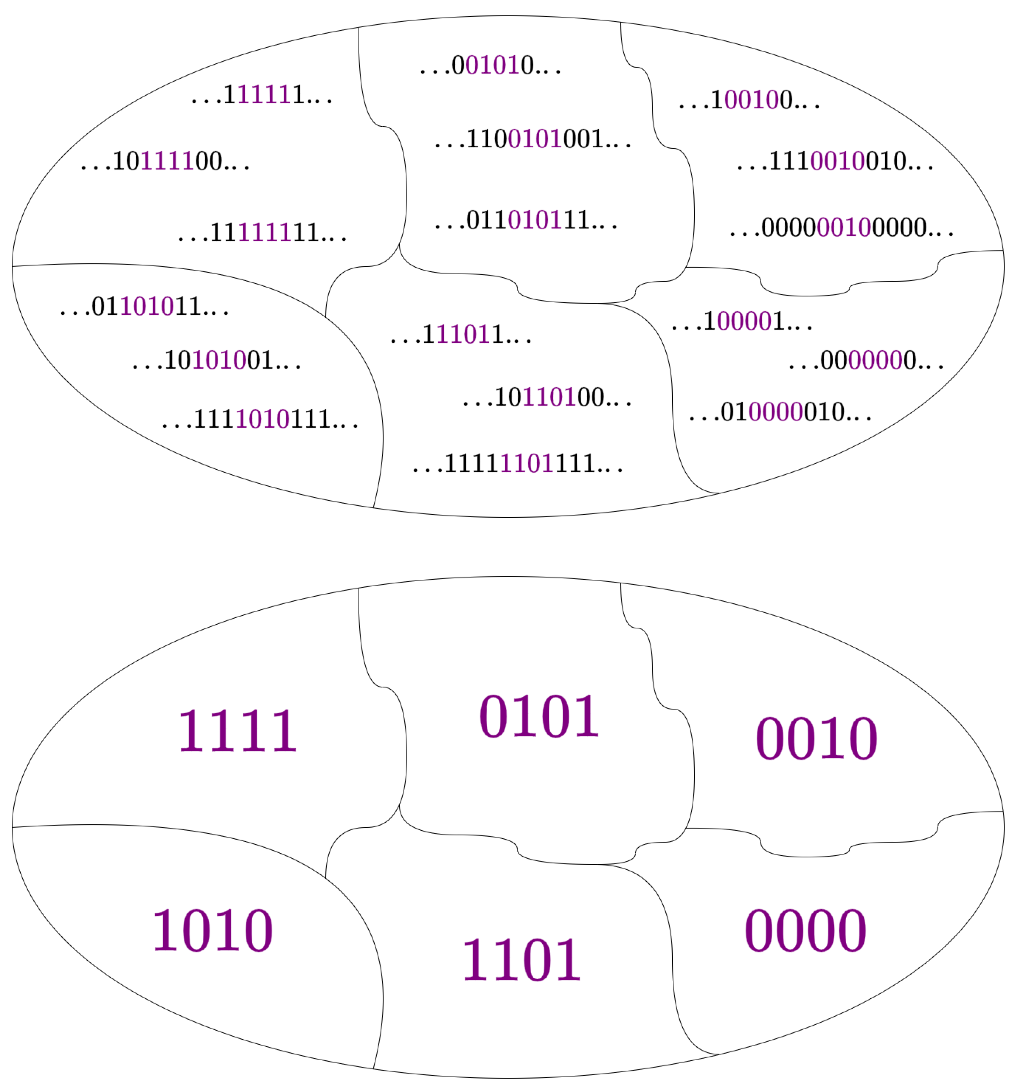
Figure 3.
Graphical representation of configuration and ensemble pattern concepts.
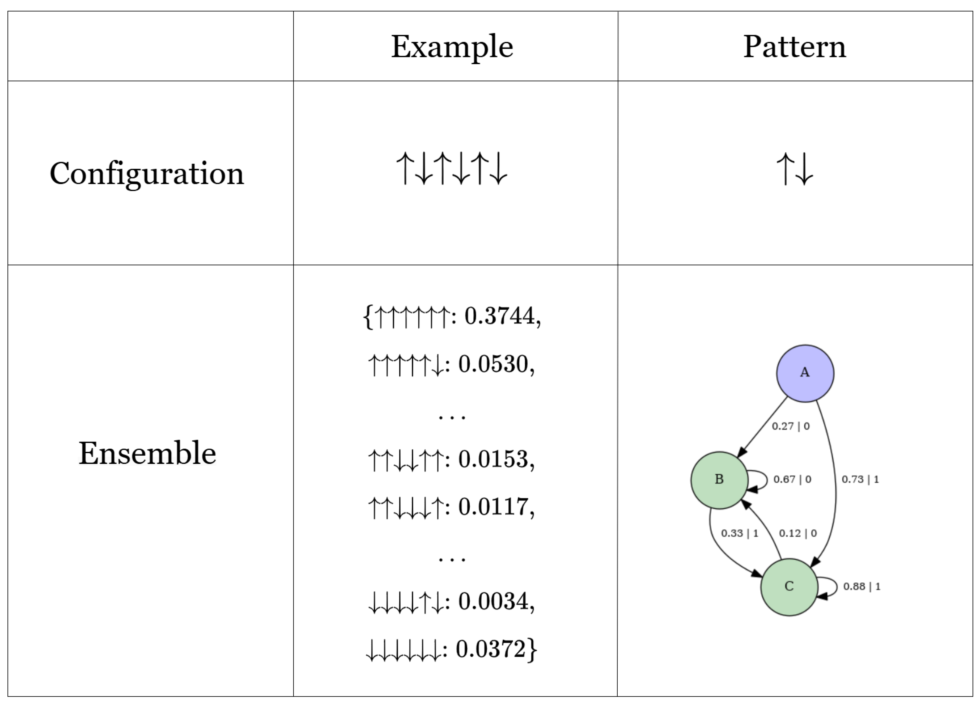
Figure 4.
Illustration of spin interactions in Ising models with neighboring radii (top), (middle), and (bottom)
Figure 4.
Illustration of spin interactions in Ising models with neighboring radii (top), (middle), and (bottom)
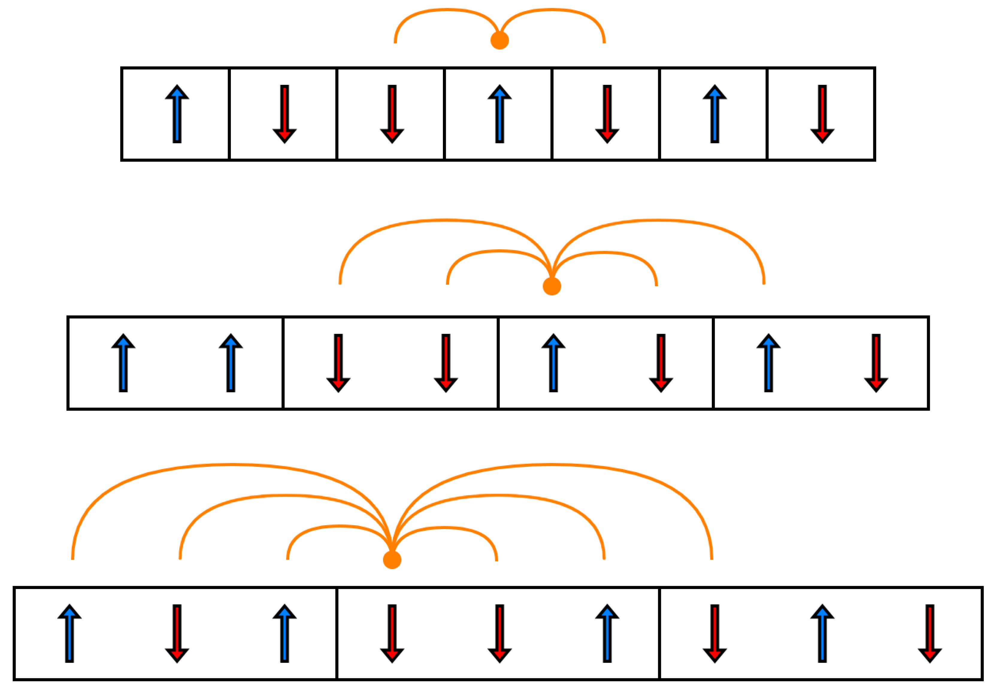
Figure 5.
(a) , E and v.s. for nnn Ising model with , and . (b) , E and v.s. B for 3-range Ising model with , , and .
Figure 5.
(a) , E and v.s. for nnn Ising model with , and . (b) , E and v.s. B for 3-range Ising model with , , and .
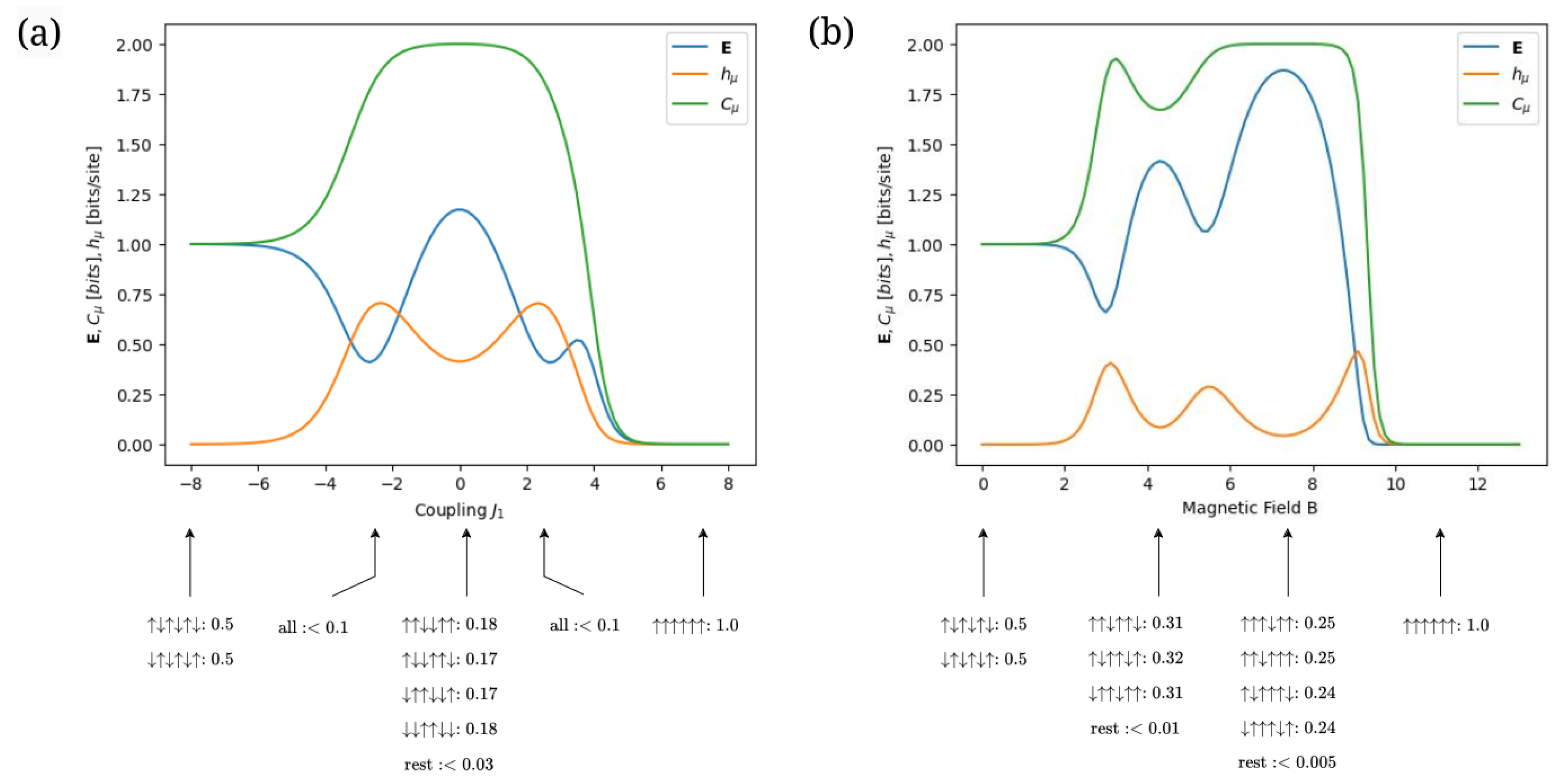
Figure 6.
(a) -machine of 3-range Ising model with , , , and . (b) -machine of 3-range Ising model with , , , and .
Figure 6.
(a) -machine of 3-range Ising model with , , , and . (b) -machine of 3-range Ising model with , , , and .
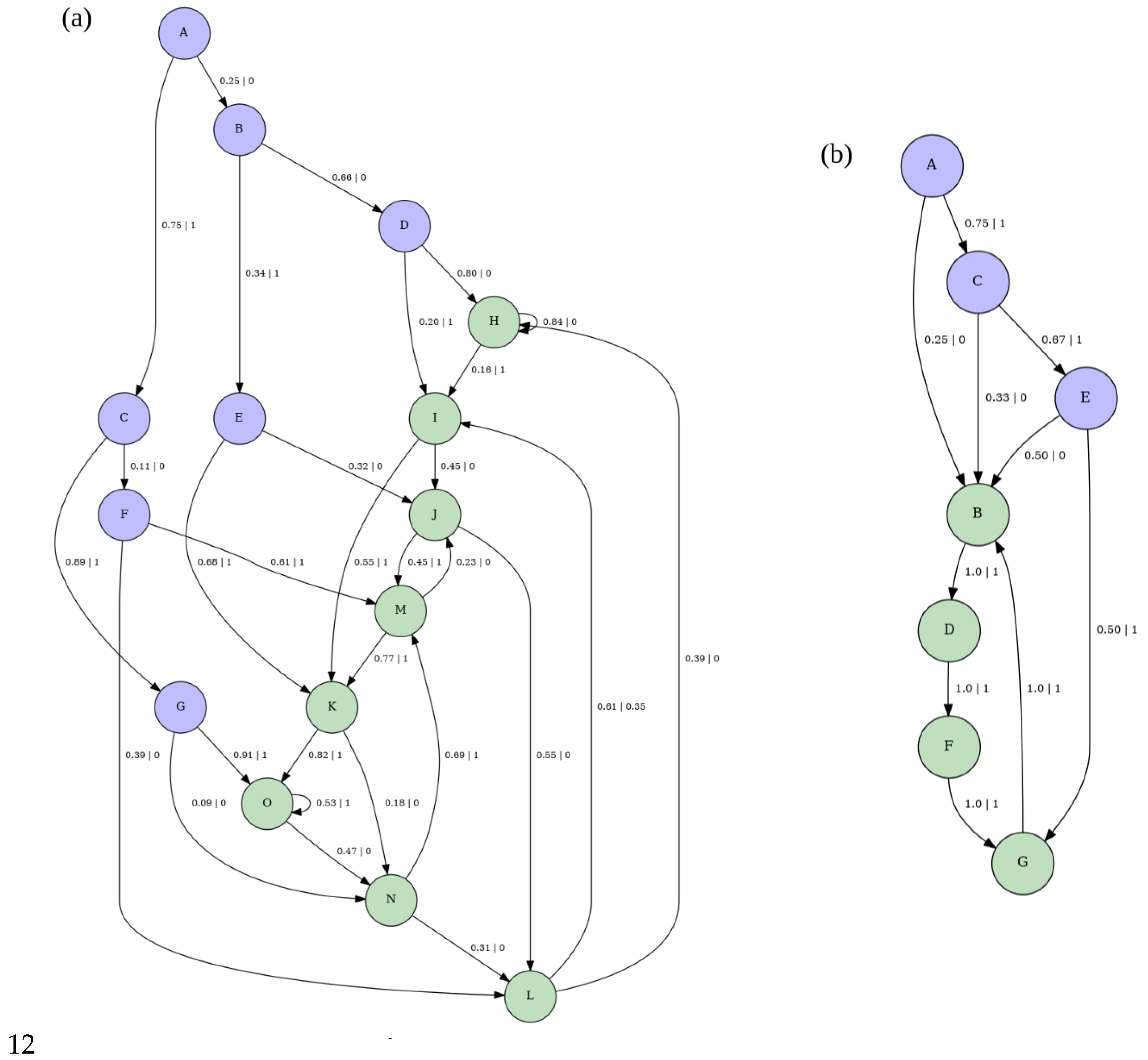
Figure 7.
Illustration of spin interactions in a 2D spin lattice with the leftmost and rightmost spins fixed to opposite values. The dashed black lines highlight the induced 1D spin chain interface.
Figure 7.
Illustration of spin interactions in a 2D spin lattice with the leftmost and rightmost spins fixed to opposite values. The dashed black lines highlight the induced 1D spin chain interface.
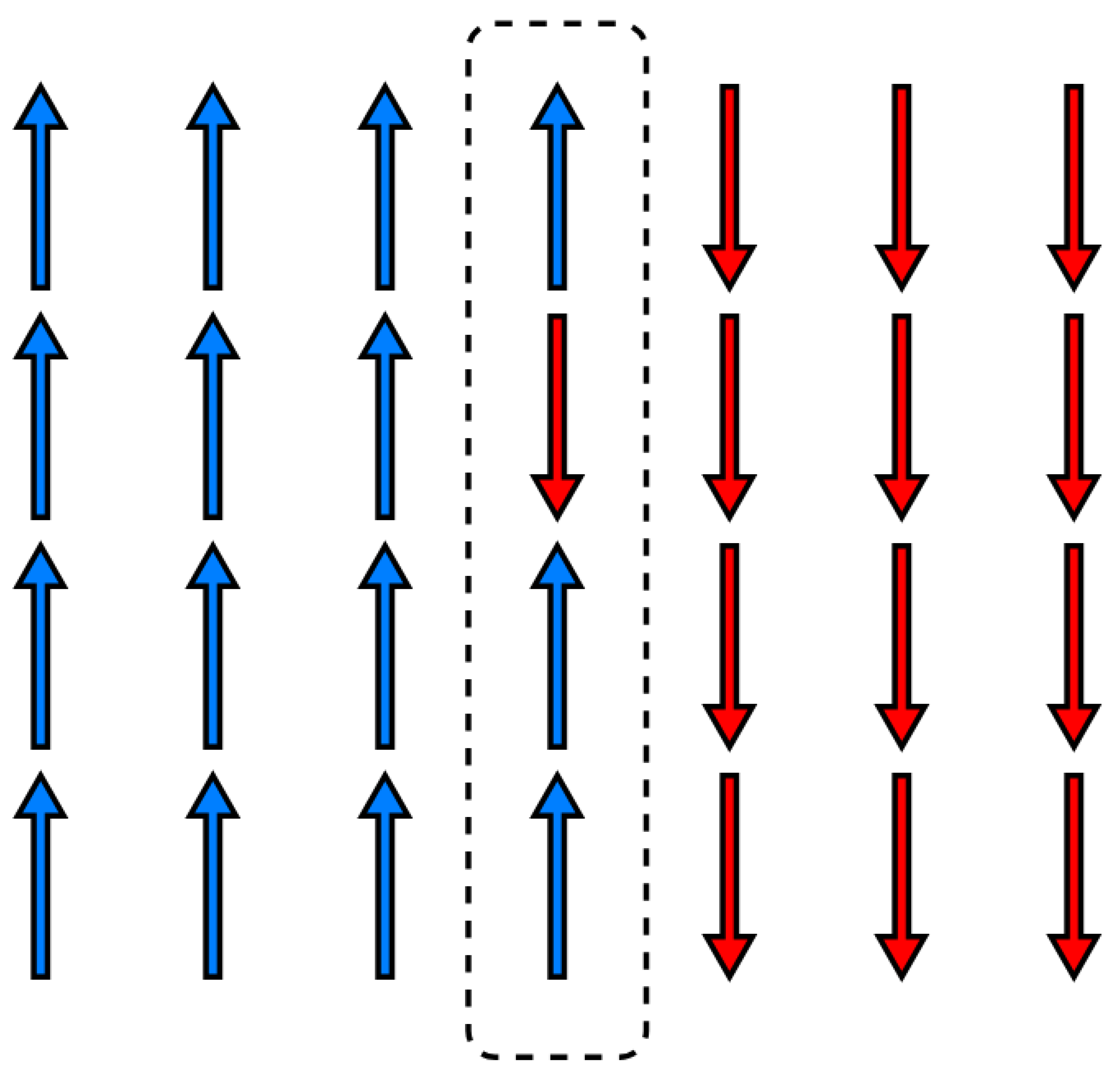
Figure 8.
(a) , and v.s. U for SOS model with , and . (b) , and v.s. U for SOS model with , and .
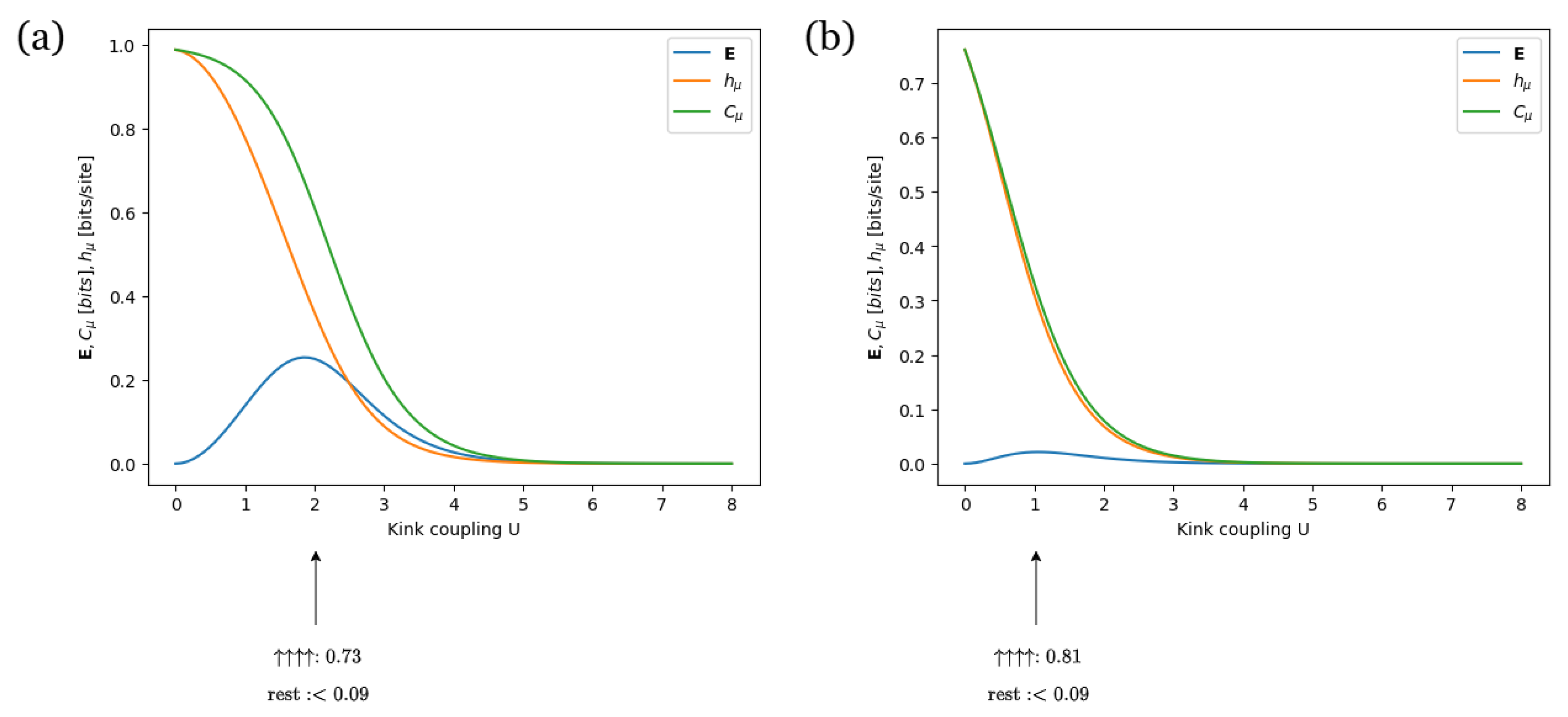
Figure 9.
(a) -machine for SOS model with , , , and . (b) -machine for SOS model with , , , and .
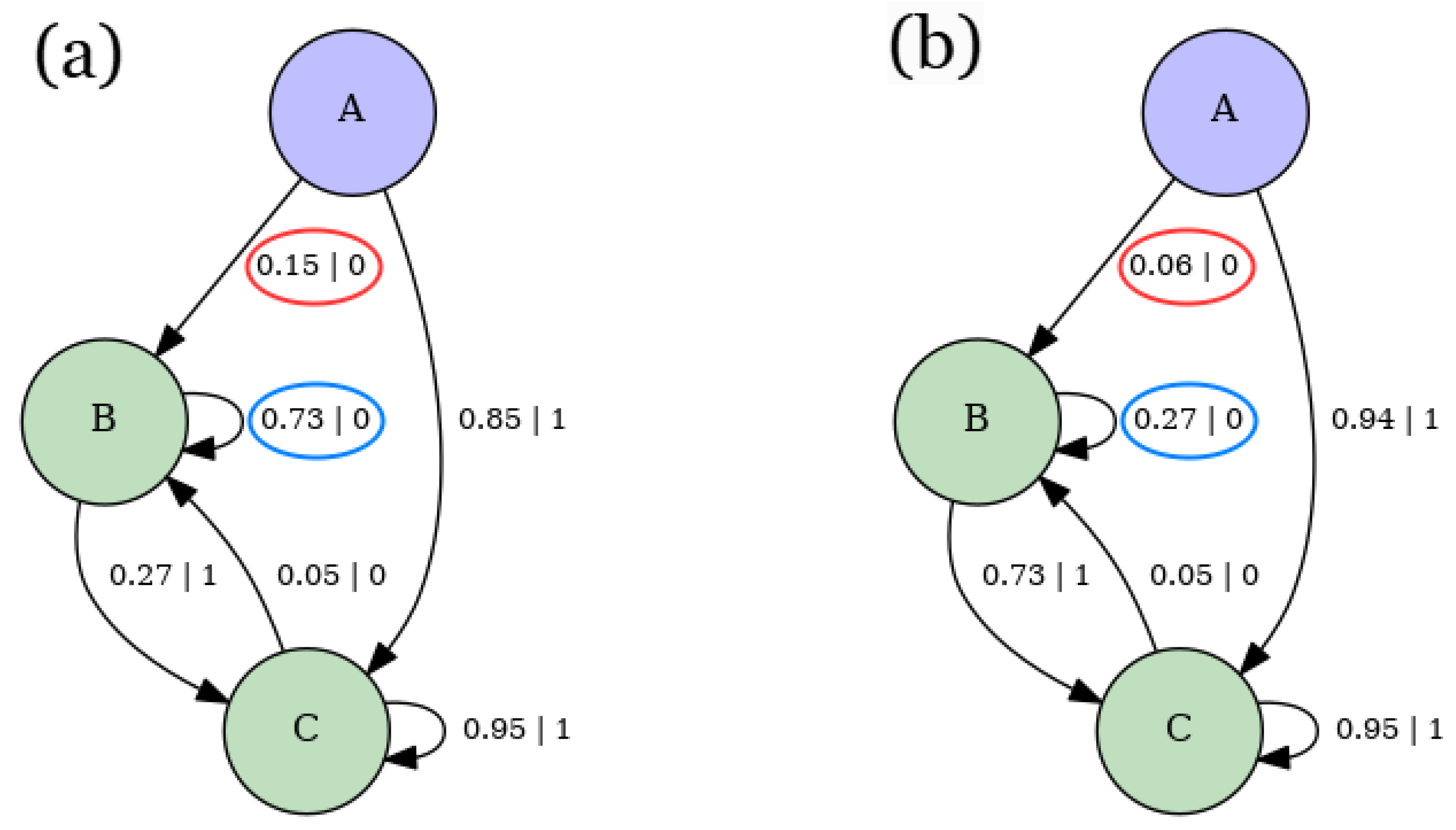
Figure 10.
Illustration of spin interactions in three-body models: nearest-neighbor (purple), next-nearest neighbor (green), and three-body (orange) interactions.
Figure 10.
Illustration of spin interactions in three-body models: nearest-neighbor (purple), next-nearest neighbor (green), and three-body (orange) interactions.

Figure 11.
(a) , and v.s. T for three body model with , and . (b) , and v.s. T for three body model with , and .
Figure 11.
(a) , and v.s. T for three body model with , and . (b) , and v.s. T for three body model with , and .
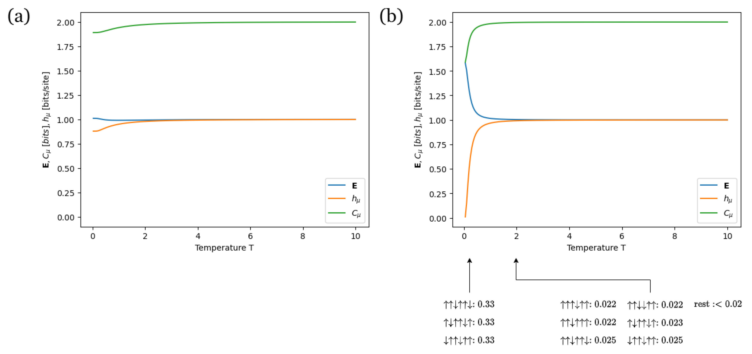
Figure 12.
(a) -machine for three body model with , , , . (b) -machine for three body model with , , ,
Figure 12.
(a) -machine for three body model with , , , . (b) -machine for three body model with , , ,
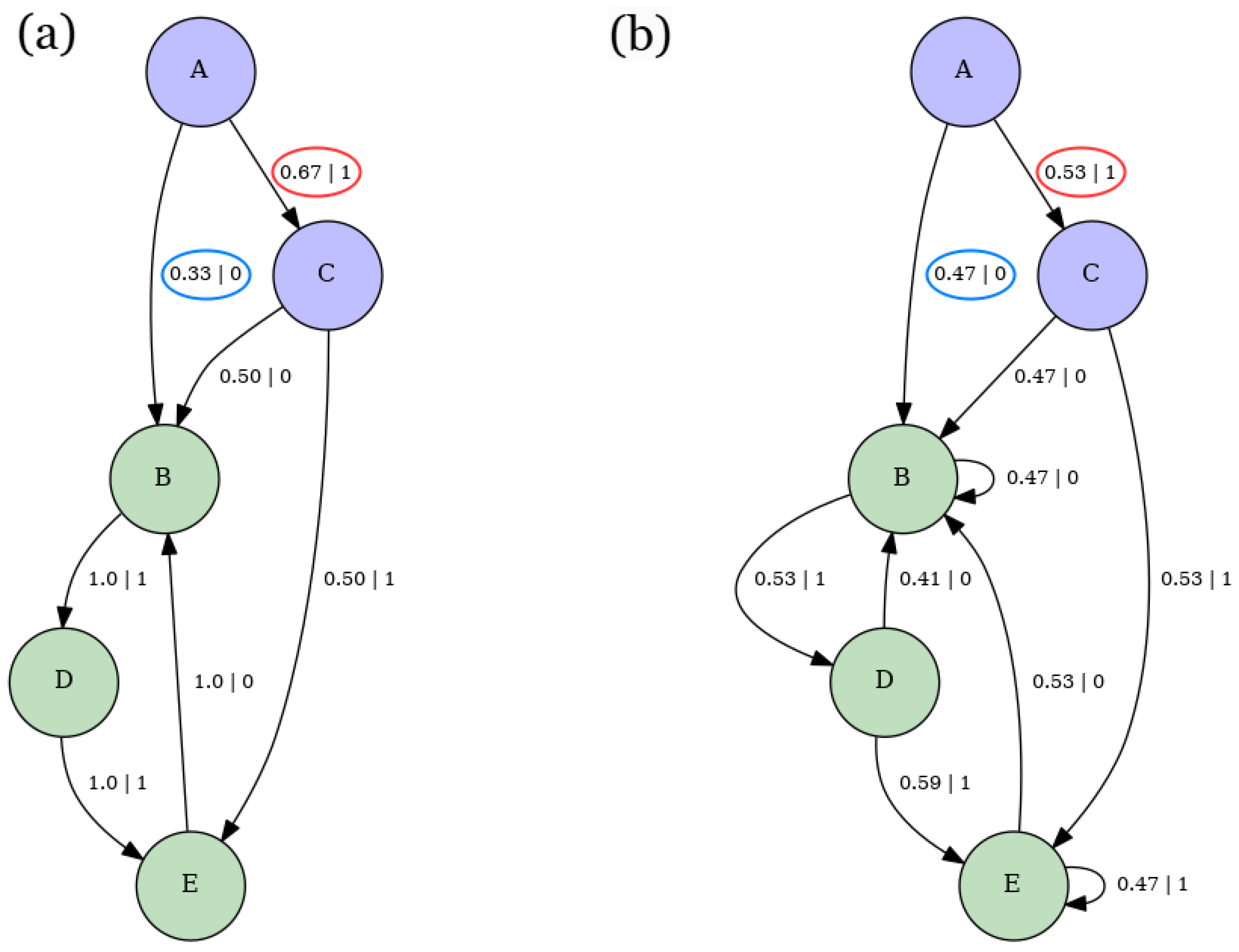
Disclaimer/Publisher’s Note: The statements, opinions and data contained in all publications are solely those of the individual author(s) and contributor(s) and not of MDPI and/or the editor(s). MDPI and/or the editor(s) disclaim responsibility for any injury to people or property resulting from any ideas, methods, instructions or products referred to in the content. |
© 2025 by the authors. Licensee MDPI, Basel, Switzerland. This article is an open access article distributed under the terms and conditions of the Creative Commons Attribution (CC BY) license (http://creativecommons.org/licenses/by/4.0/).
Copyright: This open access article is published under a Creative Commons CC BY 4.0 license, which permit the free download, distribution, and reuse, provided that the author and preprint are cited in any reuse.


