Submitted:
17 October 2025
Posted:
17 October 2025
You are already at the latest version
Abstract
Ocean surface wind vector (OWV) is a key variable for ocean remote sensing and tropical cyclone (TC) monitoring. This study presents the first comprehensive intercomparison of Ku-band OWV products from FY-3E/WindRAD and HY-2B/SCA scatterometers using full-year 2022 data (583,805 spatiotemporal collocations), with both sensors sampling the morning–evening local-time sector in sun-synchronous orbits. Results indicate strong agreement in wind speed (R = 0.95; mean bias −0.47 m s⁻¹; RMSE 1.30 m s⁻¹) and wind direction (mean bias −0.47°; SD 33.7°; most differences within ±20°), with the highest consistency across Beaufort scale 3–8 (B3–B8). A fusion leveraging FY-3E’s fine resolution and HY-2B’s wide coverage is implemented and applied to Super Typhoon Hinnamnor (2022), enhancing spatial coverage and structural detail of TC winds. Quadrant 34-kt wind radii (R34) are estimated from fused fields and evaluated against Joint Typhoon Warning Center (JTWC) best-tracks data, showing close agreement during compact, symmetric TC stages but larger differences during structural reorganization. Overall, the findings confirm inter-satellite consistency for the two Chinese scatterometers and demonstrate the practical value of a multi-source fusion approach that benefits TC mon-itoring, wind-radii estimation, and marine weather services.
Keywords:
ocean surface wind vector (OWV)
; FY-3E WindRAD
; HY-2B SCA
; scatterometer
; intercomparison and validation
; multi-satellite fusion
; tropical cyclone monitoring
; wind-radii estimation
; R34
; ocean remote sensing
1. Introduction
Ocean surface wind vector (OWV) is an essential geophysical parameter in meteorology, ocean dynamics, and climate studies, and is critical for tropical-cyclone monitoring, numerical weather prediction, offshore wind-energy assessment, and marine-engineering safety. [1,2]. Conventional in situ measurements from buoys and ships are constrained by sparse spatial and temporal coverage, making them inadequate for continuous global monitoring [3,4]. By contrast, satellite-based remote sensing, particularly active microwave scatterometry, provides high-resolution, all-weather, and wide-area observations of global ocean surface winds[5,6].
Since the Seasat satellite first carried the Seasat-A Satellite Scatterometer (SASS) in the late 1970s [7,8], the international ocean wind observing system has developed rapidly, with successive generations of scatterometers such as the AMI-SCAT on ERS-1/2 [9], NSCAT on ADEOS-I [10,11], SeaWinds on QuikSCAT [12], ASCAT on MetOp [13], OSCAT on OceanSat, and CFOSCAT on CFOSat. These missions have collectively advanced global wind observations and highlighted the value of scatterometer data for weather analysis, data assimilation, and marine forecasting[14,15,16,17,18,19,20,21,22,23].
In recent years, China has made significant progress in spaceborne wind observations. The Fengyun-3E (FY-3E), launched in July 2021, carries the WindRAD, China’s first operational dual-frequency (Ku/C-band), dual-polarization, conically scanning scatterometer. This instrument enhances global OWV monitoring and provides critical data for dawn–dusk orbit meteorology [24,25]. Validation studies have demonstrated good wind speed and direction accuracy for FY-3E/WindRAD [26,27,28,29] . Meanwhile, the Haiyang-2B (HY-2B) satellite, launched in October 2018 for dynamic ocean environment monitoring, is equipped with a microwave scatterometer (SCA), one of China’s first operational Ku-band instruments [30] . Its wind products have shown high reliability and broad applicability through multi-source validation[31,32,33,34], and intercomparison with international scatterometers (e.g., ASCAT, OSCAT) has further confirmed the consistency of its wind observations [32,35,36] . However, no systematic intercomparison between FY-3E/WindRAD and HY-2B/SCA has yet been conducted.
FY-3E and HY-2B both operate in sun-synchronous orbits, with nearly coincident overpass times (within about 30 minutes), and both provide Ku-band wind vector products. This enables high-precision spatiotemporal collocation and intercomparison. Their observing capabilities are complementary: FY-3E/WindRAD offers higher spatial resolution, capturing wind gradients in tropical cyclone (TC) cores and high-wind regions, while HY-2B/SCA, with its wider swath, provides broader spatial coverage that captures the overall TC structure[37,38,39]. Intercomparison of these sensors not only allows objective evaluation of FY-3E/WindRAD data quality and stability but also reveals the impacts of different system designs (e.g., dual-/single-frequency, scanning geometry, retrieval algorithms)[40,41] on wind product consistency.
In the context of multi-satellite constellation observations, data fusion has become an effective strategy for filling observation gaps, improving spatial continuity, and enhancing extreme weather monitoring capability[42,43]. While fusion methods have been widely applied to international scatterometers (e.g., ASCAT, SeaWinds)[44,45], the integration of FY-3E/WindRAD and HY-2B/SCA products remains underexplored. To address this gap, this study conducts the first systematic intercomparison of Ku-band wind speed and direction products from FY-3E/WindRAD and HY-2B/SCA using full-year 2022 data. Furthermore, the potential of near-synchronous dual-satellite fusion is assessed using a case study of Super Typhoon Hinnamnor (2022), with emphasis on its utility for enhanced TC monitoring and refined wind-radii estimation[46,47,48].
2. Materials and Methods
2.1. Data
The WindRAD onboard FY-3E is China’s first operational dual-frequency (Ku/C-band) conically scanning scatterometer with dual-polarization capability. It has swath widths of 1300 km/1250 km and provides wind products at spatial resolutions of 10 km and 25 km, with an effective wind speed range of 3–40 m/s[49]. In this study, the Ku-band product (WRADKu, central frequency 13.256 GHz) is used, which is stored in HDF5 format and publicly available from the National Satellite Meteorological Center (https://data.nsmc.org.cn). The scatterometer (SCA) onboard the Haiyang-2B (HY-2B) satellite is one of China’s first operational Ku-band fan-beam scatterometers. Its Level-2B wind field product has a spatial resolution of 25 km, also with a central frequency of 13.256 GHz, and is distributed by the National Satellite Ocean Application Service (https://osdds.nsoas.org.cn). The dataset, in HDF5 format, contains wind speed, wind direction, observation time, geolocation, and quality control information [50] .
Based on these Level-2 products, this study uses one year of observations (1 January–31 December 2022), focusing on the Northwest Pacific and adjacent seas of China, to conduct consistency evaluation and error structure analysis of Ku-band wind products from the two satellites. Despite differences in polarization, scanning geometry, and retrieval algorithms [18,51,52,53,54,55] (Table 1), unified quality control and pixel selection criteria were applied to ensure scientific rigor and comparability. Figure 1 illustrates typical spatial coverage and wind field structures from both satellites.
The TC information used in this study is obtained from the IBTrACS v4 (International Best Track Archive for Climate Stewardship) best-track dataset, which integrates records from multiple agencies such as JTWC and CMA, providing global coverage and standardized sources (data access: https://www.ncei.noaa.gov/products/international-best-track-archive). From IBTrACS, the JTWC best track is extracted as the reference for evaluating TC center positions and wind-radii, including variables such as center location, intensity, maximum sustained wind, minimum sea-level pressure, and quadrant wind radii (e.g., R34/R50). Specifically, IBTrACS v4 provides a 3-hourly series interpolated from the 6-hourly source analyses[56]. Positions are interpolated using splines, whereas non-position variables (e.g., winds, pressure, and quadrant radii) are interpolated linearly, which facilitates precise time matching with satellite overpasses and a finer depiction of TC evolution.
2.2. Methods
2.2.1. Data Preprocessing
To ensure the scientific validity and comparability of the intercomparison, strict quality control procedures were applied. Pixels flagged as invalid due to retrieval failure, GMF fitting anomalies, sea ice contamination, land contamination, rainfall effects, or insufficient sigma-0 were removed, while physically reasonable high-wind and low-wind observations were retained. Edge pixels from the first two and last two columns of both satellites were discarded to avoid scan distortions. Wind speed values were converted from raw storage units (e.g., 0.01 m/s) to standard SI units (m/s). All subsequent analyses were based on these quality-controlled datasets.
2.2.2. Spatiotemporal Collocation
Intercomparison between FY-3E/WindRAD and HY-2B/SCA was performed using a nearest-neighbor matching method constrained by temporal and spatial windows, considering orbit proximity, resolution, and operational feasibility.
- Temporal matching: FY-3E and HY-2B are both in sun-synchronous orbits with local equator crossing times of 05:30/17:30 and 06:00/18:00, respectively. Their observation time difference is typically within ±30 min. Accordingly, a temporal window of ±30 min was applied, and only collocated orbits within this interval were retained.
- Spatial matching: Taking FY-3E/WindRAD pixels as the reference, the nearest neighbor in HY-2B/SCA was identified using great-circle distance. Pairs with separation less than 25 km (corresponding to the scatterometer footprint) were retained. The great-circle distance was calculated as follows:
To further avoid degraded quality at swath edges, the outermost two rows and columns of both datasets were removed.
- Wind direction normalization: To resolve 360° periodic ambiguity, wind direction differences were normalized to the [−180°, +180°] interval:
where are wind directions from FY-3E/WindRAD and HY-2B/SCA.
The resulting collocated dataset includes matched wind speeds, wind directions, and geolocation from both satellites, providing high-consistency samples for inter-sensor validation.
2.2.3. Evaluation Metrics
To assess consistency, multiple statistical metrics were applied to matched wind speed and direction samples.
- Wind speed metrics: Mean Bias, Root Mean Square Error (RMSE), Mean Absolute Error (MAE), and Pearson correlation coefficient (R).
- Wind direction metrics: Mean Bias, Standard Deviation (Std), Median Bias, and Median Absolute Bias.
Bias reflects systematic deviation, RMSE and MAE measure overall dispersion, and Revaluates linear consistency. Wind direction metrics capture angular difference distributions under circular conditions. These indicators are widely used in wind field validation [57,58].
Furthermore, wind speed differences were stratified by Beaufort scale based on HY-2B/SCA as the reference (Table 2). This enabled evaluation of FY-3E/WindRAD performance across weak, moderate, and high wind conditions.
2.2.4. Satellite Data Fusion
To enhance spatial coverage and structure reconstruction of wind fields under extreme weather, a fusion experiment was conducted using Typhoon Hinnamnor (No. 2211) as a case study. The procedure included:
- Quality control and preprocessing. Both datasets underwent unified quality control to remove retrieval failures, precipitation, and land contamination.
- Sample selection. Only pixels with wind speed ≥10.8 m/s (Beaufort scale 6 or higher) were retained to focus on TC core structures and reduce low-wind noise.
- Resolution harmonization and fusion. HY-2B/SCA data were resampled to 10 km resolution, consistent with FY-3E/WRADKu. FY-3E was given priority, with HY-2B used to fill uncovered areas. Spatial tolerance was set to 0.06° (~6 km), approximately half of the native FY-3E/WindRADKu footprint. This value balances collocation density and representativeness errors, and is consistent with commonly adopted spatial collocation windows in previous scatterometer validation and intercomparison studies [58,59].
2.2.5. Estimation of Wind Radius (R34) and Comparison with JTWC
This study focuses on estimating the 34-kt wind radius (R34). In operations,R50/R64 are often inferred from statistical/parameterized relations with R34 and intensity, whereas R34 can be directly and robustly extracted from the fused wind field. TC centers are taken from IBTrACS v4, prioritizing JTWC fixes (CMA as fallback). JTWC best-track analyses are issued at 6-hour synoptic times (00/06/12/18 UTC). For time matching, the 3-hourly IBTrACS v4 series is used; off-synoptic timestamps (e.g., 09:00 or 21:00 UTC) therefore correspond to IBTrACS interpolations rather than original JTWC analyses. Fused snapshots are paired with best tracks within ±45 min to cover the ~30-min orbit offset and edge/interpolation effects; the implied translation (~27–54 km) is small relative to the collocation radius (~25 km), grid spacing (10 km), and the R34 scale (100–300 km). Using the matched center as origin, grid points are partitioned into NE/SE/SW/NW quadrants. For points exceeding 34 kt (17.5 m s⁻¹), great-circle distances to the center are computed per equation (1); the quadrant radius is taken as the P90 of those distances, capped at 500 km (rmax) and requiring at least 10 samples (minN); if insufficient, a first-exceedance/min-distance fallback is applied. If samples are insufficient, a first-exceedance/min-distance fallback is ap-plied. Validation time-matches quadrantwise R34 to JTWC radii (units harmonized via 1 nm = 1.852 km) and reports Bias and RMSE, with Bias (km) defined as
and the relative bias defined as
Here, is the estimate and is the reference.
3. Results
Based on the aforementioned quality control and spatiotemporal collocation methods, this study systematically evaluates the consistency of Ku-band wind field products from FY-3E/WindRAD and HY-2B/Scatterometer (SCA). The results section focuses on statistical analyses of wind speed and wind direction, exploring key factors that influence the agreement between the two satellite products. In addition, a representative case of data fusion is presented to illustrate the complementary strengths of the two sensors during a typhoon event.
3.1. Wind Speed Comparison
Using pixel-level collocated data from the entire year of 2022, a total of 583,805 valid pairs of wind speed observations were obtained. The results (Figure 2) show a high level of agreement between the two sensors, with a Pearson correlation coefficient (R) of 0.95, a mean bias of −0.47 m/s, and a root mean square error (RMSE) of 1.30 m/s. These values indicate that the wind speed retrieved by FY-3E is slightly lower than that from HY-2B. The slope and intercept of the least squares regression line are 0.89 and 0.46 m/s, respectively, suggesting a systematic underestimation by FY-3E in the moderate to high wind speed range. Most of the sample points are densely distributed around the 1:1 reference line, with only a small number of outliers. Overall, the two wind speed products exhibit good consistency and high operational applicability across the primary wind speed range.
To further characterize the statistical distribution of differences between FY-3E/WRADKu and HY-2B/SCA wind speeds, a probability density function (PDF) analysis was conducted (Figure 3). Consistent with the results above, FY-3E/WRADKu tends to underestimate wind speeds relative to HY-2B/SCA. The median bias is −0.30 m/s, and the standard deviation is 1.21 m/s. The skewness and kurtosis are −1.09 and 8.80, respectively, indicating a sharp-peaked, heavy-tailed distribution with a slight leftward skew. Most of the differences lie within ±3 m/s, with a minimum of −19.90 m/s and a maximum of 10.70 m/s. These few extreme outliers have limited impact on the overall distribution. In summary, the FY-3E/WRADKu and HY-2B/SCA products demonstrate good consistency within the main operational range, although slight negative biases and a small number of large negative deviations are present in the FY-3E/WRADKu product.
3.1.1. Bias Under Different Wind Speeds
To assess wind speed differences under various wind conditions, the collocated samples from 2022 were categorized according to the Beaufort wind scale (B0–B12). Figure 4 presents the mean bias and standard deviation (±1σ) of wind speed differences between FY-3E/WRADKu and HY-2B/SCA across all Beaufort levels, along with the corresponding number of samples per category (right y-axis).
The majority of samples are concentrated in the moderate wind force range (B3–B6, 3.4–13.8 m/s), accounting for over 48% of the total. Specifically, the B4 and B5 categories contain 147,074 and 141,174 matched samples, respectively, with mean biases within ±0.25 m/s and standard deviations ranging from 0.74 to 0.82 m/s. These results indicate strong agreement between the two sensors under moderate wind conditions.
In the low wind range (B0–B1, 0–1.5 m/s), FY-3E/WRADKu tends to report higher wind speeds than HY-2B/SCA, with biases of +1.52 m/s for B0 and +0.68 m/s for B1. This discrepancy may be attributed to the reduced accuracy of Ku-band wind retrievals under low signal-to-noise ratio conditions.
In the high wind range (B9–B12, ≥20.8 m/s), the number of matched samples is extremely limited, accounting for less than 0.5% of the total. For instance, only four pairs fall into the B12 category throughout the year, and the observed bias (−13.5 m/s) lacks statistical robustness due to insufficient sample size. Although B9 and B10 categories have slightly more samples (>1,000), they also exhibit increased negative bias (−1.84 m/s for B9 and −2.54 m/s for B10), likely due to saturation effects or contamination from precipitation.
3.1.2. Monthly Bias Variation
Figure 5 further illustrates the monthly statistics of wind speed differences between FY-3E/WRADKu and HY-2B/SCA throughout 2022, including the mean bias and standard deviation (Std). The bias is defined as the wind speed of FY-3E/WRADKu minus that of HY-2B/SCA.
The results show that FY-3E/WRADKu consistently exhibits a slightly lower wind speed compared to HY-2B/SCA across all months, with monthly mean bias ranging from −0.53 m/s (December) to −0.38 m/s (January). The standard deviation remains relatively stable, fluctuating between 1.14 and 1.27 m/s. The smallest biases were observed in January (−0.38 m/s, Std = 1.18 m/s) and May (−0.39 m/s, Std = 1.15 m/s), while the largest negative bias occurred in December (−0.53 m/s). Each month contained more than 94,000 valid collocated samples, with January having the highest number (261,965 pairs), ensuring the statistical robustness of the analysis.
Overall, no significant systematic monthly deviations were observed in the intercomparison, indicating that the FY-3E/WRADKu wind speed product maintains good seasonal stability and consistency. This suggests that it holds potential for applications in multi-source wind field fusion and long-term climate-scale studies.
3.2. Wind Direction Comparison
3.2.1. Annual Bias Distribution
Differences in wind direction between FY-3E/WRADKu and HY-2B/SCA were evaluated by constructing a polar histogram of wind direction bias for the entire year of 2022, as shown in Figure 6. The radial axis indicates the number of matched samples in each bias interval, and the sector width corresponds to the angular bin size of wind direction differences.
The circular mean bias of the collocated samples was 0.1°, and the circular standard deviation was 33.7°, suggesting that there is no statistically significant systematic deviation in wind direction between the two sensors. However, the relatively large dispersion indicates substantial variability among individual samples. This may be attributed to the limited physical constraint of wind direction under low wind conditions, differences in retrieval algorithms, and instantaneous wind variability. The overall distribution is approximately symmetrical, showing no clear directional skew.
3.2.2. Bias Under Different Wind Speeds
Figure 7 presents the circular mean and standard deviation (±1σ) of wind direction bias between FY-3E/WRADKu and HY-2B/SCA under different Beaufort wind force levels (B0–B12), along with the number of matched samples for each category.
In terms of circular means, wind direction bias across all wind speed levels is close to zero, ranging from –8.06° to +3.19°, indicating no significant systematic deviation. Regarding standard deviation, the lower wind speed categories (B0–B2, corresponding to 0–3.3 m/s) exhibit large dispersion, with standard deviations of 98.86°, 97.97°, and 74.90°, respectively. This reflects substantial uncertainty in wind direction differences under weak wind conditions, primarily due to the ambiguous definition of wind direction at low speeds and increased sensitivity of the retrieval algorithms.
As wind speed increases to moderate and strong levels (B4–B7, corresponding to 5.5–17.1 m/s), the standard deviation significantly decreases to the range of 17.49° to 28.44°, suggesting a marked improvement in observational consistency. This indicates that wind direction retrievals from the two satellites are more stable under typical marine wind conditions. Category B6 (10.8–13.8 m/s) exhibits the smallest wind direction bias of the year (Bias = +1.08°, Std = 17.49°).
In higher wind speed categories (B8 and above), the number of matched samples decreases rapidly (e.g., only 4 pairs in B12). While some categories show a slight increase in standard deviation, the limited sample sizes reduce the statistical representativeness of these results. The overall distribution characteristics are well represented in Figure 7.
By combining the results from both wind speed and wind direction comparisons, the FY-3E/WRADKu and HY-2B/SCA wind field products exhibit a high degree of consistency within the commonly observed wind speed range (B3–B8). Although certain deviations exist in low and high wind speed conditions, their statistical characteristics and underlying physical mechanisms are consistent with known limitations of Ku-band scatterometers. These findings provide a solid foundation for future efforts in dual-satellite wind field data fusion, particularly in applications related to extreme weather events such as tropical cyclones.
3.3. Application of Wind Field Fusion in TC Monitoring
To evaluate the practical capability of the dual-satellite fused wind field in typhoon monitoring, this study selects Super Typhoon Hinnamnor (2022), characterized by its complex life cycle and intensity variability, as a representative case. This typhoon underwent a series of canonical processes, including rapid intensification, an eyewall replacement cycle (ERC), merger with a tropical depression, a V-shaped track reversal, and re-intensification over the East China Sea, ultimately evolving into a large-scale circulation system (Figure 8a)[60,61]. Figure 8 overlays best-track data from both JTWC and CMA to provide a consistent cross-agency background and center position reference; all subsequent comparative evaluations of wind radii in this study are conducted within the JTWC framework, with TC center positions prioritized from JTWC and supplemented by CMA data only when missing.
The fused dataset effectively integrates the high-resolution advantage of FY-3E/WRADKu with the wide-swath coverage of HY-2B/SCA, simultaneously enhancing spatial coverage and improving the characterization of the typhoon's wind field structure (Figure 9c, f, i, l). A comparison between the estimated wind radii () based on the 34-knot (17.5 m s⁻¹) stress-equivalent wind threshold and the JTWC best-track data () indicates good overall agreement, albeit with quadrant- and time-dependent discrepancies (Figure 10). The all-quadrant mean bias () for the four representative synoptic times (t1: 08-30 21:00, t2: 08-31 21:00, t3: 09-03 09:00, t4: 09-04 21:00) was −34 km, +36 km, +35 km, and −52 km, respectively, reflecting the response of the fused snapshots to different structural phases. The time-aggregated quadrant mean biases (, , , ) were −30 km, −18 km, +13 km, and +21 km, respectively (Figure 10e).
The spatiotemporal distribution of these biases is closely linked to the typhoon's structural and intensity evolution, primarily manifested in the following four stages:
(1). Relatively Symmetric Structure Stage t1 (near 08-30 21:00).During this period, the vortex was compact and relatively symmetric. The closest agreement between and (= -34 km) demonstrates the high reliability of the fused product under quasi-steady conditions.
(2). Rapid Structural Reorganization and Wind Field Expansion Stage t2 (near 08-31 21:00). The completion of the ERC and merger with the southern tropical depression triggered a rapid expansion of the outer wind field, particularly in the northwest quadrant, corresponding to a significant positive bias ( = +143 km). The satellite fused product more readily captures such asymmetric expansion. The value for t2 (21:00 UTC) falls outside the standard 6-hour (00/06/12/18 UTC) analyses. IBTrACS v4 employs linear interpolation to generate a 3-hourly time series for non-position variables like R34[56,62]. Consequently, the smoothed tends to attenuate the amplitude of rapid changes, leading to larger discrepancies with the instantaneous estimate .
(3). Track Reversal and Structural Reorganization Stage t3 (near 09-03 09:00). As the typhoon underwent a V-shaped track reversal and reorganization within a weak steering flow and saddle-shaped pressure field, the more complete coverage of the fused wind field (Fig. 9i) clearly revealed enhanced asymmetric structure. The positive biases in the SW and NE quadrants (+97 km and +74 km) were substantially larger than the negative bias in the NW quadrant (-41 km) and the near-neutral bias in the SE quadrant (+9 km), collectively indicating an asymmetric wind field reorganization dominated by SW-NE axial expansion.
(4). Re-intensification and Quadrant Redistribution Stage t4 (near 09-04 21:00). Following re-intensification over the East China Sea, indicated substantial expansion from time t1 to t4, with increases of approximately 269%, 349%, 184%, and 131% for the NE, SE, SW, and NW quadrants, respectively. Within this context, revealed an azimuth-dependent asymmetry, with primary biases in the NE and SE quadrants ( = -103 km, ~-23%; = -60 km, ~-14%). Biases in the SW and NW quadrants were smaller ( ≈ -36 km, ~-12%; ≈ -10 km, ~-3.6%). This pattern suggests a quadrant redistribution of the wind field during re-intensification rather than uniform expansion. Furthermore, the for t4 (21:00 UTC) is also derived from 3-hour linear interpolation within IBTrACS, highlighting that the differences often reflect the distinction between interpolated and instantaneous observations, rather than simple error.
In summary, the discrepancies between the fused product and the JTWC best-track analysis primarily originate from the fundamental differences between instantaneous, detailed observation and temporally smoothed, interpolated analysis. This is particularly evident during rapid evolution phases such as ERC, merger, and abrupt track changes, where the fused wind field demonstrates superior sensitivity to structural changes and a greater potential for resolving asymmetry. It is acknowledged that the fused estimates still face potential limitations, including scatterometer signal saturation in heavy rain, center-fixing uncertainties, and differences in interpolation and sampling methodologies. While these were mitigated through a ±45-minute pairing window, robust P90 percentile estimation, and quality control, residual biases may persist during periods of very rapid evolution.
4. Discussion
This study presents the first comprehensive intercomparison of FY-3E/WindRAD and HY-2B/SCA Ku-band ocean surface wind vector (OWV) products using a full year of coincident observations. The two scatterometers show strong consistency: wind speed attains a correlation of 0.95 with a mean bias of −0.47 m s⁻¹ and an RMSE of 1.30 m s⁻¹; wind direction shows no meaningful systematic offset, with an annual circular mean of about 0.1° and a standard deviation of 33.7°. Agreement is strongest for Beaufort scale 3–8. Slight overestimation at low winds, linked to reduced signal-to-noise, and slight underestimation at high winds, linked to saturation and precipitation, align with known Ku-band behavior. Monthly biases remain seasonally stable, indicating robustness for multi-sensor fusion and long-term climate applications.
A key application demonstrated in this study is the use of dual-satellite fusion for typhoon monitoring, as exemplified by Super Typhoon Hinnamnor. By combining FY-3E’s finer resolution with HY-2B’s wider swath, the fused OWV field provides a more complete depiction of both the core and the outer circulation and enables estimation of the 34-kt wind radii (R34). The fused R34 agrees well with JTWC best-track radii in symmetric stages, while clear, structure- and phase-dependent differences appear during rapid reorganization such as eyewall replacement and track reversal. These differences reflect the contrast between instantaneous, observation-based snapshots and temporally smoothed best-track analyses, highlighting the fusion product’s value for capturing fast-evolving asymmetries.
Limitations include retrieval challenges in extreme winds and precipitation and uncertainties from spatiotemporal collocation and center fixing. Future work will pursue absolute validation via triple-collocation with buoy data, refine high-wind geophysical model functions, extend evaluation to R50/R64, and quantify forecast impact through data assimilation experiments using the fused OWV fields.
Author Contributions
Conceptualization, Qian Zonghao and Yu Wei; Methodology, Qian Zonghao, Yu Wei and Lu Xiaoqin; Software, Qian Zonghao, Yu Wei and Guo Wei; Validation and Formal Analysis, Qian Zonghao, Yu Wei and Guo Wei; Investigation and Data Curation, Qian Zonghao, Yu Wei and Guo Wei; Resources, Yu Wei and Bai Lina; Writing—Original Draft Preparation, Qian Zonghao and Yu Wei; Writing—Review and Editing, Yu Wei and Lu Xiaoqin; Visualization, Qian Zonghao, Yu Wei and Guo Wei; Supervision, Yu Wei; Project Administration, Yu Wei and Bai Lina; Funding Acquisition, Yu Wei. All authors have read and agreed to the published version of the manuscript.
Funding
This research was supported by the Shanghai Typhoon Research Foundation (Grant No. TFJJ202218).
Data Availability Statement
The FY-3E/WindRAD data used in this study are available from the National Satellite Meteorological Center (NSMC) of China Meteorological Administration at http://satellite.nsmc.org.cn. The HY-2B/SCA data are provided by the National Satellite Ocean Application Service (NSOAS) and can be accessed at http://osdds.nsoas.org.cn. Tropical cyclone best-track data from the International Best Track Archive for Climate Stewardship (IBTrACS) v4 (https://www.ncei.noaa.gov/products/international-best-track-archive). All external datasets were accessed on 30 September 2025. Additional data supporting the findings are available from the corresponding author upon reasonable request.
Acknowledgments
We thank the National Satellite Meteorological Center (NSMC) of the China Meteorological Administration for providing FY-3E/WindRAD data and the National Satellite Ocean Application Service (NSOAS) for providing HY-2B/SCA data. We also acknowledge NOAA/NCEI and the IBTrACS team, and the contributing operational agencies (e.g., JTWC, CMA), for making best-track data openly available. We are grateful to our institute for administrative and technical support during data processing and figure production. Any opinions and conclusions expressed are those of the authors and do not necessarily reflect the views of the supporting organizations.
Conflicts of Interest
The authors declare no conflicts of interest. The funders had no role in the design of the study; in the collection, analyses, or interpretation of data; in the writing of the manuscript; or in the decision to publish the results.
Abbreviations
The following abbreviations are used in this manuscript:
| Beaufort scale 3–8 (B3–B8) | Beaufort scale force 3 to 8 |
| CMA | China Meteorological Administration |
| ERC | Eyewall replacement cycle |
| FY-3E | FengYun-3E polar-orbiting meteorological satellite |
| GMF | Geophysical model function (σ⁰-to-wind retrieval) |
| HY-2B | HaiYang-2B ocean-dynamics satellite |
| IBTrACS | International Best Track Archive for Climate Stewardship |
| JTWC | Joint Typhoon Warning Center |
| Ku-band | Microwave band near 12–18 GHz used by the scatterometers |
| R34 / R50 / R64 | Radii of 34/50/64-kt winds (34 kt ≈ 17.5 m s⁻¹) |
| RMSE | Root-mean-square error |
| SCA | Scatterometer onboard HY-2B |
| SD | Standard deviation |
| SNR | Signal-to-noise ratio |
| TC | Tropical cyclone |
| WindRAD | Wind Radiometer scatterometer onboard FY-3E |
| WRADKu | FY-3E/WindRAD Ku-band OWV product |
References
- Chelton, D.B.; Schlax, M.G.; Freilich, M.H.; Milliff, R.F. Satellite measurements reveal persistent small-scale features in ocean winds. Science 2004, 303, 978–983. [Google Scholar] [CrossRef]
- Eyre, J.R.; English, S.J.; Forsythe, M. Assimilation of satellite data in numerical weather prediction. Part I: The early years. Quarterly Journal of the Royal Meteorological Society 2020, 146, 49–68. [Google Scholar] [CrossRef]
- Liu, W.T.; Tang, W.Q.; Polito, P.S. NASA scatterometer provides global ocean-surface wind fields with more structures than numerical weather prediction. Geophysical Research Letters 1998, 25, 761–764. [Google Scholar] [CrossRef]
- Hauser, D.; Abdalla, S.; Ardhuin, F.; Bidlot, J.R.; Bourassa, M.; Cotton, D.; Gommenginger, C.; Evers-King, H.; Johnsen, H.; Knaff, J.; et al. Satellite Remote Sensing of Surface Winds, Waves, and Currents: Where are we Now? Surveys in Geophysics 2023, 44, 1357–1446. [Google Scholar] [CrossRef]
- Desbiolles, F.; Bentamy, A.; Blanke, B.; Roy, C.; Mestas-Nuñez, A.M.; Grodsky, S.A.; Herbette, S.; Cambon, G.; Maes, C. Two decades 1992-2012 of surface wind analyses based on satellite scatterometer observations. Journal of Marine Systems 2017, 168, 38–56. [Google Scholar] [CrossRef]
- Atlas, R.; Hoffman, R.N.; Leidner, S.M.; Sienkiewicz, J.; Yu, T.W.; Bloom, S.C.; Brin, E.; Ardizzone, J.; Terry, J.; Bungato, D.; et al. The effects of marine winds from scatterometer data on weather analysis and forecasting. Bulletin of the American Meteorological Society 2001, 82, 1965–1990. [Google Scholar] [CrossRef]
- Jones, W.L.; Schroeder, L.C.; Boggs, D.H.; Bracalente, E.M.; Brown, R.A.; Dome, G.J.; Pierson, W.J.; Wentz, F.J. THE SEASAT-A SATELLITE SCATTEROMETER - THE GEOPHYSICAL EVALUATION OF REMOTELY SENSED WIND VECTORS OVER THE OCEAN. Journal of Geophysical Research-Oceans 1982, 87, 3297–3317. [Google Scholar] [CrossRef]
- Bracalente, E.M.; Boggs, D.H.; Grantham, W.L.; Sweet, J.L. THE SASS SCATTERING COEFFICIENT SIGMA-DEGREES ALGORITHM. Ieee Journal of Oceanic Engineering 1980, 5, 145–154. [Google Scholar] [CrossRef]
- Offiler, D. THE CALIBRATION OF ERS-1 SATELLITE SCATTEROMETER WINDS. Journal of Atmospheric and Oceanic Technology 1994, 11, 1002–1017. [Google Scholar] [CrossRef]
- Naderi, F.M.; Freilich, M.H.; Long, D.G. SPACEBORNE RADAR MEASUREMENT OF WIND VELOCITY OVER THE OCEAN - AN OVERVIEW OF THE NSCAT SCATTEROMETER SYSTEM. Proceedings of the Ieee 1991, 79, 850–866. [Google Scholar] [CrossRef]
- Freilich, M.H.; Dunbar, R.S. The accuracy of the NSCAT 1 vector winds: Comparisons with National Data Buoy Center buoys. Journal of Geophysical Research-Oceans 1999, 104, 11231–11246. [Google Scholar] [CrossRef]
- Tsai, W.Y.; Spencer, M.; Wu, C.; Winn, C.; Kellogg, K. SeaWinds on QuikSCAT: Sensor description and mission overview. In Proceedings of the IEEE International Geoscience and Remote Sensing Symposium, Honolulu, Hi, Jul 24-28, 2000; pp. 1021–1023. [Google Scholar]
- Figa-Saldaña, J.; Wilson, J.J.W.; Attema, E.; Gelsthorpe, R.; Drinkwater, M.R.; Stoffelen, A. The advanced scatterometer (ASCAT) on the meteorological operational (MetOp) platform:: A follow on for European wind scatterometers. Canadian Journal of Remote Sensing 2002, 28, 404–412. [Google Scholar] [CrossRef]
- Chelton, D.B.; Freilich, M.H.; Sienkiewicz, J.M.; Von Ahn, J.M. On the use of QuikSCAT scatterometer measurements of surface winds for marine weather prediction. Monthly Weather Review 2006, 134, 2055–2071. [Google Scholar] [CrossRef]
- Von Ahn, J.M.; Sienkiewicz, J.M.; Chang, P.S. Operational impact of QuikSCAT winds at the NOAA Ocean Prediction Center. Weather and Forecasting 2006, 21, 523–539. [Google Scholar] [CrossRef]
- Cheng, T.; Chen, Z.; Li, J.; Xu, Q.; Yang, H. Characterizing the Effect of Ocean Surface Currents on Advanced Scatterometer (ASCAT) Winds Using Open Ocean Moored Buoy Data. Remote Sensing 2023, 15. [Google Scholar] [CrossRef]
- Brennan, M.J.; Hennon, C.C.; Knabb, R.D. The Operational Use of QuikSCAT Ocean Surface Vector Winds at the National Hurricane Center. Weather and Forecasting 2009, 24, 621–645. [Google Scholar] [CrossRef]
- Wentz, F.J.; Smith, D.K. A model function for the ocean-normalized radar cross section at 14 GHz derived from NSCAT observations. Journal of Geophysical Research-Oceans 1999, 104, 11499–11514. [Google Scholar] [CrossRef]
- Cornillon, P.; Park, K.A. Warm core ring velocities inferred from NSCAT. Geophysical Research Letters 2001, 28, 575–578. [Google Scholar] [CrossRef]
- Park, K.A.; Cornillon, P.; Codiga, D.L. Modification of surface winds near ocean fronts: Effects of Gulf Stream rings on scatterometer (QuikSCAT, NSCAT) wind observations. Journal of Geophysical Research-Oceans 2006, 111. [Google Scholar] [CrossRef]
- Yang, S.; Zhang, L.; Ma, C.F.; Peng, H.L.; Zhou, W.; Lu, Y.C.; Wang, Z.X.; Wei, S.Y.; Mu, B.; Zou, J.H. Evaluating the Accuracy of Scatterometer Winds: A Study of Wind Correction Methods Using Buoy Observations. Ieee Transactions on Geoscience and Remote Sensing 2024, 62. [Google Scholar] [CrossRef]
- Wang, Z.X.; Stoffelen, A.; Zhang, B.; He, Y.J.; Lin, W.M.; Li, X.Z. Inconsistencies in scatterometer wind products based on ASCAT and OSCAT-2 collocations. Remote Sensing of Environment 2019, 225, 207–216. [Google Scholar] [CrossRef]
- Carvalho, D.; Rocha, A.; Gómez-Gesteira, M.; Santos, C.S. Offshore winds and wind energy production estimates derived from ASCAT, OSCAT, numerical weather prediction models and buoys - A comparative study for the Iberian Peninsula Atlantic coast. Renewable Energy 2017, 102, 433–444. [Google Scholar] [CrossRef]
- Shang, J.; Wang, Z.; Dou, F.; Yuan, M.; Yin, H.; Liu, L.; Wang, Y.; Hu, X.; Zhang, P. Preliminary Performance of the WindRAD Scatterometer Onboard the FY-3E Meteorological Satellite. Ieee Transactions on Geoscience and Remote Sensing 2024, 62. [Google Scholar] [CrossRef]
- Fang, H.; Perrie, W.; Zhang, G.S.; Zhang, P.; Chen, L.; Xu, C. Tropical Cyclone Center Estimates Purely From FY-3E WindRAD Measurements in the Dawn-Dusk Orbit. Geophysical Research Letters 2025, 52. [Google Scholar] [CrossRef]
- He, Y.; Fang, H.; Li, X.H.; Fan, G.F.; He, Z.H.; Cai, J.Z. Assessment of Spatiotemporal Variations in Wind Field Measurements by the Chinese FengYun-3E Wind Radar Scatterometer. Ieee Access 2023, 11, 128224–128234. [Google Scholar] [CrossRef]
- Li, Z.; Verhoef, A.; Stoffelen, A.; Shang, J.; Dou, F.L. First Results from the WindRAD Scatterometer on Board FY-3E: Data Analysis, Calibration and Wind Retrieval Evaluation. Remote Sensing 2023, 15. [Google Scholar] [CrossRef]
- Liu, L.X.; Jin, A.X.; Jin, A.Z.; Xue, S.Y.; Yao, P.; Dong, G.; Shi, H.Q.; Jin, X.; Liu, S.B.; Lv, A.L.; et al. FY-3E Wind Scatterometer Prelaunch and Commissioning Performance Verification. Ieee Transactions on Geoscience and Remote Sensing 2023, 61. [Google Scholar] [CrossRef]
- Shang, J.; Wang, Z.X.; Dou, F.L.; Yuan, M.; Yin, H.G.; Liu, L.X.; Wang, Y.T.; Hu, X.Q.; Zhang, P. Preliminary Performance of the WindRAD Scatterometer Onboard the FY-3E Meteorological Satellite. Ieee Transactions on Geoscience and Remote Sensing 2024, 62. [Google Scholar] [CrossRef]
- Zhang, Y.; Mu, B.; Lin, M.S.; Song, Q.T. An Evaluation of the Chinese HY-2B Satellites Microwave Scatterometer Instrument. Ieee Transactions on Geoscience and Remote Sensing 2021, 59, 4513–4521. [Google Scholar] [CrossRef]
- Chen, K.; Xie, X.; Zhang, J.; Zou, J.; Zhang, Y. Accuracy analysis of the retrieved wind from HY-2B scatterometer. Journal of Tropical Oceanography 2020, 39, 30–40. [Google Scholar] [CrossRef]
- Liu, S.Q.; Lin, W.M.; Portabella, M.; Wang, Z.X. Characterization of Tropical Cyclone Intensity Using the HY-2B Scatterometer Wind Data. Remote Sensing 2022, 14. [Google Scholar] [CrossRef]
- Lv, S.; Lin, W.; Wang, Z.; Zou, J. Blending Sea Surface Winds from the HY-2 Satellite Scatterometers Based on a 2D-Var Method. Remote Sensing 2023, 15. [Google Scholar] [CrossRef]
- Yang, S.; Mu, B.; Shi, H.Q.; Ma, C.F.; Zhou, W.; Zou, J.H.; Lin, M.S. Validation and accuracy analysis of wind products from scatterometer onboard the HY-2B satellite. Acta Oceanologica Sinica 2023, 42, 74–82. [Google Scholar] [CrossRef]
- Wang, H.; Zhu, J.H.; Lin, M.S.; Zhang, Y.G.; Chang, Y.T. Evaluating Chinese HY-2B HSCAT Ocean Wind Products Using Buoys and Other Scatterometers. Ieee Geoscience and Remote Sensing Letters 2020, 17, 923–927. [Google Scholar] [CrossRef]
- Wang, Z.; Stoffelen, A.; Zou, J.; Lin, W.; Verhoef, A.; Zhang, Y.; He, Y.; Lin, M. Validation of New Sea Surface Wind Products From Scatterometers Onboard the HY-2B and MetOp-C Satellites. Ieee Transactions on Geoscience and Remote Sensing 2020, 58, 4387–4394. [Google Scholar] [CrossRef]
- Li, X.; Yang, J.; Wang, J.; Han, G. Evaluation and Calibration of Remotely Sensed High Winds from the HY-2B/C/D Scatterometer in Tropical Cyclones. Remote Sensing 2022, 14. [Google Scholar] [CrossRef]
- Liu, S.; Lin, W.; Portabella, M.; Wang, Z. Characterization of Tropical Cyclone Intensity Using the HY-2B Scatterometer Wind Data. Remote Sensing 2022, 14. [Google Scholar] [CrossRef]
- Hu, T.G.; Wu, Y.Y.; Zheng, G.; Zhang, D.R.; Zhang, Y.Z.; Li, Y. Tropical Cyclone Center Automatic Determination Model Based on HY-2 and QuikSCAT Wind Vector Products. Ieee Transactions on Geoscience and Remote Sensing 2019, 57, 709–721. [Google Scholar] [CrossRef]
- Stoffelen, A.; Verspeek, J.A.; Vogelzang, J.; Verhoef, A. The CMOD7 Geophysical Model Function for ASCAT and ERS Wind Retrievals. Ieee Journal of Selected Topics in Applied Earth Observations and Remote Sensing 2017, 10, 2123–2134. [Google Scholar] [CrossRef]
- Cartwright, J.; Fraser, A.D.; Porter-Smith, R. Polar maps of C-band backscatter parameters from the Advanced Scatterometer. Earth System Science Data 2022, 14, 479–490. [Google Scholar] [CrossRef]
- Lu, X.Q.; Yu, H.; Ying, M.; Zhao, B.K.; Zhang, S.; Lin, L.M.; Bai, L.N.; Wan, R.J. Western North Pacific Tropical Cyclone Database Created by the China Meteorological Administration. Advances in Atmospheric Sciences 2021, 38, 690–699. [Google Scholar] [CrossRef]
- Sun, Z.; Bai, L.; Zhu, X.; Huang, X.; Jin, R.; Yu, H.; Tang, J. The extraordinarily large vortex structure of Typhoon In-fa (2021), observed by spaceborne microwave radiometer and synthetic aperture radar. Atmospheric Research 2023, 292. [Google Scholar] [CrossRef]
- Bentamy, A.; Grodsky, S.A.; Carton, J.A.; Croize-Fillon, D.; Chapron, B. Matching ASCAT and QuikSCAT winds. Journal of Geophysical Research-Oceans 2012, 117. [Google Scholar] [CrossRef]
- Ricciardulli, L.; Howell, B.; Jackson, C.R.; Hawkins, J.; Courtney, J.; Stoffelen, A.; Langlade, S.; Fogarty, C.; Mouche, A.; Blackwell, W.; et al. Remote sensing and analysis of tropical cyclones: Current and emerging satellite sensors. Tropical Cyclone Research and Review 2023, 12, 267–293. [Google Scholar] [CrossRef]
- Sampson, C.R.; Fukada, E.M.; Knaff, J.A.; Strahl, B.R.; Brennan, M.J.; Marchok, T. Tropical Cyclone Gale Wind Radii Estimates for the Western North Pacific. Weather and Forecasting 2017, 32, 1029–1040. [Google Scholar] [CrossRef]
- Knaff, J.A.; Sampson, C.R.; Kucas, M.E.; Slocum, C.J.; Brennan, M.J.; Meissner, T.; Ricciardulli, L.; Mouche, A.; Reul, N.; Morris, M.; et al. Estimating tropical cyclone surface winds: Current status, emerging technologies, historical evolution, and a look to the future. Tropical Cyclone Research and Review 2021, 10, 125–150. [Google Scholar] [CrossRef]
- Bai, L.N.; Chan, J.C.L.; Guo, R.; Sun, T.T. Increasing trend in intensity change of tropical cyclones before making landfall in China. Climate Dynamics 2025, 63. [Google Scholar] [CrossRef]
- National Satellite Meteorological, C. FY-3E WindRAD Ocean Surface Wind Vector Product User Guide (Version 1.2.0); National Satellite Meteorological Center (NSMC): Beijing, China, 2023. [Google Scholar]
- National Satellite Ocean Application, S. HY-2B Satellite Data User Guide; National Satellite Ocean Application Service (NSOAS): Beijing, China, 2020. [Google Scholar]
- Sergeev, D.; Ermakova, O.; Rusakov, N.; Poplavsky, E.; Gladskikh, D. Verification of C-Band Geophysical Model Function for Wind Speed Retrieval in the Open Ocean and Inland Water Conditions. Geosciences 2023, 13. [Google Scholar] [CrossRef]
- Li, Z.; Verhoef, A.; Stoffelen, A. WindRAD Scatterometer Quality Control in Rain. Preprints 2024. [Google Scholar] [CrossRef]
- Li, Z.; Stoffelen, A.; Verhoef, A.; Wang, Z.X.; Shang, J.; Yin, H.G. Higher-order calibration on WindRAD (Wind Radar) scatterometer winds. Atmospheric Measurement Techniques 2023, 16, 4769–4783. [Google Scholar] [CrossRef]
- Wang, Z.X.; Stoffelen, A.; Zhao, C.F.; Vogelzang, J.; Verhoef, A.; Verspeek, J.; Lin, M.S.; Chen, G. An SST-dependent Ku-band geophysical model function for RapidScat. Journal of Geophysical Research-Oceans 2017, 122, 3461–3480. [Google Scholar] [CrossRef]
- Wang, Z.X.; Zou, J.H.; Zhang, Y.G.; Stoffelen, A.; Lin, W.M.; He, Y.J.; Feng, Q.; Zhang, Y.; Mu, B.; Lin, M.S. Intercalibration of Backscatter Measurements among Ku-Band Scatterometers Onboard the Chinese HY-2 Satellite Constellation. Remote Sensing 2021, 13. [Google Scholar] [CrossRef]
- Information, N.N.C.f.E. International Best Track Archive for Climate Stewardship (IBTrACS) Version 4r01: Technical Details; NOAA NCEI: Asheville, NC, 2025-09-25 2024. [Google Scholar]
- Xie, X.; Wei, J.; Huang, L. Evaluation of ASCAT Coastal Wind Product Using Nearshore Buoy Data. Journal of Applied Meteorolgical Science 2014, 25, 445–453. [Google Scholar]
- Vogelzang, J.; Stoffelen, A.; Verhoef, A.; Figa-Saldaña, J. On the quality of high-resolution scatterometer winds. Journal of Geophysical Research-Oceans 2011, 116. [Google Scholar] [CrossRef]
- Stoffelen, A. Toward the true near-surface wind speed: Error modeling and calibration using triple collocation. Journal of Geophysical Research-Oceans 1998, 103, 7755–7766. [Google Scholar] [CrossRef]
- Wang, Q.; Zhao, D.; Duan, Y.; Guan, S.; Dong, L.; Xu, H.; Wang, H. Super Typhoon Hinnamnor (2022) with a Record-Breaking Lifespan over the Western North Pacific. Advances in Atmospheric Sciences 2023, 40, 1558–1566. [Google Scholar] [CrossRef]
- Zheng, M.; Zhang, Z.; Zhang, W. How Did the Merger With a Tropical Depression Amplify the Rapid Weakening of Super Typhoon Hinnamnor (2022)? Geophysical Research Letters 2024, 51. [Google Scholar] [CrossRef]
- Center, N.N.H. Glossary of NHC Terms — "Best track". Available online: https://www.nhc.noaa.gov/aboutgloss.shtml (accessed on 2025-09-25).
Figure 1.
Ocean surface wind fields distributions over the Northwest Pacific(WNP)on 16 September 2022 (UTC): (a) FY-3E/WRADKu; (b) HY-2B/SCA. Colors represent wind speed, and arrows indicate wind direction (thinned for clarity).
Figure 1.
Ocean surface wind fields distributions over the Northwest Pacific(WNP)on 16 September 2022 (UTC): (a) FY-3E/WRADKu; (b) HY-2B/SCA. Colors represent wind speed, and arrows indicate wind direction (thinned for clarity).
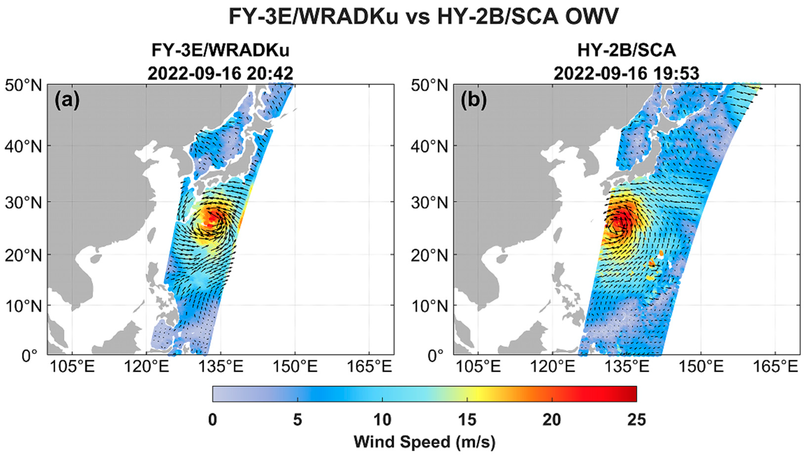
Figure 2.
Density scatter plot of collocated wind speeds between FY-3E/WRADKu and HY-2B/SCA for 2022. The plot includes the number of matched samples (N), mean bias, root mean square error (RMSE), Pearson correlation coefficient (R), and the least squares regression equation (red line). The dashed line represents the ideal 1:1 reference, and the color bar indicates point density (darker color indicates higher density).
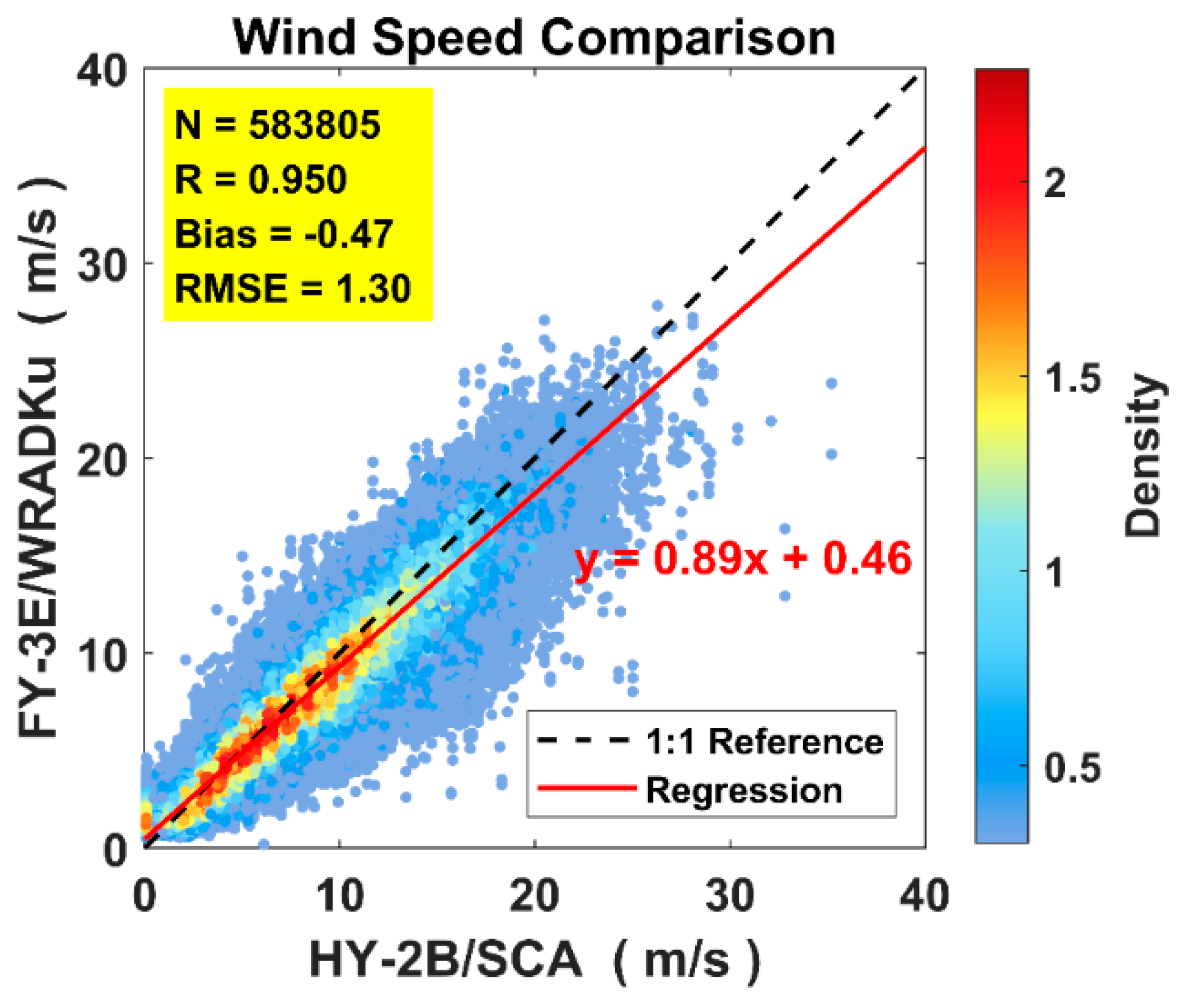
Figure 3.
Probability density distribution (PDF) of wind speed differences (FY-3E − HY-2B) for matched samples. Orange bars represent the normalized histogram, and the blue curve is the kernel density estimate. The distribution is sharply peaked with a heavier left tail, indicating a small number of large negative outliers.
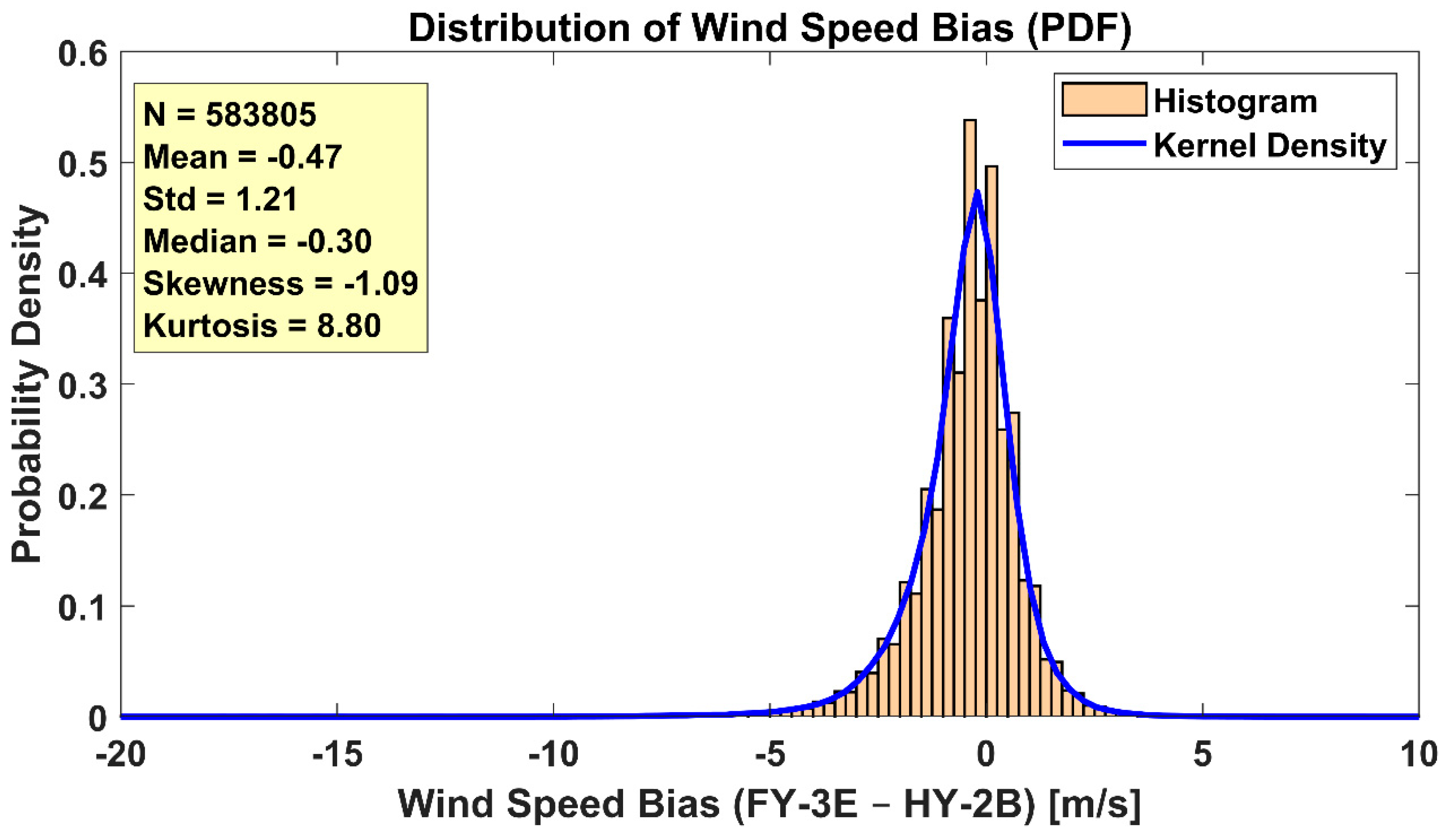
Figure 4.
Stratified statistics of wind speed differences between FY-3E/WRADKu and HY-2B/SCA in 2022 by Beaufort level. The left y-axis shows the mean bias ± 1σ; the right y-axis shows the number of matched samples per wind level. Dots represent statistical values for each category, annotated with sample counts. The x-axis indicates Beaufort scale levels (B0–B12), and the shaded box in the upper-right corner indicates the corresponding wind speed ranges for each level.
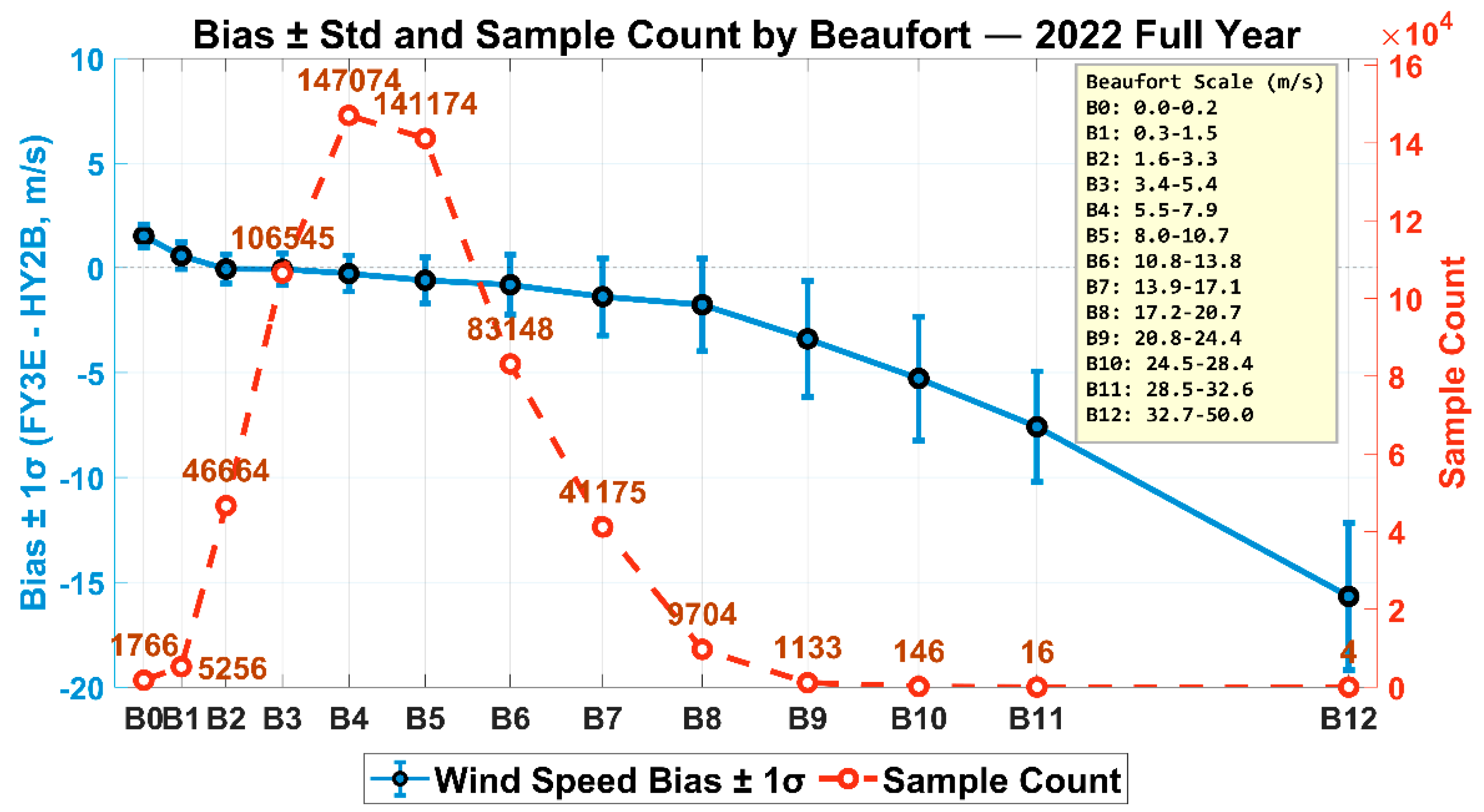
Figure 5.
Monthly intercomparison of wind speed products from FY-3E/WRADKu and HY-2B/SCA in 2022. Each subplot corresponds to a calendar month. The x-axis denotes Beaufort wind force levels (B0–B11). The left y-axis represents the mean wind speed bias of FY-3E relative to HY-2B/SCA with ±1σ error bars; the right y-axis shows the number of matched samples in each wind force category. The green solid line with error bars shows the bias statistics, while red dotted circles indicate sample counts. Most samples are concentrated in the B3–B6 range (3.4–13.8 m/s), with some increases in higher wind speed bins during summer and autumn months.
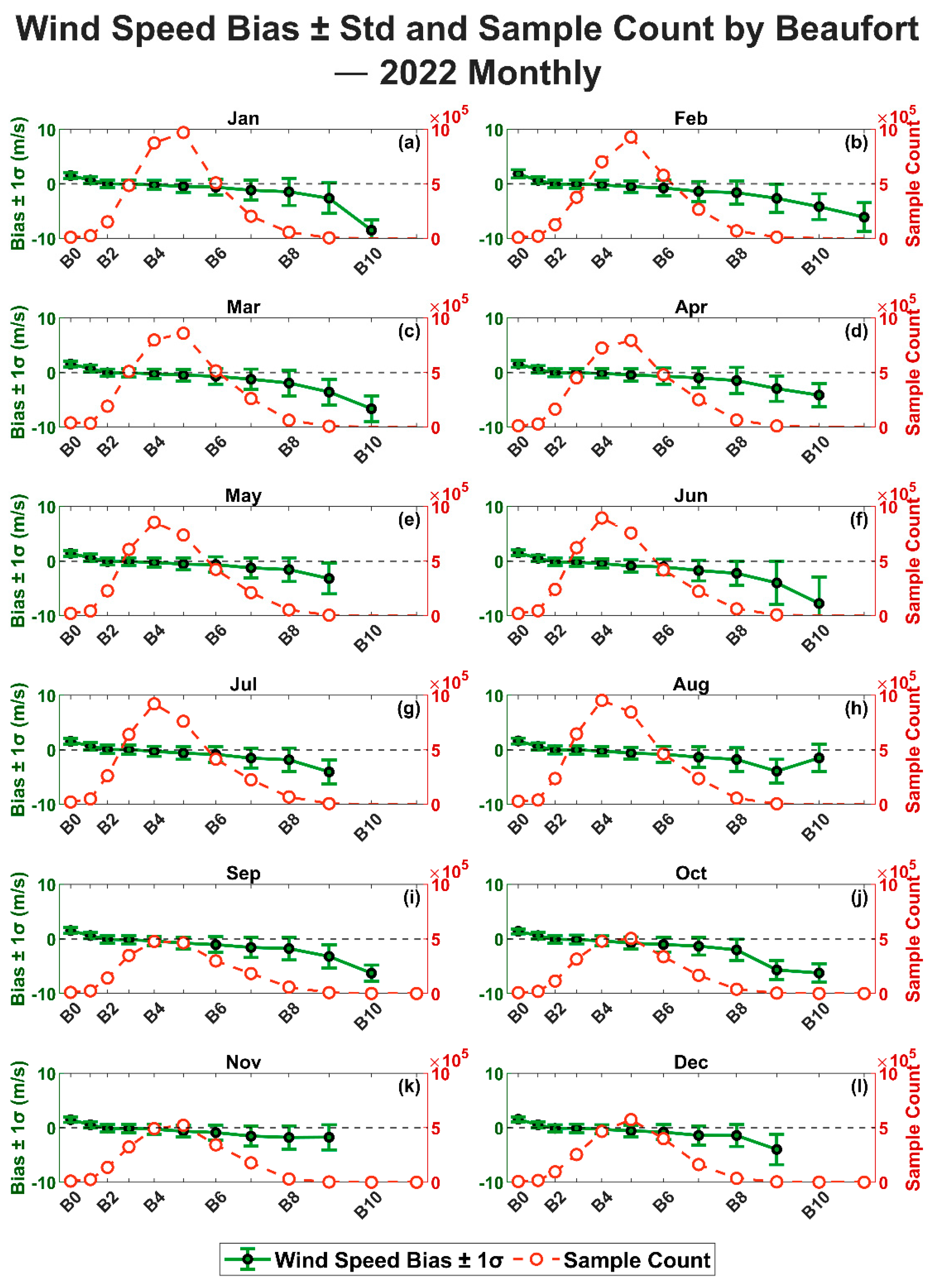
Figure 6.
Polar distribution of wind direction bias between FY-3E/WRADKu and HY-2B/SCA for the year 2022. The radial axis represents the number of collocated samples within each wind direction difference bin. The figure includes annotations for the circular mean bias and standard deviation (Mean Bias ± Std).
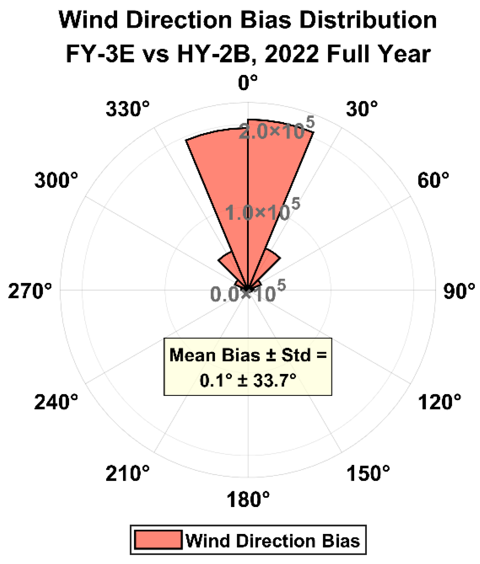
Figure 7.
Statistical results of wind direction bias between FY-3E/WRADKu and HY-2B/SCA in 2022 across different Beaufort wind force levels. The left y-axis shows the circular mean bias and its standard deviation (Bias ± 1σ, in degrees), while the right y-axis represents the number of matched samples in each category. The red solid line denotes the wind direction bias, and the blue dashed line indicates the sample count.
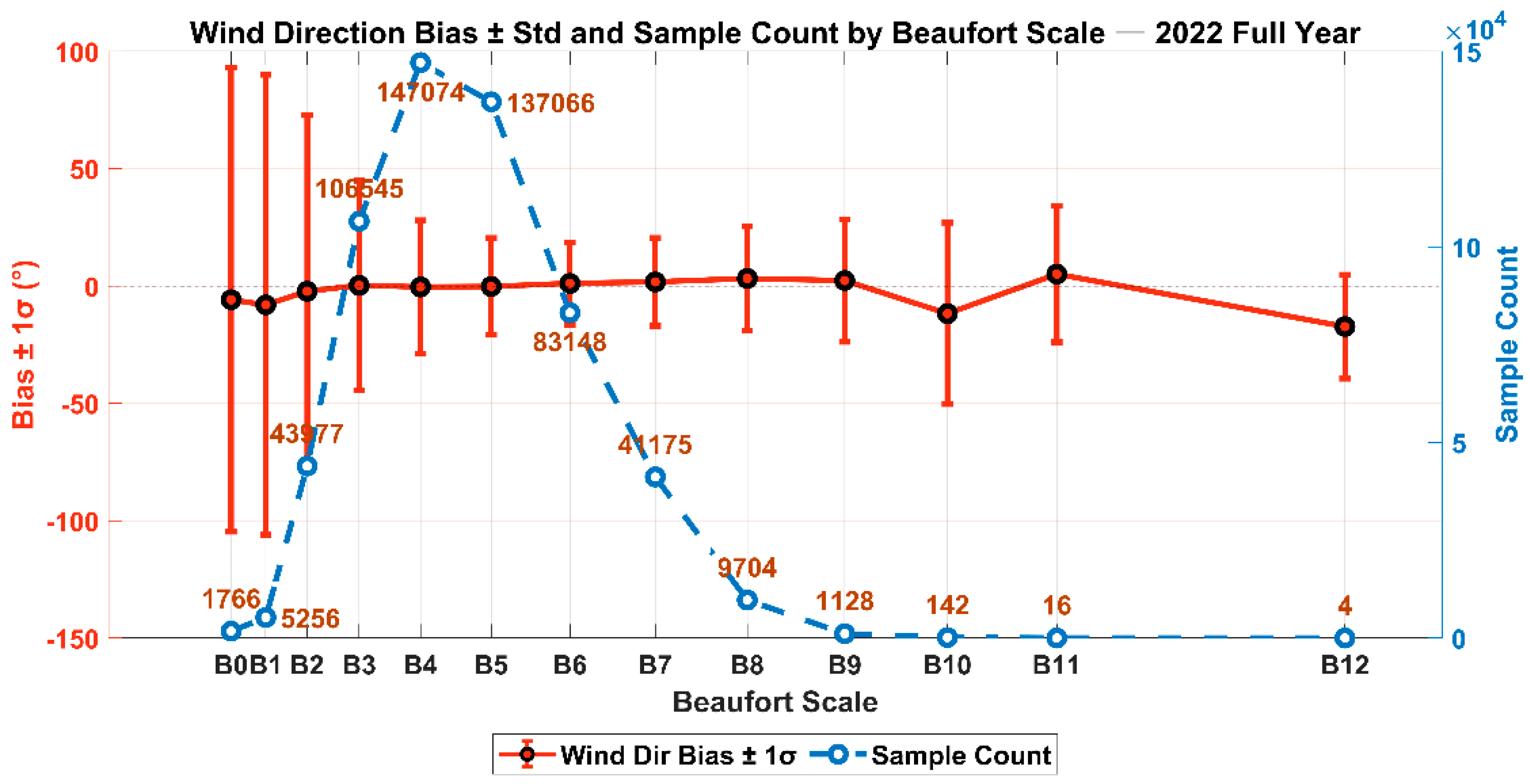
Figure 8.
Track and intensity evolution of Typhoon Hinnamnor (2022) from JTWC and China Meteorological Administration (CMA) best-track datasets. (a) Full best tracks from both agencies, with JTWC R34 (34-kt) quadrant wind radii overlaid at each analysis time. Line/marker colors denote intensity categories on the JTWC/CMA scales. (b) Close-up of the study period (UTC 2022-08-30 to 09-04) showing track points only. The four UTC analysis times used for scatterometer intercomparison—30 Aug 21:00, 31 Aug 21:00, 03 Sep 09:00, and 04 Sep 21:00—are highlighted and labeled. The legend distinguishes TD, TS, STS, TY; ST denotes Super Typhoon (JTWC label), while SuperTY denotes CMA category code 6 (Super Typhoon); EX indicates the extratropical stage and DB/LO denotes disturbance/low.
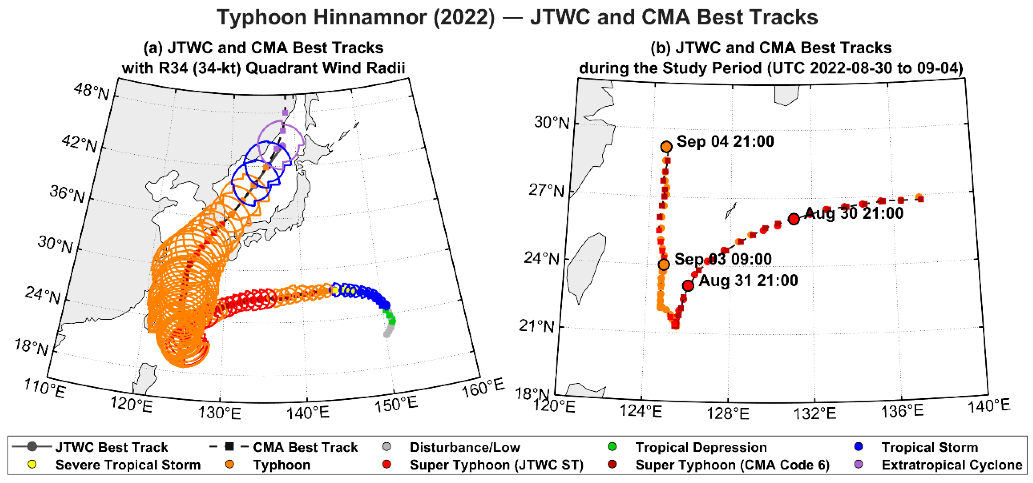
Figure 9.
Comparison of ocean surface wind fields from FY-3E/WRADKu, HY-2B/SCA, and the merged product during Typhoon Hinnamnor at four representative times. Panels (a, d, g, j) show FY-3E/WRADKu winds at (a) 21:04 UTC 30 August, (d) 21:10 UTC 31 August, (g) 21:10 UTC 3 September, and (j) 21:10 UTC 4 September 2022. Panels (b, e, h, k) show HY-2B/SCA winds at the corresponding times: (b) 20:30 UTC, (e) 21:02 UTC, (h) 20:27 UTC, and (k) 20:38 UTC. The time difference between the two satellites is indicated in the merged product panels. Panels (c, f, i, l) show the resulting merged wind product (displaying winds ≥ Beaufort scale 6) for each time step. In all panels, wind speed is represented by colors, wind direction by arrows. The green ‘x’ marks the typhoon center (JTWC). The purple and blue arcs represent the 34-knot wind radius (R34) derived from the merged product and JTWC, respectively.
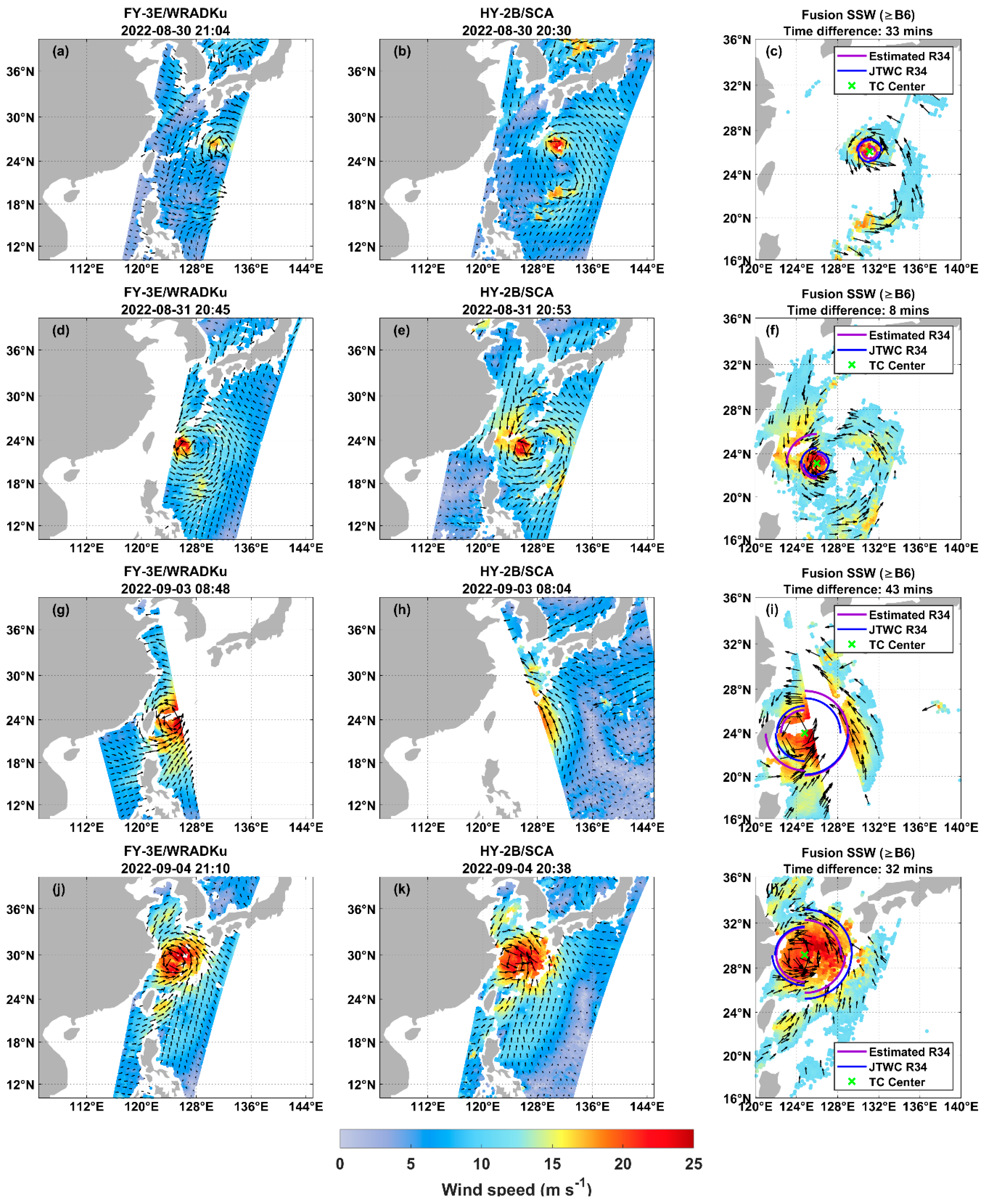
Figure 10.
Quantitative comparison of the 34-knot wind radius (R34) between the merged product and JTWC best track data during Typhoon Hinnamnor. (a-d) Temporal evolution of quadrant-specific R34 for the merged product (purple line) and JTWC (blue line) at (a) 2022-08-30 21:00 UTC, (b) 2022-08-31 21:00 UTC, (c) 2022-09-03 09:00 UTC, and (d) 2022-09-04 21:00 UTC. The Mean Diff value in each panel is the average difference across all four quadrants at that time. (e) Quadrant-wise differences (ΔR34 = Estimated - JTWC) for all four times. Colors represent different JTWC analysis times. The Mean Diff represents the overall average difference across all quadrants and times.
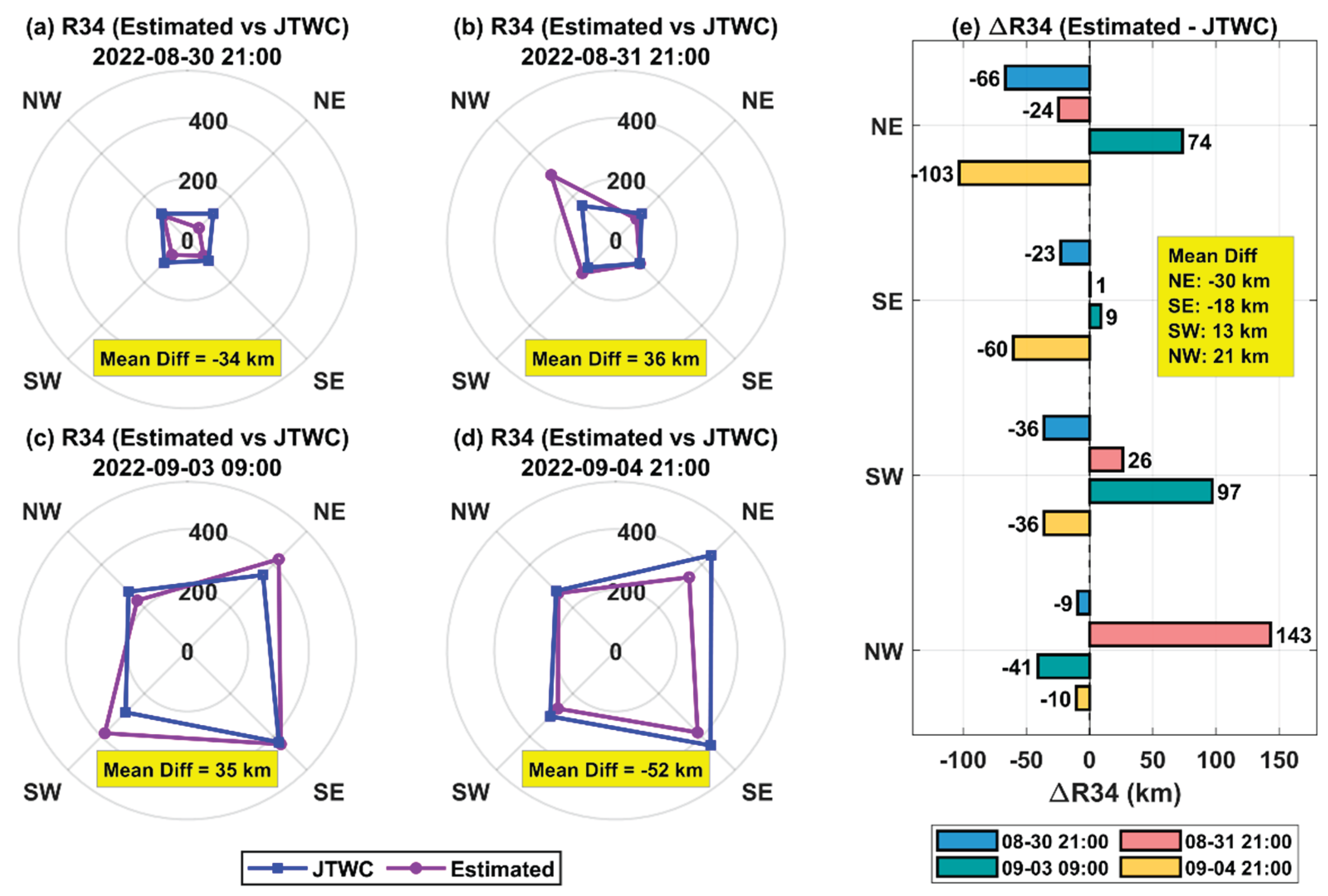

Table 1.
Technical specifications of FY-3E/WindRAD and HY-2B/SCA.
| Parameter | FY-3E/WindRAD | HY-2B/SCA |
| Orbit type | Sun-synchronous orbit | Sun-synchronous orbit |
| Equator crossing time | 05:30 (descending) / 17:30 (ascending) | 06:00 (descending) / 18:00 (ascending) |
| Orbital period | ~99 min per cycle | ~100 min per cycle |
| Global coverage cycle | Twice daily over global oceans | >90% coverage every 1–2 days |
| Wind measurement mode | Dual-frequency, dual-polarization, conical scanning scatterometer | Single-frequency, dual-polarization, conical scanning scatterometer |
| Operating frequency | C-band (5.3 GHz) + Ku-band (13.256 GHz) | Ku-band (13.256 GHz) |
| Polarization | HH, VV | HH, VV |
| Calibration | External calibration + onboard calibration | Onboard calibration |
| Spatial resolution | ~20–25 km | ~25 km |
| Swath width | ~1250–1300 km | 1350 km (H-pol), 1700 km (V-pol) |
| Observation cycle | Global coverage twice per day | Global coverage every 1–2 days |
| Wind retrieval model | CMOD7 (C-band), NSCAT-6 (Ku-band), CMOD7+NSCAT-6 (dual-frequency) | NSCAT-4 GMF model |
| Wind products | WRADC (C-band), WRADKu (Ku-band), WRADX (dual-frequency) | L2B wind speed and direction (HDF5) |
| Wind definition | 10 m stress-equivalent wind | 10 m stress-equivalent wind |
| Wind speed range | 3–40 m/s | 3–35 m/s |
| Quality control | Multi-bit QC flags (e.g., Bit13–Bit16) | Multi-bit QC flags (rain, land contamination, anomalies, retrieval failure) |
| Wind direction processing | MSS + 2DVAR ambiguity removal | MSS + 2DVAR ambiguity removal |
| Data format | HDF5 | HDF5 |
Note: MSS = Multiple Solution Sampling; 2DVAR = Two-Dimensional Variational method.
Table 2.
Beaufort scale classification for wind speed.
| Beaufort scale | Wind speed range (m/s) |
| 0 | <0.2 |
| 1 | 0.3–1.5 |
| 2 | 1.6–3.3 |
| 3 | 3.4–5.4 |
| 4 | 5.5–7.9 |
| 5 | 8.0–10.7 |
| 6 | 10.8–13.8 |
| 7 | 13.9–17.1 |
| 8 | 17.2–20.7 |
| 9 | 20.8–24.4 |
| 10 | 24.5–28.4 |
| 11 | 28.5–32.6 |
| 12 | ≥32.7 |
Disclaimer/Publisher’s Note: The statements, opinions and data contained in all publications are solely those of the individual author(s) and contributor(s) and not of MDPI and/or the editor(s). MDPI and/or the editor(s) disclaim responsibility for any injury to people or property resulting from any ideas, methods, instructions or products referred to in the content. |
© 2025 by the authors. Licensee MDPI, Basel, Switzerland. This article is an open access article distributed under the terms and conditions of the Creative Commons Attribution (CC BY) license (http://creativecommons.org/licenses/by/4.0/).
Copyright: This open access article is published under a Creative Commons CC BY 4.0 license, which permit the free download, distribution, and reuse, provided that the author and preprint are cited in any reuse.


