
Submitted:
16 October 2025
Posted:
17 October 2025
You are already at the latest version
Abstract
In this paper, we investigate the thread oscillation in a quiecent prominence observed by New Vacuum Solar Telescope at the Hα line center on 17 April 2024. Each individual thread is traced by the local maximum intensity on the time-distance maps. Although there are numerous threads in this prominence, 24 oscillating threads are identified at eight slits parallel to the solar surface. A sinusoidal function is used to fit them, and a mean period of 27.7 minutes is detected. We find that all these 24 threads display the oscillation with almost a constant amplitude, none damping or expansion during their lifetimes. Furthermore, we find the oscillations at different positions on a same thread are almost have similar period, the mean period is 87.7 min, which indicates that the threads are oscillating as a standing wave. Our finding would be the evidence of what mechanism drives the thread oscillations in quiecent prominence.
Keywords:
prominences
; thread oscillations
; quiescent
1. Introduction
Solar prominences/filaments are large-scale structures consisting of relatively cool and dense plasma embedded in the surrounding lower corona, which often lie above the magnetic polarity inversion lines [1]. Based on their location, they can be classified as active region (AR) or quiescent prominences/filaments. The latter has a long lifetime of tens days or more. The AR prominences/filaments tend to be more dynamic and short-lived, usually accompany the solar flares or coronal mass ejection (CME) in many studies [2–7]. Observationally, prominences/filaments have two linked categories of structures, such as spines and barbs [8–11]. The spine is the horizontal axis of the prominence/filament, while the barb connects the high spine and terminate in the chromosphere.
Different from the filaments located on the solar disk, the prominences are commonly observed as elongated features of a loop or arc shapes on solar limb [12,13]. The quiescent prominences stay in an equilibrium of the balance between the upward magnetic hoop force and the downward magnetic tension of the overlying coronal magnetic field, which is thought to be the spine. Different from the AR prominences, the quiescent prominences are usually observed in the polar crown regions at high latitudes (). High resolution observations have resolved numerous thin threads in the prominences and they display highly dynamics [14–18]. One of the most attractive behaviors is the oscillations. Using the Hinode/SOT observations, we found that two spines of a prominence exhibits the oscillations with a period of 9.8 min [11]. Meanwhile, we also found that the threads in this prominence display the oscillation with a dominant period of 5 min [19]. Recently, the prominence threads are found to show the oscillation at a period of 26 min, and some of them display their intensity oscillations with a mean period of 8 min simultaneously [20]. Actually, numerous studies have analyzed the thread oscillations in the prominences [20–29]. This is because the prominences display lots of vertical threads on the limb, and such threads are thought to be the vertical magnetic field lines [16,30–34]. The oscillations are proposed to the evidences of Alfven waves propagating in the prominence threads [17,30]. However, the magnetohydrodynamics (MHD) stimulations show that the vertical threads in the prominence are caused by the magnetic Rayleigh-Taylor instability process [35]. Therefore, the nature of the oscillations of the vertical threads in the prominence is still an open issue.
2. Observation and Data Analysis
NVST is a vacuum solar telescope with 985 mm clear aperture located at Fuxian Lake in China at an approximate altitude of 1700 m. It has an imaging system, an adaptive optic system [37], and a spectrometer for now. The imaging system has two channels, such as H and TiO-band. The H channel is equipped with a tunable Lyot filter with a bandwidth of 0.25 Å, which can record the image in the Å range with a step size of 0.1 Å. In this paper, we studied the quiescent prominence detected by NVST in the H center (6562.8 Å). The field of view (FOV) of these H images is , with a 12 s cadence and a CCD plate scale of 0.165”/pixel [36].
The prominence studied here was located at the solar northwest limb, with a coordinate of N02W59. It was observed by NVST from 02:40 to 05:05 UT on April 17 2024. Figure 1 shows the H center image of the prominence at 04:06:09 UT. All of the NVST H images are normalized by the quiet Sun, and to eliminate the effect of seeing and aligned with each other based on a cross-correlation algorithm [38]. This prominence is observed with a perpendicular direction to its spine, which has a cross-section of about 360 Mm2. There are numerous threads almost perpendicular to the solar surface. One end of the most threads is rooted into the solar photosphere, but the other end is suspended into the chromosphere towards the corona. Continuous observations such as the data movie show that these threads are not stationary but highly dynamic and display the oscillations parallel to the solar surface. A bubble is seen in the middle of the prominence ranging from 55 Mm to 65 Mm at the y-axis.
Figure 2 plots the time-distance maps of H intensity along eight slits. The length of slits is about 450 pixels (60 Mm), and the distance between two adjacent slit is same as 15 pixels (2 Mm), which is larger than the thread width, i.e., 1.2 Mm [14,19,39]. The H intensity is integrated by a width of 8 pixels around each slit. The bright regions represent H prominence, while the dark regions indicate the corona on the boundaries of prominence. Figure 2 shows that these threads are dynamic. Some threads display the drifting motions, but some exhibit oscillation motions, and even some are stable during the observational interval. Thus, it is possible that the threads intersect with each other at certain times. For example, the regions from 15 to 25 Mm along y-axis and between 04:10 UT and 04:25 UT at slit of S1; from 10 to 25 Mm and between 03:00 UT and 03:40 UT along slit of S3 in Figure 2 could be several threads overlapping together. Not all but only the threads exhibiting oscillations are studied in this paper.
In order to investigate thread oscillations in prominence, we have to trace the thread location at each time. Observationally, the continuous bright lines in the time-distance maps are thought to be the individual thread. Figure 2 shows that there are a lot of the continuous bright lines. However, most of them are fragmented with a short lifetime, which results into being hard to detect the oscillating motions. Actually, Figure 2 shows that there are some threads exhibiting the oscillations. Some of them are oscillating started at the NVST observation, i.e., at 02:40 UT, and some threads are oscillating in the middle of the observational interval. Firstly, we use naked-eyes to search for the threads displaying oscillations, and then determine the starting point with the local maximum intensity. For example, we judge an oscillating thread along the y-axis from 48 to 51 Mm at 02:40 UT in the time-distance map of S1. It is marked by Thread-1 in Figure 2. The first point is detected at 50 Mm with the local maximum intensity. The second point in the next time could be near 50 Mm, which has a location of 379 pixel along y-axis. Therefore, the second point is identified from the seven points around the center point of 379 pixel at the next cadance, such as 376, 377, 378, 379, 380, 381, 382 pixels along y-axis pixel, with the maximum intensity among them. We find that the second point is located at 380 pixels along y-axis. Then the 380 pixel is the center point of the third point which has a local maximum intensity among seven points around it. We use this method to find the subsequent points on the thread. It is possible that there are two or more points with the local maximum intensity. The point with the shortest distance from the center point is identified as the thread. At a time, if the point has a local maximum intensity less than the noise level, i.e., three times standard deviation plus the mean value at the background, or the several threads cross each other at this point, the thread is identified to stop here. For example, Thread-1 is stopped at 03:09 UT due to other threads overlapped, while Thread-5 is stopped at 03:42 UT due to the weak brightness less than noise level. In total, 24 individual oscillating threads are identified in the eight time-distance maps in Figure 2. Each thread is traced by the blue dots, and they all display the oscillating behaviors. Actually, none of oscillating threads is detected in the time-distance map at S8. Although there are many threads, either drifting motion or crossed each other with a short lifetime. Slit of S8 is located in the top of prominence, which is highly dynamic resulting in the thread fragmentation.
After detecting the oscillating threads, we use the following function to fit:
where A represents the amplitude, P represents the oscillating period, b represents the drifting speed of the thread. The blue solid lines are fitting results shown in Figure 2.
Figures 3–5 show the fitting of 24 threads in detail. For each thread, for example, Thread-1 in Figure 3, top panel plots the time-distance map of H intensity with a small window from 02:40 UT to 03:12 UT in its lifetime. The blue dots trace the location fluctuation on the thread. The green line represents the function fitting. Second panel plots the thread with the blue dots and the drifting motion with the orange line. Thread-1 has a drifting speed of 0.65 km/s. Third panel shows the oscillating behavior of Thread-1 removing the drifting component. A complete oscillation is found in Thread-1 as the sinusiodual function with a period of 16 min. For the Thread-2, it has a drifting speed of 0.35 km/s, but the drifting direction is inverse from the Thread-1. Namely, Thread-1 and Thread-2 are drifting parallel to the solar surface, but with opposite directions. In this paper, the thread drifting speeds are estimated but ignored the directions.
Figure 3.
Zoom out the Thread-1 to Thread-8 to show the function fitting in detail. For each thread, the blue dots trace the threads with the local maximum intensity, and the green lines represent the function (1) fitting (top). Orange line is the drifting motion of the threads (middle). Each bottom, the blue dots are thread behavior removing the drifting motion and the green lines shows the sinusiodal fitting.
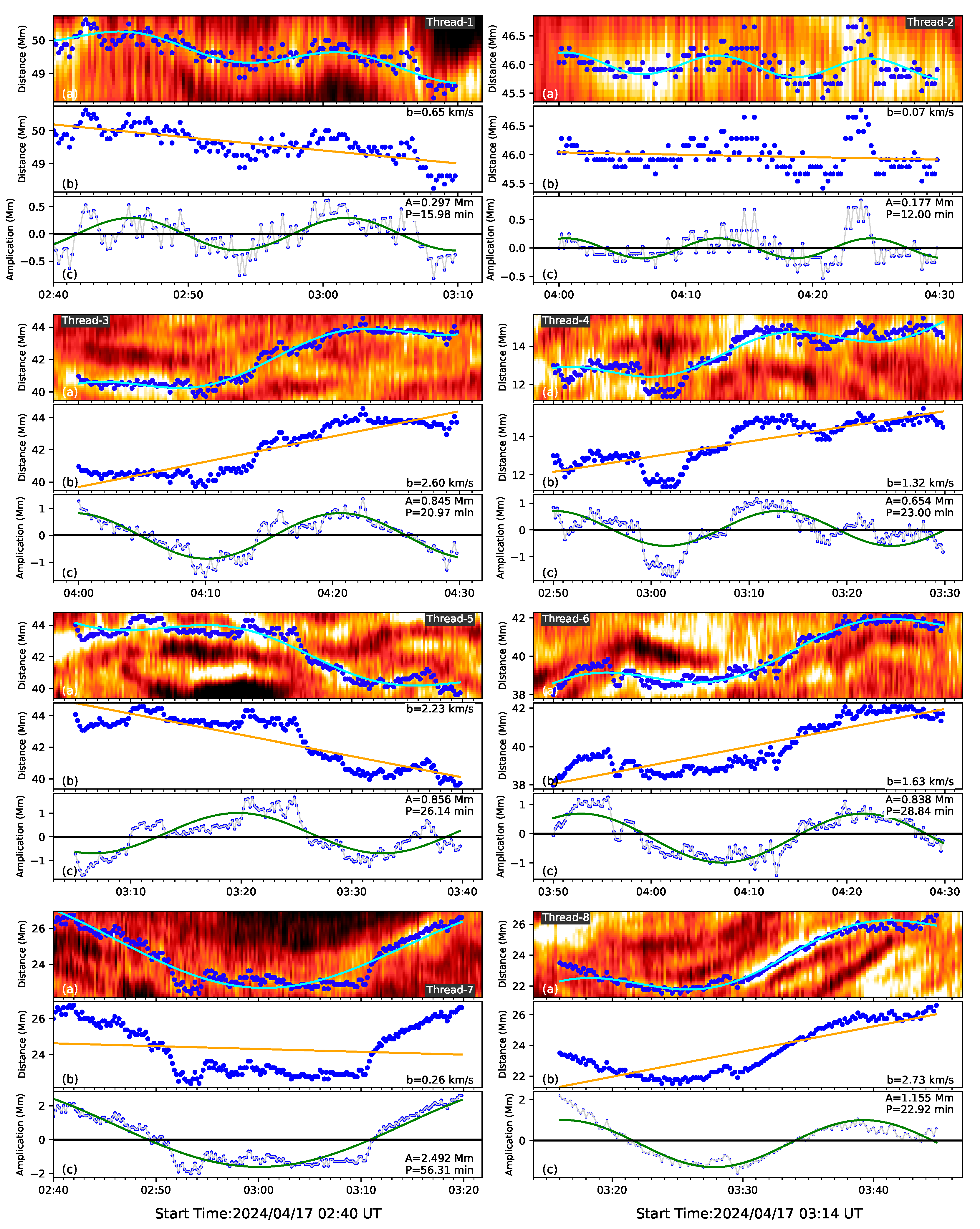
Figure 4.
Same as Figure 3, but for the Thread-9 to Thread-16.
Figure 4.
Same as Figure 3, but for the Thread-9 to Thread-16.
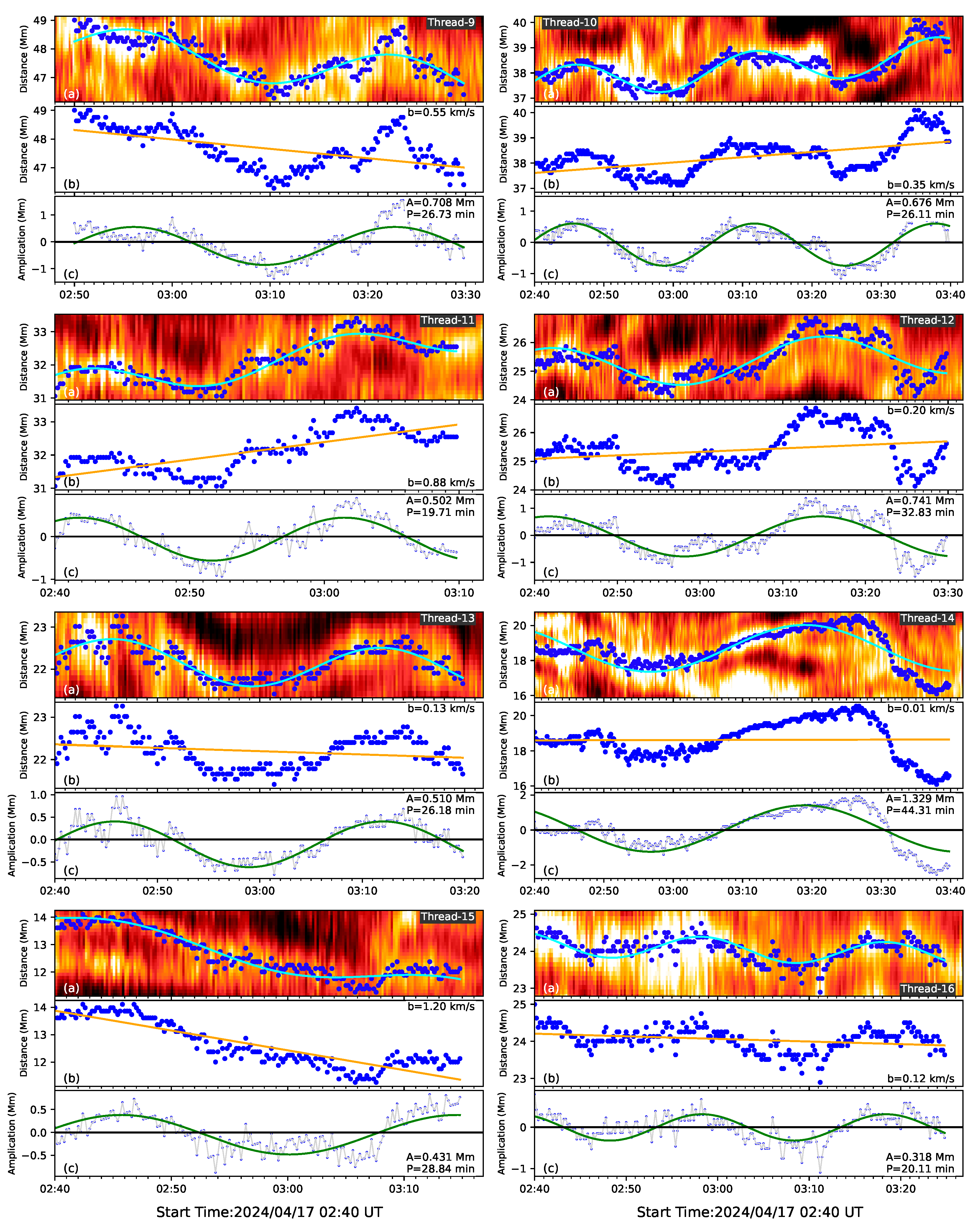
Figure 5.
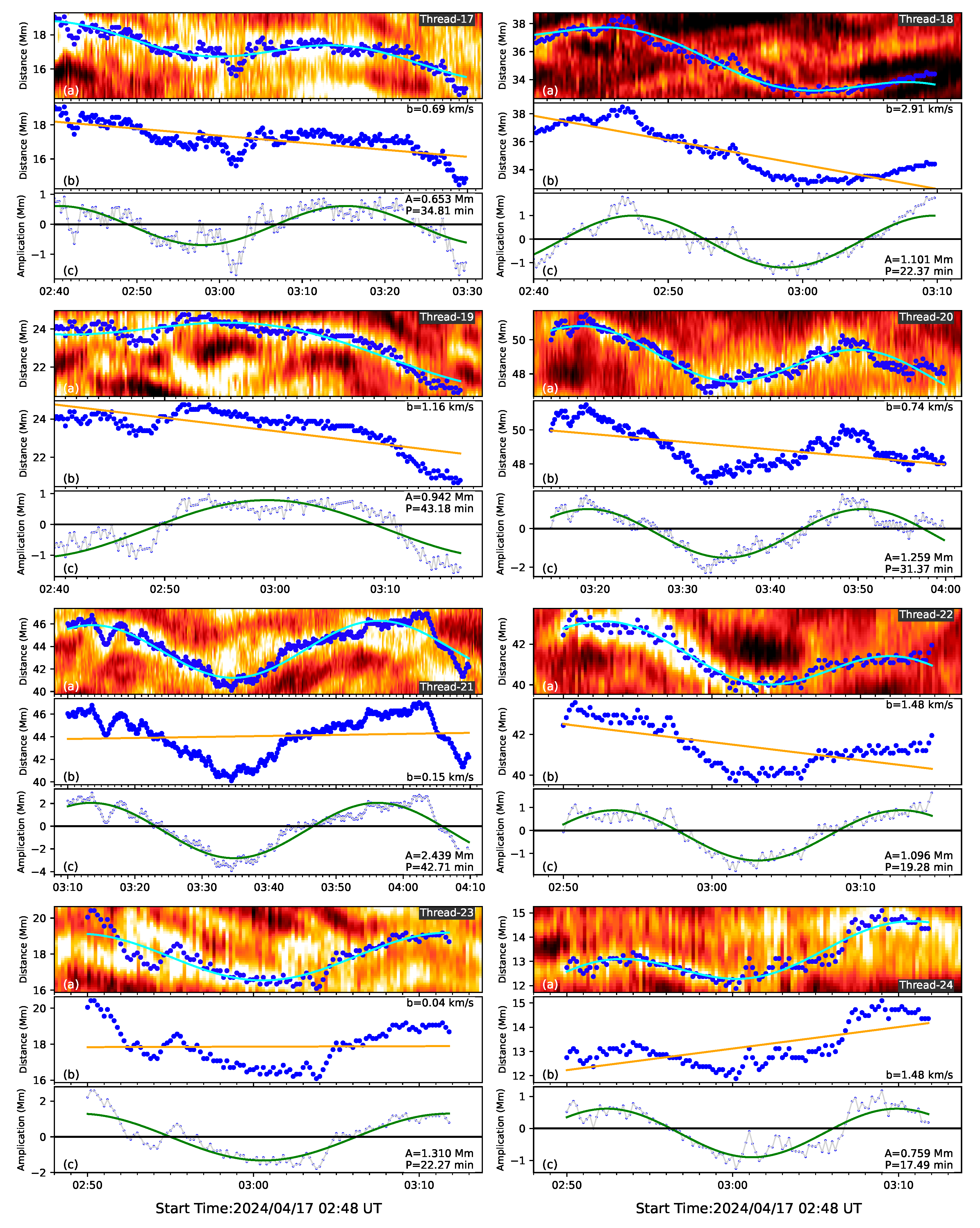
Same as Figure 3, but for the Thread-17 to Thread-24.
Figure 5.
Same as Figure 3, but for the Thread-17 to Thread-24.
3. Results
Using the function (1) to fit 24 oscillating threads, the parameters such as the period of P, the amplitude of A and the drifting speed of b, cycles of oscillations and lifetime of oscillations are listed in Table 1. We find the oscillating periods between 12 minutes and 43.18 min. The amplitude between 0.18 Mm and 2.49 Mm. The drifting speed between 0.04 km/s and 2.91 km/s. The oscillating thread lifetime between 22 min and 60 min. We find most of threads could display a complete cycle of oscillation here. The cycle of thread oscillation is detected by the oscillating lifetime divided by period. Thread-2 displays two and half cycles of oscillations with the shortest period of 12 min and the smallest drifting speed of 0.07 km/s among 24 threads. Thread-19 has the longest period of 43.18 min. The largest drifting speed of 2.91 km/s is detected in Thread-18. Thread-13 and Thread-21 have a longest oscillating lifetime of 60 min but with one and almost half cycle of oscillations. We find that each thread shows its oscillation with a constant amplitude, no damping and no expansion.

Table 1.
The parameters of the displacement oscillation detected in 24 threads.
| Thread | P(min) | A(Mm) | b(km/s) | Cycles of Oscillation | Lifetime of Ocsillation(min) |
|---|---|---|---|---|---|
| Thread-1 | 15.98 | 0.30 | 0.65 | 1.88 | 30 |
| Thread-2 | 12.00 | 0.18 | 0.07 | 2.50 | 30 |
| Thread-3 | 20.97 | 0.85 | 2.60 | 1.43 | 30 |
| Thread-4 | 23.00 | 0.65 | 1.32 | 1.74 | 40 |
| Thread-5 | 26.14 | 0.86 | 2.23 | 1.34 | 35 |
| Thread-6 | 28.84 | 0.84 | 1.63 | 1.39 | 40 |
| Thread-7 | 56.31 | 2.49 | 0.26 | 0.71 | 40 |
| Thread-8 | 22.92 | 1.16 | 2.73 | 1.27 | 29 |
| Thread-9 | 26.73 | 0.71 | 0.55 | 1.50 | 40 |
| Thread-10 | 26.11 | 0.68 | 0.35 | 2.30 | 60 |
| Thread-11 | 19.71 | 0.50 | 0.88 | 1.52 | 30 |
| Thread-12 | 32.83 | 0.74 | 0.20 | 1.52 | 50 |
| Thread-13 | 26.18 | 0.51 | 0.13 | 1.53 | 40 |
| Thread-14 | 44.31 | 1.33 | 0.01 | 1.35 | 60 |
| Thread-15 | 28.84 | 0.43 | 1.20 | 1.21 | 35 |
| Thread-16 | 20.12 | 0.32 | 0.12 | 2.24 | 45 |
| Thread-17 | 34.81 | 0.65 | 0.69 | 1.44 | 50 |
| Thread-18 | 22.37 | 1.10 | 2.91 | 1.34 | 30 |
| Thread-19 | 43.18 | 0.94 | 1.16 | 0.86 | 37 |
| Thread-20 | 31.37 | 1.26 | 0.74 | 1.43 | 45 |
| Thread-21 | 42.71 | 2.44 | 0.15 | 1.40 | 60 |
| Thread-22 | 19.28 | 1.10 | 1.48 | 1.30 | 25 |
| Thread-23 | 22.28 | 1.31 | 0.04 | 0.99 | 22 |
| Thread-24 | 17.49 | 0.76 | 1.48 | 1.26 | 22 |
Figure 6 plots the histograms of the fitting parameters, including the periods (a), amplitudes (b), drifting speeds (c), cycles (d) and the lifetime (e) of oscillations, and the mean values of these parameters are given. About 79 % (19/24) threads have an oscillating period between 15 minutes and 35 min, 75 % (18/24) threads have an oscillating amplitude between 0.5 Mm and 1.5 Mm. 58 % (14/24) threads have a small drifting speed less than 1 km/s. Here, the speed direction can be ignored. These threads have a mean period of 27.7 min, mean amplitude of 0.92 Mm, mean drifting speed of 1.0 km/s, mean cycle of 1.5 and mean oscillating lifetime of 38.5 min. Most of threads, 87 % (21/24) display one cycle in our observation interval.
4. Discussions and Conclusions
In this paper, we studied the thread oscillations in a quiescent prominence observed by NVST at H line center on 17 April 2024. High resolution observations show the numerous threads in this prominence, which has a cross-section about . Eight slits with a distance of 2 Mm are set to plot the time-distance maps, on which the threads exhibit highly dynamics, such as drifting motion and oscillations. Based on our data, we develop a method to trace the local maximum intensity to identify each individual thread. Although this prominence has a lot of threads, we just detect the oscillating threads, which almost display one whole cycle of oscillation in this paper. The threads are ruled out to study here because they can not be detected obvious oscillation during their lifetime. Although three threads such as the threads of 7, 19, 13 do not display a whole cycle of oscillation during their lifetime, they do have an obvious oscillation behavior, about 0.7 cycle of oscillation period at least. In total, 24 threads are identified to exhibit the oscillations. Using a sinuoudal function to fit their behavior, we statistically study the parameters such as the period, amplitude, drifting speed, cycle and the lifetime of oscillations. And we also find the mean period of 27.7 min, mean amplitude of 0.82 Mm, mean drifting speed of 1.0 km/s. The Thread-2 has a shortest period of 12 min and displays two and half cycles of oscillating in its 30 min lifetime. Most of threads exhibit oscillation cycles about 1.3.
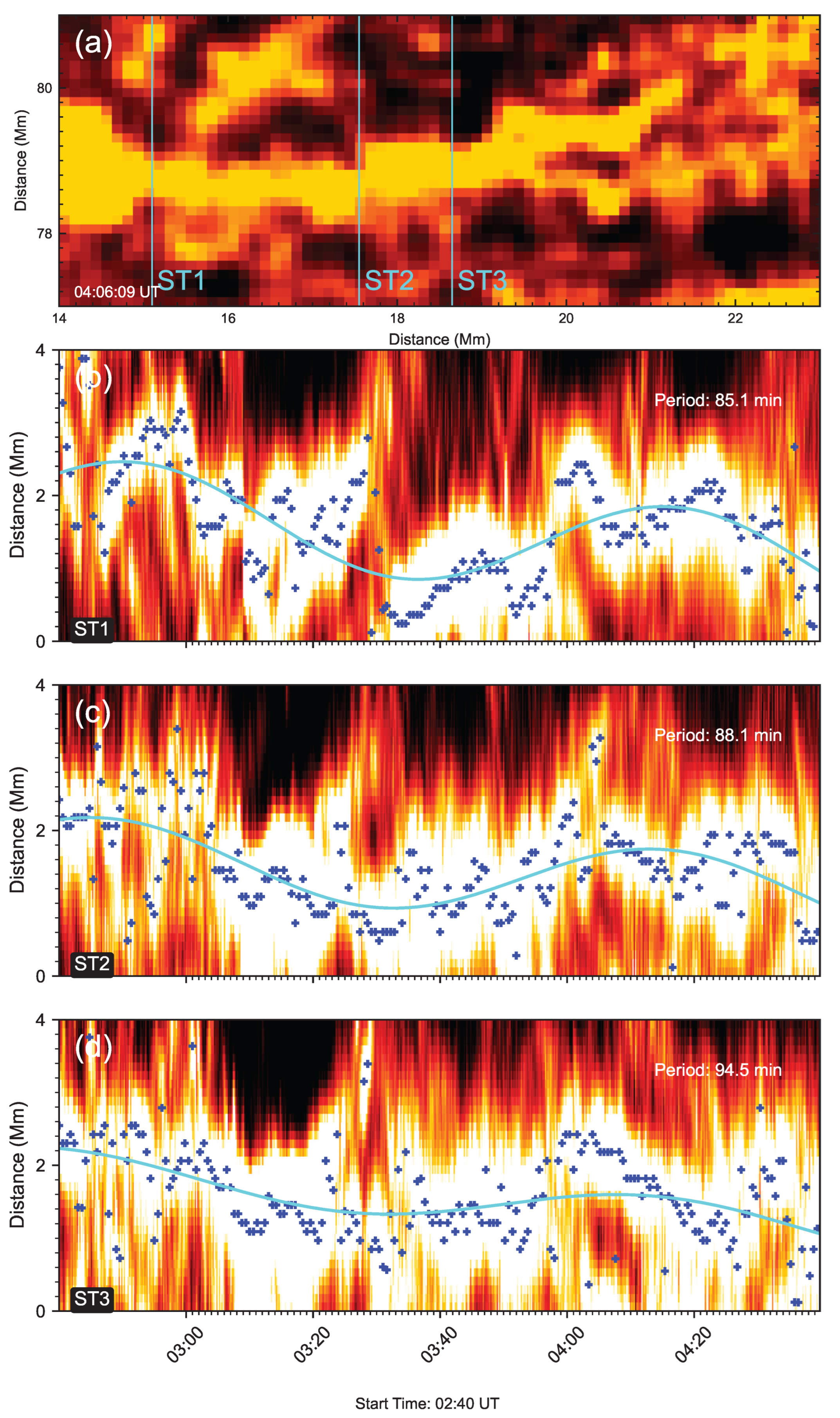
Generally, the vertical threads of prominences are thought to be the cool condensed plasma filled into the vertical magnetic flux tube. The thread oscillating parallel to the solar surface that we found here could indicate that the MHD waves propagating from the photosphere to the chromosphere and corona [20,30,35,40]. Such MHD waves are either propagating or standing waves. In order to investigate which mode of waves works in our observation, the oscillations at various positions along a same thread (a cyan box in Figure 1) is analysed in detail. Figure 6 (a) plots the H image of this thread at 04:06:09 UT. It has a length of 8 Mm. There are slits of ST1, ST2 and ST3 are located in the different position, the position of each slit is selected randomly and the distance between each slit is not the same. Figure 6 (b, c, d) show the time-distance maps in it lifetime from 02:40 UT to 04:30 UT. Using the same method, the thread is traced by the local maximum intensity using the blue dots and fitted them with the function (1) as the green lines. The results show that the oscillations at these positions are almost in the same phase, which suggests that the thread oscillation is very likely to be a standing wave. It is still an open issue which mechanism triggers the MHD waves. Meanwhile, we do not find the amplitudes of thread oscillations changes with height. In other words, these standing waves are almost stable from the photosphere to chromosphere, suggesting no energy diffusion in the atmosphere. On the other hand, we do not identify a thread to exhibit one whole cycle of oscillation on the top of the prominence, i.e., in the time-distance map at slit of S8, in which many threads are there, but only displaying the drifting motions. It is possible that the threads on the top of the prominence are fragmental due to the plasma turbulence there. Another possibility is that the threads display their oscillations are not parallel but oblique to the solar surface. Therefore, the thread oscillations in the prominence need more studies in the future.
Figure 7.
Oscillations at three positions of the thread encycled by the cyan box in Figure 1 (a), H image of the thread at 04:06:09 UT (b)-(c), time-distance maps corrospanding the these perpendicular slits marked by ST1, ST2, ST3 in (a).
Figure 7.
Oscillations at three positions of the thread encycled by the cyan box in Figure 1 (a), H image of the thread at 04:06:09 UT (b)-(c), time-distance maps corrospanding the these perpendicular slits marked by ST1, ST2, ST3 in (a).
Acknowledgments
This work is supported by the Strategic Priority Research Program of the Chinese Academy of Sciences grant No. XDB0560000, the National Key R&D Program of China 2022YFF0503002 (2022YFF0503000), and the NSFC under grants 12073081 and 12250014.
References
- Martin, S. F. Conditions for the formation and maintenance of filaments. Sol. Phys. 1998, 182, 107–137. [Google Scholar] [CrossRef]
- Pooja, A., et al. Dynamics of active region filaments associated with flares and CMEs. Astrophys. J. 2025, (to be published).
- Zhuang, B., et al. Magnetic structure of eruptive prominences. Astron. Astrophys. 2025, (to be published).
- Gopalswamy, N.; Lara, A.; Yashiro, S.; Howard, R. A. Coronal mass ejections and associated prominence eruptions. Astrophys. J. 2003, 586, 562–578. [Google Scholar] [CrossRef]
- Gilbert, H. R.; Holzer, T. E.; Burkepile, J. T.; Hundhausen, A. J. Dynamics of prominence threads. Astrophys. J. 2000, 537, 503–515. [Google Scholar] [CrossRef]
- Hori, K. Prominence oscillations and their implications. Publ. Astron. Soc. Japan 2002, 54, 287–296. [Google Scholar]
- Vršnak, B.; Ruždjak, V.; Brajša, R.; Džubur, A. Observational study of quiescent prominences. Sol. Phys. 1994, 152, 211–225. [Google Scholar]
- Engvold, O. Structure and dynamics of solar prominences. Sol. Phys. 1998, 182, 35–48. [Google Scholar]
- Zirker, J. B.; Engvold, O.; Martin, S. F. Magnetic topology of prominence spines and barbs. Nature 1998, 396, 440–441. [Google Scholar] [CrossRef]
- Zong, W. G.; Tang, Y. H.; Fang, C. High-resolution observations of prominence threads. Astron. Astrophys. 2003, 412, 267–274. [Google Scholar] [CrossRef]
- Ning, Z.; Cao, W.; Okamoto, T. J.; Ichimoto, K.; Qu, Z. Q. Oscillations in a solar prominence observed by Hinode. Astrophys. J. 2009, 699, 15–22. [Google Scholar] [CrossRef]
- Gibson, S. E.; Fan, Y. Prominence formation by magnetic condensation. Astrophys. J. 2006, 637, L65–L68. [Google Scholar] [CrossRef]
- Parenti, S. Solar prominences: Observations. Living Rev. Sol. Phys. 2014, 11, 1. [Google Scholar] [CrossRef]
- Lin, Y.; Engvold, O.; Wiik, J. E. High-resolution observations of prominence dynamics. Sol. Phys. 2003, 216, 109–120. [Google Scholar] [CrossRef]
- Lin, Y.; Engvold, O.; Rouppe van der Voort, L. Thin threads in solar prominences. Sol. Phys. 2005, 226, 239–250. [Google Scholar] [CrossRef]
- Chae, J.; Ahn, K.; Lim, E.-K.; et al. Dynamics of prominence threads from ground-based observations. Astrophys. J. 2008, 689, L73–L76. [Google Scholar] [CrossRef]
- Berger, T. E.; Shine, R. A.; Slater, G. L.; et al. Hinode/SOT observations of quiescent prominence oscillations. Astrophys. J. 2008, 676, L89–L92. [Google Scholar] [CrossRef]
- Xue, Z. K.; Yan, X. L.; Yang, L. H.; et al. High-resolution observation of prominence threads with NVST. Res. Astron. Astrophys. 2021, 21, 123. [Google Scholar] [CrossRef]
- Ning, Z.; Cao, W.; Goode, P. R. Five-minute oscillations in prominence threads. Astron. Astrophys. 2009, 499, 595–600. [Google Scholar] [CrossRef]
- Song, Y.; et al. Oscillation properties of prominence threads. Astrophys. J. 2024, (to be published).
- Shen, Y.; Liu, Y.; Liu, Y. D. Observations of a filament eruption and associated wave. Astrophys. J. 2014, 786, 151. [Google Scholar] [CrossRef]
- Shen, Y.; et al. Kink oscillations in coronal loops. Astrophys. J. 2017, 851, 67. [Google Scholar] [CrossRef]
- Zhang, Q. M.; et al. Prominence thread oscillations from high-resolution observations. Mon. Not. R. Astron. Soc. 2024, 533, 1234–1245. [Google Scholar]
- Zhang, Q. M.; et al. Longitudinal oscillations in a solar prominence. Astron. Astrophys. 2012, 542, A52. [Google Scholar] [CrossRef]
- Tripathi, D.; et al. Prominence seismology using MHD waves. Space Sci. Rev. 2009, 149, 283–298. [Google Scholar] [CrossRef]
- Luna, M.; et al. Prominence oscillations driven by external perturbations. Astrophys. J. Suppl. Ser. 2018, 236, 35. [Google Scholar] [CrossRef]
- Hersow, A.; et al. Magnetic field structure in oscillating prominences. Astron. Astrophys. 2011, 531, A45. [Google Scholar]
- Takahashi, T.; et al. Multi-wavelength observations of prominence oscillations. Astrophys. J. 2015, 807, 37. [Google Scholar] [CrossRef]
- Tripathi, D.; et al. Prominence dynamics and oscillations. Astron. Astrophys. 2006, 449, 369–378. [Google Scholar] [CrossRef]
- Okamoto, T. J.; Tsuneta, S.; Berger, T. E.; et al. Alfvén waves in prominence threads. Science 2007, 318, 1577–1580. [Google Scholar] [CrossRef]
- Oya, Y.; et al. Magnetic field structure in solar prominences. Publ. Astron. Soc. Japan 2008, 60, S7. [Google Scholar]
- Chae, J. The magnetic field of prominence threads. Astrophys. J. 2010, 714, 618–627. [Google Scholar] [CrossRef]
- Dudík, J.; Aulanier, G.; Schmieder, B.; et al. Magnetic topology of prominences. Astrophys. J. 2012, 761, 9. [Google Scholar] [CrossRef]
- Schmieder, B.; Chandra, R.; Berlicki, A.; et al. Velocity and magnetic field in a prominence. Astron. Astrophys. 2010, 514, A68. [Google Scholar] [CrossRef]
- Jenkins, J. M.; Keppens, R. Magnetic Rayleigh–Taylor instability in prominences. Astron. Astrophys. 2022, 663, A12. [Google Scholar]
- Liu, Z.; Xu, J.; Gu, B. Z.; et al. The New Vacuum Solar Telescope: Instrumentation and first results. Res. Astron. Astrophys. 2014, 14, 705–718. [Google Scholar] [CrossRef]
- Zhong, Y.; et al. Adaptive optics system of the New Vacuum Solar Telescope. Res. Astron. Astrophys. 2023, 23, 045. [Google Scholar]
- Yang, Y. Z.; Ji, K. F.; Feng, S.; et al. Image alignment method for high-resolution solar observations. Sol. Phys. 2015, 290, 2463–2475. [Google Scholar]
- Lin, Y. Prominence fine structures and their dynamics. Space Sci. Rev. 2011, 158, 237–258. [Google Scholar] [CrossRef]
- Wang, T.; Ofman, L.; Davila, J. M.; Su, Y. Growing transverse oscillations of a multistranded loop observed by SDO/AIA. Astrophys. J. Lett. 2012, 751, L27. [Google Scholar] [CrossRef]
Figure 1.
NVST H image of the quicent prominence on April 17 2024 at 04:06:09 UT. The scale in the Figure indicates the actual distance in megameters (Mm). The blue dashed lines represent the eight slits marked by S1, S2, S3, S4, S5, S6, S7, S8 to plot the time-distance maps in Figure 2.The distance between two slit is 2 Mm (about 16 pixels).
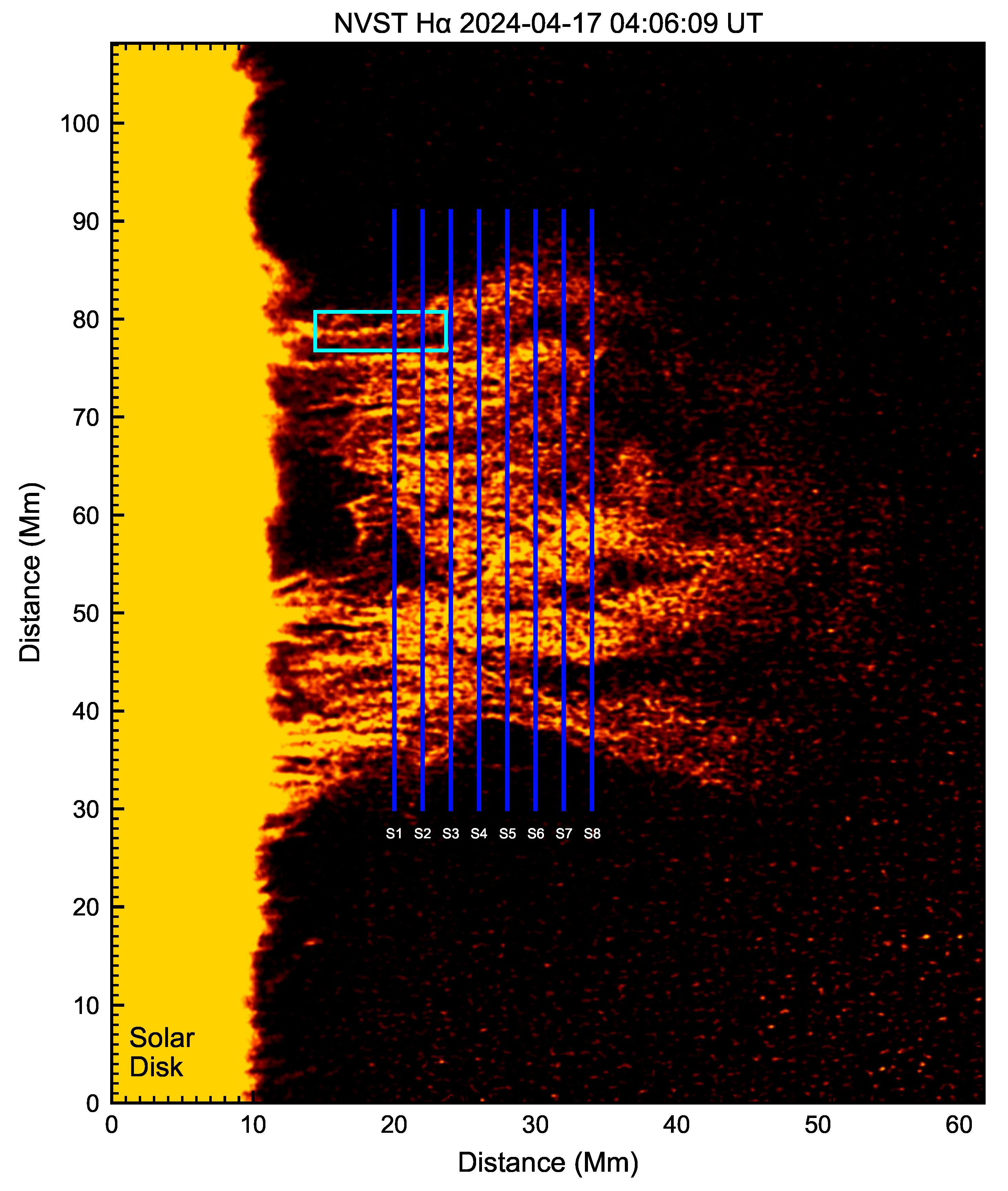
Figure 2.
Time-distance maps along the slits of S1-S8 in Figure 1. The blue dots trace the individual threads with the local maximum intensity. The green lines represent sinusoidal fitting curves. In total, 24 oscillating threads are identified and marked by Thread-1 to Thread-24.
Figure 2.
Time-distance maps along the slits of S1-S8 in Figure 1. The blue dots trace the individual threads with the local maximum intensity. The green lines represent sinusoidal fitting curves. In total, 24 oscillating threads are identified and marked by Thread-1 to Thread-24.
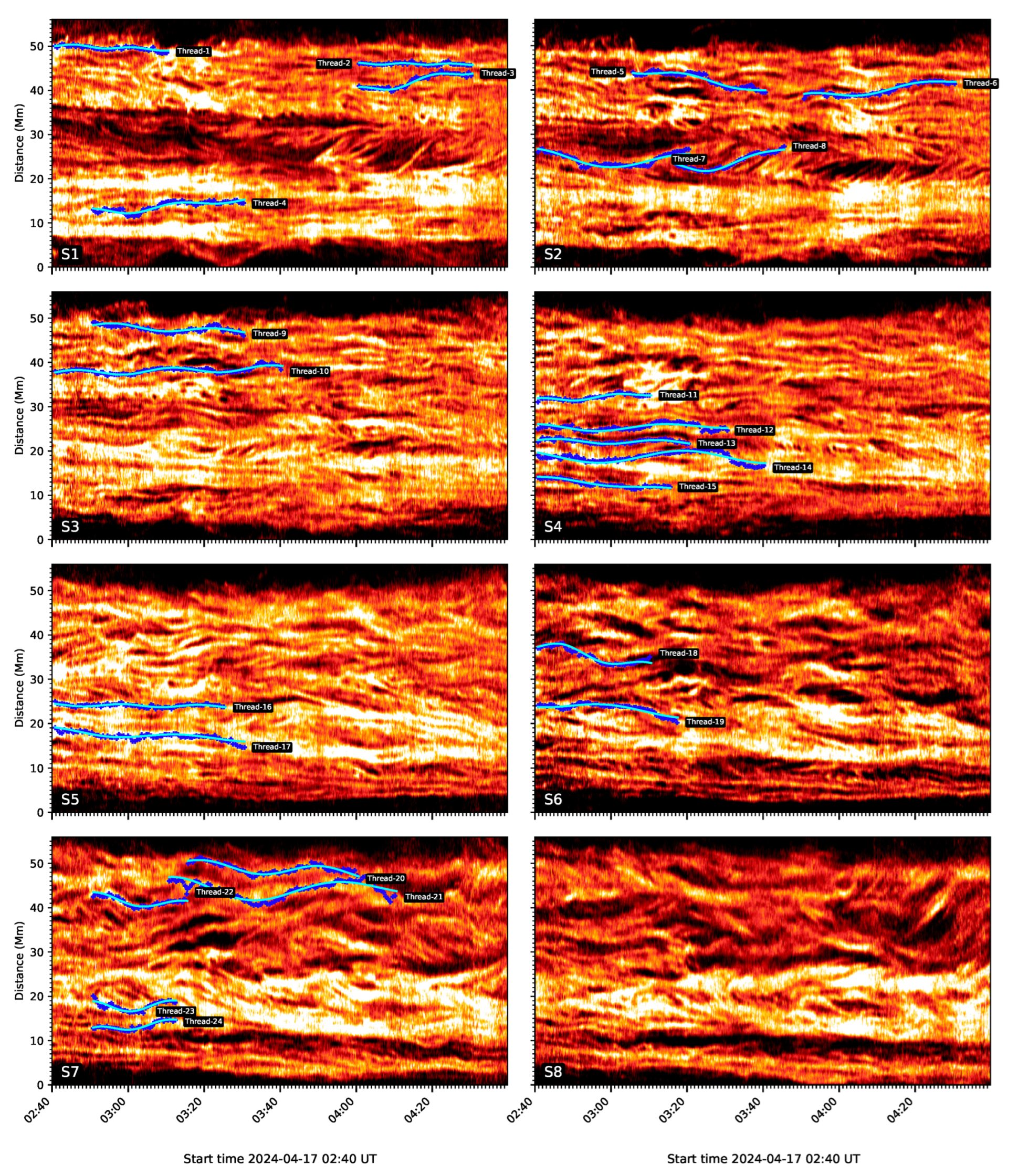
Figure 6.
Histograms of oscillating parameters such as period (a), amplitude (b), drifting speed (c),cycle (d) and lifetime (e) of oscillations. The mean values are given.
Figure 6.
Histograms of oscillating parameters such as period (a), amplitude (b), drifting speed (c),cycle (d) and lifetime (e) of oscillations. The mean values are given.

Disclaimer/Publisher’s Note: The statements, opinions and data contained in all publications are solely those of the individual author(s) and contributor(s) and not of MDPI and/or the editor(s). MDPI and/or the editor(s) disclaim responsibility for any injury to people or property resulting from any ideas, methods, instructions or products referred to in the content. |
© 2025 by the authors. Licensee MDPI, Basel, Switzerland. This article is an open access article distributed under the terms and conditions of the Creative Commons Attribution (CC BY) license (http://creativecommons.org/licenses/by/4.0/).
Copyright: This open access article is published under a Creative Commons CC BY 4.0 license, which permit the free download, distribution, and reuse, provided that the author and preprint are cited in any reuse.


