
Submitted:
16 October 2025
Posted:
17 October 2025
You are already at the latest version
Abstract
In order to characterize topological insulators it is customary to use representations of the electronic structure such as the band structure, where the energy of electrons is represented as a function of their momenta. Topological insulators are then represented as those systems whose surface states have an odd number of crossings at the Fermi level, or, equivalently, as those systems where the spin and momentum is locked at the surface. The density of states, however, cannot in principle be used to distinguish if a material is a topological insulator because it integrates the momentum information for a given energy. In this article, we show that, despite that fact, the density of states of topological insulators show some distinctive characteristics that may even be used to predict if a certain material is of that type or not by using such quantity. We use a series of machine learning algorithms to classify first the density of states and predict then systems with similar densities of states that can lead to new topological materials. We find that, contrary to what would be expected, the densities of states of topological insulators have distinct features that allow to classify and identify these materials according to them. We show that the density of states of topological insulators presents more acute features, which indicates a tendency of these compounds towards more localization.
Keywords:
density of states
; machine learning
; electronic structure
; chemical fingerprints
1. Introduction
Topological insulators (TIs) represent a novel class of quantum materials [1,2] that hold significant promise for next-generation electronic and spintronic devices [3,4]. These materials are characterized by conducting surface states that are spin-polarized and locked to the momentum of the charge carriers, resulting in robust spin-polarized currents that propagate along the surface with minimal dissipation and absence of back-scattering. The identification and characterization of topological insulators typically rely on the analysis of the band structure, which provides explicit information on the momentum and symmetry properties of electronic states.
In contrast, the density of states (DOS) offers no momentum-resolved information, as it corresponds to an energy-dependent quantity obtained by integrating over all -points in the Brillouin zone. As such, the DOS alone does not directly capture the topological nature of materials and is generally considered unsuitable for determining whether a given compound is a topological insulator [5]. Consequently, conventional analysis based solely on the DOS has been limited in this context.
Nevertheless, the DOS has been widely studied using machine learning (ML) techniques in recent years. Various efforts have focused on extracting physical properties from the DOS [6], as well as on the classification and prediction of DOS profiles across diverse material classes [7,8]. Early studies explored the prediction of the DOS at the Fermi level [9], while subsequent work extended this to reconstruct the entire DOS curve [10]. These investigations demonstrated that ML algorithms can predict the shape and features of the DOS with a relatively high degree of accuracy—particularly for restricted families of elements or compounds with specific compositions. However, generalization to broader material spaces remains a challenge, and further progress depends on the availability of larger, high-quality datasets and the development of more powerful learning models.
In this work, we explore how machine learning algorithms can be applied to data extracted from material databases to classify and predict whether a given compound behaves as a topological insulator, based on patterns in its DOS. Our results show that, despite the lack of explicit momentum information in the DOS, certain patterns and characteristics allow for distinguishing topological from non-topological materials with reasonable accuracy. This approach allows us then to uncover hidden relationships in complex materials data and support the discovery of new functional materials for future technologies
The structure of the article is as follows. In Section 2, we describe the dataset used and the machine learning methods employed for classification and prediction. Section 3 presents the results, beginning with the classification performance and followed by DOS predictions for selected materials. In Section 4, we discuss the implications of our findings and assess the viability of using DOS-based representations for identifying topological insulators. Finally, Section 5 summarizes the conclusions and outlines directions for future research.
2. Materials and Methods
2.1. Data Acquisition, Simulation and Preprocessing
To obtain information on the density of states (DOS) of materials, we used the AFLOWLIB materials database [12], one of the largest repositories of computationally investigated materials. Based on data from the ICSD (Inorganic Crystal Structure Database) [13], AFLOW employs the VASP code [14]—based on Density Functional Theory (DFT) [15,16]—to simulate various properties, including DOS, mechanical and electronic characteristics, for 60,392 materials in separate files. All simulations are performed using consistent parameters, allowing reliable comparisons between different compounds.
Due to the impracticality of downloading thousands of files manually, we implemented a Python-based routine to automatically access the HTML content of AFLOW’s web interface and retrieve the relevant DOS files. This process enables the classification and storage of materials ranging from metals to insulators, and from magnetic to non-magnetic systems.
Each downloaded DOS file contains 5,000 values uniformly distributed across the energy range . For our analysis, we focused on a window of , selecting only the values within this interval. In magnetic materials, which show two spin-resolved DOS curves, we summed both channels to obtain the total DOS. Magnetic and non-magnetic materials were treated separately throughout the analysis.
To complement the AFLOW data, we queried the Topological Materials Database [16] to obtain the topological classification of each material. This database contains information for 38,184 materials, including 6,109 topological insulators.
Finally, we applied the following filters to complete the preprocessing stage:
- Only insulating materials were selected, identifiable by the absence of DOS values in a small region around the Fermi level due to the band gap.
- Materials with unknown topological classification were discarded, as the number of materials in AFLOW exceeds those in the Topological Materials Database.
At the end of this process, we obtained a curated dataset containing the DOS and topological classification of each material, ready for further analysis using machine learning techniques.
2.2. Machine Learning Algorithms
The used algorithms can be divided into unsupervised and supervised learning methods. In the first case we used typical classification algorithms such as k-means. These algorithms allow for a fast and relatively accurate classification of elements that belong to different sets or that have different properties. We use then such DOS as initial data to feed the machine learning algorithms.
2.2.1. k-Means++
The clusterization algorithm that we used is known as k-means++ [17], which is an enhanced initialization algorithm for the classic K-means clustering method. It improves the way the initial centroids are chosen, which helps avoid poor clustering results due to unlucky random initialization in standard K-means.
The goal of k-means++ is to spread out the initial centroids, reducing the likelihood of suboptimal solutions and improving convergence. Given a dataset , and a desired number of clusters , the algorithm k-means++ proceeds as follows:
- Choose the first centroid uniformly at random from the data points.
- For each remaining data point compute its distance to the nearest already chosen centroid.
- Choose the next centroid from the data points, where each point is chosen with probability proportional to .
- Iterate the previous steps until k centroids have been chosen.
- Proceed with standard K-means, using these k initial centroids.
This algorithm yields an optimal partitioning for a given k and will be employed to perform unsupervised clustering of the DOS curves from various insulating materials, both topological and non-topological.
2.2.2. PCA Model Reduction
Let us supose that we have a disposal set of m DOS curves corresponding to m different materials, where , where s represents the number of points of each DOS curve.
The PCA model reduction [18], consists in finding an orthogonal basis set of the experimental covariance matrix
where
The matrix C is symmetric and therefore admits an orthogonal diagonalization of the form:
The total variance in the DOS space is given by:
Model reduction consists in finding the index q such as the cumulative energy function
where is a given percentage of the total variance. In summary, PCA seeks to obtain the q-dimensional subspace onto which the data (DOS curves) are projected while preserving of the observed variability.
The projection, of the curve onto the q-dimensional PCA subespace is given by
where are the q eigenvectors associated with the largest eigenvalues of the matrix C.
The reconstruction formula is
where is smooth version of , that is, PCA projection and reconstruction can be viewed as a high frequency filter of the data.
2.2.3. K-Nearest Neighbors (K-NN)
The k-nearest neighbors (K-NN) algorithm is a non-parametric, instance-based method used for classification and regression [19]. The input consists in a dataset of the type: with . Given a query point , the algorithm identifies the set of the k closest training points in the feature space:
where p is the norm used, typically the Euclidean.
In classification, the predicted label is the majority class among the k neighbors:
where is the set of possible classes, and is the indicator function.
In regression, the predicted value is given by the average of the target values of the neighbors:
K-NN is sensitive to the local structure of the data and does not assume any underlying distribution. However, it is computationally intensive at inference time and may suffer from the curse of dimensionality. In our case, it is used combined with dimensionality reduction via PCA.
2.2.4. Bayesian Classifier
A Bayesian classifier is a probabilistic model used in supervised learning that applies Bayes’ theorem to assign a data point characterized by its feature vector to the most probable class . The classification is based on computing the posterior probability of each class given the input data:
where is the posterior probability of class given the input , is the likelihood of observing given class , is the prior probability of class , is the marginal probability of the input.
Since is constant across all classes, the classification rule becomes:
The Naive Bayes classifier, which assumes conditional independence between the features of the input vector , given the class:
This simplification makes the model computationally efficient, even in high-dimensional spaces [20].
2.2.5. Decision Tree Classifier
A Decision Tree is a supervised learning algorithm used for both classification and regression tasks. It represents decisions and their possible consequences in a tree-like structure, where internal nodes correspond to feature-based tests, branches to outcomes of those tests, and leaf nodes to predicted class labels. At each node, the algorithm selects the feature that best splits the data according to a purity criterion. Common impurity measures include entropy and Gini impurity , defined as
and
where is the proportion of instances belonging to class i, and n is the total number of classes [21].
Once the tree is constructed, a new instance is classified by traversing the tree from the root to a leaf node, following the decision rules at each node based on the instance’s feature values.
2.2.6. Support Vector Machines (SVM)
SVM are supervised learning models used for classification and regression tasks. The main idea behind SVM is to find the hyperplane that best separates the data into different classes while maximizing the margin between them.
Given a training dataset of pairs , where is a feature vector and is the class label, the goal is to find a weight vector and a bias b such that the following condition holds for all data points:
The model is trained by solving the following optimization problem:
subject to the constraint above. This finds the hyperplane with the largest margin separating both classes in .
In real-world applications, some misclassifications may be allowed using slack variables and a regularization parameter . This leads to the soft-margin SVM formulation:
subject to
To handle nonlinear classification, SVMs can be extended using the kernel trick, where the dot product is replaced by a kernel function , such as the radial basis function (RBF) or polynomial kernel [22].
2.2.7. Fisher Linear Discriminant Analysis (FLDA)
FLDA is a technique for projecting high-dimensional data onto a one-dimensional subspace in such a way that the separation between two classes is maximized [23].
Suppose we have a dataset consisting of two classes, and , each characterized by its mean vector and , and corresponding scatter matrices, and . The goal is to find the optimal projection vector that maximizes the ratio of between-class variance to within-class variance:
Here, the within-class scatter matrix is defined as:
and the between-class scatter matrix is given by:
The vector that maximizes the criterion is obtained analytically as:
Each sample is then projected onto the subspace spanned by :
where is the coordinate of in . In the binary classification case, the projection yields a scalar value, enabling classification by applying a threshold in the one-dimensional space. In our approach, this scalar feature will be incorporated into the PCA coordinates of each sample in the dataset.
3. Preliminary Analysis
3.1. Distribution of Materials by Topology
Figure 1 shows the distribution of materials in the dataset according to their topological classification—trivial or topological insulator—and their magnetic character. Most topological insulators are non-magnetic, consistent with the role of time-reversal symmetry in stabilizing topological phases. However, a significant number of magnetic topological insulators are also included, reflecting increased interest in these systems.
The dataset is notably imbalanced in the non-magnetic group, where trivial insulators vastly outnumber topological ones. In contrast, magnetic materials are more evenly split between the two classes, indicating that magnetic ordering alone does not determine a material’s topological character. This highlights the need to analyze finer electronic structure features for reliable classification.
These class imbalances—especially in the non-magnetic subset—must be considered when developing machine learning models, as discussed in the next section.
According to structural databases, the Inorganic Crystal Structure Database (ICSD) contains over 210,000 experimentally determined inorganic crystal structures [13]. Based on estimates from comprehensive materials surveys, approximately 5,000 of these are magnetic compounds.
3.2. Distribution by Bravais Lattice
Figure 2 provides a detailed breakdown of the number of materials classified as trivial or topological insulators for each Bravais lattice type, separated by magnetic character.
The distributions vary significantly across lattice types. Among non-magnetic materials, trivial insulators dominate in all lattices, although the relative proportions differ. Topological insulators are most frequently found in orthorhombic C-centered (ORCC), cubic (CUB), monoclinic C-centered (MCLC), tetragonal (TET), and rhombohedral (RHL) lattices. For instance, in the ORCC lattice, the number of topological insulators is roughly half that of trivial ones, while in the trigonal (TRI) lattice, they are nearly absent.
In magnetic materials, the influence of lattice symmetry is even more pronounced. Topological phases are prevalent in TET, RHL, ORCC, MCLC, and monoclinic primitive (MCL) lattices. Some lattices, such as CUB, ORCC, ORCI, and TET, exhibit a majority of topological insulators, whereas others, like MCL and MCLC, are dominated by trivial ones.
These patterns reveal a clear link between Bravais lattice type, magnetism, and topological behavior. Therefore, lattice symmetry is considered a relevant descriptor and is included among the input features for the machine learning models.
3.3. Median DOS
The first step involves classifying the density of states (DOS) as corresponding to either topological or trivial insulators.
Figure 4 presents the median density of states (DOS) for topological and trivial insulators, classified according to their magnetic status. For non-magnetic materials, trivial insulators exhibit a significantly higher DOS—approximately 2.5 times greater—just below the Fermi level, indicating a higher concentration of occupied electronic states near the valence band edge. Above the Fermi level, trivial insulators display a well-defined band gap of approximately 2.6 energy units (), while topological insulators exhibit a smoother transition characterized by a pronounced valley rather than a sharp gap, suggesting the presence of extended states or band inversion near the conduction band edge. Overall, the average DOS remains consistently higher for trivial insulators, possibly reflecting broader band dispersion or the lack of symmetry-protected states in the gap region.
Figure 3.
Graphical representation of the median DOS for non-topological and topological insulators.
Figure 3.
Graphical representation of the median DOS for non-topological and topological insulators.
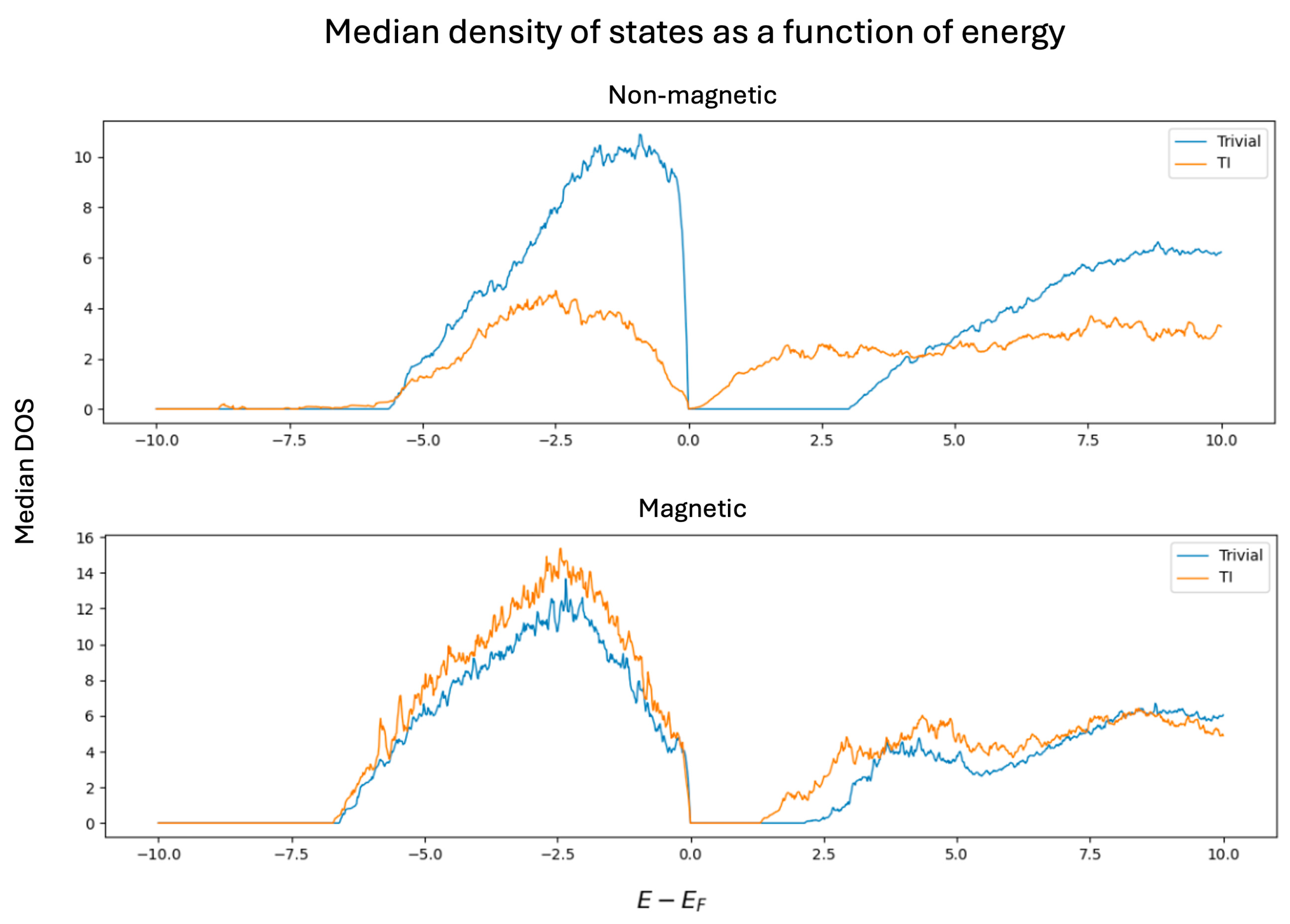
Figure 4.
Graphical representation of the median DOS for non-topological and topological insulators.
Figure 4.
Graphical representation of the median DOS for non-topological and topological insulators.
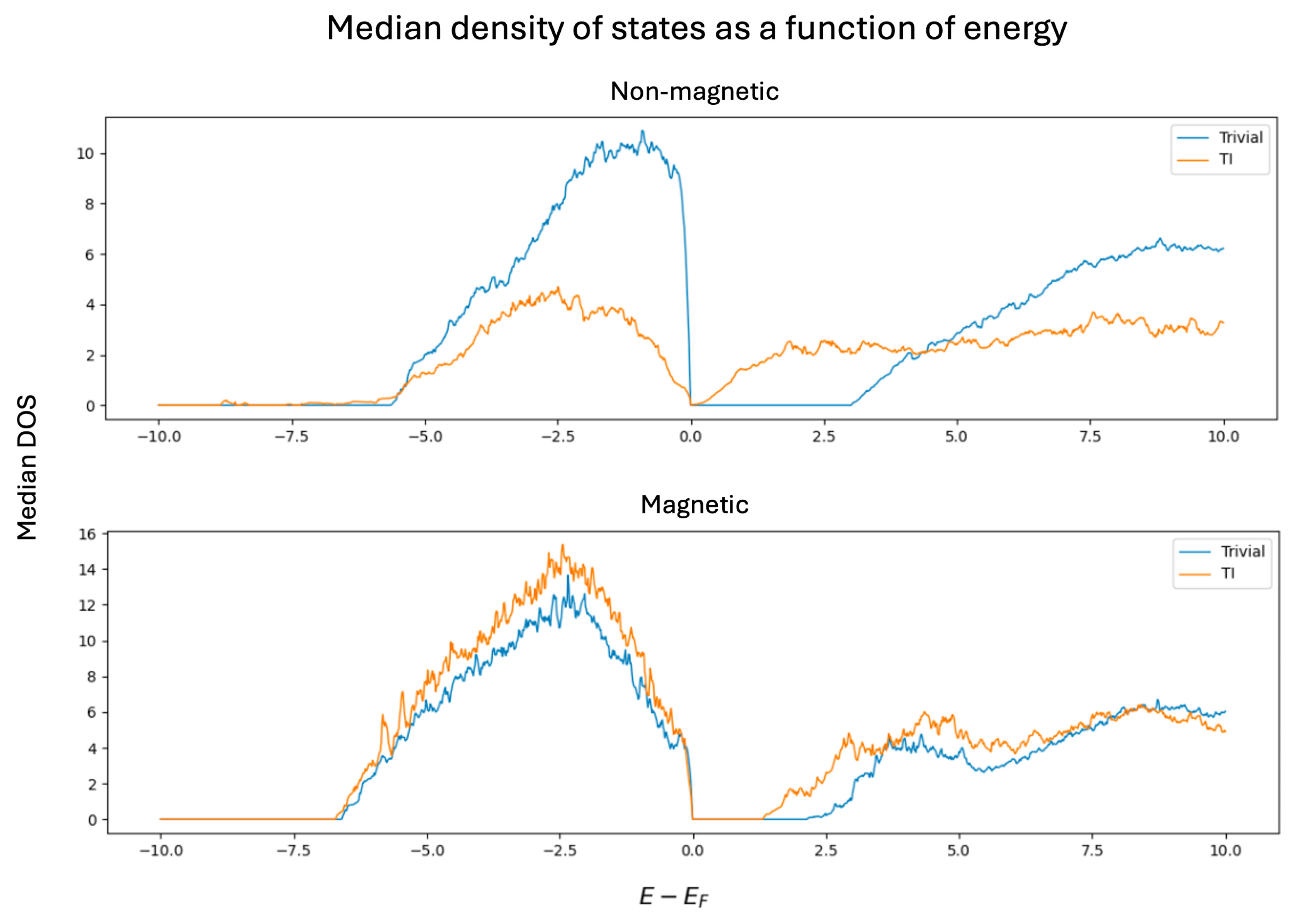
In contrast, for magnetic materials, the average DOS curves for topological and trivial insulators are qualitatively similar in shape. However, the DOS of topological insulators remains slightly higher both below and above the Fermi level. Furthermore, topological insulators in this class exhibit a smaller energy gap—approximately energy units compared to the energy units observed in their trivial counterparts. This reduction in the gap size may be attributed to the breaking of time-reversal symmetry induced by magnetic ordering, which modifies the band topology and can partially close or reshape the gap. Additionally, magnetic interactions can influence spin-orbit coupling effects, potentially reducing the effectiveness of the mechanisms that stabilize large band gaps in non-magnetic topological phases.
A preliminary conclusion is that distinguishing between magnetic topological and trivial insulators is considerably more challenging than in the non-magnetic case, due to the high similarity in their average density of states (DOS) profiles. However, the purpose of applying advanced machine learning techniques—beyond simple statistical comparisons—is to extract latent features and capture non-obvious patterns embedded in the DOS curves. These representations may reveal subtle but systematic differences that can improve the classification performance and provide physical insights into the underlying mechanisms distinguishing the two classes.
The next step is to relate the classification with physical properties that may explain the trends identified by the average DOS curves. A key observation is that the narrower spread of states in topological insulators (TIs) suggests greater electronic localization. This points to bonding types that favor localized bulk states—often associated with insulating behavior—while allowing conductive surface states, which is a hallmark of topological insulators [1,2]. Such localization is typically linked to ionic bonding, where electrons are concentrated around atoms, in contrast to covalent bonds that promote delocalization. Materials with strong ionic character often behave as insulators or semiconductors in the bulk, but can host conductive surface states, especially when surface reconstructions or dangling bonds are present [24]. However, purely ionic materials may lack the necessary surface states if no dangling bonds are formed, meaning that a partial covalent character is also important [25].
Therefore, while ionic bonding plays a crucial role in enabling topological surface states, it is not sufficient on its own. This insight helps narrow down the types of materials likely to exhibit topological insulating behavior, even if a complete topological characterization still requires an analysis of band structure, such as the presence of an odd number of surface band crossings [26,27]. This analysis provides valuable information on the type of materials that have potential to behave as TI.
4. Models for Predicting the Topology of Insulating Materials
The aim of this section is to build a machine learning model capable of predicting whether an insulator is topological or non-topological based on the material’s density of states in the vicinity of the Fermi energy and its Bravais lattice.
4.1. PCA k-NN
In this section, Principal Component Analysis (PCA) is carried out to reduce the dimensionality of the data and KNN on the PCA space to perform the binary classification (TI or trivial).
As mentioned earlier, the downloaded files contained 5,000 values of the density of states (DOS) for each material, all equally spaced in the interval . Since only the DOS values within the interval were later selected, the number of dimensions was reduced to 1,333.
In the case of non-magnetic materials, due to the imbalance between the two classes, where it was observed that the vast majority are non-topological insulators, the principal components basis is computed using only the topological insulators. Then, all materials (both topological and non-topological) are projected onto this basis set. This approach captures as much information as possible from the minority class (topological insulators), attempting to mitigate the data imbalance. For magnetic materials, since both classes are balanced, PCA is performed using all of them.
A common question when applying Principal Component Analysis (PCA) is how many principal components (PCs) should be retained. This can be addressed by examining both the explained variance ratio and the cumulative explained variance. Figure 5 displays the percentage of variance explained by each PC, sorted in descending order. The cumulative curve allows us to determine the number of components needed to capture most of the variability in the data. Based on this analysis, we retain only the first 25 PCA components, which account for of the total variance in non-magnetic materials and in magnetic ones. This represents a substantial dimensionality reduction—from 1,333 original features to just 25 components, or less than of the initial feature space.
To assess the impact of dimensionality reduction, Figure 6 presents the reconstruction of the DOS curves using the first 25 principal components (PCs). As shown, the reconstructed curves closely approximate the original median DOS profiles, indicating that these components successfully capture the overall structure of the data. Including additional components would progressively improve the reconstruction by encoding finer details. In the theoretical limit where all PCs are retained, the reconstruction would be exact. Among the four reconstructed cases, the largest deviation is observed for non-magnetic trivial insulators. This is expected, as the PCA basis for non-magnetic materials was computed using only topological insulators, due to class imbalance. Consequently, projecting trivial insulators onto this basis results in a slightly greater information loss compared to a basis constructed from the full non-magnetic dataset. Nonetheless, this approach favors the minority class, which is advantageous in the context of imbalanced classification.
Figure 7 shows the classification accuracy of the K-NN model as a function of the number of PCs used as features, separately for magnetic and non-magnetic materials, as evaluated through cross-validation. Interestingly, model performance tends to degrade as the number of PCs increases. This behavior stems from the fact that the leading principal components capture the most relevant variance in the data, while subsequent components often encode noise or redundant information, which may hinder model performance. Thus, selecting an appropriate number of PCs is essential for achieving optimal results. The highest accuracies were obtained using 50 PCs: for non-magnetic and for magnetic insulators. Increasing the number of PCs beyond this point does not lead to performance gains. This suggests that high-frequency features in the DOS curves—encoded by higher-order PCs—may introduce ambiguity, thereby reducing classification reliability. On the other hand, retaining only the first 25 PCs appears insufficient to construct accurate models. Lastly, the performance gap between the two cases is attributed to the strong class imbalance in the non-magnetic dataset, which limits the model’s ability to generalize.
Figure 8 shows the 10th and 90th percentiles of the projection coordinates of the DOS curves of topological insulators onto the PCA basis, separately for magnetic and non-magnetic systems. These curves are constructed by projecting the DOS of known topological insulators onto the PCA basis and then computing, for each principal component, the 10th and 90th percentiles of the resulting coefficients. Percentiles are preferred over extrema (minimum and maximum) as they provide smoother and more robust bounds, reducing the influence of outliers.
This construction effectively characterizes the typical variation of the DOS of topological insulators in the reduced PCA space. By selecting values within the interval defined by the percentile bounds for each component, one can reconstruct synthetic DOS curves through the inverse PCA transformation. These generated DOS profiles represent hypothetical materials whose electronic structures resemble those of known topological insulators.
If a real material exhibits a DOS similar to one of these generated profiles, it is likely to be a strong candidate for being a topological insulator. This approach can thus be used as a tool to explore and identify new topological materials based on their density of states, leveraging the statistical features extracted from known cases.
4.2. Fisher’s Linear Discriminant Analysis (LDA)
After completing all PCA-related analyses, Fisher’s Linear Discriminant Analysis (LDA) is applied to the original data. This technique projects the data onto a direction that maximizes the separation between class means while minimizing the variance within each class, thereby enhancing class discriminability. The resulting one-dimensional projections are incorporated as an additional feature for subsequent machine learning tasks.
At this stage, a complete data matrix X is constructed, comprising all the input variables: the Bravais lattice encoding, the first 25 principal components, and the Fisher LDA projections. Accompanying this matrix is a label vector , indicating the topological classification of each material (i.e., trivial or topological insulator). Together, X and form a well-structured dataset suitable for training supervised machine learning models.
4.3. Topology Prediction of Insulating Materials
In all numerical experiments, the dataset was split into two distinct subsets: a training set comprising of the data, and a test set containing the remaining . It is crucial to ensure that the distribution of topological classes in the test set reflects that of the training set. Otherwise, the model would be evaluated on data whose statistical properties differ significantly from those it was trained on, leading to biased or unreliable performance metrics.
Magnetic and non-magnetic materials are treated as separate cases throughout the study. Consequently, independent models are trained and evaluated for each subset to account for their distinct physical characteristics and classification challenges.
4.3.1. Magnetic Materials
k-NN
We start by building a k-Nearest Neighbors (kNN) model for the magnetic materials. This model requires tuning several parameters: the number of neighbors k, the distance metric, and the weighting of neighbors (equal or distance-based influence).
The chosen distance metric is the Minkowski metric, which depends on a parameter p:
To find the best values for k, p, and the weighting scheme, a cross-validation process is performed using the following ranges:
- Number of neighbors (k): 1, 3, 5, 7, 9, 11.
- Parameter p: 1, 2, 3, 4, 5, 6.
- Weighting: Uniform or distance-based.
With 6 values for k, 6 for p, and 2 weight options, there are parameter combinations. Using 3-fold cross-validation, a total of models are evaluated to select the best-performing configuration.
The findings can be summarized in the following key conclusions:
- When using uniform weighting, the highest accuracy is obtained with a single neighbor (), and .
- With distance-based weighting, the performance is more consistent across different parameter combinations.
- The best overall results are achieved with , , and distance-based weighting. This configuration yields an accuracy of on the training set and on the test data.
The confusion matrix for the best classifier is shown in Figure 9.
Bayesian Classifier
After training the model to compute the corresponding prior probabilities and likelihoods, it is applied to the test data, resulting in Figure 10. The obtained accuracy is , very similar to that achieved by the kNN model. However, an increase in the number of false negatives is observed (twice that of the kNN model), and a considerable reduction in the number of false positives.
Decision Tree
When constructing the decision tree, cross-validation is employed to select the optimal tree depth, with candidate values of 1, 3, 5, and 7. Figure 11 displays the best-performing tree obtained through this tuning process.
As shown, the resulting decision tree has a depth of 3 and includes 8 terminal nodes (leaves). Notably, several internal nodes use the feature derived from Fisher’s Linear Discriminant, highlighting its relevance in the classification task. The model achieves an accuracy of on the test set, which is approximately 10 percentage points higher than both the k-NN and Bayesian classifiers.
Support Vector Machine
Finally, a Support Vector Machine (SVM) classifier is constructed. As with previous models, cross-validation is employed to optimize its hyperparameters: the regularization parameter , which controls the trade-off between maximizing the margin and minimizing classification errors; the choice of kernel function; and any additional parameters associated with the selected kernel.
The best performance was achieved using a linear kernel with . This model yielded an accuracy of on the test set, comparable to the performance of the decision tree classifier. The fact that the optimal kernel is linear suggests that the data is approximately linearly separable in the feature space.
4.3.2. Non-Magnetic Materials
In the case of non-magnetic materials, it is crucial to address the strong class imbalance when training machine learning models, as they are prone to favor the majority class (trivial topology). For instance, in an extreme scenario where a model entirely ignores the minority class and always predicts the majority, the resulting accuracy may appear high due to class prevalence, yet the model would fail to capture meaningful patterns in the minority class, rendering it ineffective for its intended purpose.
Consequently, in imbalanced classification problems, it is essential to prioritize the model’s ability to correctly predict the minority class. For this reason, accuracy alone is no longer a sufficient metric to assess model performance. Although it will still be reported, additional metrics will be introduced in the next section to provide a more informative evaluation. The modeling strategy mirrors that employed for magnetic materials: constructing a kNN model, a Bayesian classifier, a decision tree, and a support vector machine. For the kNN classifier, cross-validation identifies the optimal parameters as , , and distance-based weighting. This configuration achieves a test accuracy of . The Bayesian classifier attains an accuracy of . As before, one of its key advantages is computational efficiency: despite the larger dataset for non-magnetic materials, the model is trained and evaluated with minimal computational cost. Finally, the optimal support vector machine, again selected via cross-validation, uses the same configuration as in the magnetic case, with a linear kernel, achieving a test accuracy of .
4.4. Summary
Table 1 shows different metrics (accuracy, precision, Recall and F1 Score) for each of the models built for the magnetic, in order to make an objective comparison and determine which one performs the best materials.
Using accuracy as the primary evaluation metric, both the decision tree and support vector machine (SVM) models demonstrate strong performance, correctly predicting nearly 90% of the materials—approximately ten percentage points higher than the kNN and Bayesian classifiers. Among these, the decision tree slightly outperforms the SVM in terms of accuracy. When considering the F1 score as an alternative metric, the decision tree also achieves the highest value. Based on both metrics, we conclude that the decision tree is the most suitable model for predicting the topology of new magnetic insulators. It is worth noting that the optimal decision tree has a depth of 3 levels and 8 leaf nodes. Moreover, in five of its decision nodes, the variable derived from Fisher’s linear discriminant is used, underscoring the relevance of that analysis in guiding the construction of the final model.
Regarding the non-magnetic materials, Table 2 shows the same metrics for all the machine learning models used in this paper.
As previously discussed, accuracy is consistently high across all models in this case due to the class imbalance in the dataset. However, this metric alone does not adequately reflect model quality. Therefore, it is necessary to consider alternative evaluation criteria. One such metric is the F1 score, which balances both recall and precision. According to this measure, the best-performing models are clearly the kNN and the decision tree. Another particularly informative metric is recall, especially for the minority class (topological insulators), which is the primary target for correct classification. The kNN model achieves the highest recall, nearly , indicating that it correctly identifies 8 out of every 10 actual topological insulators, misclassifying only 2 as trivial insulators. These results are promising, as the model successfully detects the majority of topological insulators. Nevertheless, further improvements could be pursued to increase this recall even more.
5. Discussion
Through the analysis of a comprehensive materials database, we identified topological insulators (TIs) based on criteria established by our classification models. This approach enabled not only the confirmation of known trivial insulators but also the prediction of new candidate TIs. Comparisons between the predicted and previously reported TIs demonstrated a high level of consistency, underscoring the validity of using the density of states (DOS) as an informative descriptor—despite its lack of explicit momentum dependence.
Notably, a subset of ceramic compounds, typically characterized by insulating behavior due to predominantly ionic and partially covalent bonding, was also classified as topological. These materials, while chemically and structurally diverse, share common physical attributes such as high hardness and electrical resistivity. This suggests that certain macroscopic properties—independent of detailed chemical composition—may correlate with non-trivial topological phases. Such findings highlight the potential of machine learning not only to reproduce established insights but also to uncover previously unrecognized physical patterns beyond the DOS, pointing to new descriptors worth exploring in future studies. For instance, the tendency of TIs to exhibit localized states could correlate with features such as the bandgap magnitude or susceptibility to external perturbations.
Conversely, our models also identified features that are typically incompatible with topological phases. Materials with delocalized electronic states and broad DOS profiles—often associated with strong covalent bonding—rarely exhibit topological insulating behavior. Although these compounds may remain insulating, their DOS characteristics alone often suffice to exclude them from TI classification. This filtering capability is particularly valuable, as it provides a computationally inexpensive way to discard unlikely candidates without requiring complex ab initio calculations.
The use of DOS-based machine learning models thus offers a promising route for efficient pre-screening of materials and illustrates that descriptors previously deemed insufficient can yield surprisingly rich insights when processed through suitable learning algorithms. Furthermore, this reinforces the idea that not all conventional descriptors are indispensable: relevant information can often be inferred indirectly through simpler fingerprints.
Once the classification and feature selection stages are complete, the next logical step is to use the extracted knowledge to guide the discovery of new compounds. To that end, we trained regression models on selected subsets of the data, using the output of the classification phase in combination with additional material descriptors to predict TI-relevant properties. Although various machine learning approaches are feasible, regression-based techniques proved particularly suitable given the structure of our dataset and the nature of the prediction task.
The descriptors considered include elemental identity, atomic radius, valence electron count, and electronegativity—parameters previously validated for their impact on electronic structure. Among these, the combination of Bravais lattice and elemental type was especially informative, as it reflects both geometric and compositional characteristics of the material. When complemented with atomic and electronic descriptors, the predictive power of the model improved substantially.
These features enabled the inference of links between electronic, structural, and even mechanical properties. The accuracy of the resulting predictions hinges on both the quality and relevance of the selected fingerprints. In this context, it is crucial that the descriptor set be tailored to the target property: predictions of electronic behavior, for instance, benefit from inputs related to symmetry, valence configuration, and bonding type.
In general, the machine learning models used in this study learned statistical mappings from descriptors to target labels or values. While different algorithms may exhibit slightly different performance, most achieved comparable results. Our focus was on selecting models that strike a balance between predictive accuracy and computational cost.
Overall, this work demonstrates that even relatively simple machine learning methods, when trained on meaningful physical descriptors like the DOS and Bravais lattice, can provide valuable insights and accelerate the search for new topological materials.
6. Conclusions
This study demonstrates that, contrary to conventional wisdom, the density of states (DOS) contains exploitable features that allow reliable classification of topological insulators (TIs) using machine learning (ML) techniques. While the DOS integrates out momentum information and is typically not used to characterize topological phases, our analysis shows that it exhibits latent patterns—such as sharper peaks and indications of localization—that are distinct in TIs and can be systematically identified through data-driven methods.
By combining DOS profiles with basic structural descriptors like the Bravais lattice, we developed a classification pipeline capable of distinguishing between trivial and topological insulators across both magnetic and non-magnetic materials. Dimensionality reduction via PCA and LDA effectively captured the essential variance and class separability in the DOS data, enabling classifiers such as SVMs, kNN, and decision trees to achieve accuracies above 85–90
Our results indicate that localized electronic features, often linked to ionic or partially covalent bonding, correlate with topological behavior, particularly in ceramics and complex oxides. This supports the idea that some physical properties relevant to topology may transcend chemical complexity, providing a physical basis for simplified screening strategies. Conversely, materials with delocalized states and broad DOS features—characteristic of strong covalent bonding—are consistently ruled out as TIs, reinforcing the utility of DOS-based descriptors for efficient filtering.
Beyond classification, we also demonstrate that synthetic DOS profiles generated in reduced-dimensional spaces can be used to explore and propose new candidate materials. This bridges the gap between data-driven prediction and exploratory materials discovery, offering a scalable approach to identify topological compounds before engaging in computationally intensive ab initio validation.
In summary, this work shows that machine learning applied to minimal input features—DOS and lattice symmetry—can not only replicate known trends in topological materials but also uncover hidden patterns and descriptors. These findings suggest that descriptors once considered insufficient, like the DOS, may hold untapped predictive power when paired with appropriate ML techniques. Future work may extend this framework by incorporating ensemble models, exploring broader descriptor sets, or applying generative techniques for inverse design. Ultimately, this approach accelerates the discovery of quantum materials by shifting the paradigm toward interpretable, lightweight, and physically grounded prediction models.
Author Contributions
Conceptualization, Z.F.M, J.L.F.M. and V.M.G.S.; methodology, Z.F.M, J.L.F.M. and V.M.G.S.; software, A.D.N., J.L.F.M. and V.M.G.S; validation, A.D.N., Z.F.M, J.L.F.M. and V.M.G.S; formal analysis, A.D.N., Z.F.M, J.L.F.M. and V.M.G.S; investigation, A.D.N., Z.F.M, J.L.F.M. and V.M.G.S; resources, A.D.N., J.L.F.M. and V.M.G.S; data curation, A.D.N., Z.F.M, J.L.F.M. and V.M.G.S; writing—original draft preparation, A.D.N., Z.F.M, J.L.F.M. and V.M.G.S; writing—review and editing, A.D.N., Z.F.M, J.L.F.M. and V.M.G.S; supervision, A.D.N., Z.F.M, J.L.F.M. and V.M.G.S. All authors have read and agreed to the published version of the manuscript.
Funding
This research received no external funding.
Conflicts of Interest
The authors declare no conflicts of interest.
References
- Hasan, M.Z.; Kane, C.L. Colloquium: Topological insulators. Reviews of Modern Physics 2010, 82, 3045–3067. [Google Scholar] [CrossRef]
- Qi, X.-L.; Zhang, S.C. Topological insulators and superconductors. Reviews of Modern Physics 2011, 83, 1057–1110. [Google Scholar] [CrossRef]
- Moore, J.E. The birth of topological insulators. Nature 2010, 464, 194–198. [Google Scholar] [CrossRef]
- Pesin, D.; MacDonald, A.H. Spintronics and pseudospintronics in graphene and topological insulators. Nature Materials 2012, 11, 409–416. [Google Scholar] [CrossRef]
- Vergniory, M.G.; Elcoro, L.; Felser, C.; Regnault, N.; Bernevig, B.A.; Wang, Z. A complete catalogue of high-quality topological materials. Nature 2019, 566, 480–485. [Google Scholar] [CrossRef]
- Jha, D.; Ward, L.; Paul, A.; King, W.E.; Wolverton, C.; Agrawal, A. ElemNet: Deep Learning the Chemistry of Materials From Only Elemental Composition. Scientific Reports 2018, 8, 17593. [Google Scholar] [CrossRef] [PubMed]
- Goodall, R.; Lee, A.A. Predicting materials properties without crystal structure: Deep representation learning from stoichiometry. Nature Communications 2020, 11, 6280. [Google Scholar] [CrossRef] [PubMed]
- Schmidt, J.; Marques, M.R.; Botti, S.; Marques, M.A. Recent advances and applications of machine learning in solid-state materials science. npj Computational Materials 2019, 5, 83. [Google Scholar] [CrossRef]
- Rajan, A.C.; Mishra, A.; Satsangi, S.; Vaishnav, S.; Pandey, A.A.; Sarkar, A.D.; Chakraborty, A.; Waghmare, U.V.; Joshi, A.S.; De, R. Machine-learning-assisted accurate band gap predictions of functionalized MXene. Chemistry of Materials 2020, 32, 2954–2963. [Google Scholar] [CrossRef]
- Xie, T.; Grossman, J.C. Crystal Graph Convolutional Neural Networks for an Accurate and Interpretable Prediction of Material Properties. Physical Review Letters 2018, 120, 145301. [Google Scholar] [CrossRef]
- Sánchez Pérez de Amézaga, C.; García-Suárez, V.M.; Fernández-Martínez, J.L. Classification and prediction of bulk densities of states and chemical attributes with machine learning techniques. Applied Mathematics and Computation 2022, 412, 126587. [Google Scholar] [CrossRef]
- Curtarolo, S.; Setyawan, W.; Hart, G.L.W.; Jahnatek, M.; Chepulskii, R.V.; Taylor, R.H.; Wang, S.; Xue, J.; Yang, K.; Levy, O.; Mehl, M.J.; Stokes, H.T.; Demchenko, D.O.; Morgan, D. AFLOW: An automatic framework for high-throughput materials discovery. Computational Materials Science 2012, 58, 218–226. [Google Scholar] [CrossRef]
- FIZ Karlsruhe. Inorganic Crystal Structure Database (ICSD). https://icsd.fiz-karlsruhe.de (Accessed 2025).
- Kresse, G.; Furthmüller, J. Efficient iterative schemes for ab initio total-energy calculations using a plane-wave basis set. Physical Review B 1996, 54, 11169–11186. [Google Scholar] [CrossRef] [PubMed]
- Hohenberg, P.; Kohn, W. Inhomogeneous Electron Gas. Physical Review 1964, 136, B864–B871. [Google Scholar] [CrossRef]
- Kohn, W.; Sham, L.J. Self-Consistent Equations Including Exchange and Correlation Effects. Physical Review 1965, 140, A1133–A1138. [Google Scholar] [CrossRef]
- Arthur, D.; Vassilvitskii, S. k-means++: The Advantages of Careful Seeding. Proceedings of the Eighteenth Annual ACM-SIAM Symposium on Discrete Algorithms, 2007, 1027.
- Hotelling, H. Analysis of a complex of statistical variables into principal components. J. Educ. Psychol. 1933, 24, 417–442. [Google Scholar] [CrossRef]
- Altman, N.S. An Introduction to Kernel and Nearest-Neighbor Nonparametric Regression. The American Statistician 1992, 46, 175–185. [Google Scholar] [CrossRef]
- Zhang, H. The Optimality of Naive Bayes. AA 2004, 1, 3. [Google Scholar]
- Quinlan, J.R. Induction of decision trees. Mach Learn 1986, 1, 81–106. [Google Scholar] [CrossRef]
- Cortes, C.; Vapnik, V. Support-Vector Networks. Machine Learning 1995, 20, 273–297. [Google Scholar] [CrossRef]
- Fisher, R.A. The use of multiple measurements in taxonomic problems. Annals of Eugenics 1936, 7, 179–188. [Google Scholar] [CrossRef]
- Zhang, F.; Kane, C.L.; Mele, E.J. Surface states of topological insulators. Phys. Rev. B 2012, 86, 081303. [Google Scholar] [CrossRef]
- Andrei Bernevig, B.; et al. Quantum Spin Hall Effect and Topological Phase Transition in HgTe Quantum Wells. Science 2006, 314, 1757–1761. [Google Scholar] [CrossRef] [PubMed]
- Fu, L.; Kane, C.L.; Mele, E.J. Topological insulators in three dimensions. Physical Review Letters 2007, 98, 106803. [Google Scholar] [CrossRef]
- Moore, J. The birth of topological insulators. 2010, 464, 194–198. [Google Scholar] [CrossRef]
Figure 1.
Histogram of materials according to their topology.
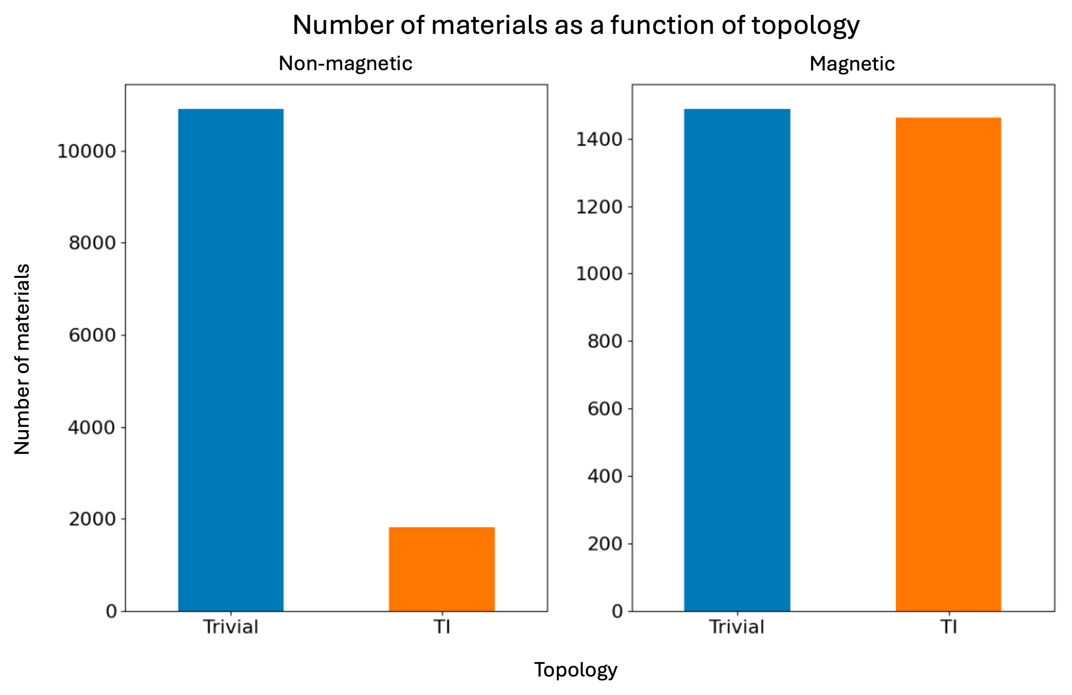
Figure 2.
Histogram of materials according to their topology and Bravais lattice.
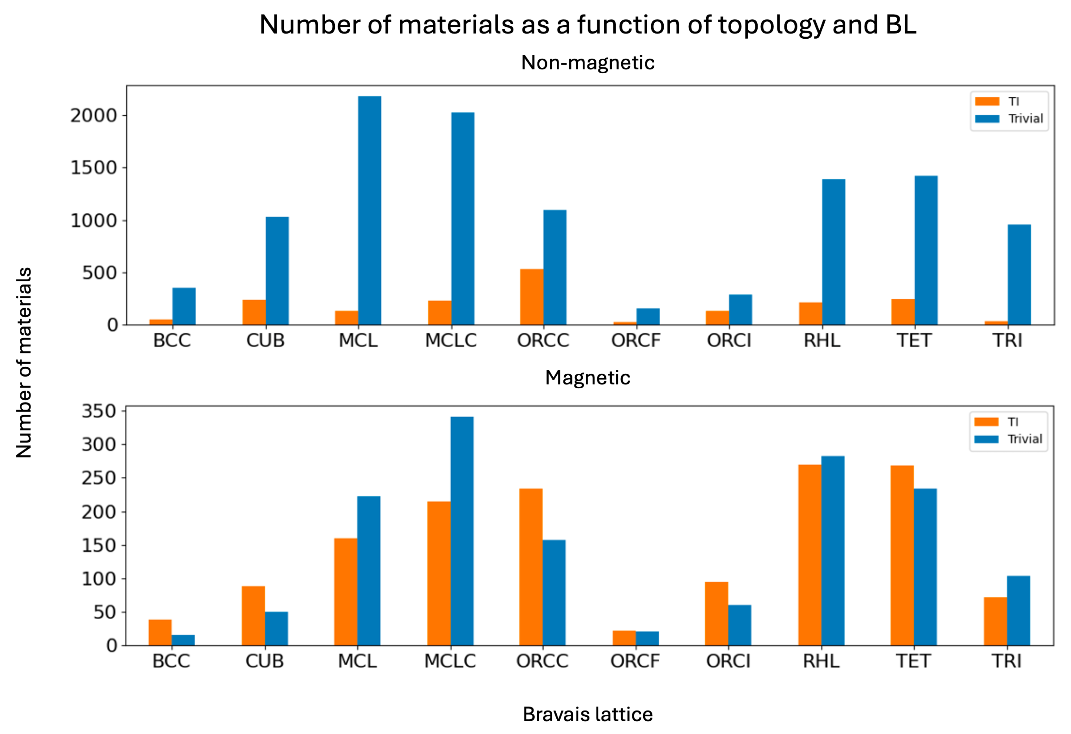
Figure 5.
Percentage of variance and accumulated variance for the first 50 PCAs.
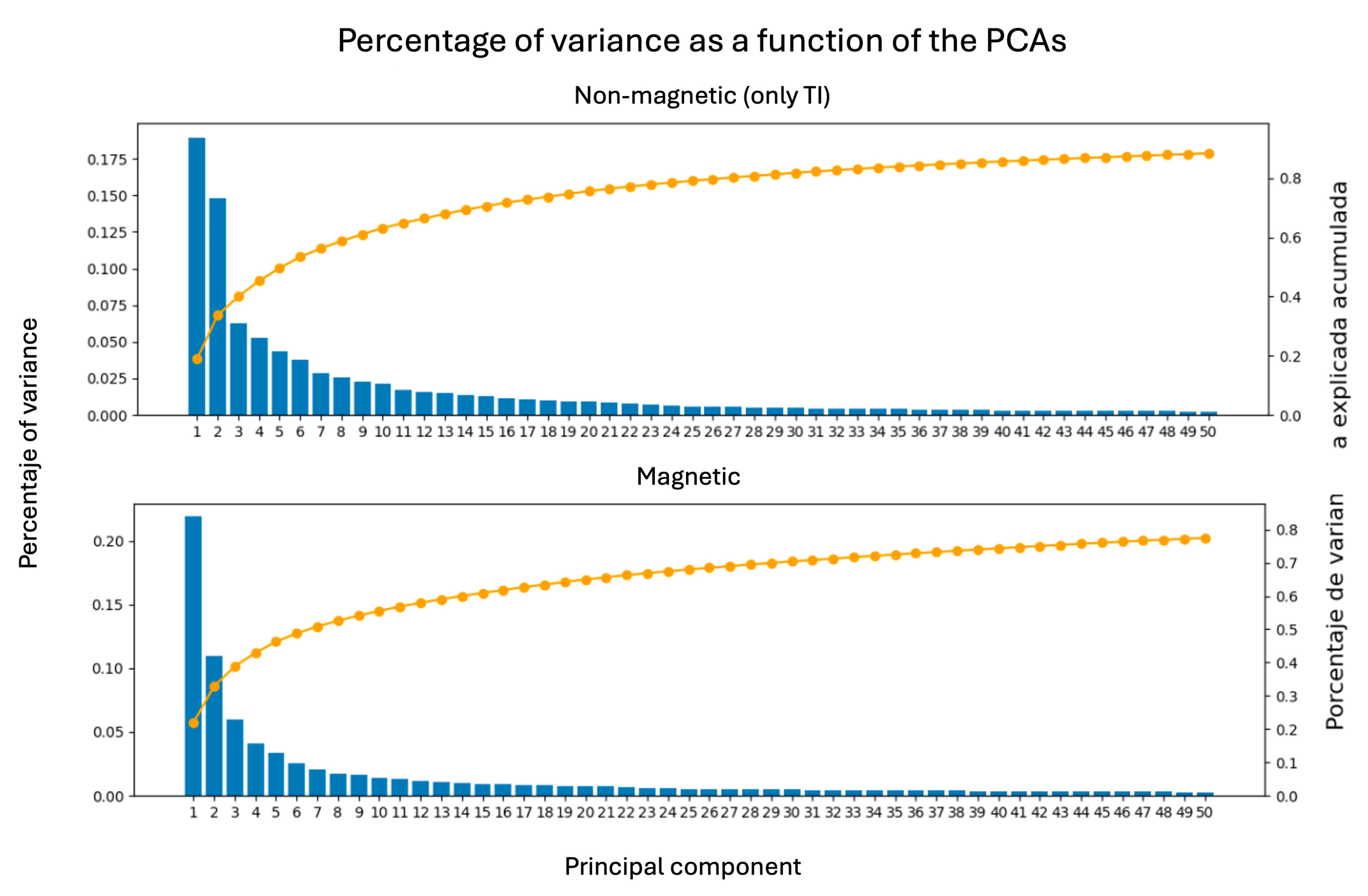
Figure 6.
Reconstruction of the plots of the median of the DOS.
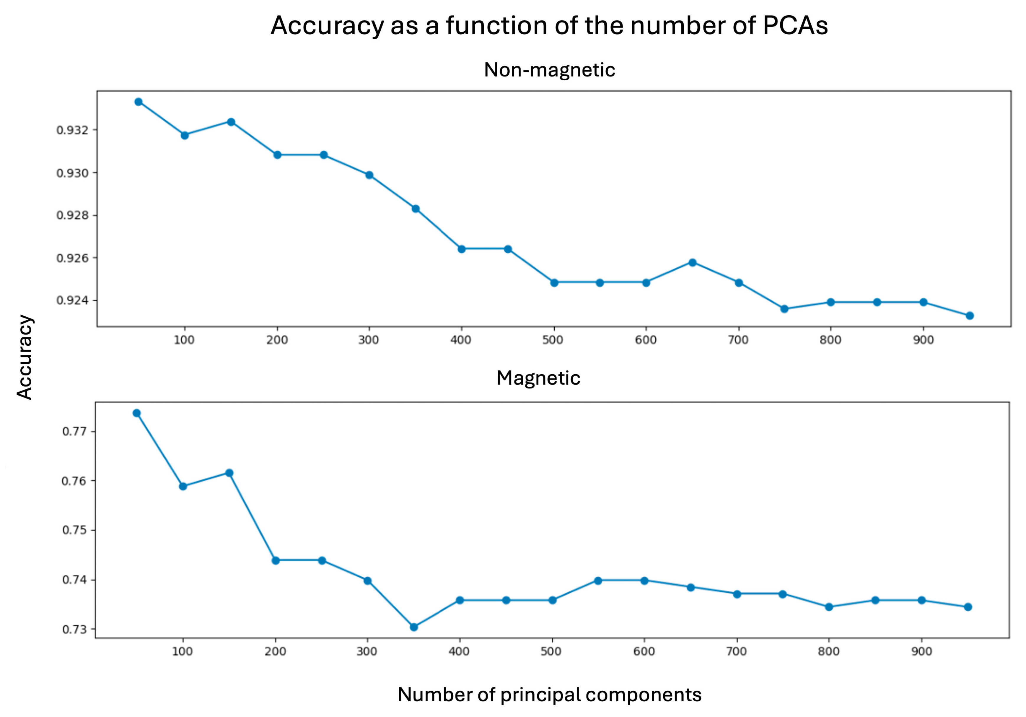
Figure 7.
Accuracy for a kNN model as a function of the number of PCAs used to train it.
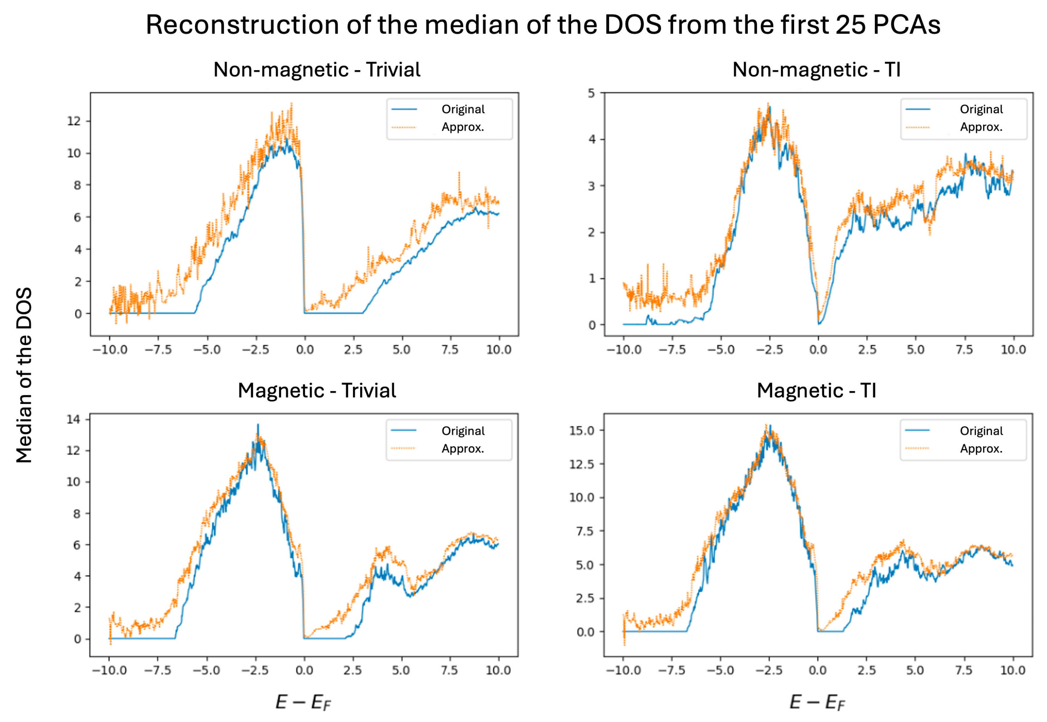
Figure 8.
Percentiles 10 and 90 of the projections of the DOS of the TI on the PCA base.
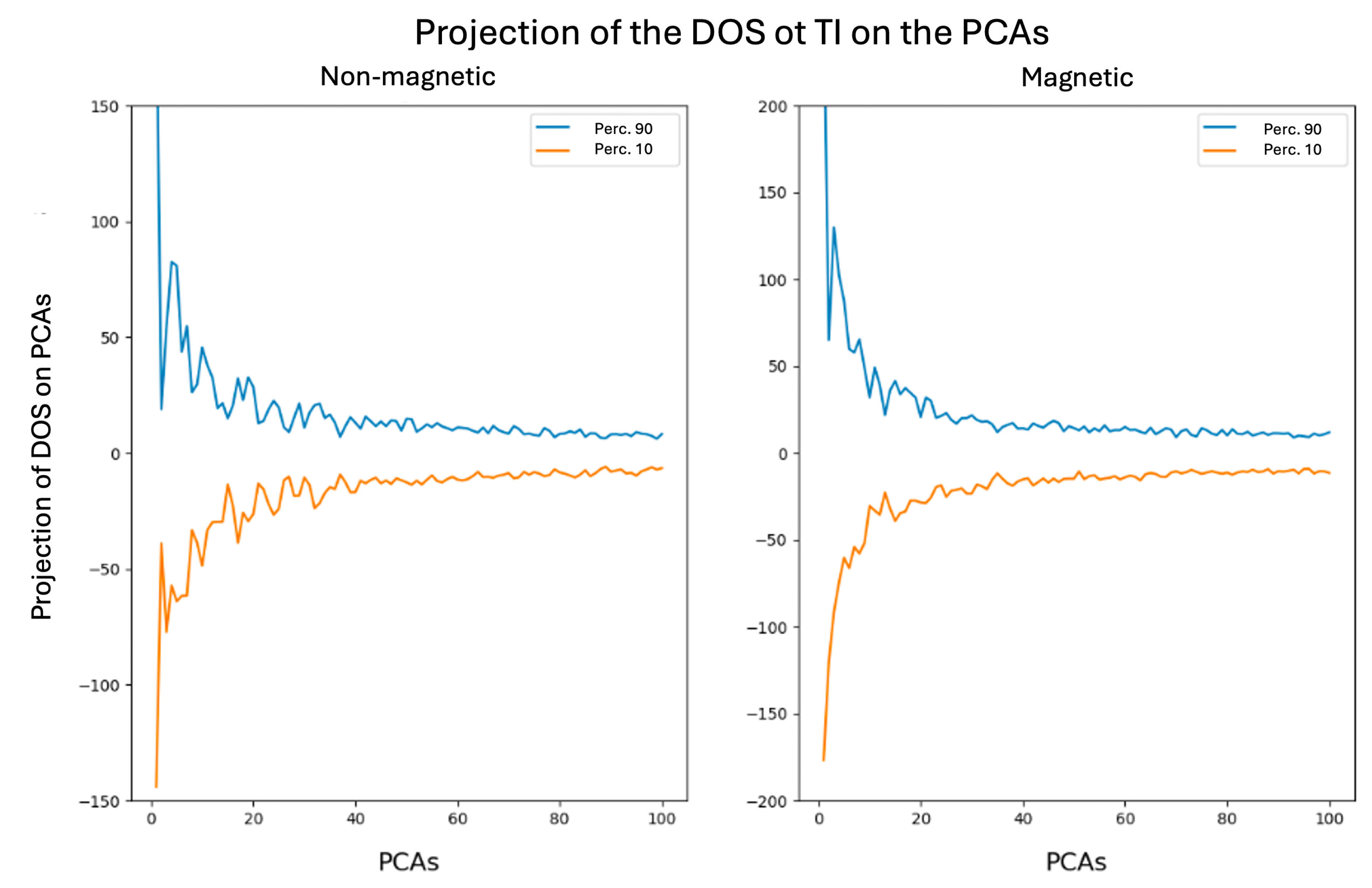
Figure 9.
Confusion matrix for the kNN model in the test.
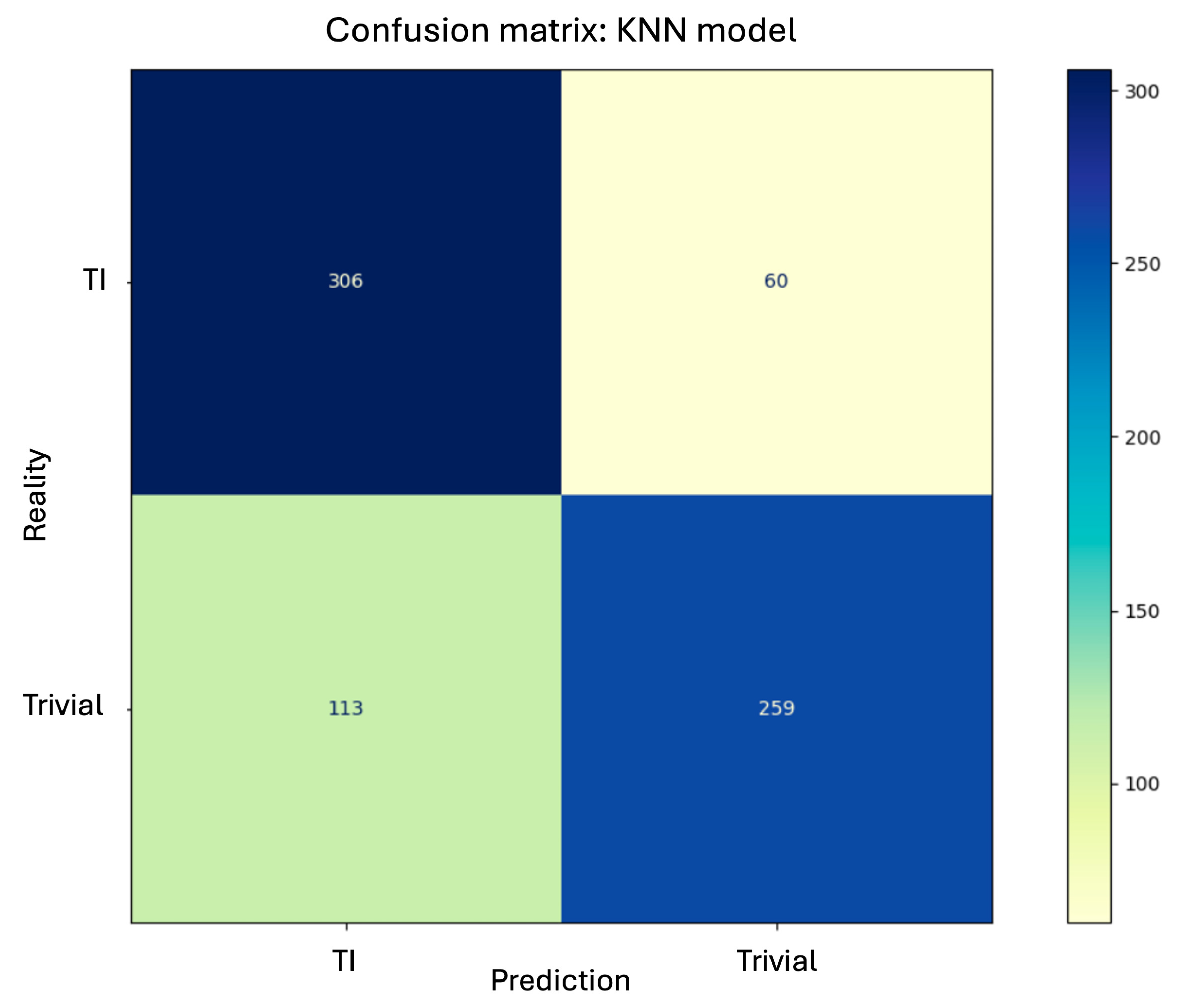
Figure 10.
Confusion matrix for the bayesian classifierl in the test.
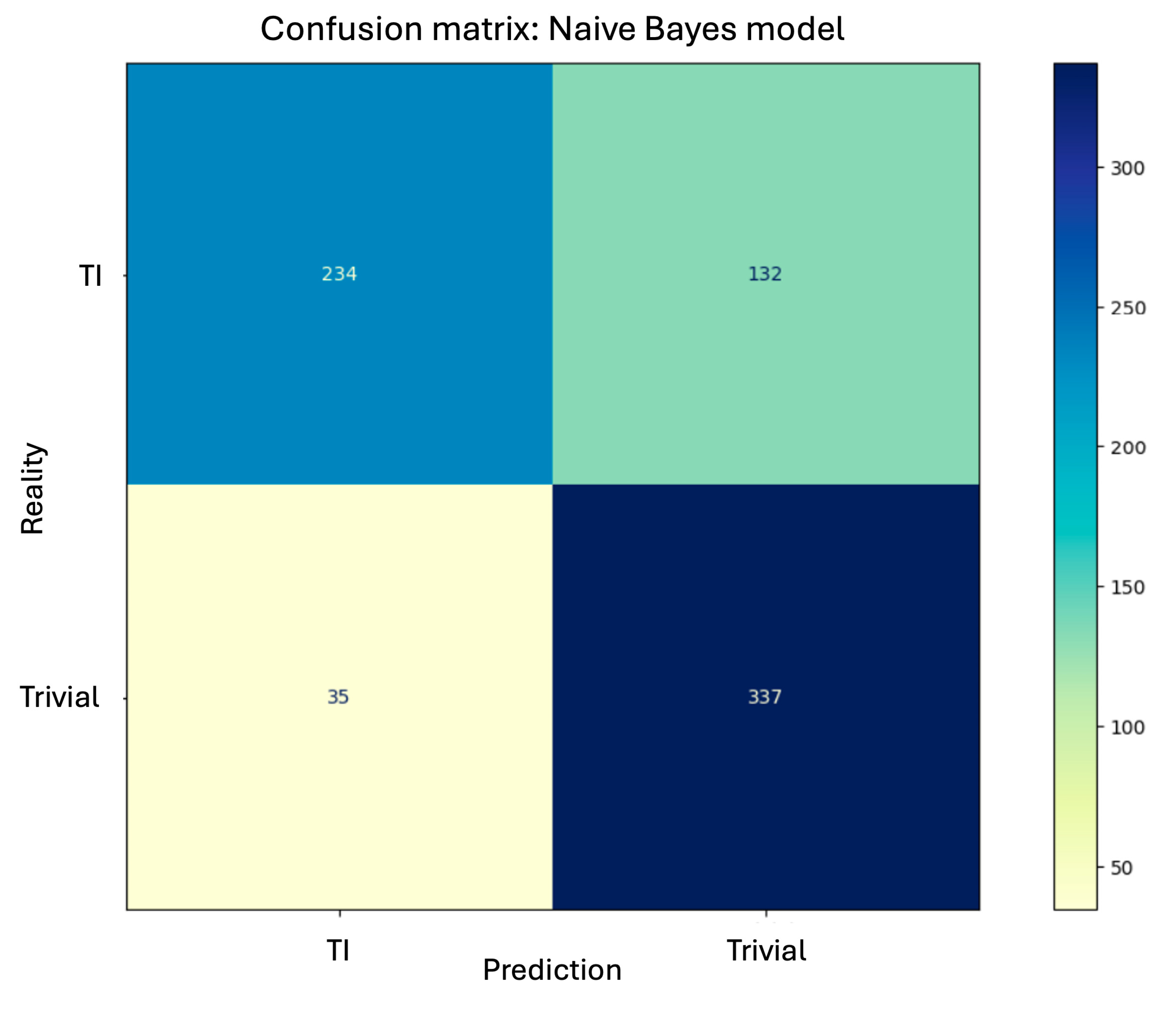
Figure 11.
Decision tree built to predict the topology of the magnetic materials.
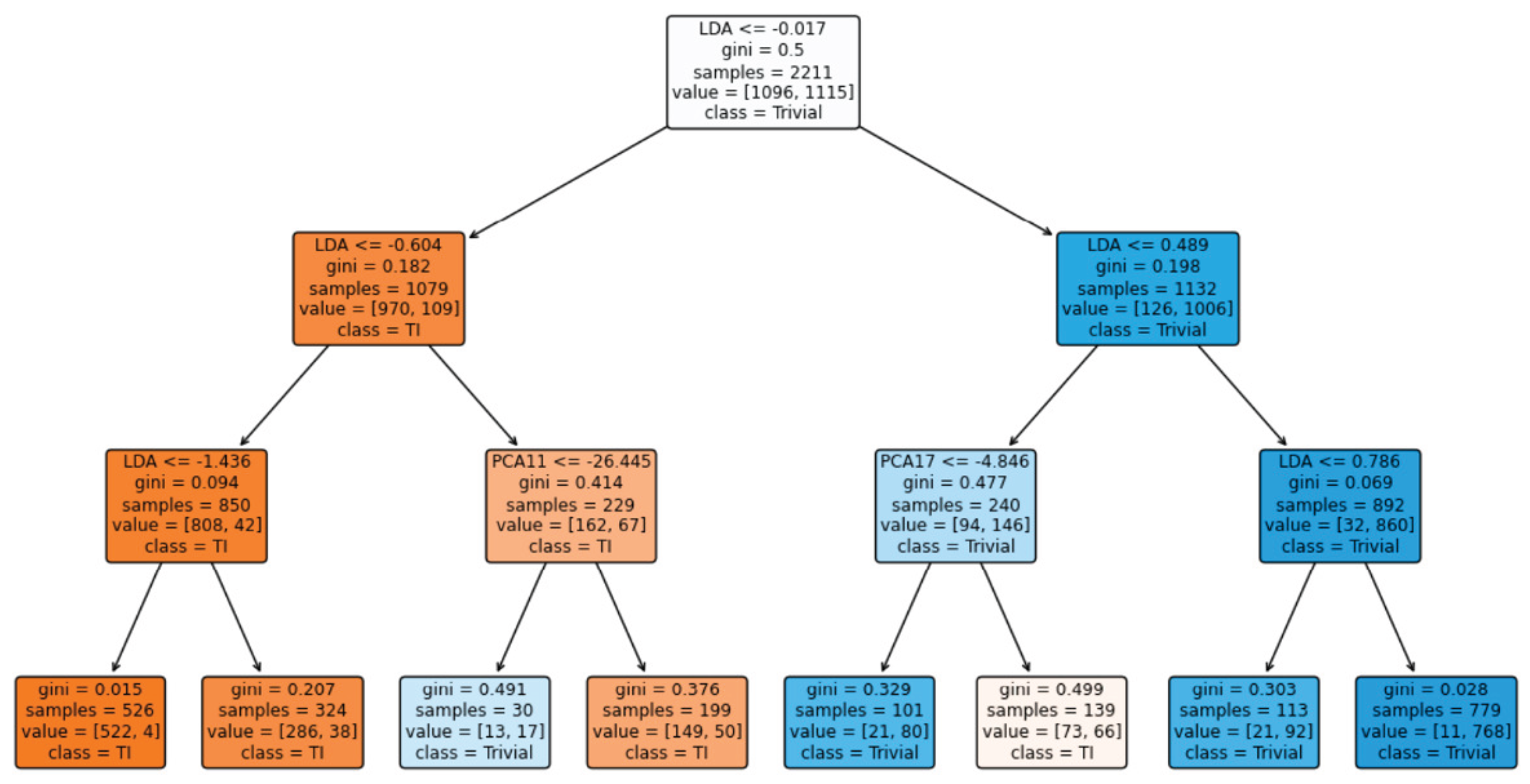

Table 1.
Metric values for each model built for the magnetic materials.
| Model | Accuracy | Precision | Recall | F1 Score |
|---|---|---|---|---|
| kNN | 0.766 | 0.730 | 0.836 | 0.780 |
| Bayesian | 0.774 | 0.870 | 0.639 | 0.737 |
| Decision Tree | 0.882 | 0.880 | 0.883 | 0.881 |
| SVM | 0.871 | 0.871 | 0.869 | 0.869 |
Table 2.
Metric values for each model built for the non-magnetic materials.
| Model | Accuracy | Precision | Recall | F1 Score |
|---|---|---|---|---|
| kNN | 0.941 | 0.797 | 0.787 | 0.792 |
| Bayesian | 0.915 | 0.707 | 0.690 | 0.699 |
| Decision Tree | 0.936 | 0.778 | 0.776 | 0.777 |
| SVM | 0.918 | 0.797 | 0.569 | 0.664 |
Disclaimer/Publisher’s Note: The statements, opinions and data contained in all publications are solely those of the individual author(s) and contributor(s) and not of MDPI and/or the editor(s). MDPI and/or the editor(s) disclaim responsibility for any injury to people or property resulting from any ideas, methods, instructions or products referred to in the content. |
© 2025 by the authors. Licensee MDPI, Basel, Switzerland. This article is an open access article distributed under the terms and conditions of the Creative Commons Attribution (CC BY) license (http://creativecommons.org/licenses/by/4.0/).
Copyright: This open access article is published under a Creative Commons CC BY 4.0 license, which permit the free download, distribution, and reuse, provided that the author and preprint are cited in any reuse.


