
Submitted:
14 October 2025
Posted:
15 October 2025
You are already at the latest version
Abstract
A two-dimensional computational fluid dynamics (CFD) analysis of a molten-salt natural circulation loop (MSNCL) was developed to investigate the flow and heat transfer behavior under buoyancy-driven conditions. Both laminar and Transition-SST models were employed in this study to observe how the two models interpret local phenomena inside an MSNCL system. The simulation results were validated against benchmark experimental data. Both models captured the overall temperature rise with increasing heater power, but the laminar model systematically underpredicted the flow velocity and Reynolds number due to its inability to represent turbulence-enhanced transport. This phenomenon is explained by examining the local distribution of velocity vectors and eddy-viscosity ratio and demonstrates the presence of secondary flow. The secondary local circulation appears to be stronger in the vertical leg as reported by several previous studies. Due to this condition, the Transition-SST model demonstrated superior capability in reproducing both global circulation and local flow phenomena compared to the laminar model. This study emphasizes the importance of turbulence modeling in accurately predicting molten-salt natural circulation behavior.
Keywords:
Molten salt
; Natural circulation loop
; CFD
; Heat and mass transfer
; Laminar
; Transient-SST
1. Introduction
As energy demand continues to grow, modern systems increasingly depend on technologies capable of storing and transferring heat efficiently. These requirements are especially critical in high-temperature applications such as concentrated solar power plants [1], advanced nuclear reactors [2,3], and various industrial processes such as heat treatment in the chemical industry [4,5]. In such systems, the choice of heat transfer fluid plays a decisive role, as it must operate safely at elevated temperatures, store large amounts of energy and maintain stability under low-pressure conditions [1]. Among the available options, molten salts have emerged as one of the most promising candidates, owing to their high boiling point, low vapor pressure, and excellent thermal stability, which together enable reliable operation at high temperatures without the need for pressurization [6]. Consequently, molten salts are now widely studied and applied as both coolants and thermal storage media across energy and industrial sectors.
Besides the excellent thermal properties, their use remains constrained by issues such as material corrosion and the risk of salt solidification under non-ideal operating conditions [7, 8]. These challenges increase system complexity and impose strict requirements on maintenance and start-up procedures. To minimize such operational risks, passive circulation concepts that can transport heat without mechanical pumping have gained significant interest. Natural circulation loops (NCLs) are particularly attractive because heat transfer is achieved solely through buoyancy forces, eliminating moving components and reducing both maintenance effort and failure probability. Building on this principle, several nuclear reactor development projects such as MASLWR [9], LFR [10], STAR-LM [11], ABV [12], and CAREM [13] have adopted single-phase natural circulation to remove heat from its core.
With their promising role in both energy production and storage, molten-salts have been extensively studied across a wide range of topics, including physical property characterization [14,15], corrosion and solidification behavior [7,8], forced convection heat transfer [16,17], and natural convection heat transfer [19,20,21,22,23,24,25,26]. Srivastava et al. [19] investigated the performance of molten-salt natural circulation loops (NCLs) under steady and transient conditions using different heating and cooling configurations, while Vijayan et al. [20] focused on flow stability and pressure-drop characteristics under varying heater-cooler placements. Karl et al. [21] examined a molten-salt mixture of LiF–BeF2 (FLiBe), highlighting its suitability for high-temperature operation above 700 °C compared to nitrate-based salts that remain stable only below 550 °C [22]. Jadyn et al. [23] employed particle image velocimetry (PIV) to visualize molten-salt flow behavior, revealing underdeveloped boundary layers and wall-peaked velocity profiles caused by high Prandtl number effects. From a modeling perspective, Vijayan et al. [24] and Gartia et al. [25] developed generalized scaling laws and correlations for predicting circulation Reynolds numbers in natural convection systems. Srivastava et al. [26] further coupled experimental studies with a one-dimensional numerical model (LeBENC code) originally developed by Borgohain [27] for water and lead–bismuth loops, showing good agreement with experimental results despite the assumption of incompressible flow and neglected viscous terms. Kudariyawar et al. [28] extended this approach using three-dimensional CFD modeling with a laminar formulation and the SIMPLE algorithm to study steady and transient molten-salt behavior.
Although both one-dimensional and three-dimensional studies have shown good agreement with experimental data, the local flow dynamics and turbulence development within molten-salt loops remain insufficiently explored. This limits the understanding of how buoyancy-driven instabilities evolve and influence overall circulation performance. In this study, a two-dimensional computational fluid dynamics (CFD) model of a molten-salt natural circulation loop is developed using both a laminar formulation and the Transition-SST turbulence model to capture coupled temperature and momentum transport. The two approaches are systematically compared with each other and validated against available experimental benchmark data under steady-state and transient conditions. The analysis includes temperature validation, transient temperature evolution with increasing heater power, and Reynolds number comparison to assess each model’s reliability. The results show that both models reproduce key experimental trends, but the Transition-SST model provides superior accuracy by capturing local circulation features and turbulence development within the loop. These insights enhance understanding of molten-salt natural circulation behavior and highlight the importance of turbulence modeling in predicting buoyancy-driven thermal systems.
2. Method: Experimental Benchmark
The validation of the present numerical work is carried out against the experimental results of Molten-Salt Natural Circulation Loop (MSNCL), which has been described in detail by Srivastava et al. [22]. A simplified schematic of the facility is shown in Figure 1. The loop is fabricated from Inconel 625 piping and arranged in a rectangular configuration with a height of approximately 2 m and width of 1.4 m. The pipe used in the experiment has a standard code of 15mm NB (1/2”) SCH 80 following the ANSI standard. The loop is supplied with molten salt that is initially melted in the Melt Tank and transferred into the main circuit by pressuring the Melt Tank with Argon gas. Once the loop is charged, natural circulation is established through the application of electrical heating in the heater section and forced air cooling in the cooler section.
The primary driving mechanism is buoyancy, where density differences between the heated and cooled sections induce continuous circulation of the molten salt. Temperature sensors are located at the inlet and outlet of both the heating and cooling sections, providing the bulk temperature data used for validation in this study. As molten salt undergoes thermal expansion and contraction during operation, an expansion tank is integrated at the top of the loop to maintain safe operating pressure and to accommodate volume fluctuations. The overall design ensures that stable natural circulation can be sustained under different heater–cooler configurations, while the present study specifically considers the vertical heater and vertical cooler (VHVC) arrangement. The design and preparation of the loop, including Argon purging, pressurization of the melting tank for initial salt charging, and emptying of the expansion tank, are explained in detail by Srivastava et al. [22]. In the present study, these steps are only summarized and referenced, as the focus remains on the benchmark temperature and velocity data.
3. Numerical Method
3.1. Governing Equation
The molten salt flow is modeled as a single-phase, incompressible fluid with heat transfer, governed by the conservation of mass, momentum, and energy. In natural circulation, buoyancy forces generated by temperature-dependent density variations drive the flow. The Boussinesq approximation is applied, treating density as constant except in the gravity term, where it varies linearly with temperature (Eq. 1). A similar approach for natural circulation modeling also reported by Kudariyawar et al. [24].
The flow field was solved using either a laminar or Transition-SST turbulence model to represent momentum transport. Both models assume a single-phase, incompressible, Newtonian fluid, with incompressibility defined in Eq. (2).
The momentum equations for the laminar model are given in Eqs. (3) and (4) for the x and y directions, respectively. The left-hand side represents unsteady and convective momentum transport, while the right-hand side includes pressure gradient and viscous diffusion terms. In the y-direction, a buoyancy term is added via the Boussinesq approximation of Eq. (1), where temperature-dependent density variations generate the driving force for natural circulation.
The Transition–SST model was employed to represent the laminar-to-turbulent transition in the molten salt natural circulation loop. Natural circulation flows are typically transitional, exhibiting laminar recirculation zones alongside turbulent mixing regions. Unlike fully turbulent models such as the standard k–ε or k–ω, which, if applied to low-Reynolds-number natural convection, tend to overpredict eddy viscosity. The Transition–SST model introduces additional transport equations for intermittency (γ) and the transition momentum-thickness Reynolds number (Reθ) to control turbulence onset and growth. This formulation allows the flow to remain laminar until local transition criteria are met, providing a more realistic description of buoyancy-driven flow behavior. The turbulent modification to the momentum equation is introduced through the effective viscosity term, as shown in Eq. (5).
In the Transition–SST model, four additional transport equations are solved for turbulent kinetic energy (k), specific dissipation rate (ω), intermittency (γ), and transition momentum-thickness Reynolds number (Reθ). These equations are shown in Eq. (6), (7), (8), and (9) respectively. The transition Reynolds number equation provides a local estimate of the critical Reθ for transition onset, which is then used as input to the intermittency equation. The intermittency field governs whether turbulence production is suppressed or activated: in laminar regions γ≈0, and turbulence production in the k-equation is damped, while in transitional and turbulent regions γ rises toward unity, allowing turbulence production to proceed. The k and ω equations then determine the turbulence kinetic energy and timescale, from which the eddy-viscosity μt is calculated. This turbulent viscosity is finally introduced into the momentum and energy equations as an effective transport property, thereby closing the RANS system and allowing laminar, transitional, and turbulent zones to be represented consistently within a single framework.
The energy equation includes unsteady, convective, and diffusive term. In the turbulent model, the same formulation is used but with an effective thermal conductivity that incorporates eddy-viscosity and the turbulent Prandtl number, accounting for enhanced energy transport by turbulence.
3.2. Geometry and Mesh
A two-dimensional model of the Molten Salt Natural Circulation Loop (MSNCL) was developed based on the experimental setup of Srivastava et al. [22], which serves as the validation reference. The geometry represents a rounded rectangular loop comprising vertical riser and downcomer sections connected by horizontal arms and curved bends. The loop height and width are 2000 mm and 1400 mm, respectively, with bends of 38 mm centerline radius following ANSI standards for NSP 1/2” piping. Minor structural details such as fittings and ports were omitted, as they have negligible influence on overall flow behavior. This geometric simplification aligns with prior numerical studies aimed at capturing the dominant hydrodynamic characteristics rather than precise construction details.
Mesh verification was performed using the Grid Convergence Index (GCI) method to quantify discretization error and confirm grid independence. The mesh was characterized by three parameters: normal cell size, first-layer thickness, and total element count. Coarser and finer grids were generated using a fixed refinement ratio to evaluate convergence of key outputs such as velocity and temperature. Inflation layers were added near the walls to capture velocity and temperature gradients accurately. For the Transition–SST model, the first layer was adjusted to keep y+ close to 1 and below 5, ensuring accurate near-wall resolution without using wall functions [27]. Mesh parameters for each refinement level are listed in Table 1, and the final mesh layout is shown in Figure 2.
3.3. Material, Boundary and Initial Condition
The working fluid is a 60:40 wt% mixture of sodium nitrate (NaNO3) and potassium nitrate (KNO3), whose thermophysical properties have been reported as temperature-dependent functions in the literature [28]. This approach follows previous 1-D [22] and 3-D [24] modeling studies, ensuring consistency with the simulation environment. Details of the polynomial constants used to calculate the thermophysical properties of the salt are shown in Table 2. It is important to note that the property correlations have been converted to accommodate temperature input in Kelvin rather than Celsius, as presented in the original source. The loop material is Inconel 625, with properties taken from [29].
Boundary conditions are specified separately for momentum and energy transport. For momentum, all internal walls are assigned a no-slip condition, enforcing zero velocity at the solid boundaries. As the loop is closed, no inlet or outlet conditions are defined; circulation is driven solely by buoyancy forces. Gravity is applied in the vertical direction with an acceleration of g = – 9.81 m/s2, acting downward. For energy boundary conditions, the molten salt operates between 200 and 500 °C (~473–773 K), consistent with the benchmark experiment. The heating section is modeled with a uniform heat flux corresponding to input powers of 1500–2000 W, while the cooling section is set as an isothermal wall at 200–220 °C (~473–493 K) to represent forced air cooling. All remaining loop walls are treated as adiabatic with zero heat flux.
The initial condition for the simulation assumes the molten salt is at rest throughout the loop (u=v=0) and uniformly set to an initial temperature of 300 °C (573.15 K). The pressure field was initialized with an equilibrium gauge pressure of 0 Pa, providing a neutral reference for the entire domain. The turbulence variables required for the Transition–SST model (k, ω, γ, and Reθ) were initialized using the default settings in ANSYS Fluent, with γ set to zero in the domain to represent fully laminar initial conditions. During the iterations, these fields developed consistently with the applied boundary conditions and the transition model correlations.
3.4. Modeling Approach and Numerical Scheme
The simulations were performed in transient mode using the pressure-based solver in ANSYS Fluent. The governing equations are the incompressible Navier–Stokes equations with gravity included in the vertical direction (y-axis) to represent buoyancy forces. Pressure–velocity coupling is handled with the SIMPLE algorithm, while the transient formulation employs a first-order implicit scheme to ensure numerical stability. Spatial discretization is performed with second-order schemes for convection and diffusion terms.
Convergence criteria are set to residuals of 10-4 for continuity and velocity, and 10−7 for energy. The turbulence transport equations— k, ω, intermittency and transition Reynolds number are maintained at their default Fluent thresholds of 10−3. The convergence behavior indicates stable computation, with fewer than 50 iterations required per time step during the initial transient phase. As the system approaches a quasi-steady circulation state, where temperature and velocity variations become less pronounced, the required iterations decrease to 3–4 per time step. This occurs after approximately 2000-3000 s of simulated physical time.
All simulations were performed on an AMD Ryzen Threadripper 1950X workstation with a maximum capacity of 32 cores. Parallel computing was performed on 16 cores to balance efficiency and resource allocation. Each simulation case required between 6 and 12 hours of computation time.
4. Results and Discussion
4.1. Mesh Verification
Table. 3 summarizes the results of the mesh independence study conducted for both the laminar and Transition-SST models, using three successively refined meshes (coarse, medium, and fine). The parameters evaluated were the average loop temperature (Tavg) and the heater–cooler section velocity (uHC). For both models, the Grid Convergence Index (GCI) values between the successive mesh levels (GCI3−2, GCI2−1) were found to be below 1%, indicating that the numerical solutions are mesh-independent within acceptable uncertainty. The asymptotic range values, all close to unity, confirm that the solutions lie within the asymptotic convergence region.

Table 3.
Summary of mesh-study results.
| Model | Asymp. Range | |||||||
|---|---|---|---|---|---|---|---|---|
| Transient-SST | 323.67 | 321.05 | 320.69 | 7.95 | 0.15 | 0.02 | 0.992 | |
| Transient-SST | 0.0799 | 0.0796 | 0.0794 | 2.11 | 0.47 | 0.23 | 0.996 | |
| Laminar | 329.15 | 327.63 | 328.17 | 2.82 | 0.32 | 0.11 | 0.995 | |
| Laminar | 0.0726 | 0.0728 | 0.0740 | 0.16 | 0.40 | 2.52 | 1.003 |
For the Transition-SST model, Tavg converged from 323.7 K to 320.7 K with a GCI of 0.02%, while uHC showed minor variation with a maximum GCI of 0.23%. Similarly, the laminar model exhibited stable convergence, with Tavg decreasing slightly from 329.1 K to 328.2 K and a GCI below 0.11%. Considering the GCI was evaluated with a 95% confidence level (using a safety factor of 1.25), these small GCI values confirm grid-independent solutions. The close agreement among grid levels confirms that numerical errors from spatial discretization are negligible, and that the remaining differences between the laminar and Transition–SST models originate from turbulence modeling.
4.2. Steady-State and Transient Modeling
Figure 3a presents the comparison of outlet (THO) and inlet (THI) temperatures between experimental measurements and CFD predictions under steady-state conditions. Both the laminar and Transition–SST simulations reproduce the experimental temperature trends with only minor deviations, indicating that the developed model accurately reflects the heat transfer and circulation characteristics of the loop. The temperature range obtained in this study falls within the stable operating regime of nitrate-salt natural circulation reported in Refs. [22, 24]. The data for steady-state analysis were taken after the system had achieved dynamic equilibrium, as indicated by the stabilization of both the heater temperature and the loop’s average temperature.
Figure 3b. compares the transient temperature response of the loop between experimental measurements and CFD predictions obtained using the laminar and Transition–SST models. The simulation was conducted under a stepwise heating input, initially operated at 1500 W for 10,000 s to ensure steady-state convergence, followed by an increase to 1600 W for another 10,000 s. This setup allows the evaluation of how the system temperature evolves over time as it transitions toward a new equilibrium condition. Both models successfully reproduce the experimentally observed temperature rise, accurately capturing the gradual response of the molten nitrate salt as the loop adjusts to the higher power level. The predicted outlet temperature (THO) increases smoothly and stabilizes after approximately 3000–4000 s, indicating that the simulation correctly represents the transient heat accumulation and circulation dynamics. While the Transition–SST model shows slightly faster recovery during the early phase and have closer range to experimental result, the overall deviation between the two models remains within 5%, which falls in a reasonable range of experimental uncertainty. This result implies that, under the present conditions, both flow regimes provide physically consistent predictions, and the observed agreement confirms that the numerical framework can reliably simulate the transient thermal response of the natural circulation loop.
4.3. Reynolds Number Validation
Figure 4 presents the variation of the loop Reynolds number with heater power, comparing CFD predictions with experimental data. The experimental Reynolds number increases steadily with power, reflecting higher buoyancy-driven flow velocity as thermal input increases. Both CFD models reproduce the upward trend, but with different levels of accuracy.
The laminar model systematically underpredicts the Reynolds number across the entire power range, falling outside the 10% error bars of experimental data. This underestimation arises from the absence of turbulent transport mechanisms, which in reality enhance momentum transfer and sustain higher bulk velocities. In contrast, the Transition-SST model shows much closer agreement with the measurements, showing deviations generally within the ±10% error band. The improved performance of the turbulence model highlights its ability to capture the flow dynamics of natural circulation loop of molten salt.
The proposed explanation for the difference between the two models lies in how each interprets the local flow dynamics within the loop. The bulk momentum driving circulation originates from the temperature difference between the heating and cooling sections, but additional temperature gradients also develop locally along the loop walls. These local variations influence buoyancy and viscosity, thereby shaping the detailed flow distribution. A previous study by Jadyn et al. [23] reported the presence of near wall velocity peaks in the heater section, attributed to the high Prandtl number of molten salts creating an incomplete development of thermal boundary layer. The further effect of the under developed thermal boundary layer is a secondary circulation exist locally especially at the vertical leg where the flow direction is on the same axis with gravity.
4.4. Local Velocity Distribution
Figure 5 compares the axial velocity distributions at the heater and cooler sections of the loop for both laminar and Transition-SST models. In the heater section, the velocity profile exhibits a distinct M-shaped structure with velocity peak near heater wall as the temperature is highest. This is confirming with the founding of Jadyn et al [23] regarding the under developed thermal boundary layer at heating section of molten-salt natural circulation loop. This behavior arises from buoyancy-driven acceleration of fluid adjacent to the hot surfaces, where heated fluid rises more vigorously and forms wall-driven jets, while the core region responds more slowly.
In contrast, the cooler section exhibits a velocity distribution similar to that of a classical fully developed laminar flow, characterized by a single centerline peak and a smooth decay toward the walls. This behavior arises because cooling increases the local fluid density, which decelerates the near-wall flow, while the relatively warmer fluid near the center maintains higher velocity, producing the parabolic profile typical of laminar flow.
These results highlight a distinct asymmetry in the velocity regimes between the heated and cooled sections of the loop: heating destabilizes the velocity field through strong wall-driven acceleration, whereas cooling promotes flow stabilization and re-laminarization. This contrast underscores the importance of appropriate turbulence modeling for accurately capturing local transport phenomena in buoyancy-dominated natural circulation loops.
Figure 6.
Velocity Contour of MSNCL – Comparing Laminar and Transition-SST models.
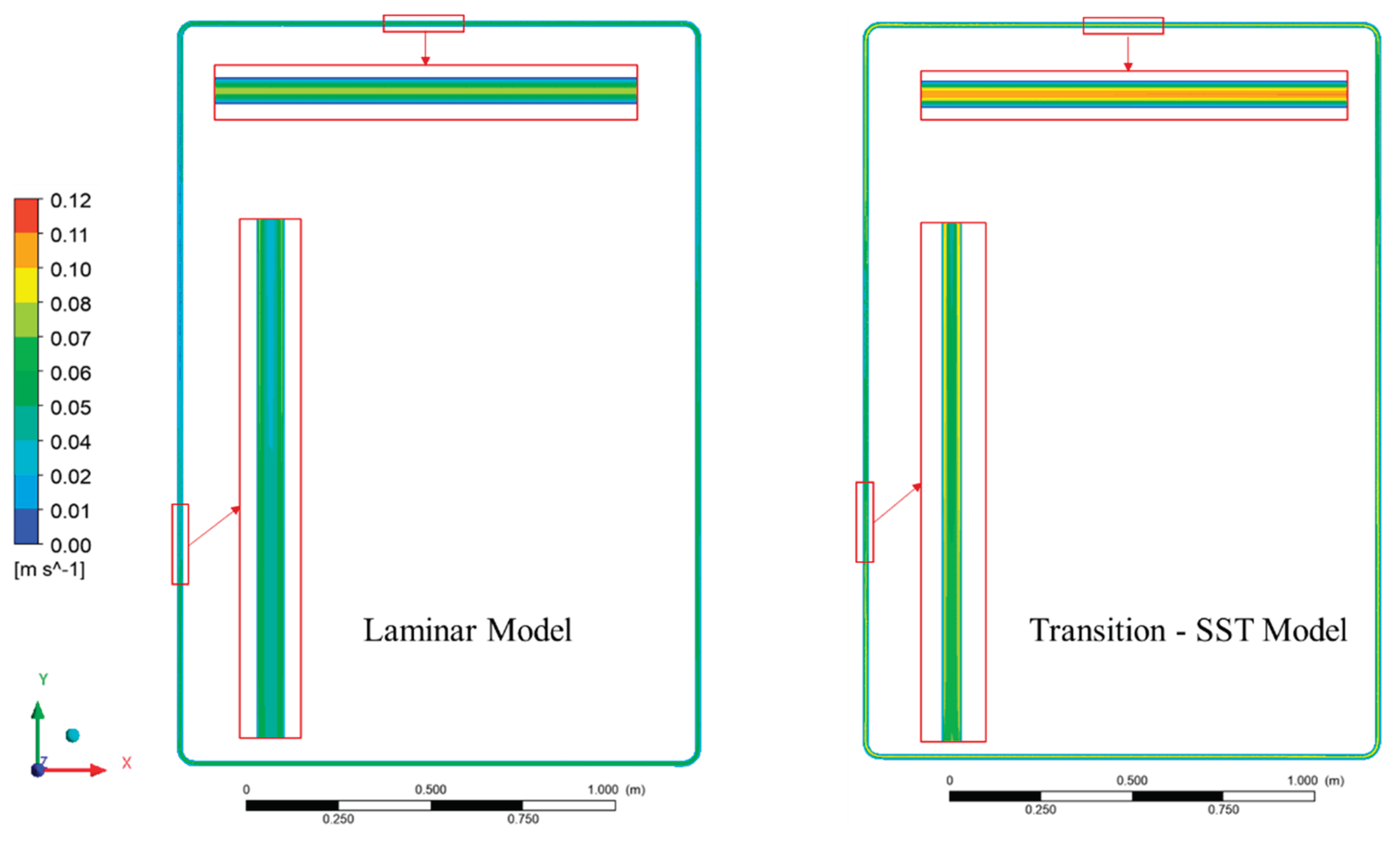
Figure 7 also presents velocity distribution but in a graphical form. The color contours indicate that the Transition-SST predicts higher velocity magnitude compared to the laminar model. It also depicts how the distribution of velocity locally along the loop geometry. Taken together, the contour visualization provides a clear graphical confirmation of the velocity profile analysis: heating promotes wall peak velocity formation and transitional turbulence, while cooling stabilizes the flow and restores a laminar-like parabolic profile. The closer agreement of the Transition-SST predictions with experimental Reynolds numbers (Figure 5) further supports the physical realism of the turbulence model in capturing local flow features in natural circulation loops.
4.5. Local Circulation Modeling on Laminar and Transition-SST
Local circulation effects are particularly pronounced in the vertical leg of the loop, where buoyancy forces are directly opposed by gravitational stratification. From a dimensional perspective, the strength of natural circulation can be characterized by the Rayleigh number, in which the characteristic length appears as a cubic term. This strong dependence implies that even modest changes in local flow geometry or thermal gradients can significantly amplify circulation asymmetries and promote recirculation zones. In the present study, the transient SST model enables these effects to be observed more clearly through the use of turbulence-related parameters. Specifically, the eddy-viscosity ratio is employed to identify regions of enhanced turbulent transport, while the laminar model provides complementary visualization of circulation patterns through normalized velocity vectors and contours (Figure 8).
Figure 6.
Observation of the local circulation presence – From both laminar model and Transient SST model’s perspective.
Figure 6.
Observation of the local circulation presence – From both laminar model and Transient SST model’s perspective.
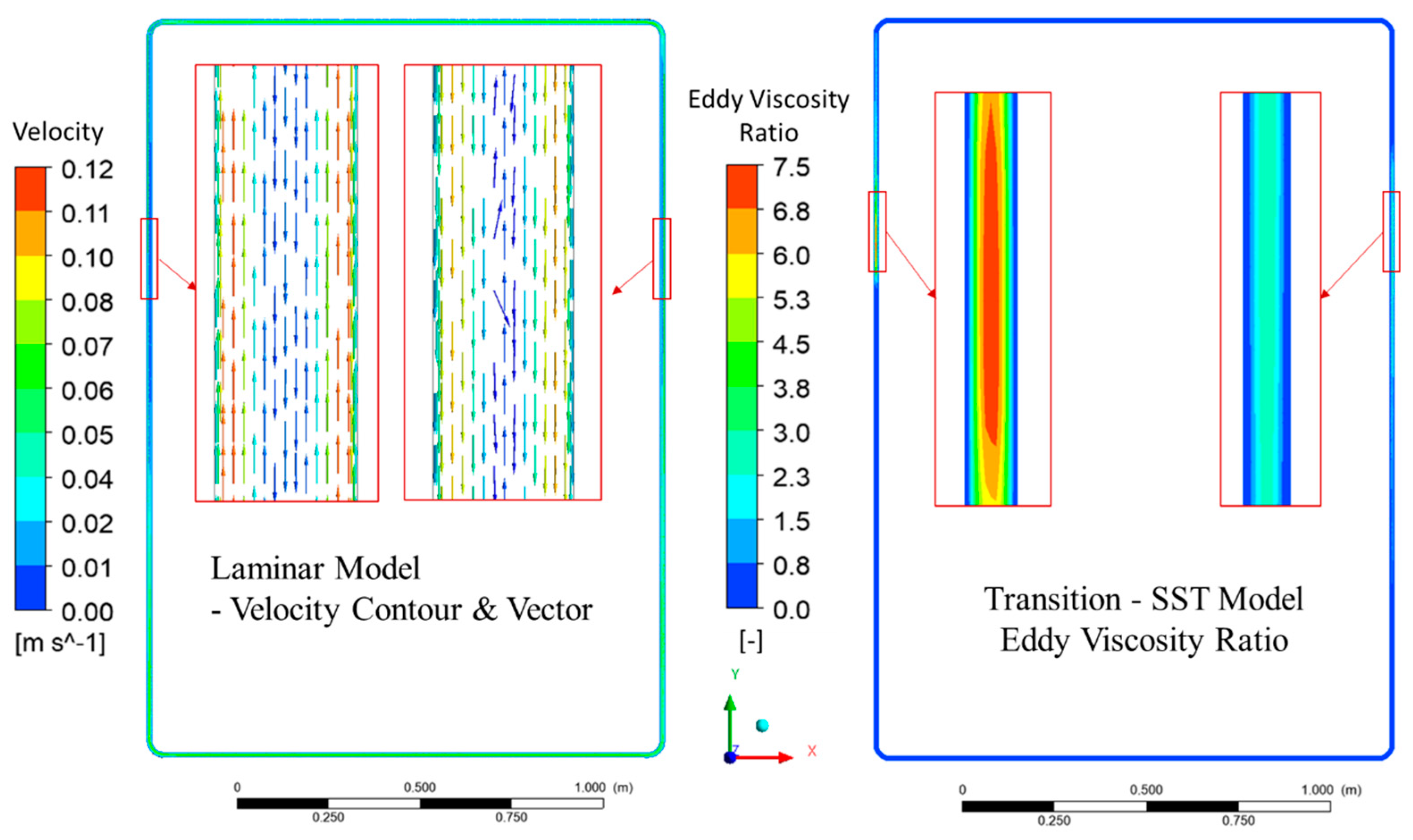
In the laminar case, velocity vectors were normalized to emphasize flow directionality rather than absolute magnitude. This representation highlights the tendency of the core flow near the channel centerline to approach zero velocity at the outlet, which the solver perceives as a weak reverse flow. Such localized recirculation contributes to an overall damping of the mean velocity in the loop, thereby leading the laminar model to systematically underpredict the Reynolds number when compared against experimental benchmarks. In contrast, the Transition-SST model captures the emergence of turbulent transport via elevated eddy-viscosity ratios in the same vertical leg region, which prevents excessive damping and yields velocity fields that are more consistent with experimental trends.
4.6. Turbulence Magnitude and Heating Power
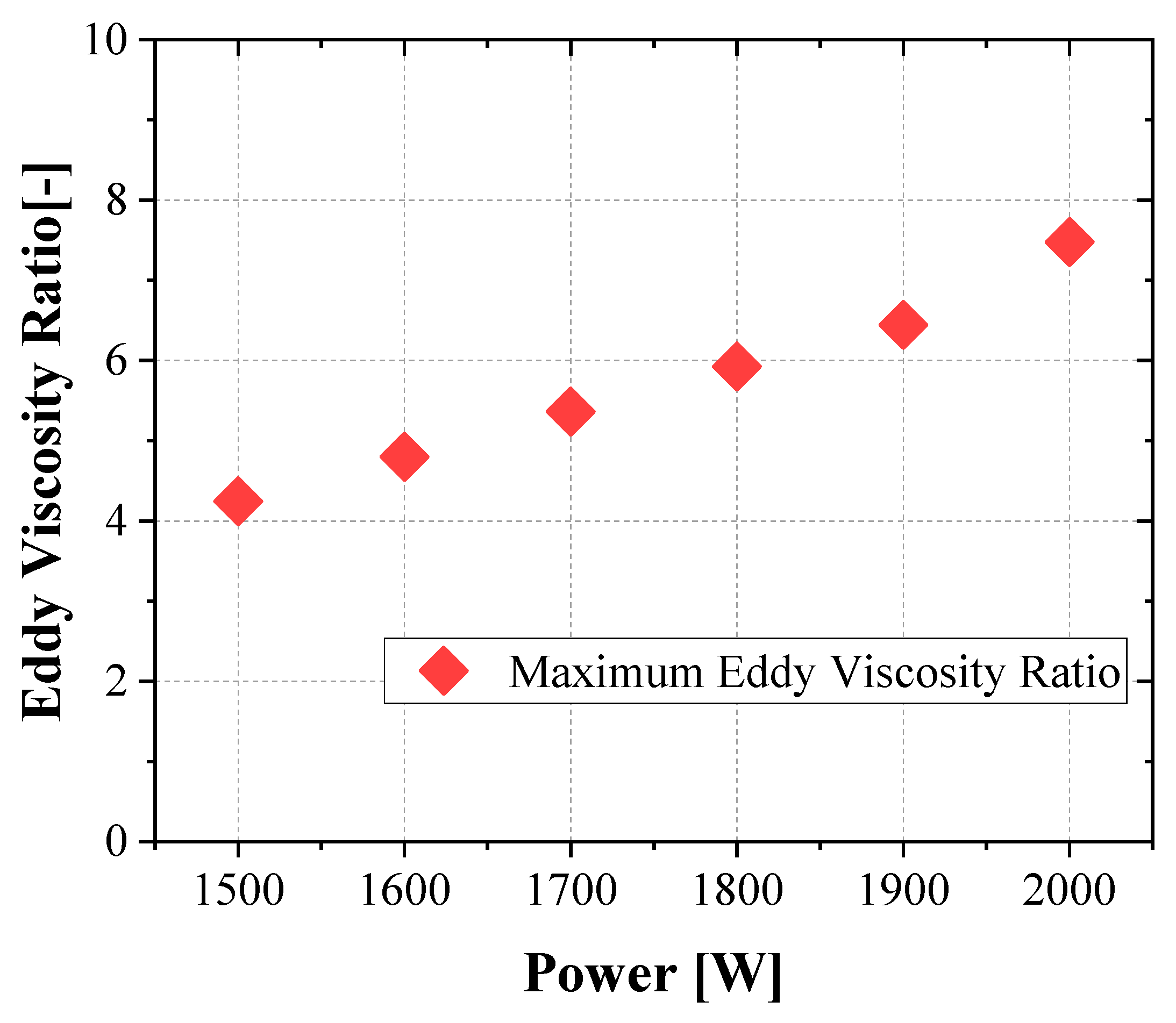
The measure of turbulence magnitude under different heating power is demonstrated using eddy viscosity ratio. Figure 9 presents the variation of the maximum eddy-viscosity ratio (μt/μ) in the loop as a function of heating power. The eddy-viscosity ratio is a turbulence modeling parameter that quantifies the relative strength of turbulence-induced momentum transport compared to molecular viscosity. In this study, the maximum value within the domain is extracted at each power level to provide an insight how the value changes as the heat is increases.
As shown in the figure, the maximum eddy-viscosity ratio increases steadily with heating power. At lower power inputs, the ratio remains relatively modest, indicating that buoyancy-driven circulation is predominantly laminar with only weak turbulent contributions. With increasing power, however, the buoyancy forces intensify, leading to larger velocity gradients and stronger thermal stratification, particularly in the vertical leg. This phenomenon explains why the range of error for prediction increases as the heating power is increase (Figure 5). This trend demonstrates that the eddy-viscosity ratio is a meaningful parameter to diagnose turbulence development in natural circulation loops. While the Reynolds number provides a global measure of the overall circulation strength, the eddy-viscosity ratio highlights localized enhancement of turbulent transport. Although further study is needed, the observed rise in turbulence with increasing heating power indicates that the loop may approach a stability limit. Beyond this limit, stronger buoyancy forces could cause unsteady or oscillatory flow behavior, as noted in earlier studies [22, 24].
Figure 6.
Variation of the maximum eddy-viscosity ratio with heater power in the MSNCL.
5. Conclusions
A two-dimensional CFD study of a molten-salt natural circulation loop was performed and compared with published experimental benchmark data. Both laminar and Transition-SST turbulence models were evaluated to assess their ability to reproduce global and local flow behavior. The key conclusions from this study are outlined below.
- The two employed models were verified numerically using the Grid Convergence Index to assess its grid independence.
- The predicted temperature difference across the loop showed good agreement with experimental data for both laminar and Transition-SST models, falling within the acceptable range of variation.
- The laminar model underpredicted bulk velocity, while the Transition-SST model reproduced the experimental Reynolds number more accurately. This is due to the Transition-SST model successfully resolves local circulation and eddy-viscosity development, whereas the laminar model misinterprets the same phenomena as backflow, causing reduced global circulation strength.
- Velocity vector plots indicated stronger recirculation zones in the laminar case. These structures are consistent with the presence of turbulent transport, which in the Transition-SST model manifests as finite eddy-viscosity. The agreement between local flow patterns and the eddy-viscosity distribution supports the physical realism of the Transition-SST results.
- The increasing eddy-viscosity ratio with power confirmed the progressive transition from laminar to transitional–turbulent flow regimes, underscoring the importance of turbulence modeling for accurate prediction of Natural Circulation Loop.
Author Contributions
Conceptualization, B.F.S and J.Y.L; methodology, B.F.S and J.Y.L; software, B.F.S; validation, B.F.S; formal analysis, B.F.S; investigation, B.F.S; resources, J.Y.L; data curation, B.F.S; writing—original draft preparation, B.F.S; writing—review and editing B.F.S and J.Y.L; visualization, B.F.S; supervision, J.Y.L; project administration, J.Y.L; funding acquisition, J.Y.L; All authors have read and agreed to the published version of the manuscript.
Funding
This work was supported by Korea Hydro & Nuclear Power Co and Local Government (Pohang). (2025).
Conflicts of Interest
The authors declare no conflicts of interest.
Nomenclature
| Cartesian coordinate | Field variable (for mesh study) | ||
| Velocity component of x and y | Scalar value of | ||
| Time | |||
| Density | Subscripts | ||
| Pressure | eff | Effective property | |
| Viscosity | t | Turbulent quantity | |
| Gravity acceleration | HI | Heater inlet | |
| Thermal expansion coefficient | HO | Heater outlet | |
| Temperature | HC | Heater center | |
| Thermal conductivity | avg | Average | |
| Prandtl number | 0 | Reference point | |
| Production Term | |||
| Dissipation term | |||
| Transition model destruction term | |||
References
- Vignarooban, K. , et al. "Heat transfer fluids for concentrating solar power systems–a review." Applied Energy 146 (2015): 383-396.
- Roper, Robin, et al. "Molten salt for advanced energy applications: A review." Annals of Nuclear Energy 169 (2022): 108924.
- Forsberg, Charles W., Per F. Peterson, and Paul S. Pickard. "Molten-salt-cooled advanced high-temperature reactor for production of hydrogen and electricity." Nuclear Technology 144.3 (2003): 289-302.
- de Figueiredo Luiz, Debora, et al. "Review of the molten salt technology and assessment of its potential to achieve an energy efficient heat management in a decarbonized chemical industry." Chemical Engineering Journal 498 (2024): 155819.
- Shen, Yafei, and Xiangzhou Yuan. "Research advancement in molten salt-mediated thermochemical upcycling of biomass waste." Green Chemistry 25.6 (2023): 2087-2108.
- Williams, D. F. Assessment of candidate molten salt coolants for the NGNP/NHI heat-transfer loop. No. ORNL/TM-2006/69. Oak Ridge National Lab.(ORNL), Oak Ridge, TN (United States), 2006.
- Wei, Ying, et al. "Review of Molten Salt Corrosion in Stainless Steels and Superalloys." Crystals 15.3 (2025): 237.
- Lu, Jianfeng, Jing Ding, and Jianping Yang. "Solidification and melting behaviors and characteristics of molten salt in cold filling pipe." International Journal of Heat and Mass Transfer 53.9-10 (2010): 1628-1635.
- Reyes, Jose N., et al. "Testing of the multi-application small light water reactor (MASLWR) passive safety systems." Nuclear Engineering and Design 237.18 (2007): 1999-2005.
- Alemberti, Alessandro, et al. "Overview of lead-cooled fast reactor activities." Progress in Nuclear Energy 77 (2014): 300-307.
- Sienicki, James J., and Bruce W. Spencer. "Power optimization in the STAR-LM modular natural convection reactor system." International Conference on Nuclear Engineering. Vol. 35960. 2002.
- V.I. Kostin, O.B. V.I. Kostin, O.B. Samoilov, V.N. Valvilkin, Yu.K. Panov, A.V. Kurachenkov, M.A. Bolshukhin, V.I. Alekeev, I.V. Shmelev, Yu.D. Baranaev, A.A. Pekanov, Small floating nuclear power plants with ABV reactors for electric power generation, heat production and seawater desalination, in: Fifteenth Annual Conference of Indian Nuclear Society, INSACNovember 15-17, 2004, Mumbai, India.
- R. Mazzi, CAREM: an innovative integrated PWR, in: 18th International Conference on Structural Mechanics in Reactor Technology (SMiRT-18), Beijing, China, August 7-12, 2005, SMiRT18-S01-2.
- Cornwell, K. "The thermal conductivity of molten salts." Journal of Physics D: Applied Physics 4.3 (1971): 441.
- Ferri, Roberta, Antonio Cammi, and Domenico Mazzei. "Molten salt mixture properties in RELAP5 code for thermodynamic solar applications." International Journal of Thermal Sciences 47.12 (2008): 1676-1687.
- Yu-ting, Wu, et al. "Convective heat transfer in the laminar–turbulent transition region with molten salt in a circular tube." Experimental Thermal and Fluid Science 33.7 (2009): 1128-1132.
- Bin, Liu, et al. "Turbulent convective heat transfer with molten salt in a circular pipe." International communications in heat and mass transfer 36.9 (2009): 912-916.
- Alstad, C. D. The Transient Behavior of Single-phase Natural Circulation Water Loop Systems. Vol. 5409. Argonne National Laboratory, 1954.
- Srivastava, A. K., N. Saikrishna, and N. K. Maheshwari. "Steady state performance of molten salt natural circulation loop with different orientations of heater and cooler." Applied Thermal Engineering 218 (2023): 119318.
- Britsch, Karl, et al. "Natural circulation FLiBe loop overview." International Journal of Heat and Mass Transfer 134 (2019): 970-983.
- Reis, Jadyn, Joseph Seo, and Yassin Hassan. "Molten salt flow visualization to characterize boundary layer behavior and heat transfer in a natural circulation loop." Physics of Fluids 36.3 (2024).
- Srivastava, A. K. , et al. "Experimental and theoretical studies on the natural circulation behavior of molten salt loop." Applied Thermal Engineering 98 (2016): 513-521.
- Borgohain, A. , et al. "Natural circulation studies in a lead bismuth eutectic loop." Progress in nuclear energy 53.4 (2011): 308-319.
- Kudariyawar, Jayaraj Yallappa, et al. "Computational and experimental investigation of steady state and transient characteristics of molten salt natural circulation loop." Applied Thermal Engineering 99 (2016): 560-571.
- Gartia, M. R., P. K. Vijayan, and D. S. Pilkhwal. "A generalized flow correlation for two-phase natural circulation loops." Nuclear Engineering and Design 236.17 (2006): 1800-1809.
- Vijayan, P. K. , and H. Austregesilo. "Scaling laws for single-phase natural circulation loops." Nuclear Engineering and Design 152.1-3 (1994): 331-347.
- Menter, Florian R., et al. "A correlation-based transition model using local variables—part I: model formulation." Journal of turbomachinery 128.3 (2006): 413-422.
- Nissen, Donald A. "Thermophysical properties of the equimolar mixture sodium nitrate-potassium nitrate from 300 to 600. degree. C." Journal of Chemical and Engineering Data 27.3 (1982): 269-273.
- Kaschnitz, E., L. Kaschnitz, and S. Heugenhauser. "Electrical resistivity measured by millisecond pulse heating in comparison with thermal conductivity of the superalloy Inconel 625 at elevated temperature." International Journal of Thermophysics 40.3 (2019): 27.
Figure 1.
Simplified schematics of MSNCL experiment [22].
Figure 1.
Simplified schematics of MSNCL experiment [22].
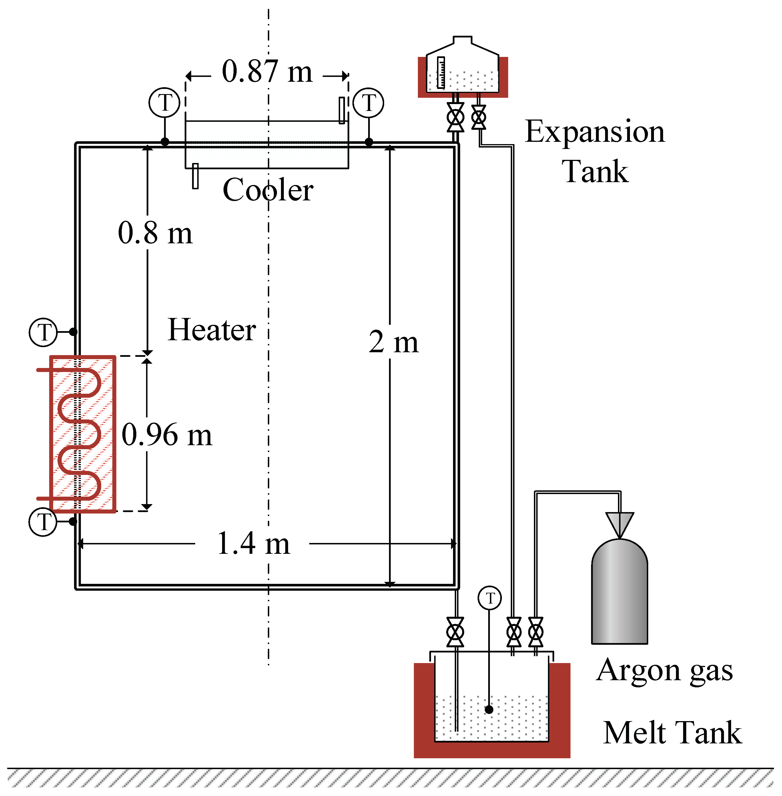
Figure 2.
Mesh structure of MSNCL.
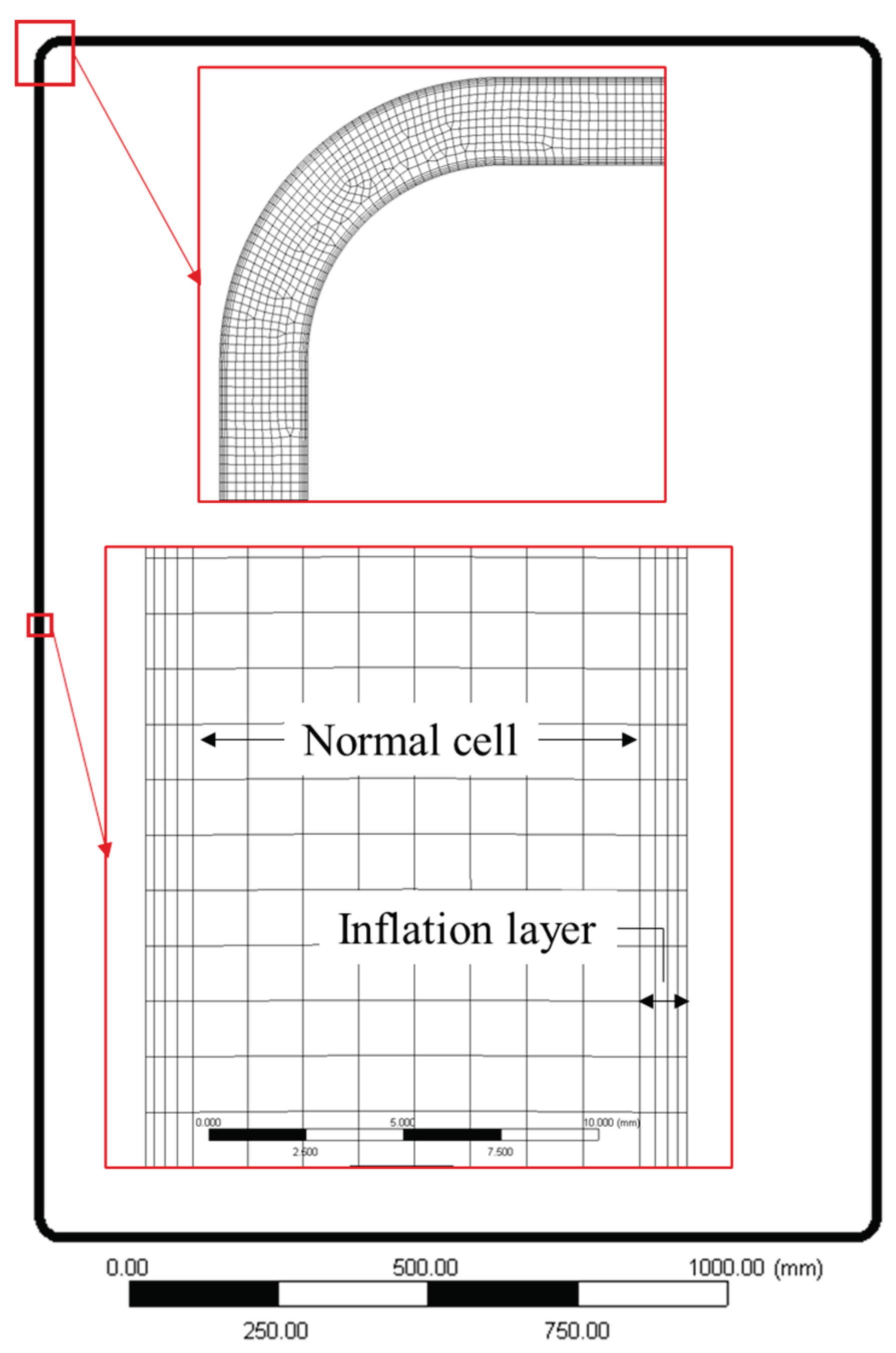
Figure 3.
Temperature validation for models against experimental data (a) Steady-state condition (b) Transient Condition.
Figure 3.
Temperature validation for models against experimental data (a) Steady-state condition (b) Transient Condition.
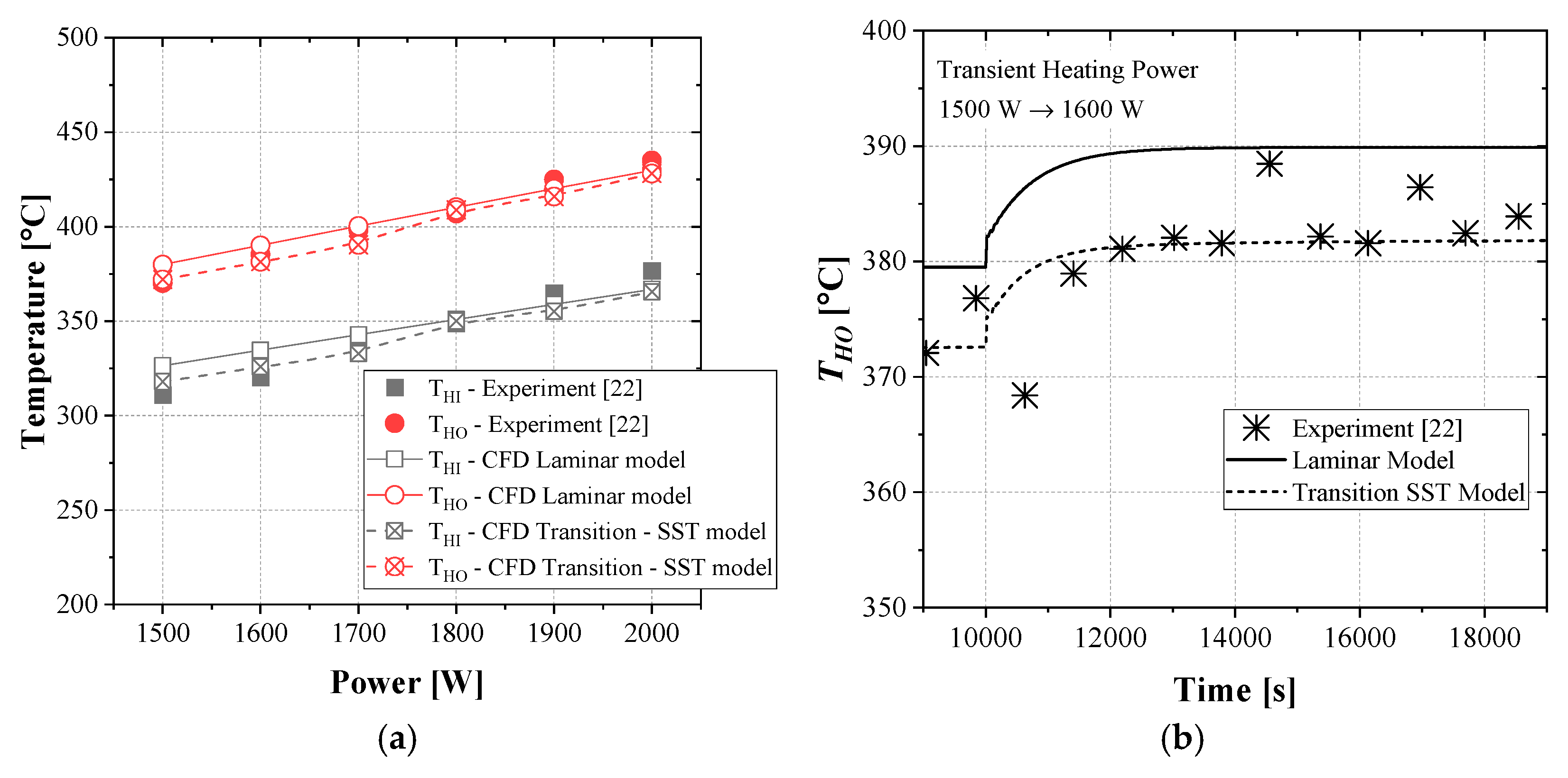
Figure 4.
Validation results of simulation models against benchmark experiment [22] – Reynolds number.
Figure 4.
Validation results of simulation models against benchmark experiment [22] – Reynolds number.
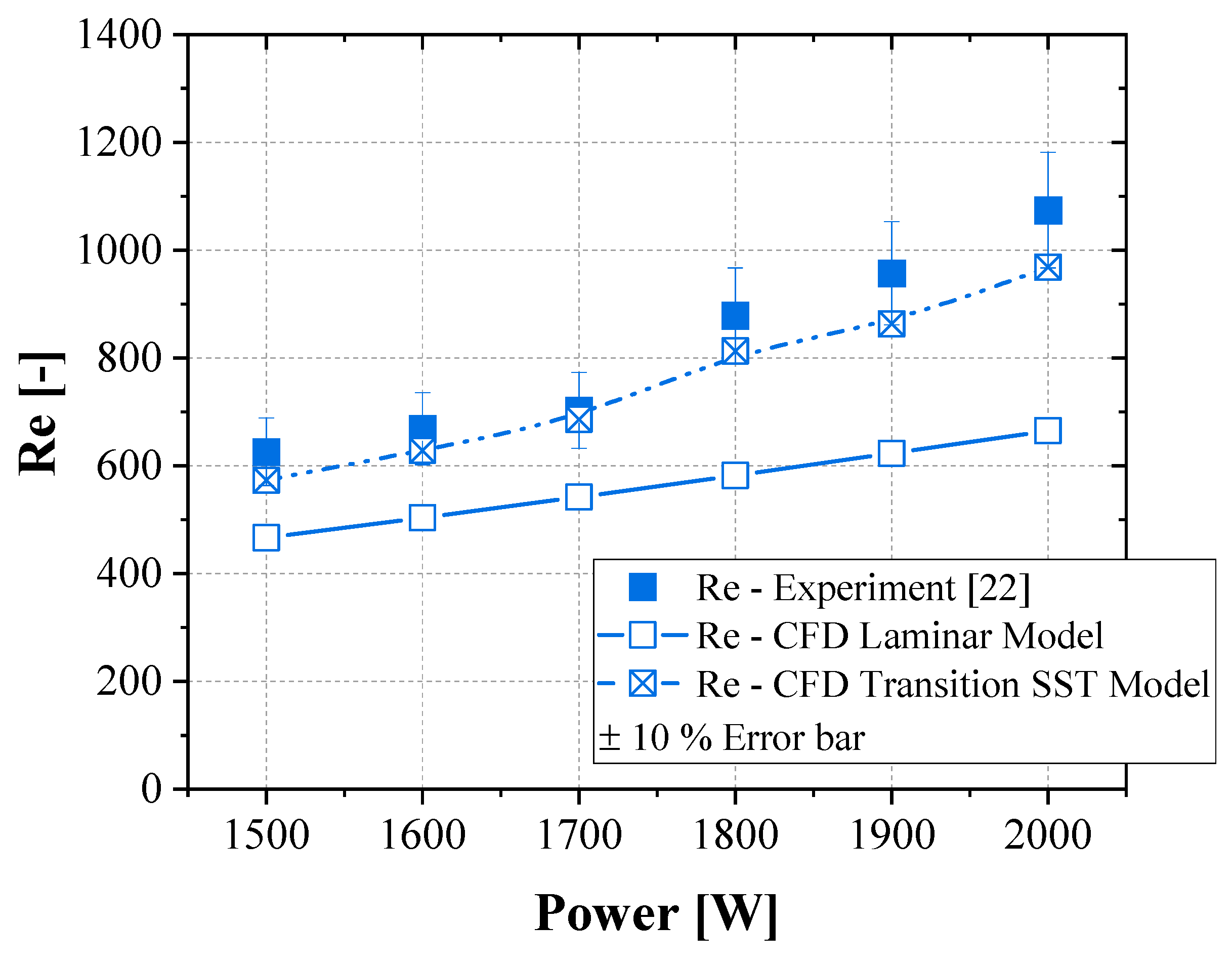
Figure 5.
Local velocity distribution on heating and cooling region (a) Laminar and (b) Transition-SST models.
Figure 5.
Local velocity distribution on heating and cooling region (a) Laminar and (b) Transition-SST models.
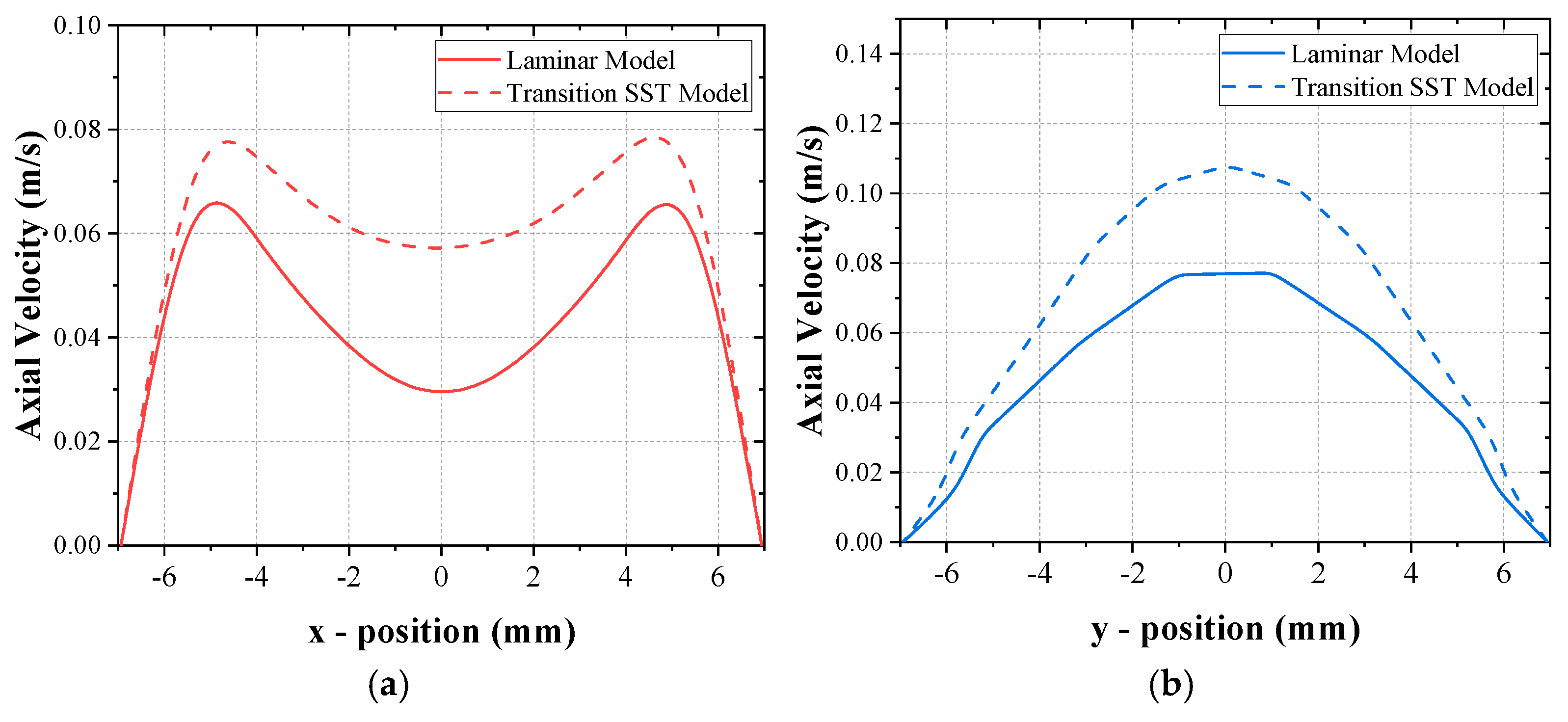
Table 1.
Summary of mesh configuration.
| #Mesh | Description | Normal Cell Size [mm] | First Layer Thickness [mm] |
Refinement factor [-] |
Maximum y+ [-] |
|---|---|---|---|---|---|
| 3 | Coarse | 2 | 0.31 | 1.3 | 2.45 |
| 2 | Medium | 1.4 | 0.22 | 1.3 | 1.7 |
| 1 | Fine | 1 | 0.16 | 1.3 | 1.2 |
Table 2.
Polynomial constant for temperature dependent properties of Nitrate salt [22, 24, 28].
| Parameter | a | b | c | d |
|---|---|---|---|---|
| 2263.723 | -0.636 | - | - | |
| 0.390 | 1.954 x 10⁻⁴ | - | - | |
| 1396.018 | 0.172 | - | - | |
| 7.551 x 10⁻² | -2.776 x 10⁻⁴ | 3.489 x 10⁻⁷ | -1.474 x 10⁻¹⁰ |
Disclaimer/Publisher’s Note: The statements, opinions and data contained in all publications are solely those of the individual author(s) and contributor(s) and not of MDPI and/or the editor(s). MDPI and/or the editor(s) disclaim responsibility for any injury to people or property resulting from any ideas, methods, instructions or products referred to in the content. |
© 2025 by the authors. Licensee MDPI, Basel, Switzerland. This article is an open access article distributed under the terms and conditions of the Creative Commons Attribution (CC BY) license (http://creativecommons.org/licenses/by/4.0/).
Copyright: This open access article is published under a Creative Commons CC BY 4.0 license, which permit the free download, distribution, and reuse, provided that the author and preprint are cited in any reuse.


