Submitted:
10 October 2025
Posted:
15 October 2025
You are already at the latest version
Abstract
A comprehensive study of the magnetic properties of baked clays containing ferrimagnetic particles in various magnetic states, including superparamagnetic, has been carried out in this work. The phase composition of the magnetic fraction of laboratory and industrial samples made from the same clay is mainly represented by iron (III) oxide polymorphs and possibly non-stoichiometric magnetite. Experimental methods included magnetic granulometry, Mössbauer spectroscopy, scanning electron microscopy, X-ray phase analysis, and pulsed electromagnetic measurements. A theoretical model of mag-netostatically interacting particles with a lognormal volume distribution was used to in-terpret the experimental data, allowing the contribution of superparamagnetic grains to be taken into consideration. It is shown that the firing mode significantly affects the composition of iron-oxide phases and their magnetic characteristics. Laboratory samples are characterized by approximately twice the proportion of superparamagnetic particles. At sufficiently low concentration of ferrimagnet in samples < 0.1 %, the concentration of superparamagnetic particles is even two orders of magnitude lower. It is the use of pulse methods that provides a more reliable diagnosis of their presence. The complex application of experimental methods with theoretical modeling makes it possible to reveal and quantitatively describe the microheterogeneous nature of the magnetic state of baked clays, which is applicable to a wide range of magnetic materials, and to analyze more deeply the thermal and phase history of archaeological and geological objects.
Keywords:
superparamagnetism
; polymorphs of iron oxides
; baked clays
; bricks
; blocking volume
; magnetostatic interaction
; magnetic susceptibility
; frequency dependence factor
; hysteresis characteristics
; magnetic granulometry
1. Introduction
Superparamagnetic nanoparticles of iron and its oxides represent an important object of research in geophysics, ecology, and materials science. They are widely distributed in soils, loesses, and sedimentary rocks, where they can serve as indicators of paleoecological conditions [1,2,3]. Fired clays are particularly relevant: their magnetic properties record the temperature history of thermal processes and can be used as “firing archives” [4,5]. Along with this, iron oxide nanoparticles are considered as a significant source of anthropogenic pollutants with potential effects on human health [6,7].
According to the classical concept of L. Néel [8], at a sufficiently small volume of a ferromagnetic particle or at elevated temperature, thermal fluctuations are able to overcome the energy barrier between states with opposite orientations of the magnetic moment. In this case, the momentum makes spontaneous reorientations, and the particle behaves as a superparamagnetic particle. The key parameter is the blocking volume vb, which sets the boundary between the blocked and superparamagnetic states. The blocking volume is defined as: , where is the measurement time; is the temperature at which the measurements are carried out; is the spontaneous magnetization; is the intrinsic magnetization reversal field (microcoercivity); is the Boltzmann constant; is the frequency factor.
For an ensemble of SP particles in a zero field, the average magnetization is zero, but an average moment directed along the field appears in an external field. The shape of the magnetization curves and the size of the blocking volume are significantly affected by interparticle interactions that change the distribution of relaxation times [9,10]. These effects lead to the appearance of magnetic viscosity and can contribute to the remanent magnetization.
The presence of superparamagnetic particles in soils and rocks can affect the results of geophysical surveys by the transient electromagnetic method (TEM soundings) [11]. It is known that transient processes distorted by the influence of superparamagnetism are characterized by the t–1 law, which is much slower than the decline of purely inductive response [12,13]. It has been shown that the use of electromagnetic sounding equipment in some cases allows detecting processes related to magnetic viscosity in field conditions [14,15,16], including archaeological studies [11,17,18]. Thus, the TEM method can be considered as one of the ways to study magnetic viscosity in the conditions of natural occurrence of rocks.
In baked clays, magnetic properties are controlled by phase transformations of iron-bearing minerals during heating. As the temperature increases, hydroxides (e.g., goethite, lepidocrocite) dehydrate and transform into maghemite and magnetite, while further heating produces hematite or metastable phases such as ε-Fe2O3 [19,20]. These transformations control the balance between superparamagnetic and ferrimagnetic grains.
Of particular interest are polymorphic modifications of iron oxides formed by thermal action on clays. The most common phases — magnetite (Fe3O4), maghemite (γ-Fe2O3), and hematite (α-Fe2O3) — have different magnetic properties and thermal stability. At the same time, metastable modifications, such as ε-Fe2O3 and β-Fe2O3, are often formed by rapid heating and cooling and are characterized by unusual magnetic parameters, including high coercivity and pronounced superparamagnetic behavior [20]. Importantly, the ratio of these polymorphs depends on the temperature and cooling rate, making them reliable indicators of firing conditions [21]. The study of the set of iron-oxide polymorphs in baked clays allows us to connect mineralogical transformations with the formation of various magnetic populations: from SP nanoparticles to larger ferrimagnetic grains. Thus, the nature of polymorphic transformations directly determines the proportion of SP particles and the evolution of magnetic properties during firing.
Despite considerable theoretical and experimental work, it remains rather unclear how the firing temperature regime affects the distribution of magnetic fractions: SP, ferri-, and ferromagnetic grains. The comparative evaluation between industrially baked bricks and laboratory baked samples, where the heat treatment conditions are controlled, is particularly underrepresented.
The present study uses a set of magnetic granulometry methods outlined in our previous works [22,23,24,25,26] that was extended to combine the use of magnetometry and TEM soundings, and to assimilate the experimental results into a theoretical framework modeling the magnetic state of the sample as a system of interacting single-domain particles. This approach allows us to estimate the particle size distribution of the magnetic fraction and, in particular, to calculate the content of SP ultrafine particles. We demonstrate the performance of our method by analyzing the magnetic properties of iron oxide nanoparticles found in baked clays (industrial bricks and laboratory brick samples). The magnetic parameters of these materials reflect both the mineralogical transformations occurring during firing and the specific conditions of thermal treatment. Their analysis provides insight into the mechanisms of mineral phase formation and enables reconstruction of the thermal history. By combining magnetic granulometry, Mössbauer spectroscopy, and low-temperature magnetometry, we quantify the contribution of superparamagnetic particles and reveal the microstructural magnetic heterogeneity of baked clays subjected to different firing regimes. This interdisciplinary approach allows us not only to evaluate the contribution of the SP fraction, but also to reconstruct the microheterogeneity of the magnetic structure, reflecting the thermal history of the samples. This study uniquely combines TEM soundings with magnetometry and theoretical modeling of interacting particles.
2. Materials and Methods
2.1. Materials
Clay from the Leningrad region (ClayL) served as the base material for two types of bricks: industrial (Ind) and laboratory (Lab). The industrial bricks were produced at the “ETALON” construction materials plant (Leningrad region, Russia) in accordance with Russian National Standard 530, GOST 530-2012/2021. The firing process, from room temperature up to 995 °C and back, lasted three days. The Lab bricks with approximately 1×1×1 cm sides were initially formed manually using the same clay. Then they were slowly (during 15 hours) heated in air up to 995 °C and cooled down for additional 15 hours in furnace.
2.2. Experimental and Theoretical Methods
The microstructure and elemental composition of the samples were studied using scanning electron microscopes Hitachi TM-3000 (Hitachi, Japan) and Zeiss Merlin (Carl Zeiss, Germany). Secondary (SE) and reflected electron (BSE) registration modes were used for analysis. The samples were prepared in the form of polished sections, the surface of which was covered with a ~10 nm thick carbon layer to prevent charging. The accelerating voltage was 15–20 kV and the working distance was ~8 mm. Energy dispersive X-ray microanalysis was performed using an Oxford Instruments AZtec system (for Hitachi) and an integrated Si(Li) based detector (for Zeiss). Quantification was performed using the ZAF-correction method without the use of standards, and the accuracy of determination of major elements was 1–2 wt. %. Images were obtained at different magnifications (from 500× to 20000×), which allowed for characterization of both the overall texture and morphology of individual iron oxide grains.
The phase composition of the samples was determined by powder X-ray diffraction on a Bruker D2 Phaser diffractometer (Bruker, Germany) using CuKα radiation (λ = 1.5406 Å). The imaging was performed in the range of 2θ angles from 5° to 80° with a step of 0.02° and an accumulation time of 1 s per point; the samples were rotated during the measurements to reduce texture effects. Data processing was performed with the PDXL-2 software package (Rigaku, Japan) using the PDF-2 database (ICDD, version 2011). Quantitative phase analysis was performed using the Rietveld method [27]. The quality of approximation was evaluated by the Rwp and χ2 criteria, which for all samples were within the limits typical of a correct phase analysis.
Mössbauer spectra of 57Fe were recorded at room temperature in the pass-through geometry on an SM-2201 spectrometer (RF) with a 57Co source of activity ~1.5·109 Bq. The velocity scale was calibrated using a 6 μm thick α-Fe foil. The absorber thickness was 10–12 mg/cm2 and the velocity range was ±4 mm/s. The spectra were approximated using the MossFit program (IGHD RAS). Models of doublets (γ-Fe2O3, Fe³⁺ in octahedral position) and sextets (Fe3O4, α-Fe2O3), as well as probability distributions of hyperfine magnetic fields for nanophases were used in the processing. Isomeric shifts were given relative to α-Fe at 295 K.
Magnetic properties were measured using two instruments: (i) MPMS SQUID VSM (Quantum Design, USA): Temperature range 1.8–1000 K; magnetic field up to 7 T; sensitivity ~10−11 A·m2; (ii) Lake Shore 7410 VSM (Lake Shore Cryotronics, USA): Temperature range 4.4–450 K; magnetic field up to 1.8 T; sensitivity ~10−8 A·m². Hysteresis loops and remanence demagnetization curves provided the saturation magnetization (Ms), remanent saturation magnetization (Mrs), coercivity (Hc), and remanent coercivity (Hcr). The temperature dependencies of the remanent magnetization were also measured in the range of 2–300 K using the following scheme: (i) measuring the LT-SIRM created in a 5 T field during heating with initial cooling in zero field, ZFC; (ii) measuring the LT-SIRM created in a 5 T field during heating with initial cooling in the presence of a field, FC; and (iii) measuring the SIRM created in a 5 T field in a cooling–heating cycle, RT-SIRM.
Anhysteretic remanent magnetization (ARM) and isothermal remanent magnetization (IRM) were measured on an SRM-755 cryogenic magnetometer (2G Enterprises, USA). Thermal demagnetization behavior was investigated following a three-axis Lowrie test [28]. An IRM was imparted to a cubic sample (1 cm3) in three orthogonal directions at progressively lower fields (e.g., 1 T, 0.2 T, 0.04 T) to target high-, medium-, and low-coercivity phases. The sample was then heated stepwise (1 °C increments), measuring remanent magnetization to characterize distinct coercivity fractions.
AC magnetic susceptibility was measured using two complementary instruments: (i) an MFK1-FA kappa-bridge (AGICO, Czech Republic) operated at three discrete excitation frequencies (976, 3904, 15616 Hz), at AC field amplitudes 5–700 A m–1; (ii) a PPMS-9 (Quantum Design, USA) equipped with the ACMS II option, covering 11–10 000 Hz with an excitation amplitude of 26 A m–1 over 2–300 K.
The values of magnetic susceptibility obtained on two installations at 295 K with the following parameters were used for calculation: (1) MFK1-FA (AGICO, Czech Republic), fl = 976 Hz, fh = 15616 Hz, amplitude of the alternating field 5 A/m for Ind and Lab samples and 50 A/m for ClayL; (2) PPMS-9 (Quantum Design, USA), fl = 11 Hz, fh = 10000 Hz, amplitude of the field 26 A/m. We should also note the following. In our measurements, the MFK1-FA (kappa-bridge) records the total magnetic susceptibility χ, with no obvious separation into real χ′ and imaginary χ″ components. In PPMS-9 with the ACMS II option, on the contrary, both χ′ and χ″ are determined directly, i.e., real and imaginary components are clearly separated in the measurement system. In our case, χ″ is of order 10-7 and χ′ is of order 10–4–10–3, the imaginary part being less than 0.1% of χ′. In such a case, the total χ measured on MFK1-FA is almost the same as χ′ because χ″ ≪ χ′. Moreover, the technical characteristics of the MFK1-FA (sensitivity up to 2·10–8 SI) ensure that the imaginary component is below the existing threshold, so the χ measurements on the MFK1-FA correctly reflect the real component for our samples. This allows us to use both data sets to jointly analyze the frequency dispersion of susceptibility.
Measurements of pulse transient characteristics of magnetization of samples of baked clays were carried out on the laboratory setup described in [25]. For registration of transient characteristics, we used standard equipment for TEM sounding, TEM-FAST instrument [29]. The laboratory setup is a custom-built two-coil coaxial system. The generator coil is connected to the output of the TEM-FAST instrument, the receiver coil - to the input of the instrument. The working volume of the measuring cell is 75 cm3. The operating time range, limited at small times by the duration of the system’s own transient process, and at large times by the noise level of the equipment (about 0.1 μV), for the studied samples was 25–1000 μs. The ratio of pulse duration to pause duration in TEM-FAST equipment is 3:1.
This work uses a modification of the method for calculating the distribution function of random dipole-dipole interaction fields in dilute magnets. The approach is based on the decomposition of the distribution function into a Gram-Charlier series using Bell polynomials, which greatly simplifies the calculation of the magnetization of an ensemble of magnetostatically interacting particles [30]. The model allows for the magnetization of the ensemble, the volume fractions of particles in different magnetic states, the concentration of ferrimagnetic material, and the effective values of spontaneous and remanent saturation magnetization to be estimated from experimental hysteresis characteristics. Unlike traditional computer micromagnetic modeling (see, for example, [31,32,33]), which often does not take into consideration chemical heterogeneity, variations in particle size and magnetic states, and also has limitations on the number of simulated elements, the proposed approach allows these difficulties to be circumvented for both natural and artificial objects [24,26,34].
By using the approximation of lognormal particle distribution by volume [35,36], the fractions of particles in different magnetic states can be calculated [24]. In modeling, the range of particles is divided into 5 intervals: superparamagnetic (SP and bSP), single-domain (SD), pseudo-single-domain (PSD), and multi-domain (MD). The range of superparamagnetic particles contains unblocked superparamagnetic ones (SP) that do not contribute to the remanent magnetization, as well as superparamagnetic particles blocked by magnetostatic interaction (bSP) that contribute not only to the saturation magnetization but also to the remanent magnetization (see, for example, [10]).
3. Experimental Results
3.1. Structure-Phase Composition: Results and Interpretation
SEM-images (Figure 1) show the presence of iron oxides localized in pores and cracks of all studied samples. They are represented by small isometric grains and their aggregates, the size of which in some cases is 0.1–0.2 µm (Figure 1a–d).
The results of the quantitative phase analysis (Table 1) demonstrate that the thermal transformation of the initial clay (ClayL) is accompanied by the decomposition of kaolinite, chlorite, amphiboles, and carbonates with the subsequent formation of feldspars, hematite, and spinel phases. Up to 8% of spinel is found in the Ind sample, whereas in the Lab sample this phase is absent. The convergence of the calculated and experimental profiles (Rp) is 4.4–5.9%, which confirms the correctness of the phase analysis.
Further information on the degree of crystallization of iron-oxide phases was obtained from the Mössbauer spectroscopy data.
3.2. Mössbauer Spectroscopy: Fe Valence and Magnetic Ordering
The Mössbauer spectra of the Lab and Ind samples at 300 K are approximated by a combination of four components: two paramagnetic doublets (Fe(1), Fe(2)) and two magnetically ordered sextets (Fe(3), Fe(4)) (Figure 2, Table 2). In both samples, the bulk of the spectrum belongs to high-spin Fe3+ ions, which are present both in paramagnetic (Fe(1)) form and as part of magnetically ordered phases (Fe(3), Fe(4)). The Fe2+ content is small (< 2%). The total fraction of the magnetically ordered fraction (Fe(3) + Fe(4)) is ~49% for Lab and ~62% for Ind.
The difference in the content of ordered phases indicates a greater degree of crystallization of iron oxides in industrial bricks.
3.3. Field Dependencies of Magnetization
Figure 3 shows examples of hysteresis loops and DC backfield curves, from which coercivity of remanence (Hcr) is determined.
Table 3 summarizes the characteristics of hysteresis loops and backfield curves.
At 2 K, both Ind and Lab samples show significantly higher values of saturation magnetization (up to 2.0 A·m2/kg for Lab and 1.3 A·m2/kg for Ind) and remanent magnetization compared to the original unfired clay (ClayL). Under the same conditions, high values of coercivity and coercivity of remanence are recorded. For both fired samples, a ~2–4 mT displacement of the loops relative to the zero field is observed (see insets in Figure 3).
At 295 K, the loops become narrower and more symmetric. The values of Ms and Mrs decrease and the Hcr/Hc ratio changes, reaching 59.5 for Lab.
3.4. Coercivity Spectra and Remanent Magnetization
Demagnetization of ARM in an alternating field allowed us to construct ARM-demagnetization curves and the corresponding coercivity spectra (Figure 4). In the Ind sample, the spectrum is broad, with a maximum in the range of 10–40 mT and an extended “tail” at values above 40 mT. In the Lab sample, the spectrum is narrower, with a maximum around 10 mT.
Figure 5 shows the thermal demagnetization curves of the three components of the saturated remanent magnetization (IRM) magnetized in 0.04 T, 0.2 T, and 1 T fields for the Ind sample (Lowry method). Each curve characterizes fractions with different coercivity: low, medium, and high, respectively.
The component with a coercivity of 0.2 T shows a sharp decrease in magnetization starting from ~320 K and complete demagnetization at ~750 K. The component with a coercivity of 0.04 T has a relatively high initial value (~0.017 A·m2/kg) and gradually loses magnetization up to ~790 K. The component with coercivity of 1 T is characterized by a low initial magnetization (~0.008 A·m2/kg), which increases upon heating up to ~320 K and then decreases smoothly with complete demagnetization at ~870 K.
3.5. Low-Temperature Magnetization
Figure 6 shows the temperature dependencies of the remanent magnetization measured using two protocols: LT-SIRM (after field cooling, FC, and zero field cooling, ZFC; gray and black colors, left axis) and RT-SIRM (after magnetization at room temperature; blue curve, right axis).
For the Ind sample, the LT-SIRM values at 2 K are ~0.07 A·m2/kg. The curves diverge at low temperatures and maintain the difference up to 300 K. The RT-SIRM curve shows a discrepancy between the cooling and heating course; at 2 K, the value is 0.019 A·m2/kg compared to the initial 0.023 A·m2/kg, corresponding to a decrease of about 20%. In the Lab sample, the LT-SIRM value at 2 K is much higher and reaches ~0.2 A·m2/kg. The difference between the FC and ZFC curves is observed only at low temperatures and decreases with increasing temperature, practically disappearing by 150–200 K. The RT-SIRM of this sample has a value of about 0.04 A·m2/kg at 2 K and decreases to ~0.03 A·m2/kg at 300 K, which corresponds to a loss of about 3%.
3.6. Impulse and Frequency Characteristics of Susceptibility
3.6.1. Impulse Characteristics
The impulse transient response of the industrial brick sample (Ind), averaged over five realizations, is presented in Figure 7. The useful signal exceeds the noise level of the receiving channel by more than an order of magnitude. In the time range of 25–1000 μs, the decay of the signal is well approximated by a power-law dependence: ε(t)/I0 = a⋅t–b, where the exponent b significantly exceeds 1. This indicates the presence of a superparamagnetic component and reflects a broad, non-uniform distribution of relaxation times [22].
3.6.2. Frequency-Temperature and Frequency-Field Dependencies of Magnetic Susceptibility
Figure 8 shows the temperature dependencies of the magnetic susceptibility χ′ measured at different frequencies for the Ind and Lab samples. In the Ind sample, χ′ shows a distinct minimum in the region of 20–30 K, followed by a smooth increase up to 300 K. At 2 K, the susceptibility values of ~1.2⋅10–3 m3/kg are observed, which then drop rapidly to form a temperature minimum. With increasing frequency, the curves gradually shift downward, and the position of the minimum χ′ is also observed to shift toward higher temperatures as the frequency increases, which is characteristic of the temperature-dependent relaxation of magnetic moments. In the Lab sample, χ′ is much higher in absolute value of ~5⋅10–3 m3/kg at 300 K and shows a smooth growth from 2 to 300 K. The curves, as in the Ind case, diverge as a function of frequency: at higher frequencies, the values of χ′ are lower, and frequency dispersion is observed. The temperature minimum is near 10–15 K and is smoothed.
Thus, both samples exhibit a frequency-temperature dependence of χ′, but the behavior differs in both amplitude and shape of the curves.
All three samples were tested for the frequency-field dependence of magnetic susceptibility (Figure 9).
In unbaked clay, χ depends weakly on frequency and magnetic field amplitude, remaining at a low level over the entire range. The annealed samples show a pronounced frequency dependence over the entire range of the alternating magnetic field.
Thus, the obtained dependencies χ(f, T) and χ(f, h) confirm the presence of significant differences in magnetic susceptibility between samples, reflecting inhomogeneities in the composition and distribution of magnetic states. A quantitative evaluation of these differences is given in the next subsection using the FD factor.
3.7. FD Factor and SP Contributions
To evaluate the contribution of superparamagnetic particles to the magnetic susceptibility of the studied samples, a modified FD factor calculated according to the methodology was used [37]. The value of the FD factor is determined by the formula:
where and are susceptibilities at the low fl and high fh frequencies, respectively.
These calculations are summarized in Table 4.
The combination of structural, spectroscopic, and magnetic measurements reveals systematic differences in mineral transformations, magnetic phase composition, and domain state distributions between the industrially and laboratory baked samples. These differences reflect the influence of baking conditions on the formation and evolution of superparamagnetic and ferrimagnetic components.
4. Discussion of the Experimental Results
4.1. Structure-Phase Basis of Magnetic Microheterogeneity
Microstructural and phase characteristics of the investigated samples of fired clay confirm the formation of their magnetic properties under conditions of microheterogeneous system and allow us to interpret some features of their magnetic properties caused by thermal treatment.
Scanning electron microscopy (Figure 1) shows that iron-bearing phases are represented by isometric grains and their aggregates < 0.2 µm in size, localized in pores, cracks, and along the boundaries of relict minerals. Such arrangement and dispersity indicate their secondary origin associated with dehydration of iron hydroxides (goethite, lepidocrocite) at late stages of firing and during cooling [38].
X-ray phase analysis (Table 1) showed the destruction of the original clay minerals (kaolinite, chlorite), amphiboles, and carbonates with the formation of feldspars, hematite, and spinel phases. Spinel was detected only in the commercially fired Ind sample in an amount of up to 8 wt %, reflecting more intensive thermal exposure (T ≥ 950 °C, prolonged exposure) and consistent with the literature data on high-temperature stabilization of spinels [39,40,41].
Mössbauer spectroscopy further clarifies the valence and structural state of iron, revealing four components: two paramagnetic doublets and two magnetically ordered sextets (Table 2, Figure 2). The total fraction of magnetically ordered Fe3+ (Fe(3) + Fe(4)) is higher in Ind (~62%) compared to Lab (~49%), confirming a more pronounced development of magnetic phases during industrial roasting [42,43]. At that, the Fe(1) doublet, characteristic of high-spin Fe3+ in amorphous or disordered media, remains the main component [5,44,45]. Its presence in both samples can be associated with both residual iron in the aluminosilicate matrix and ultradisperse SP particles in a state of dynamic disorder at room temperature. Although the Mössbauer data at 300 K are not sufficient to unambiguously distinguish paramagnetic and superparamagnetic states, the presence of this component supports the hypothesis of magnetic microheterogeneity [46].
Magnetically ordered Fe(3) and Fe(4) sextets (IS ≈ 0.35–0.39 mm/s; BHf ≈ 49–51 T) are characteristic of Fe3+ in ferrimagnetic or antiferromagnetic oxides — hematite, maghemite or defective forms of magnetite [2]. Relatively low values of quadrupole splitting (QS ≈ 0.18–0.28 mm/s) testify to the symmetric environment of iron ions and high degree of crystallinity of these phases. The presence of a highly coercive fraction similar to ε-Fe2O3 previously found in fired clays cannot be excluded [41,43,47,48].
Phase differences between the samples determine the balance of superparamagnetic and ferrimagnetic components: in Ind, more intensive firing leads to an increase in ordered spinel phases and a decrease in the proportion of SP grains, whereas in Lab, a greater contribution of amorphous and finely dispersed iron is retained [49]. The totality of the data discussed in this section provides direct evidence for the coexistence of several iron-bearing phases in the annealed samples. These structural-phase differences provide a basis for analyzing the results of magnetic measurements and applying the theoretical model developed by the authors.
4.2. Magnetic Parameters as Indicators of Multicomponent Ensemble of Particles
The hysteresis parameters (Table 3) reflect the multicomponent nature of the magnetic system and allow us to evaluate the contribution of different fractions. At 2 K, the Lab sample shows the highest saturation magnetization Ms ≈ 2.0 A·m2/kg and appreciable remanent magnetization, whereas Ind is characterized by a lower value of Ms ≈ 1.3 A·m2/kg but higher coercivity Hc = 28 mT, Hcr = 150 mT. The 2–4 mT shift of the hysteresis loop observed at 2 K for both samples is relatively small: for the classical exchange bias effect, values typically exceed 10 mT [50]. Nevertheless, its presence may indicate interface exchange interactions in core-shell structures (e.g., magnetite/maghemite/hematite) [51,52] or in systems containing ε-Fe2O3, which are known for their anomalous coercivity and possible contribution to exchange bias [53]. At 295 K, the loops of both samples narrow (the “wasp waist” effect), which is due to thermal unlocking of the magnetic moments of superparamagnetic particles, and there is no exchange bias effect [54,55].
The unusually high Hcr/Hc ≈ 60 in the Lab sample at 295 K attracts attention. Such high values can be related not only to the presence of SP particles, but also to a sufficiently strong magnetostatic interaction in the ensemble of fine particles, which enhances the difference between the reversible and irreversible components of magnetization. Thus, the Hcr/Hc parameter can be interpreted as an indicator of a high concentration of superparamagnetic and small ferrimagnetic grains in the ensemble [53,56,57,58]. Magnetostatic interactions between particles, especially in ensembles with high concentration of magnetic grains, can significantly affect the coercivity characteristics [59].
The Mrs/Ms and Hcr/Hc ratios vary in a wide range, which is consistent with the hypothesis of a multicomponent ensemble, which is a mixture of low- and high-coercivity and SP particles. The small values of Mrs/Ms at anomalously high Hcr/Hc confirm that the magnetic properties are formed under conditions of strong particle interaction and wide dispersion in size and blocking temperatures [55,56]. Thus, the hysteresis parameters reflect the multicomponent nature of the ensemble of ferrimagnetic particles [53,58,60].
4.3. Temperature Dependencies of ARM and IRM Coercivity
The coercivity spectra obtained during ARM demagnetization show significant differences between the samples (Figure 4). In the Lab sample, the spectrum is narrow, with a maximum around 10 mT, indicating the predominance of soft ferrimagnetic fractions interpreted as maghemite or finely dispersed non-stoichiometric magnetite [61]. The spectrum of the Ind sample is broader, with a maximum in the 25 mT region and an extended “tail” in the > 40 mT zone. This tail may be due to the presence of highly coercive phases, including ε-Fe2O3, which has Tc ~ 500 K and an anomalously high coercivity [20,41].
The results of the three-component Lauri test for IRM in the fields of 0.04, 0.2, and 1 T provide additional information on the temperature stability of the fractions (Figure 5). The main contribution to the magnetization of the Ind sample is made by the fraction with coercivity < 0.2 T, the magnetization of which starts to decay already at 320 K and disappears at 750 K. This behavior indicates the predominance of pseudo-single-domain particles of maghemite or non-stoichiometric magnetite [61,62]. The fraction with coercivity < 0.04 T demagnetizes more smoothly and completely loses magnetization at 790 K, which is consistent with the presence of the magnetically soft fraction [60,63].
The high-coercivity fraction > 1 T shows an atypical behavior. Its magnetization increases upon heating up to 320 K, which may be related to the thermally stimulated unblocking of superparamagnetic particles or a phase transition within oxide nanophases. Then, there is a smooth decrease of magnetization with complete disappearance of IRM at 870 K, which corresponds to stable highly coercive phases, probably hematite or ε-Fe2O3 [20].
Thus, the concordant ARM thermal fracture data and the three-component Lauri test confirm the presence of low-coercivity ferrimagnetic particles (maghemite/magnetite) and high-coercivity particles (hematite, ε-Fe2O3) in the samples [41,47]. The joint existence of these fractions forms a complex ensemble with overlapping distributions of coercivity and blocking temperatures, which is an important manifestation of magnetic microheterogeneity of fired clays.
4.4. Low-Temperature Magnetic Behavior
Low-temperature magnetic measurements characterize the thermostability of the remanent magnetization and the degree of magnetic reversibility of the samples, reflecting the variety of blocking temperatures and relaxation characteristics. The LT-SIRM and RT-SIRM curves obtained by different cooling protocols show different behavior of the Ind and Lab samples (Figure 6). In the Ind sample, the LT-SIRM values of about 0.07 A·m2/kg are recorded at 2 K. A noticeable cleavage between the FC and ZFC curves is observed, which persists up to 300 K. This indicates the presence of a fraction with a high blocking temperature that irreversibly fixes the remanent magnetization depending on the cooling regime [64,65]. The RT-SIRM curve also exhibits significant thermomagnetic irreversibility: upon cooling, the magnetic moment drops by ~20% relative to the value at 300 K, and the cooling curve does not coincide with the heating curve. This behavior is characteristic of fractions with unstable magnetic configuration subject to rearrangement with temperature change [66,67]. The curves of sample Ind lack an explicit Verwey transition (~120 K for magnetite), which may indicate partial maghemitization of magnetite or fine dispersion of iron-oxide phases [67].
In the Lab sample, the LT-SIRM values at 2 K are much higher (> 0.2 A·m2/kg), but the splitting between the FC and ZFC curves is pronounced only at low temperatures and disappears above ~150–200 K. This indicates a narrower range of blocking temperatures and the predominance of fractions with lower stability of remanent magnetization [64,65]. The RT-SIRM curve shows high reproducibility under cooling and heating: the total magnetic moment loss is only ~ 3%, indicating a significantly lower thermomagnetic irreversibility compared to Ind [66].
This difference in thermostability is consistent with the results of the coercivity and FD factor analyses: Lab is dominated by softer ferrimagnetic and SP components that unlock at T > 150 K, while Ind contains stiffer components that are resistant to temperature fluctuations [54,60]. The behavior of the RT-SIRM and the ZFC and FC curves is also consistent with the distribution over the relaxation times revealed in the pulse measurements.
4.5. Frequency-Dependent and Transient Susceptibility Signatures of SP Particles
The studied samples clearly contain superparamagnetic particles that influence magnetic properties. Their presence is confirmed by the frequency dependence of magnetic susceptibility, impulse responses, and a rather large value of the FD factor. The FD factor calculated from the magnetic susceptibility data at different frequencies (Table 4) allows us to estimate the contribution of the superparamagnetic component. The Ind sample shows a moderate FD factor, 6.5% on average. This sample is probably dominated by larger grains with blocked magnetic moments that do not have time to relax in this frequency range. The Lab sample shows a significantly higher FD factor, 10.5%, especially as measured by MFK1-FA (12.5%), indicating the presence of a larger quantity of SP particles [5]. ClayL (initial clay) shows the largest effect. But the FD factor in this case is most likely overestimated because it was evaluated in a large field (50 A/m) due to the instability of the magnetic susceptibility of the sample in fields below this value. However, the presence of SP particles is characteristic for clay materials [5], but this sample is not discussed further.
The temperature dependence of the magnetic susceptibility χ′(T) (Figure 8) also indicates the presence of relaxing magnetic moments. In the Ind sample, χ′ shows a pronounced minimum in the region of 20–30 K, the position of which shifts with the change of frequency, which is a characteristic sign of the temperature relaxation of SP states. The Lab sample exhibits smoother behavior but also records a frequency dispersion χ′. These observations confirm the presence of an ensemble of particles with distributed relaxation times [37,68]. The frequency dispersion χ′ and its temperature dependence emphasize the heterogeneity of the ensemble of ferrimagnetic particles in fired clays [58].
The impulse response measured for the Ind sample by the TEM method shows signal attenuation according to the step law with the exponent of degree ≥ –1 (Figure 7). This behavior indicates a broad and non-uniform distribution of the relaxation times of magnetic moments [12]. Such characteristics have been previously observed in natural and synthetic systems containing SP components and are related to the polydispersity of particles, heterogeneity of their shape and chemical composition, and interparticle interactions [24,26].
The paramagnetic “tail” of the Curie magnetic susceptibility observed at temperatures below ~20 K, especially in the Ind sample, provides additional evidence for the presence of SP particles. The growth of χ′ with decreasing temperature is described by the law χ′ ~ 1/T and may be due to unpaired surface spins, isolated Fe3+-centers or frustrated states in clusters of nanoparticles [69,70,71].
Thus, the joint analysis of the FD factor, χ(f, T), impulse characteristics, and temperature behavior of the susceptibility indicates the presence of blocked and true SP particles in the samples, which determine the relaxation properties of the samples, especially in the region of low temperatures and weak fields.
5. Theoretical Modeling
The saturation magnetization of all samples (Table 3) is rather small. Assuming that the weak ferromagnet (hematite) is the main one, this does not correspond to the insignificant amount of hematite contained in the samples (Table 1). Consequently, the samples contain the ferrimagnetic fraction with concentrations of the order of per cent or less. This is confirmed by the results of Mössbauer spectroscopy (Table 2), showing the possible presence of maghemite. According to the Lauri test (Figure 5), the appearance of IRM fracture curves suggests the presence of at least two ferrimagnetic fractions. This is partially confirmed by the coercivity spectra of ARM (Figure 4), according to which the main contribution to the magnetization is made by ferrimagnet with coercivity of the order of 10–40 mT, but there is a rather noticeable highly coercive fraction, in which particles with coercivity higher than 100 mT are present, which is also evident from the high values of Hcr (Table 3). FC and ZFC measurements (Figure 6) also confirm that the spectrum for the Ind sample is broader and for the Lab sample it is narrower.
Thus, on the basis of magnetic and mineralogical data, two ferrimagnetic fractions with significantly different coercivity are assumed to exist in the studied samples. The first less coercive fraction is assumed to consist of finely dispersed particles of maghemite and/or non-stoichiometric magnetite [24], the second highly coercive fraction is assumed to be similar to ε-Fe2O3 [23,43,72,73].
Let us introduce the notion of the fraction of particles Δi constituting the i-th fraction. Fraction of particles nik of the first and second fractions in the corresponding five magnetic states (k = [1,5], where 1 is the SP, 2 is the bSP, 3 is the SD, 4 is the PSD, and 5 is the MD):
where αik and βik are minimum and maximum volumes limiting the range of the k-th magnetic state for the i-th fraction. The probability density of the lognormal distribution is written as:
where x = v/vm is the particle volume reduced to the characteristic (mean) volume, σ is the standard deviation, and μ is the mathematical expectation of the corresponding Gaussian distribution.
Average volume and average particle size in the k-th state for the i-th fraction:
Then the average volume and average particle size of the whole ensemble are equal:
Consequently, it is possible to express the volume concentrations of both fractions in different magnetic states:
Particles consisting of ε-iron oxide are known to change to hematite when the size exceeds the order of 30 nm [73]. Therefore, the MD particles of the second fraction with a volume concentration of c25 can be distinguished as the third weakly magnetic fraction represented by hematite particles in the state close to SD. If we set the spontaneous magnetizations of these three fractions Isi, we can introduce the averaged spontaneous magnetization of the ferrimagnetic material in the sample
Then the volume concentration of ferrimagnetic in a sample of mass m can be estimated by the formula
The model of magnetostatically interacting single-domain particles with effective spontaneous magnetization (SDEM model) allows us to calculate values of Is eff and Irs eff, consistent with experimental hysteresis characteristics (see, e.g., [24]). The modification of the SDEM model was used for calculating the distribution function of random fields of dipole-dipole interaction and effective spontaneous magnetizations in dilute magnetics using the expansion in the Gram-Charlier series with the help of Bell polynomials [30].
The magnetization ζ of an ensemble of interacting SD particles can be calculated using the formula:
where M is the magnetization in the external magnetic (Zeeman) field H and Is eff is an effective spontaneous (saturation) magnetization, taking into consideration the inhomogeneity of the ferrimagnetic material (the presence of different phases, fractions, domain structure, etc.). The coefficient An, depending only on the moments of the distribution function W(Hi) over the interaction fields Hi, is equal to:
where Bn are complete Bell polynomials, kn is the n-th order cumulant. Function Z(x0) is calculated analytically and takes the values:
Here, is the error function, is the Gauss distribution, is the Hermite polynomial, ; and is the mathematical expectation and variance of the distribution function W(Hi), Н is the external magnetic (Zeeman) field, and H0 ≈ Hcr is the magnetization reversal field of the particles.
In this work, effective spontaneous magnetizations corresponding to experimental hysteresis characteristics are calculated. If = = , then . If , then , and cr is the volume concentration and Irs eff is the effective spontaneous magnetization, taking into consideration the contribution of only bSP, SD, and PSD particles to the remanent magnetization. In this case,
cr = cf (1 – c11 – c15 – c21).
Solving the inverse problem of finding Is eff and Irs eff by substituting the experimental values of saturation magnetization and saturation remanence requires additional data and assumptions.
Based on the experimental data, the effective spontaneous magnetizations of the three fractions are chosen so that Is eff = Is. Then the saturation magnetizations of the individual fractions are equal:
The estimation of Irs1 eff can be done considering the magnetic states of the particles of the 2nd and 3rd fractions, i.e., by matching the values of Irs2 eff and Irs3 eff considering the experimental data:
This allows us to estimate the contribution of the three fractions to the remanent saturation magnetization of the sample:
The contribution fractions allow us to estimate the coercivities of the fractions taking into consideration the experimental values of Hc and Hcr. We will approximately assume that the particles have uniaxial crystallography with Kui constants. Then the magnetization reversal fields of the blocked superparamagnetic Hi2 [74], single domains Hi3 [75], and pseudo-single Hi4 [76] of particles are equal to:
Neglecting the MD contribution of the particles of the first fraction and considering that the third fraction includes only SD particles, we calculate the average magnetization reversal field of the particles of each fraction
Then it is possible to estimate the magnetization reversal field H0 and coercive force Hc est of the sample:
The agreement of H0 with the experimental value of Hcr was carried out by selecting the values of Δ1 and Kui, which allowed us to additionally justify the preliminary choice of the ranges of the Isi values.
We calculate the effective spontaneous magnetizations and estimate the ferrimagnet’s concentrations in the samples only at a temperature of 295 K. No modeling was carried out at 2 K, since in this case, an additional fraction with a large saturation magnetization (Table 3) clearly appears, the magnetic properties of which are not precisely known. Moreover, at 2 K, quantum effects are significant, which are not taken into consideration by the macroscopic SDEM model.
As noted earlier (Section 4.5), the fd value correlates with the fraction of SP particles in the sample. According to Table 4, the samples contain a significant amount of SP particles. Since the FD factor of the ClayL sample cannot be calculated accurately (Figure 9a), and its Ms and Mrs values are significantly lower than those of the other samples, the estimates for it will be of low accuracy. Therefore, only the simulation results for the Lab and Ind samples are presented below.
The parameters of lognormal particle volume distribution were chosen so that the total fraction of volume concentration of SP particles of both fractions csp = с11 + c21 coincided with the value of fd: csp = 0.105 for the Lab sample and csp = 0.065 for the Ind sample. Moreover, the average particle size in the samples was dm = 18 nm for the Lab sample and dm = 19 nm for the Ind sample.
According to the assumptions made above about the magnetic materials constituting the three fractions (maghemite/non-stoichiometric magnetite, highly coercive similar ε-Fe2O3, hematite), the following ranges of the Isi and Kui values were chosen: Is1 = 400–450 kA/m, Is2 = 120 kA/m, Is3 = 2 kA/m, Ku1 = 4–8 kJ/m3, Ku2 = 10–12 kJ/m3, Ku3 = 10–12 kJ/m3.

Table 5.
Results of theoretical modeling. Denotations: Δ1 is the fraction of low coercivity fraction (maghemite/non-stoichiometric magnetite), cf is the volume concentration of ferrimagnet in the sample, Ieff rs and Ieff rs1 is the effective spontaneous remanent magnetization (total and first fraction), δi is the relative contribution of the i-th fraction to Mrs of the sample.
| Sample | Δ1, % | cf, 10-3 | Ieff rs, kA/m | Ieff rs1, kA/m | δ1, % | δ2, % | δ3, % |
|---|---|---|---|---|---|---|---|
| Lab | 76–84 | 0.80–0.93 | 37–43 | 33–41 | 67.4–78.3 | 31.9–21.2 | 0.7–0.5 |
| Ind | 52–63 | 0.42–0.50 | 66–79 | 82–102 | 65.8–76.4 | 33.4–23.0 | 0.8–0.6 |
Figure 4 shows the fracture curves and coercivity spectra of the hysteresis-free remanent magnetization obtained in a constant field H = 0.5 mT. The maximum amplitude of the destructive alternating field is h = 100 mT. The coercivity spectra of the Ind and Lab samples have maxima corresponding to the low-coercivity fraction, but since for both samples Hcr is greater than 100 mT, it is clear that the high-coercivity fraction is hardly involved in the creation of ARM. The ARM can be estimated using the approximation of a uniform distribution of random fields of magnetostatic interaction W(Hi) = 1/(2Hi max), using the formula [23,24]:
where the multiplier crδ1 takes into consideration the contribution of the low-coercivity fraction particles to the volume concentration of the remanent magnetization (12), the maximum interaction field in our case Hi max ≈ 0.5Is. For the Lab sample, the experimental value of Mri = 2.63⋅10–3 A⋅m2/kg, theoretical estimates in the range Mri = (2.43–2.99)⋅10–3 A⋅m2/kg, the best agreement is obtained at Δ1 = 0.82, Is1 = 450 kA/m, δ1 = 0.78 and cf = 0.80⋅10–3. For sample Ind, experimental value of Mri = 1.17⋅10–3 A⋅m2/kg, theoretical estimates in the range of Mri = (1.19–1.34)⋅10–3 A⋅m2/kg, the best agreement is obtained at Δ1 = 0.52, Is1 = 450 kA/m, δ1 = 0.66 and cf = 0.47⋅10–3.
6. Conclusions
The investigated fired clays have a complex mineralogical composition which determines their magnetic properties. The complex analysis performed in this work allows us to conclude that these properties are formed due to a microheterogeneous ensemble of magnetic particles, including fractions with different coercivity and spontaneous magnetization with size distribution and magnetic states. Spectrometric and magnetic measurements revealed the presence of a number of features. Presumably, the samples contain iron oxides in various polymorphic modifications, namely maghemite and hematite, as well as a ε-Fe2O3-like fraction. In addition, non-stoichiometric magnetite may be present in the samples. The spectrum of possible magnetic states of particles is quite wide: from superparamagnetic to multidomain.
The theoretical analysis based on the model of magnetostatically interacting particles (SDEM) allowed us to quantitatively estimate the distribution of particles into fractions and magnetic states. The coincidence of the calculated and experimental values of the parameters Ms, Mrs, Hc, Hcr, Mri confirmed the applicability of the used model. The concentration of ferrimagnet in the samples is small (cf < 0.1%), and in the Lab sample it is 2 times higher than in Ind. At the same time, the effective spontaneous magnetizations on the remanent magnetization, which has a value of the order of several tens of kA/m, in the Lab sample, on the contrary, is about 2 times lower than in Ind. This leads to the fact that, in agreement with the experimental data, the contribution of the considered fractions to the remanent magnetization appears to be approximately the same in both samples: strongly magnetic ~ 0.75 and weakly magnetic ~ 0.25.
It should be noted that at a sufficiently low concentration of ferrimagnet in the samples, the concentration of superparamagnetic particles is even two orders of magnitude lower. Nevertheless, the use of pulse methods and FD factor allows us to diagnose the presence of SP particles more reliably, which in turn makes it possible to reconstruct the distribution of particles by magnetic states and calculate hysteresis characteristics.
Thus, the integrated application of a wide range of experimental methods with theoretical modeling allows us to identify and quantitatively describe the microheterogeneous nature of the magnetic state of baked clays. This approach opens up opportunities for in-depth analysis of the thermal and phase history of archaeological and geological samples and can be applied to a wide range of materials.
Author Contributions
Conceptualization, Petr Kharitonskii; Data curation, Petr Kharitonskii, Andrey Ralin and Elena Sergienko; Formal analysis, Petr Kharitonskii, Svetlana Yanson, Andrey Ralin and Elena Sergienko; Investigation, Andrei Krasilin, Svetlana Yanson, Nikita Zolotov, Dmitry Zaytsev and Elena Sergienko; Methodology, Petr Kharitonskii, Andrey Ralin and Elena Sergienko; Project administration, Petr Kharitonskii; Resources, Petr Kharitonskii, Svetlana Yanson and Elena Sergienko; Validation, Petr Kharitonskii and Elena Sergienko; Visualization, Petr Kharitonskii and Andrey Ralin; Writing – original draft, Petr Kharitonskii and Elena Sergienko; Writing – review & editing, Andrei Krasilin, Nadezhda Belskaya, Svetlana Yanson, Kamil Gareev, Nikita Bobrov, Andrey Ralin and Nikita Zolotov. All authors have read and agreed to the published version of the manuscript.
Funding
This research received no external funding.
Data Availability Statement
MDPI Research Data Policies.
Acknowledgments
Scientific research was performed at the Research Park of St. Petersburg State University: “Center for Diagnostics of Functional Materials for Medicine, Pharmacology and Nanoelectronics”; “Nanotechnologies”; “Geomodel”; “Resource Center for Microscopy and Microanalysis”; “X-ray diffraction methods of research”; “Innovative Technologies of Composite Nanomaterials”; “Chemical Analysis and Materials Research Center”. The authors thank the Institute of Precambrian Geology and Geochronology, Russian Academy of Sciences for conducting the Mössbauer spectroscopy experiments.
Conflicts of Interest
The authors declare no conflicts of interest.
References
- Rancourt, D.G. Magnetism of Earth, Planetary, and Environmental Nanomaterials. Rev. Mineral. Geochemistry 2001, 44, 217–292. [CrossRef]
- Evans, M.E.; Heller, F. Environmental Magnetism: Principles and Applications of Enviromagnetics; Academic Press: San Diego, 2003; ISBN 0122438515.
- Jordanova, N. Soil Magnetism: Applications in Pedology, Environmental Science and Agriculture; Elsevier Science: Amsterdam, 2016; ISBN 0128092394.
- Peters, C.; Thompson, R. Supermagnetic Enhancement, Superparamagnetism, and Archaeological Soils. Geoarchaeology - An Int. J. 1999, 14, 401–413. [CrossRef]
- Jordanova, N.; Petrovsky, E.; Kovacheva, M.; Jordanova, D. Factors Determining Magnetic Enhancement of Burnt Clay from Archaeological Sites. J. Archaeol. Sci. 2001, 28. [CrossRef]
- Maher, B.A. Palaeoclimatic Records of the Loess/Palaeosol Sequences of the Chinese Loess Plateau. Quat. Sci. Rev. 2016, 154, 23–84. [CrossRef]
- Kermenidou, M.; Balcells, L.; Martinez-Boubeta, C.; Chatziavramidis, A.; Konstantinidis, I.; Samaras, T.; Sarigiannis, D.; Simeonidis, K. Magnetic Nanoparticles: An Indicator of Health Risks Related to Anthropogenic Airborne Particulate Matter. Environ. Pollut. 2021, 271. [CrossRef]
- Néel, L. Théorie Du Traînage Magnétique Des Ferromagnétiques En Grains Fins Avec Application Aux Terres Cuites. Ann. Geophys. 1949, 5, 99–136.
- Kharitonskiǐ, P. V. Magnetostatic Interaction of Superparamagnetic Particles Dispersed in a Thin Layer. Phys. Solid State 1997, 39, 162–163. [CrossRef]
- Kharitonskii, P. V.; Gareev, K.G.; Ionin, S.A.; Ryzhov, V.A.; Bogachev, Y. V.; Klimenkov, B.D.; Kononova, I.E.; Moshnikov, V.A. Microstructure and Magnetic State of Fe3O4-SiO2 Colloidal Particles. J. Magn. 2015, 20, 221–228. [CrossRef]
- Barsukov, P.; Soupios, P.; Gorokhovich, Y. Application of Special SPM Loop in Archaeological Prospection. In Proceedings of The 20th International Geophysical Congress and Exhibition of Turkey, Antalya, Turkey, 25–27 November 2013; pp. 90–93.
- Kozhevnikov, N.O.; Antonov, E.Y. The Magnetic Relaxation Effect on TEM Responses of a Uniform Earth. Russ. Geol. Geophys. 2008, 49, 197–205. [CrossRef]
- Cowan, D.C.; Song, L.P.; Oldenburg, D.W. Transient VRM Response From a Large Circular Loop Over a Conductive and Magnetically Viscous Half-Space. IEEE Trans. Geosci. Remote Sens. 2017, 55, 3669–3678. [CrossRef]
- Barsukov, P.O.; Fainberg, E.B. Study of the Environment by the Transient Electromagnetic Method Using the Induced Polarization and Superparamagnetic Effects. Izv. Phys. Solid Earth 2002, 38, 981–984.
- Thiesson, J.; Tabbagh, A.; Flageul, S. TDEM Magnetic Viscosity Prospecting Using a Slingram Coil Configuration. Near Surf. Geophys. 2007, 5, 363–374. [CrossRef]
- McNeill, J.D. The magnetic susceptibility of soils is definitely complex. Geonix Limited, Technical Note TN-36. 2013. 27 p.
- Tabbagh, A.; Dabas, M. Absolute Magnetic Viscosity Determination Using Time-Domain Electromagnetic Devices. Archaeol. Prospect. 1996, 3, 199–208. [CrossRef]
- Kozhevnikov, N.O.; Kharinsky, A. V.; Kozhevnikov, O.K. An Accidental Geophysical Discovery of an Iron Age Archaeological Site on the Western Shore of Lake Baikal. J. Appl. Geophys. 2001, 47, 107–122. [CrossRef]
- Cornell, R.M.; Schwertmann, U. The Iron Oxides: Structure, Properties, Reactions, Occurences and Uses; Wiley, 2004; ISBN 9783527602094.
- Machala, L.; Tuček, J.; Zbořil, R. Polymorphous Transformations of Nanometric Iron(III) Oxide: A Review. Chem. Mater. 2011, 23, 3255–3272. [CrossRef]
- Tuçek, J.; Kemp, K.C.; Kim, K.S.; Zboŗil, R. Iron-Oxide-Supported Nanocarbon in Lithium-Ion Batteries, Medical, Catalytic, and Environmental Applications. ACS Nano 2014, 8, 7571–7612. [CrossRef]
- Kharitonskii, P.; Kamzin, A.; Gareev, K.; Valiullin, A.; Vezo, O.; Sergienko, E.; Korolev, D.; Kosterov, A.; Lebedev, S.; Gurylev, A.; et al. Magnetic Granulometry and Mössbauer Spectroscopy of FemOn–SiO2 Colloidal Nanoparticles. J. Magn. Magn. Mater. 2018, 461, 30–36. [CrossRef]
- Gurylev, A.; Kharitonskii, P.; Kosterov, A.; Berestnev, I.; Sergienko, E. Magnetic Properties of Fired Clay (Bricks) Possibly Containing Epsilon Iron (III) Oxide. In Proceedings of the Journal of Physics: Conference Series; 2019; Vol. 1347. [CrossRef]
- Kharitonskii, P.; Bobrov, N.; Gareev, K.; Kosterov, A.; Nikitin, A.; Ralin, A.; Sergienko, E.; Testov, O.; Ustinov, A.; Zolotov, N. Magnetic Granulometry, Frequency-Dependent Susceptibility and Magnetic States of Particles of Magnetite Ore from the Kovdor Deposit. J. Magn. Magn. Mater. 2022, 553, 169279. [CrossRef]
- Bobrov, N.; Sergienko, E.; Yanson, S.; Kosterov, A.; Karpinsky, V.; Kharitonskii, P.; Ralin, A. Magnetic Viscosity of Suevites from the Zhamanshin Impact Crater. In Springer Proceedings in Earth and Environmental Sciences; 2023; Vol. 2023, pp. 85–109. [CrossRef]
- Kharitonskii, P.; Sergienko, E.; Ralin, A.; Setrov, E.; Sheidaev, T.; Gareev, K.; Ustinov, A.; Zolotov, N.; Yanson, S.; Dubeshko, D. Superparamagnetism of Artificial Glasses Based on Rocks: Experimental Data and Theoretical Modeling. Magnetochemistry 2023, 9. [CrossRef]
- Doebelin, N.; Kleeberg, R. Profex: A Graphical User Interface for the Rietveld Refinement Program BGMN. J. Appl. Crystallogr. 2015, 48. [CrossRef]
- Lowrie, W. Identification of Ferromagnetic Minerals in a Rock by Coercivity and Unblocking Temperature Properties. Geophys. Res. Lett. 1990, 17. [CrossRef]
- Applied Electromagnetic Research. Applied Electromagnetic Research. Available online: http://www.aemr.net/ (accessed 4th March 2025).
- Kharitonskii, P. V.; Setrov, E.A.; Ralin, A.Y. Modeling of Hysteresis Characteristics of a Dilute Magnetic with Dipole-Dipole Interaction of Particles. Mater. Phys. Mech. 2024, 52, 142–150. [CrossRef]
- Abert, C. Micromagnetics and Spintronics: Models and Numerical Methods. Eur. Phys. J. B 2019, 92. [CrossRef]
- Leliaert, J.; Mulkers, J. Tomorrow’s Micromagnetic Simulations. J. Appl. Phys. 2019, 125. [CrossRef]
- Donnelly, C.; Hierro-Rodríguez, A.; Abert, C.; Witte, K.; Skoric, L.; Sanz-Hernández, D.; Finizio, S.; Meng, F.; McVitie, S.; Raabe, J.; et al. Complex Free-Space Magnetic Field Textures Induced by Three-Dimensional Magnetic Nanostructures. Nat. Nanotechnol. 2022, 17, 136–142. [CrossRef]
- Kharitonskii, P.; Zolotov, N.; Kirillova, S.; Gareev, K.; Kosterov, A.; Sergienko, E.; Yanson, S.; Ustinov, A.; Ralin, A. Magnetic Granulometry, Mössbauer Spectroscopy, and Theoretical Modeling of Magnetic States of FemOn–Fem-XTixOn Composites. Chinese J. Phys. 2022, 78, 271–296. [CrossRef]
- Olin, M.; Anttila, T.; Dal Maso, M. Using a Combined Power Law and Log-Normal Distribution Model to Simulate Particle Formation and Growth in a Mobile Aerosol Chamber. Atmos. Chem. Phys. 2016, 16, 7067–7090. [CrossRef]
- Fujihara, A.; Tanimoto, S.; Yamamoto, H.; Ohtsuki, T. Log-Normal Distribution in a Growing System with Weighted and Multiplicatively Interacting Particles. J. Phys. Soc. Japan 2018, 87, 034001. [CrossRef]
- Hrouda, F. Models of Frequency-Dependent Susceptibility of Rocks and Soils Revisited and Broadened. Geophys. J. Int. 2011, 187, 1259–1269. [CrossRef]
- Kostadinova-Avramova, M.; Kovacheva, M. The Magnetic Properties of Baked Clays and Their Implications for Past Geomagnetic Field Intensity Determinations. Geophys. J. Int. 2013, 195. [CrossRef]
- Putnis, A.; McConnell, J.D.C. Principles of Mineral Behaviour; Blackwell Scientific Publications: Oxford, UK, 1980; 257 pp.
- Murad, E.; Wagner, U. The Mössbauer Spectrum of Illite. Clay Miner. 1994, 29, 1–10. [CrossRef]
- López-Sánchez, J.; Palencia-Ortas, A.; del Campo, A.; McIntosh, G.; Kovacheva, M.; Martín-Hernández, F.; Carmona, N.; Rodríguez de la Fuente, O.; Marín, P.; Molina-Cardín, A.; et al. Further Progress in the Study of Epsilon Iron Oxide in Archaeological Baked Clays. Phys. Earth Planet. Inter. 2020, 307. [CrossRef]
- McIntosh, G.; Kovacheva, M.; Catanzariti, G.; Donadini, F.; Lopez, M.L.O. High Coercivity Remanence in Baked Clay Materials Used in Archeomagnetism. Geochemistry, Geophys. Geosystems 2011, 12. [CrossRef]
- Kosterov, A.; Kovacheva, M.; Kostadinova-Avramova, M.; Minaev, P.; Salnaia, N.; Surovitskii, L.; Yanson, S.; Sergienko, E.; Kharitonskii, P. High-Coercivity Magnetic Minerals in Archaeological Baked Clay and Bricks. Geophys. J. Int. 2021, 224, 1256–1271. [CrossRef]
- Vandenberghe, R.E.; De Grave, E. Application of Mössbauer Spectroscopy in Earth Sciences. In Mössbauer Spectroscopy; Springer Berlin Heidelberg: Berlin, Germany, 2013; pp. 91–185.
- Maher, B.A.; Ahmed, I.A.M.; Karloukovski, V.; MacLaren, D.A.; Foulds, P.G.; Allsop, D.; Mann, D.M.A.; Torres-Jardón, R.; Calderon-Garciduenas, L. Magnetite Pollution Nanoparticles in the Human Brain. Proc. Natl. Acad. Sci. U. S. A. 2016, 113, 10797–10801. [CrossRef]
- Shokanov, A.; Manakova, I.; Vereshchak, M.; Migunova, A. Characterization of Kazakhstan’s Clays by Mössbauer Spectroscopy and X-ray Diffraction. Minerals 2024, 14, 713. [CrossRef]
- Tuček, J.; Zbořil, R.; Namai, A.; Ohkoshi, S.I. ε-Fe2O3: An Advanced Nanomaterial Exhibiting Giant Coercive Field, Millimeter-Wave Ferromagnetic Resonance, and Magnetoelectric Coupling. Chem. Mater. 2010, 22, 6483–6505.
- López-Sánchez, J.; McIntosh, G.; Osete, M.L.; del Campo, A.; Villalaín, J.J.; Pérez, L.; Kovacheva, M.; Rodríguez de la Fuente, O. Epsilon Iron Oxide: Origin of the High Coercivity Stable Low Curie Temperature Magnetic Phase Found in Heated Archeological Materials. Geochemistry, Geophys. Geosystems 2017, 18, 2646–2656. [CrossRef]
- Thompson, R.; Oldfield, F. Environmental magnetism; Springer: Dordrecht, Germany; 2012. ISBN 978-94-011-8038-2.
- Nogués, J.; Sort, J.; Langlais, V.; Doppiu, S.; Dieny, B.; Muñoz, J.S.; Suriñach, S.; Baró, M.D.; Stoyanov, S.; Zhang, Y. Exchange Bias in Ferromagnetic Nanoparticles Embedded in an Antiferromagnetic Matrix. Int. J. Nanotechnol. 2005, 2, 23–42. [CrossRef]
- López-Ortega, A.; Estrader, M.; Salazar-Alvarez, G.; Roca, A.G.; Nogués, J. Applications of Exchange Coupled Bi-Magnetic Hard/Soft and Soft/Hard Magnetic Core/Shell Nanoparticles. Phys. Rep. 2015, 553, 1–32. [CrossRef]
- Balaev, D.A.; Krasikov, A.A.; Dubrovskiy, A.A.; Popkov, S.I.; Stolyar, S. V.; Iskhakov, R.S.; Ladygina, V.P.; Yaroslavtsev, R.N. Exchange Bias in Nano-Ferrihydrite. J. Appl. Phys. 2016, 120. [CrossRef]
- Thi, T.N.; Van, P.C.; Artavazd, K.; Hwang, C.; Choi, J.; Kim, H.; Jeong, J.R. Effect of Heat-Treatment Temperature on the Formation of ε-Fe2O3 Nanoparticles Encapsulated by SiO2. J. Magn. 2023, 28. [CrossRef]
- Tauxe, L.; Mullender, T.A.T.; Pick, T. Potbellies, Wasp-Waists, and Superparamagnetism in Magnetic Hysteresis. J. Geophys. Res. Solid Earth 1996, 101. [CrossRef]
- Özdemir, Ö.; Dunlop, D.J. Hysteresis and Coercivity of Hematite. J. Geophys. Res. Solid Earth 2014, 119, B02101. [CrossRef]
- Roberts, A.P.; Yulong Cui; Verosub, K.L. Wasp-Waisted Hysteresis Loops: Mineral Magnetic Characteristics and Discrimination of Components in Mixed Magnetic Systems. J. Geophys. Res. 1995, 100, 17909–17924. [CrossRef]
- Dunlop, D.J. Theory and application of the Day plot (Mrs/Ms versus Hcr/Hc) 2. Application to data for rocks, sediments, and soils. J. Geophys. Res. Solid Earth 2002, 107. [CrossRef]
- Fabian, K. Some Additional Parameters to Estimate Domain State from Isothermal Magnetization Measurements. Earth Planet. Sci. Lett. 2003, 213, 337–345. [CrossRef]
- Muxworthy, A.R.; Williams, W. Critical Superparamagnetic/Single-Domain Grain Sizes in Interacting Magnetite Particles: Implications for Magnetosome Crystals. J. R. Soc. Interface 2009, 6, 1207–1212. [CrossRef]
- Liu, Q.; Roberts, A.P.; Torrent, J.; Horng, C.S.; Larrasoaña, J.C. What Do the HIRM and S-Ratio Really Measure in Environmental Magnetism? Geochemistry, Geophys. Geosystems 2007, 8. [CrossRef]
- Gehring, A.U.; Fischer, H.; Louvel, M.; Kunze, K.; Weidler, P.G. High Temperature Stability of Natural Maghemite: A Magnetic and Spectroscopic Study. Geophys. J. Int. 2009, 179, 1361–1371. [CrossRef]
- Dunlop, D. J.; Özdemir, Ö. Rock Magnetism. Fundamentals and Frontiers. Cambridge Studies in Magnetism Series. Cambridge University Press: Cambridge, UK; 1997. ISBN 978-0521000987.
- Özdemir, Ö.; Banerjee, S.K. High Temperature Stability of Maghemite (γ-Fe2O3). Geophys. Res. Lett. 1984, 11, 161–164. [CrossRef]
- Moskowitz, B.M.; Frankel, R.B.; Bazylinski, D.A. Rock Magnetic Criteria for the Detection of Biogenic Magnetite. Earth Planet. Sci. Lett. 1993, 120, 283–300. [CrossRef]
- Housen, B.A.; Banerjee, S.K.; Moskowitz, B.M. Low-Temperature Magnetic Properties of Siderite and Magnetite in Marine Sediments. Geophys. Res. Lett. 1996, 23, 2843–2846. [CrossRef]
- Smirnov, A. V.; Tarduno, J.A. Low-Temperature Magnetic Properties of Pelagic Sediments (Ocean Drilling Program Site 805C): Tracers of Maghemitization and Magnetic Mineral Reduction. J. Geophys. Res. Solid Earth 2000, 105. [CrossRef]
- Özdemir, Ö.; Dunlop, D.J. Hallmarks of Maghemitization in Low-Temperature Remanence Cycling of Partially Oxidized Magnetite Nanoparticles. J. Geophys. Res. 2010, 115. [CrossRef]
- Dearing, J.A.; Dann, R.J.L.; Hay, K.; Lees, J.A.; Loveland, P.J.; Maher, B.A.; O’Grady, K. Frequency-Dependent Susceptibility Measurements of Environmental Materials. Geophys. J. Int. 1996, 124, 228–240. [CrossRef]
- Khurshid, H.; Lampen-Kelley, P.; Iglesias, Ò.; Alonso, J.; Phan, M.H.; Sun, C.J.; Saboungi, M.L.; Srikanth, H. Spin-Glass-like Freezing of Inner and Outer Surface Layers in Hollow γ-Fe2O3 Nanoparticles. Sci. Rep. 2015, 5. [CrossRef]
- Mugiraneza, S.; Hallas, A.M. Tutorial: A Beginner’s Guide to Interpreting Magnetic Susceptibility Data with the Curie-Weiss Law. Commun. Phys. 2022, 5. [CrossRef]
- Kumar, P.; Gupta, P. Halloysite-Based Magnetic Nanostructures for Diverse Applications: A Review. ACS Appl. Nano Mater. 2023, 6, 13824–13868. [CrossRef]
- Balaev, D.A.; Semenov, S.V.; Dubrovskiy, A.A.; Knyazev, Y.V.; Kirillov, V.L.; Shaykhutdinov, K.A.; Martyanov, O.N. Size Effect and Temperature of Magnetic Ordering in ε-Fe2O3 Nanoparticles. Journal of Superconductivity and Novel Magnetism 2025, 38, 184. [CrossRef]
- Sakurai, S.; Namai, A.; Hashimoto, K.; Ohkoshi, S. First Observation of Phase Transformation of All Four Fe2O3 Phases (γ → ε → β → α-Phase). J. Am. Chem. Soc. 2009, 131, 18299–18303. [CrossRef]
- Kneller, E.F.; Luborsky, F.E. Particle Size Dependence of Coercivity and Remanence of Single-Domain Particles. J. Appl. Phys. 1963, 34, 656–658. [CrossRef]
- Stoner, E.C.; Wohlfarth, E.P. A Mechanism of Magnetic Hysteresis in Heterogeneous Alloys. Philos. Trans. R. Soc. London. Ser. A, Math. Phys. Sci. 1948, 240, 599–642. [CrossRef]
- Roberts, A.P.; Almeida, T.P.; Church, N.S.; Harrison, R.J.; Heslop, D.; Li, Y.; Li, J.; Muxworthy, A.R.; Williams, W.; Zhao, X. Resolving the Origin of Pseudo-Single Domain Magnetic Behavior. J. Geophys. Res. Solid Earth 2017, 122, 9534–9558. [CrossRef]
Figure 1.
SEM images with grains and aggregates of a varying morphology.

Figure 2.
Mössbauer spectra of Ind (a), Lab (b) samples.
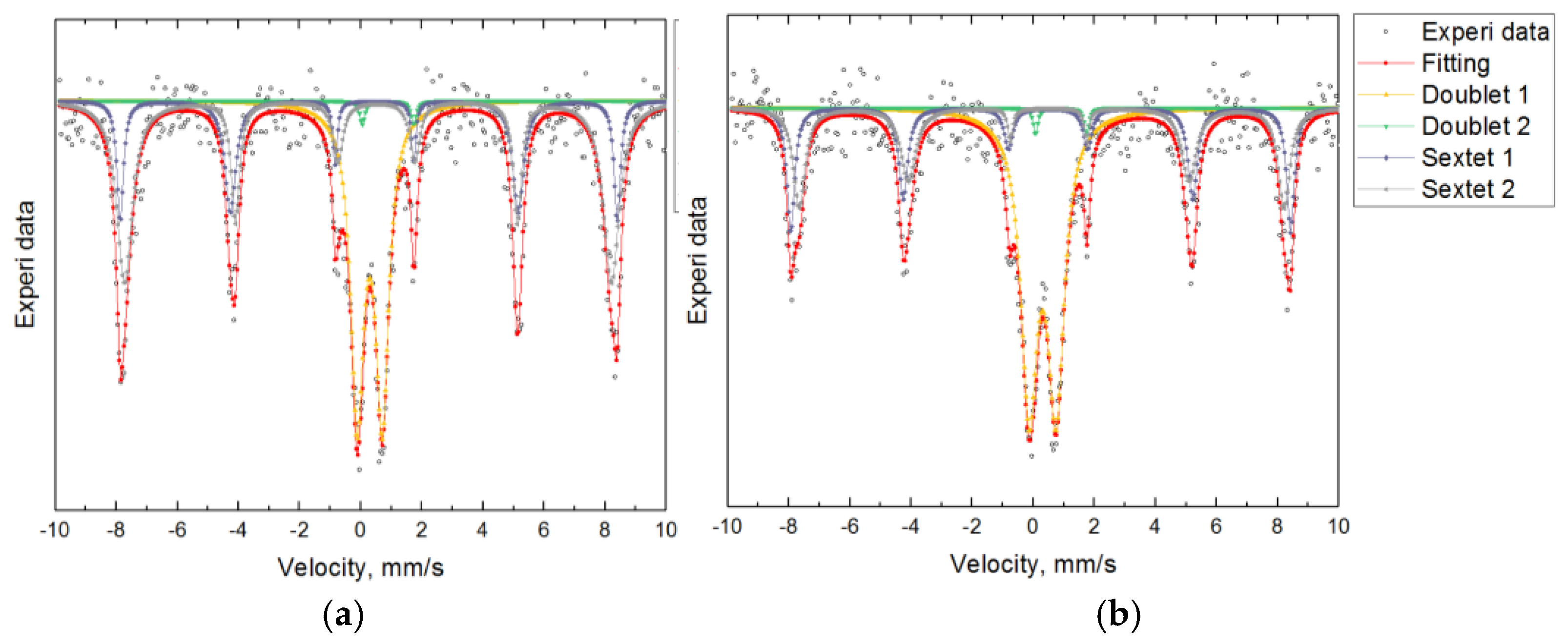
Figure 3.
Hysteresis loops and determination of coercivity from remanent magnetization of the samples Ind at 2 K (a) and 295 K (b), Lab at 2 K (c) and at 295 K (d), ClayL at 295 K (e). On insets: central parts of loops and remanent magnetization destruction curves.
Figure 3.
Hysteresis loops and determination of coercivity from remanent magnetization of the samples Ind at 2 K (a) and 295 K (b), Lab at 2 K (c) and at 295 K (d), ClayL at 295 K (e). On insets: central parts of loops and remanent magnetization destruction curves.
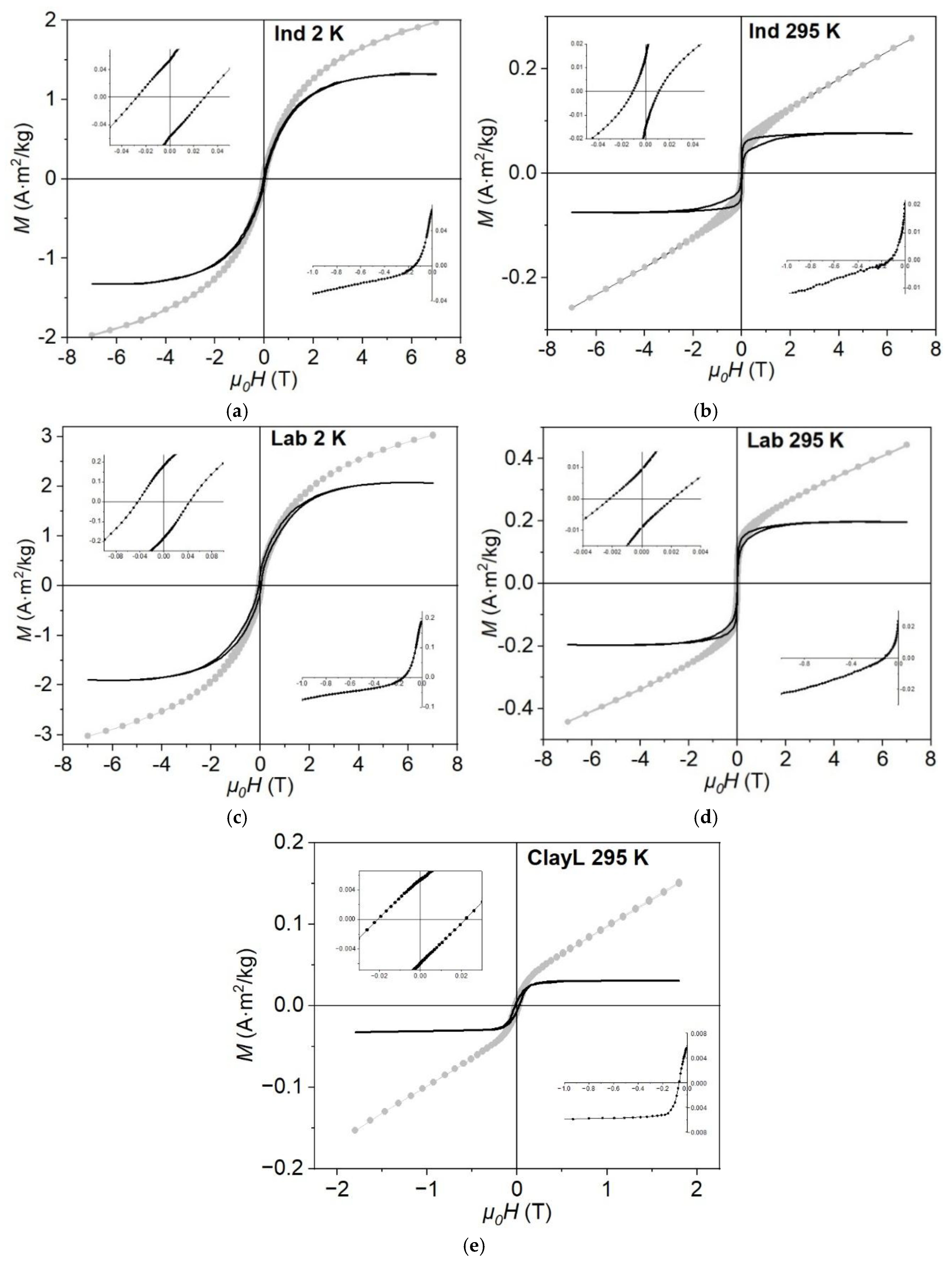
Figure 4.
ARM destruction (black) and its coercivity spectrum (gray) for samples Ind (a) and Lab (b).
Figure 4.
ARM destruction (black) and its coercivity spectrum (gray) for samples Ind (a) and Lab (b).
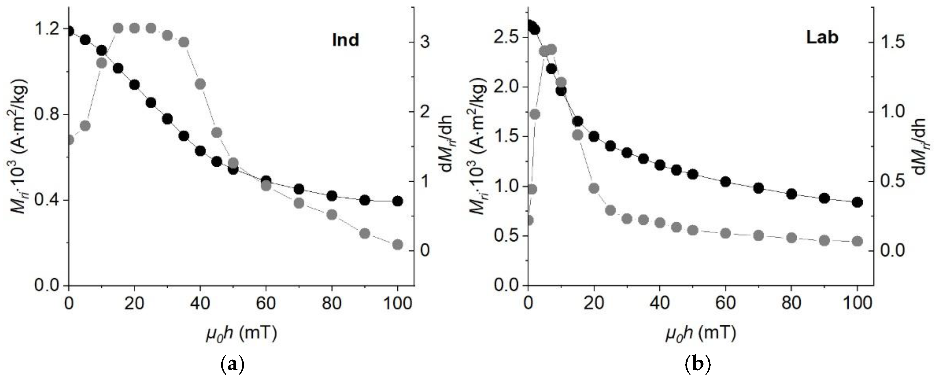
Figure 5.
Thermal demagnetization of 3-component IRM for Ind sample.
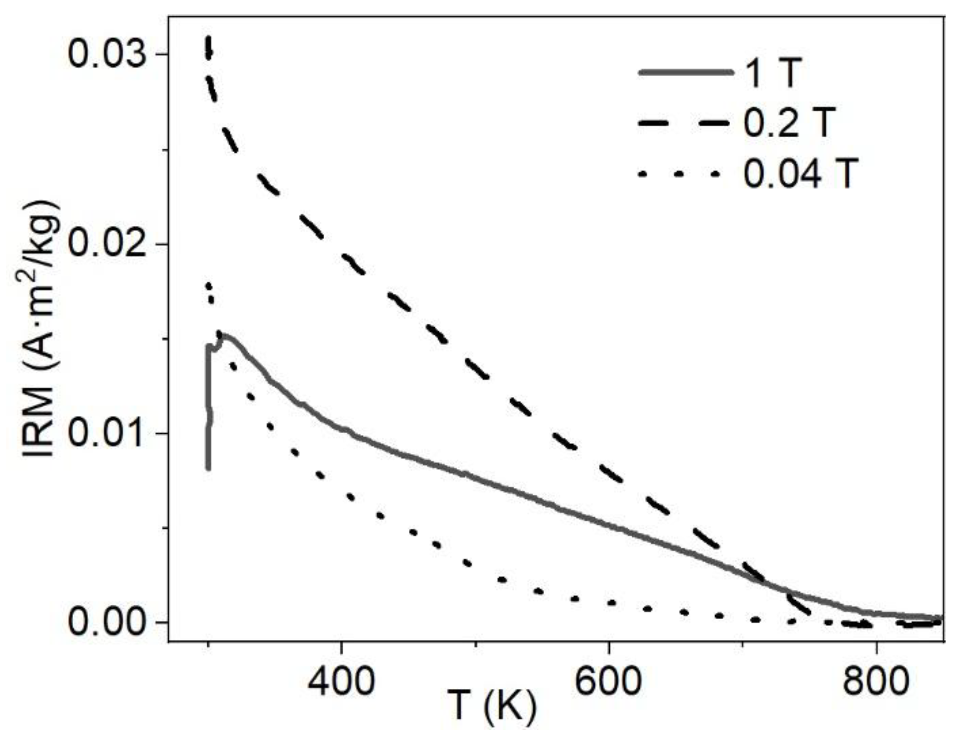
Figure 6.
Low-temperature magnetization measurements for Ind and Lab samples. LT-SIRM: gray FC, black ZFC; RT-SIRM blue curve.
Figure 6.
Low-temperature magnetization measurements for Ind and Lab samples. LT-SIRM: gray FC, black ZFC; RT-SIRM blue curve.
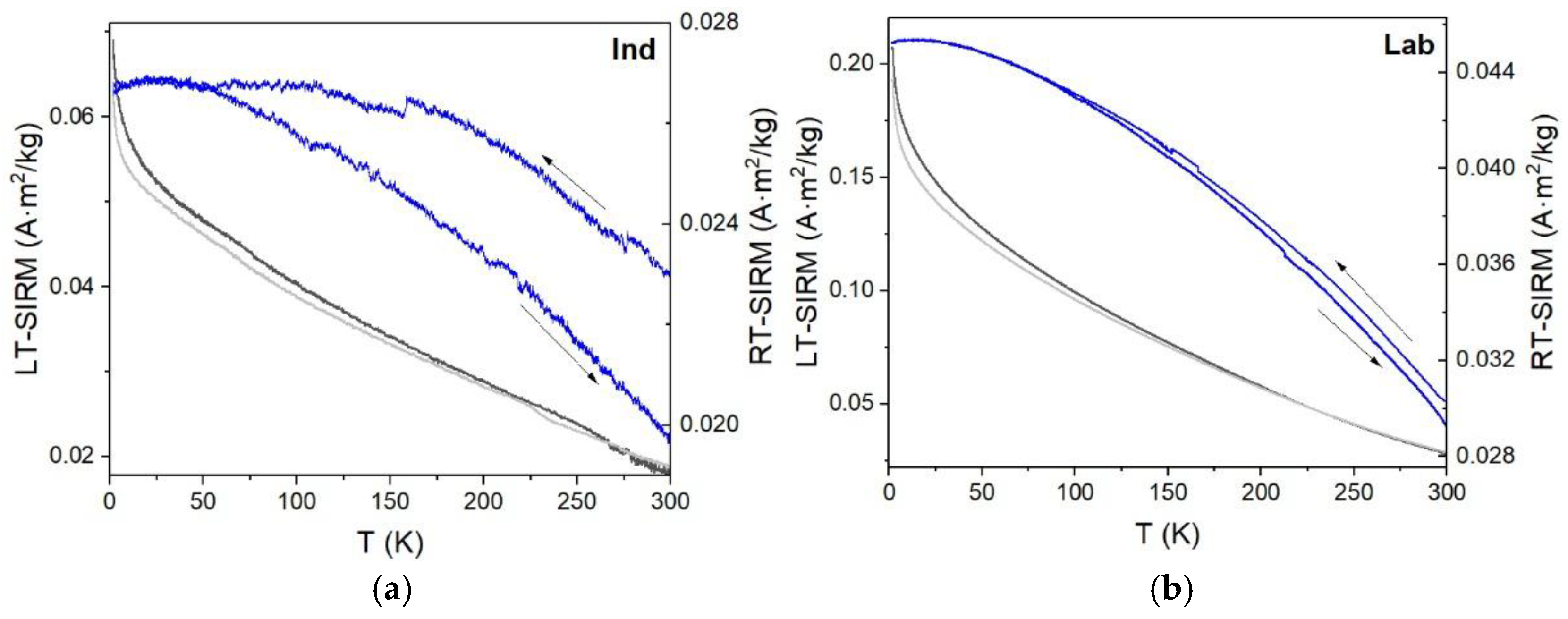
Figure 7.
Impulse transient characteristic of industrial brick sample (grey dots) and its power-law approximation in the time interval 25–1000 µs (blue line). The error estimate for the exponent b corresponds to standard deviation.
Figure 7.
Impulse transient characteristic of industrial brick sample (grey dots) and its power-law approximation in the time interval 25–1000 µs (blue line). The error estimate for the exponent b corresponds to standard deviation.
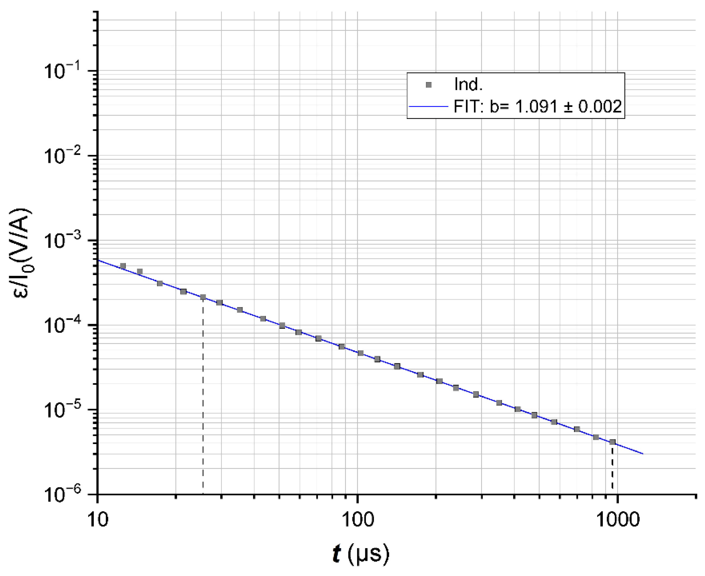
Figure 8.
Frequency-temperature dependencies of magnetic susceptibility of Ind (a) and Lab (b) samples.
Figure 8.
Frequency-temperature dependencies of magnetic susceptibility of Ind (a) and Lab (b) samples.
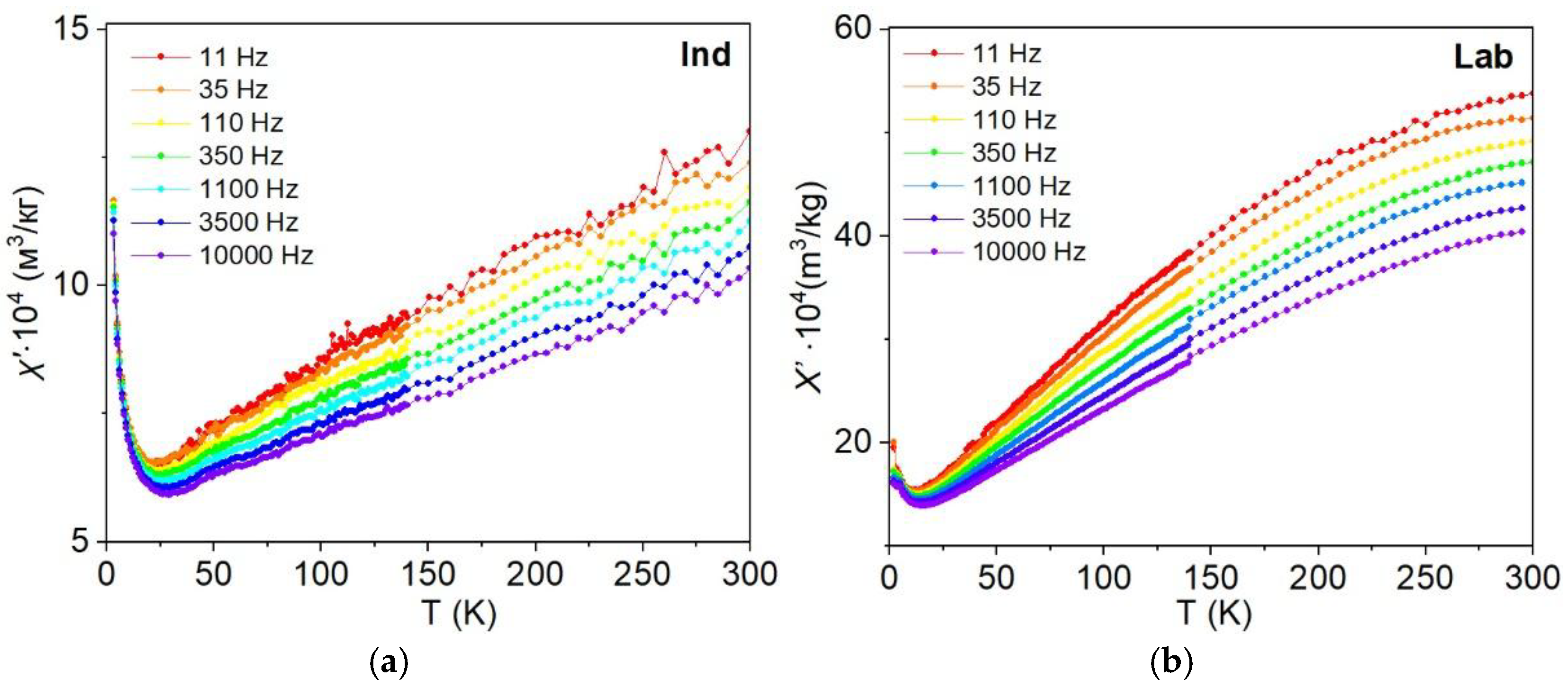
Figure 9.
Frequency-field dependencies of magnetic susceptibility of ClayL (a), Ind (b), and Lab (c) samples.
Figure 9.
Frequency-field dependencies of magnetic susceptibility of ClayL (a), Ind (b), and Lab (c) samples.
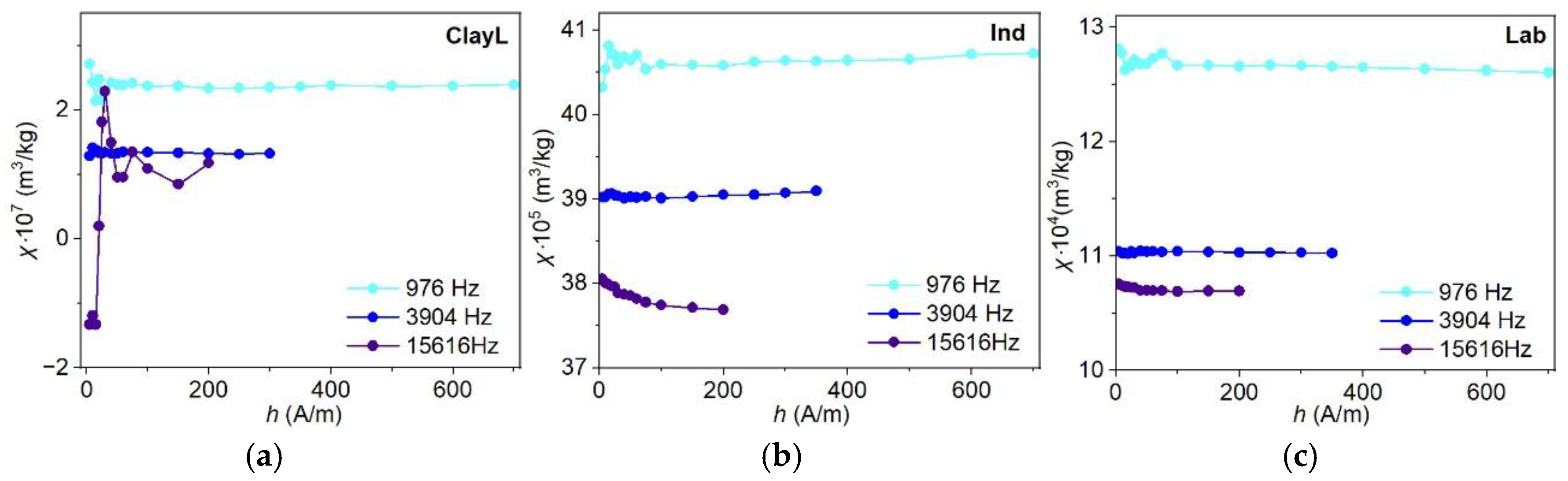
Table 1.
Quantitative phase analysis of the samples (wt. %) according to full profile analysis by Rietveld method.
Table 1.
Quantitative phase analysis of the samples (wt. %) according to full profile analysis by Rietveld method.
| ClayL | Ind | Lab | |
|---|---|---|---|
| Quartz | 40 | 44 | 49 |
| Feldspar (microcline + plagioclase) | 23 | 39 | 41 |
| Mica | 20 | 3 | 4 |
| Amphibole | 2 | 1 | 1 |
| Hematite | — | 5 | 5 |
| Spinel | — | 8 | — |
| Kaolinite | 9 | — | — |
| Pyroxene | 2 | — | — |
| Chlorite | 5 | — | — |
| Dolomite | 1 | — | — |
| Rp(*) (%) | 4.4 | 5.9 | 5.4 |
| (*) convergence factor of the calculated and experimental X-ray profiles, yi-intensity at each experimental point of the X-ray image. | |||
Table 2.
Parameters of Mössbauer spectra.
| Sample | Component | Fe | IS (mm/s) | QS (mm/s) | BHf (T) | % |
|---|---|---|---|---|---|---|
| Lab | Doublet Fe(1) | Fe3+ | 0.305±0.009 | 0.882±0.016 | — | 50.11 |
| Doublet Fe(2) | Fe2+ | 0.910±0.044 | 1.663±0.089 | — | 1.29 | |
| Sextet Fe(3) | Fe3+ | 0.363±0.012 | 0.241±0.023 | 50.796±0.097 | 22.82 | |
| Sextet Fe(4) | Fe3+ | 0.388±0.017 | 0.228±0.034 | 49.285±0.205 | 25.78 | |
| Ind | Doublet Fe(1) | Fe3+ | 0.293±0.007 | 0.819±0.012 | — | 36.92 |
| Doublet Fe(2) | Fe2+ | 0.895±0.057 | 1.675±0.115 | — | 1.13 | |
| Sextet Fe(3) | Fe3+ | 0.353±0.010 | 0.183±0.021 | 50.543±0.085 | 20.84 | |
| Sextet Fe(4) | Fe3+ | 0.372±0.010 | 0.274±0.021 | 49.496±0.132 | 41.11 |
Table 3.
Hysteresis characteristics of the samples. In parentheses in the Samples column, the measurement setup and the hysteresis measurement temperature in K are indicated.
Table 3.
Hysteresis characteristics of the samples. In parentheses in the Samples column, the measurement setup and the hysteresis measurement temperature in K are indicated.
| Sample | Ms, A⋅m2/kg | Mrs, A⋅m2/kg | Mrs/ Ms | μ0Hc, mT | μ0Hcr, mT | Hcr/ Hc |
|---|---|---|---|---|---|---|
| ClayL (Lake Shore 295) | 0.03 | 0.005 | 0.17 | 17 | 64 | 3.8 |
| Ind (MPMS 2) | 1.30 | 0.060 | 0.05 | 28 | 150 | 5.4 |
| Ind (MPMS 295) | 0.08 | 0.020 | 0.25 | 10 | 139 | 13.9 |
| Lab (MPMS 2) | 2.00 | 0.190 | 0.10 | 45 | 150 | 3.3 |
| Lab (MPMS 295) | 0.20 | 0.020 | 0.10 | 2 | 119 | 59.5 |
Table 4.
FD factor values at room temperature.
| Sample | fd, % | ||
|---|---|---|---|
| MFK1-FA | PPMS-9 | Average value | |
| Ind | 5.2 | 7.8 | 6.5 |
| Lab | 12.5 | 8.5 | 10.5 |
| ClayL | 50 (estimation) | – | – |
Disclaimer/Publisher’s Note: The statements, opinions and data contained in all publications are solely those of the individual author(s) and contributor(s) and not of MDPI and/or the editor(s). MDPI and/or the editor(s) disclaim responsibility for any injury to people or property resulting from any ideas, methods, instructions or products referred to in the content. |
© 2025 by the authors. Licensee MDPI, Basel, Switzerland. This article is an open access article distributed under the terms and conditions of the Creative Commons Attribution (CC BY) license (http://creativecommons.org/licenses/by/4.0/).
Copyright: This open access article is published under a Creative Commons CC BY 4.0 license, which permit the free download, distribution, and reuse, provided that the author and preprint are cited in any reuse.


