
Submitted:
10 October 2025
Posted:
14 October 2025
You are already at the latest version
Abstract
This article presents a deterministic model describing the joint dynamics of canine and human rabies in a cross-border context. This model explicitly integrates dog mobility between two neighboring countries and allows for the evaluation of the impact of these movements on disease persistence. We analyze the basic reproduction number \(\mathcal{R}_0\), study the local and global stability of equilibrium points, identify the most influential parameters through sensitivity analysis, and perform numerical simulations to test the effectiveness of various vaccination and movement control strategies.
Keywords:
rabies
; mathematical modeling
; basic reproduction number
; sensitivity analysis
; numerical simulation
1. Introduction
Rabies is a fatal viral zoonosis primarily affecting mammals, including humans. It is responsible for nearly 59,000 human deaths per year worldwide, the majority occurring in Africa and Asia, with dogs being responsible for over 99% of human transmissions [1,2]. Prevention mainly relies on vaccination of reservoir animals, particularly dogs, and post-exposure prophylaxis in humans. Numerous studies have confirmed that mass dog vaccination is the most effective tool for interrupting transmission, often more cost-effective than solely strengthening post-exposure prophylaxis [3,4].
However, cross-border mobility of dogs complicates control strategies, especially in border regions where inter-state coordination is often weak. For example, studies conducted at the border between Chad and Cameroon have shown the importance of considering canine migratory flows to understand the spatial dynamics of rabies [5,6]. In the Serengeti region, analyses have highlighted that regular reintroductions of the disease from neighboring areas can compromise local efforts, making large-scale vaccination necessary [7].
In several regions of the world, notably in Africa and Asia, vaccination efforts are fragmented. Models applied to African urban contexts [8] or to China [9,10] have shown that vaccination coverage must exceed a critical threshold (often ≥ 70 %) to guarantee elimination, and that high turnover in the dog population leads to a rapid decline in coverage if campaigns are not repeated annually [11].
Mathematical models have improved the understanding of rabies transmission, particularly compartmental models of the SIR [12] or SEIR type adapted to animal and human contexts [13]. These works also highlight the importance of integrating the dynamics of canine and human populations within a realistic spatial framework. However, few studies have explored the impact of cross-border dog exchanges in a multi-country setting, even though this approach is crucial for achieving the goals of the WHO’s "Zero human deaths from dog-mediated rabies by 2030" strategy [1].
The aim of this study is to propose a multi-country mathematical model for canine rabies, accounting for dog movements between two neighboring countries to better understand the impact of cross-border mobility on disease dynamics and to evaluate the effectiveness of different control strategies.
Our specific objectives include, among others:
Developing a compartmental model structured by country, integrating bidirectional dog movements between the two countries;
Calculating and analyzing the basic reproduction number for this multi-country system;
Studying the stability of the rabies-free equilibrium and the conditions for endemic persistence in each country;
Performing a sensitivity analysis to identify the most influential parameters on rabies spread;
Simulating the effect of different targeted vaccination and movement control strategies.
2. Model Formulation
To describe the dynamics of rabies in two interconnected countries, we construct a compartmental model structured into two subpopulations (human and canine) for each country denoted (home country) and (neighboring country) [14]. The model is inspired by previous work on canine rabies dynamics and cross-species transmission between dogs and humans [15,16,17].
For each country i,
- The canine population is divided into compartments: susceptible (), exposed (), infectious (), vaccinated ().
- The human population is divided into susceptible (), exposed (), and infected ().
- Vaccination is applied only to dogs.
- The model is formulated for two interconnected countries .
- Dog movements between countries are negligible.
2.1. Flow Diagram
Figure 1.
illustrates the flow diagram of the model, showing transitions between compartments for canine and human populations in both countries. Arrows indicate transmission pathways, infection progression, vaccination, as well as demographic movements.
Figure 1.
illustrates the flow diagram of the model, showing transitions between compartments for canine and human populations in both countries. Arrows indicate transmission pathways, infection progression, vaccination, as well as demographic movements.
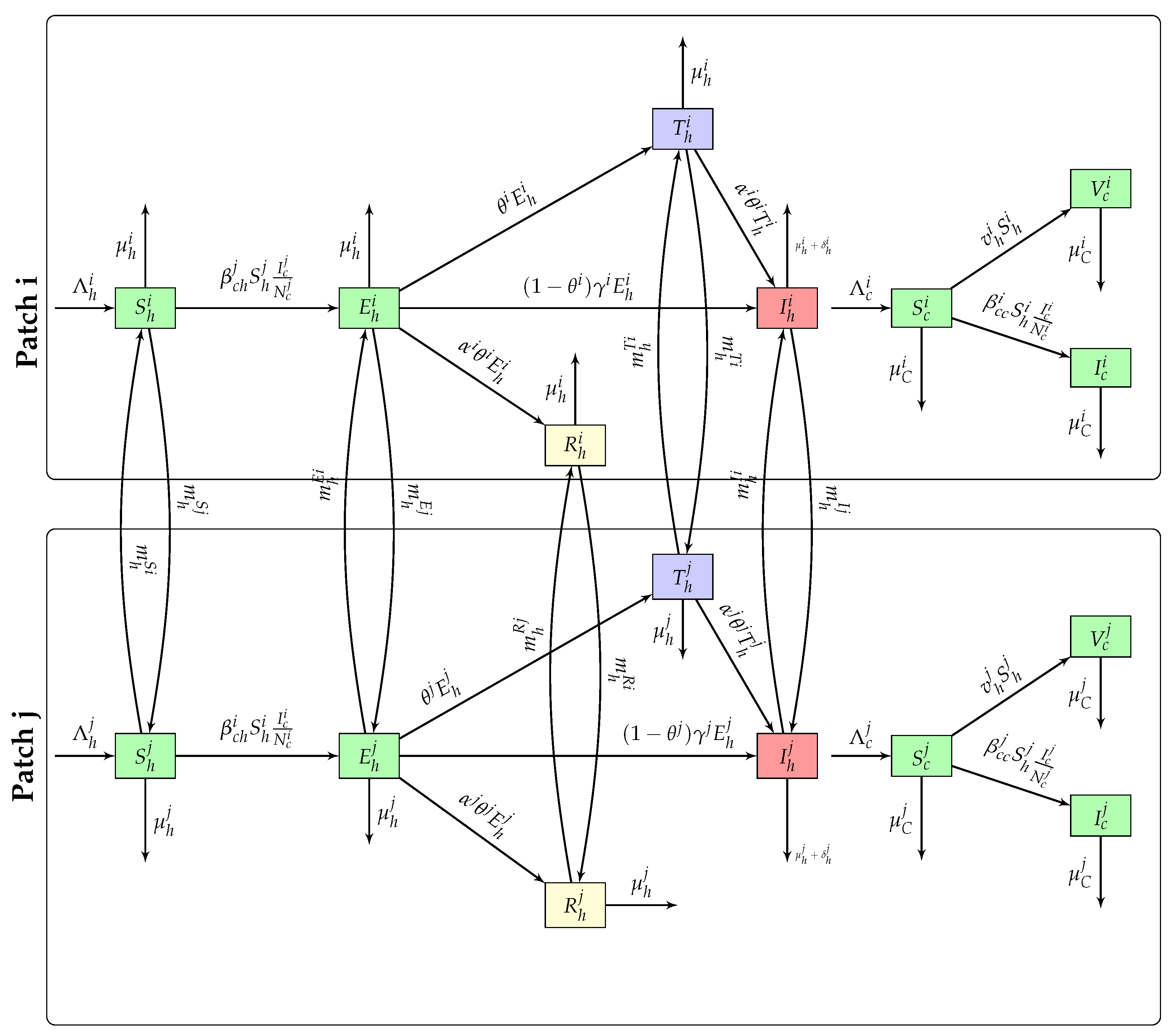

Table 1.
Model variables for each country .
| Variable | Description |
|---|---|
| Number of susceptible dogs in country i | |
| Number of exposed dogs in country i | |
| Number of infected dogs in country i | |
| Number of vaccinated dogs in country i | |
| Number of susceptible humans in country i | |
| Number of exposed humans in country i | |
| Number of treated humans in country i | |
| Number of infected humans in country i | |
| Number of recovered humans in country i |
Table 2.
Model parameters.
| Parameter | Description |
|---|---|
| Human recruitment rate in country i | |
| Dog recruitment rate in country i | |
| Dog-to-human transmission rate | |
| Dog-to-dog transmission rate | |
| Natural mortality rate of dogs | |
| Vaccine efficacy | |
| Canine vaccination rate | |
| Disease-induced mortality rate in dogs | |
| Probability of receiving post-exposure treatment | |
| Natural mortality rate of humans | |
| Progression rate to infection in humans | |
| Disease-induced mortality rate in humans | |
| Migration rates (humans, dogs) between countries |
The systems of equations are given by:
Dogs
Humans
3. Model Analysis
3.1. Vector Form
Before proceeding further, let us specify some vector and matrix notations that will be used subsequently.
Vectors are assumed to be column vectors but are written without specific orientation unless otherwise indicated [14]. If , then means that , means that and there exists at least one i such that ; finally, means that for all . For , we have , and if, respectively, , and . This same notation applies to matrices.
Writing system (Section 2) in vector form is particularly useful for the remainder of the work. We therefore introduce some notations here.
For any variable , we denote , and we define:
as the vector of state variables.
We also introduce the following notations:
Finally, for each compartment , the associated movement matrix is given by:
Movement matrices of the form (2) possess many useful properties for the analysis of metapopulation systems [14,18], which we will use later in the analysis.
We denote ∘ as the Hadamard product (element-wise product).
3.2. Positivity
Theorem 3.1.
The components are positive for all time t.
Proof.
Equation (1e) implies . Its vector form gives , where denotes the movement matrix of susceptible canines. The solution to this differential equation is
with .
Similarly, the solution to Equation (1a) is given by
with . □
Theorem 3.2.
The total human and canine populations are bounded for all positive time t.
Proof.
Define the total human population of country i: .
Summing equations (1e)-(1i), we obtain:
This differential inequality is linear, and its solution is
Thus:
− If , then .
− If , then .
Therefore:
The same reasoning applies to the total canine population:
Thus, all human and canine populations are not only positive but also uniformly bounded in time. □
3.3. Isolated Case
This section considers the initial model without movement.
3.3.1. Disease-Free Equilibrium
The analysis of equilibrium points of a dynamical system allows for the identification of stationary states in which populations no longer vary over time.
Then, by setting the differential equations to zero and assuming the absence of infected or exposed individuals , we obtain:
Thus, we have two disease-free equilibrium points:
3.3.2. Basic Reproduction Number in an Isolated Location
To calculate the basic reproduction number,
We use the Next Generation Matrix method by van den Driessche and Watmough [19].
We consider the following infectious variables for country i, .
The dynamics of these variables are decomposed into two functions:
- : rate of appearance of new infections in each compartment and
- : rate of transition between compartments (exits and entries due to progression or recovery),
which are given by:
We compute the Jacobian of F and V at the disease-free equilibrium (DFE), i.e., when .
The Jacobian of and at the DFE are:
We define the next generation matrix :
The basic reproduction number is the spectral radius (dominant eigenvalue) of . Here, we have:
Remark 3.1.
This model assumes that humans do not retransmit rabies, which is biologically correct (rabies is not transmissible between humans). This is why is not a source of new infections, and humans do not fuel the epidemic reproduction dynamics.
3.3.3. Local Stability Analysis
Theorem 3.3.
The disease-free equilibrium point is locally asymptotically stable when and unstable otherwise.
Proof.
The Jacobian matrix evaluated around the DFE is given by
The stability of the DFE depends on the sign of the eigenvalues of this matrix. We can see:
The 2×2 submatrix in the top left is triangular, so its eigenvalues are:
The last eigenvalue (related to ) is:
Then, if , . So all eigenvalues have negative real parts. Therefore, the disease-free equilibrium is locally asymptotically stable.
But, if , . And since one of the eigenvalues is positive, then the disease-free equilibrium is unstable. □
3.3.4. Global Stability of the Disease-Free Equilibrium
Theorem 3.4.
The disease-free equilibrium is globally asymptotically stable if .
Proof.
Let us verify the conditions of the Castillo-Chavez theorem.
-
Let be the class of uninfected individuals, and the class of infected individuals.For , the system becomes:Solving these equations:i.e.,andTaking the limit as , we obtain:So is globally stable when .
-
Now consider the system for infected individuals:Let , we have:Thenbecause from (13) and (9)
Thus, is globally asymptotically stable when . □
3.4. Analytical Calculation of the Critical Vaccination Threshold
If
the condition implies:
We define:
- If , then : no vaccination effort required to ensure (theoretical viewpoint).
- If , then gives the minimal vaccination rate to achieve in steady state to obtain .
Practical remark: this threshold is a theoretical guide; in reality, one must account for actual coverage, vaccine efficacies, parameter uncertainties, and logistics.
Corollary 3.1.(Critical canine vaccination threshold) From the expression
the condition provides a minimal threshold for the vaccination rate , denoted , such that if then .
Explicit formula:
Proof.
Condition on for . We start from
- -
-
Isolate : Multiply by :Divide by :Isolate :
- -
- Negative case: if , the right-hand side is , so a rate satisfies . Otherwise, a positive minimal vaccination effort is required.
- -
- Compact formulation:
□
3.4.1. Equivalent Expression for Vaccination Coverage p
We express p as the proportion of vaccinated dogs at equilibrium:
Solving for :
Substitute into :
The condition becomes:
Critical coverage:
We verify that this corresponds to :
3.4.2. Generalization: Imperfect Vaccine
If the vaccine has an efficacy , the protected fraction is and the remaining fraction is .
The condition becomes:
3.5. Disease-Free Equilibrium
Then, by setting the differential equations of system Section 3.1 to zero and assuming the absence of infected or exposed individuals , and noting that the matrix is non-singular and thus invertible, we obtain:
Thus, we have two disease-free equilibrium points:
3.6. Basic Reproduction Number for the Global System
3.7. Local Stability
First, from [19], we have the following result.
Theorem 3.5.
is locally asymptotically stable if and unstable if .
Proof.
We need to verify that assumptions A1-A5 of [19] are satisfied. Assumptions A1-A4 follow from the procedure used above to derive F and V in the calculation of . Therefore, all we need to verify is that the disease-free system at the DFE is locally asymptotically stable. In the absence of disease, (Section 3.1) is a linear system
This is exactly (Section 3.5), so we know it has a unique equilibrium, the disease-free equilibrium (19). The Jacobian matrix of the system at any point takes the form
We saw in Section 3.1 that this matrix is invertible. According to [18], the spectral abscissa of this matrix is negative, so the disease-free equilibrium is always (locally) asymptotically stable. The result then follows. □
4. Sensitivity Analysis
We use the data from Table 3 for our numerical simulations.
Figure 2.
PRCC of .
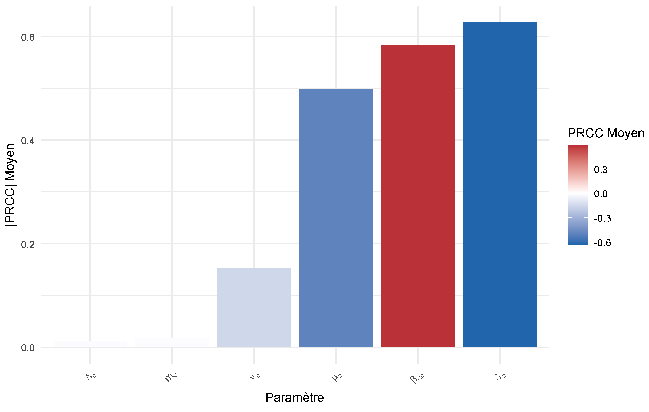
Interpretation: This analysis reveals which parameters to target for effective interventions:
Parameters with high positive PRCC represent priority targets for reduction measures (e.g., decreasing transmission rates). Parameters with high negative PRCC represent intervention opportunities (e.g., increasing vaccination or treatment rates).
5. Numerical Simulations
To visualize the temporal dynamics of the model and understand the impact of the basic reproduction number (), we performed numerical simulations for canine and human populations. Two contrasting scenarios were studied: one where , indicating the epidemic is theoretically controlled, and another where , a scenario in which the disease can spread within the population.
6. Discussion
Figure 3 shows the dynamics for . A rapid epidemic is observed: the infected compartment () experiences rapid exponential growth, peaking at a high level where a large portion of the population is simultaneously infected. Subsequently, the number of infected decreases as the pool of susceptibles () is depleted, either by infection or vaccination. This curve is characteristic of an uncontrolled epidemic.
Conversely, Figure 4 illustrates the scenario where . Here, the number of infected decreases monotonically from the start, without an epidemic peak. Each infected individual generates on average less than one new infection, leading to the natural and rapid extinction of the disease. The vaccinated population () remains significant, contributing to herd immunity. This result validates the theoretical threshold: if , the disease cannot be maintained in the population.
The impact of the two canine scenarios on public health is striking. Figure 5 shows that an uncontrolled canine epidemic () leads to a significant risk for humans (), resulting in an increase in cases of exposure (), infection (), and requiring treatment ().
In contrast, Figure 6 demonstrates the beneficial effect of controlling rabies at its animal source. When , transmission from dog to human is interrupted, as evidenced by the value . The curves for the exposed, infected, and treated compartments remain consistently at negligible, or even zero, levels. The human population remains mostly, if not entirely, in the susceptible () or immune () compartment, confirming that the best strategy to protect humans is to massively vaccinate dogs.
These results highlight the critical relationship between disease control in the animal reservoir (the dog) and the risk to human health. They emphasize the importance of maintaining sufficient canine vaccination coverage to ensure that remains sustainably below 1, in order to prevent both canine epidemics and human rabies cases.
7. Conclusion
This study developed and analyzed a metapopulation-type mathematical model for the dynamics of canine and human rabies in a cross-border context. The theoretical analysis allowed for the determination of the basic reproduction number, , whose threshold value of 1 governs the stability of the disease-free equilibrium. The results rigorously demonstrate that this equilibrium is locally and globally asymptotically stable when , guaranteeing epidemic extinction, and unstable otherwise, leading to endemic persistence. Sensitivity analysis identified the parameters most influential on , such as the inter-canine transmission rate () and the vaccination rate (), thus providing priority targets for intervention strategies.
Numerical simulations concretely illustrated the crucial impact of canine vaccination. An insufficient vaccination rate, leading to , results in an explosive epidemic in the canine population, which immediately translates into an increased risk of transmission to humans. Conversely, vaccination coverage exceeding the critical threshold, ensuring , effectively extinguishes transmission in both dogs and humans. These results underscore the imperative necessity of cross-border coordination and massive, sustained dog vaccination campaigns as a central strategy to achieve the global goal of "Zero human deaths from dog-mediated rabies by 2030".
References
- Organization, W.H. Zero by 30: The global strategic plan to end human deaths from dog-mediated rabies by 2030, 2018.
- Hampson, K.; Coudeville, L.; Lembo, T.; et al. Estimating the global burden of endemic canine rabies. PLoS Neglected Trop. Dis. 2015, 9, e0003709. [Google Scholar]
- Zinsstag, J.; Durr, S.; Penny, M.A.; Mindekem, R.; Roth, F.; Gonzalez, S.M.; Naissengar, S.; Hattendorf, J. Transmission dynamics and economics of rabies control in dogs and humans in an African city. Proc. Natl. Acad. Sci. 2009, 106, 14996–15001. [Google Scholar] [CrossRef] [PubMed]
- Beyer, H.L.; Hampson, K.; Lembo, T.; et al. . Cost-effectiveness of dog rabies vaccination programs in East Africa. PLoS Neglected Trop. Dis. 2018, 12, e0006490. [Google Scholar] [CrossRef]
- Lechenne, M.; Mindekem, R.; et al. The importance of a participatory and integrated one health approach for rabies control: The case of N’Djamena, Chad. Trop. Med. Infect. Dis. 2017, 2, 43. [Google Scholar] [CrossRef] [PubMed]
- Zinsstag, J.; Lechenne, M.; et al. Transmission dynamics and economics of rabies control in dogs and humans in an African city. Proc. Natl. Acad. Sci. 2017, 114, 13510–13515. [Google Scholar] [CrossRef] [PubMed]
- Lushasi, K.; Hampson, K.; Cleaveland, S.; et al. Rabies shows how scale of transmission can enable acute zoonoses to persist in endemic settings. Proc. Natl. Acad. Sci. 2020, 117. [Google Scholar]
- Hampson, K.; et al. . Vaccination of dogs in an African city interrupts rabies transmission and reduces human exposure. Sci. Transl. Med. 2017, 9, eaaf6984. [Google Scholar] [CrossRef]
- Zhang, J.; Jin, Z.; Sun, G.Q.; Zhou, T.; Ruan, S. Modeling the transmission dynamics and control of rabies in China. Math. Biosci. 2017, 286, 65–93. [Google Scholar] [CrossRef] [PubMed]
- Nguyen, Q.; Li, X.; Wang, Y.; et al. Dynamic analysis of rabies transmission and elimination in dogs and humans in China. Infect. Dis. Model. 2023, 8. [Google Scholar]
- Samanta, S.; Mushayabasa, S.; Ghosh, D.; et al. System dynamics modelling approach to explore the effect of dog demography on rabies vaccination coverage decline. PLoS ONE 2018, 13, e0205884. [Google Scholar] [CrossRef]
- Abdramane, A.; Djimramadji, H.; Daoussa Haggar, M. Study of the Dynamics of HIV-Cholera Co-Infection in a Mathematical Model. Electron. J. Math. Anal. Appl. 2025, 13, 1–11. [Google Scholar] [CrossRef]
- Bourhy, H.; Dacheux, L.; et al. The origin and phylogeography of dog rabies virus. J. Gen. Virol. 2016, 97, 2691–2703. [Google Scholar] [CrossRef] [PubMed]
- Saad, A.A.; Arino, J.; Tchepmo Djomegni, P.M.; Daoussa Haggar, M.S. A metapopulation model for the spread of cholera. arXiv 2025, arXiv:2505.17269. [Google Scholar] [CrossRef]
- Hossain, M.J.; Ahmed, T.; Bulbul, T.; Rahman, M.; Hampson, K.; Alonso, W.J.; Rupprecht, C.E. Modelling the effectiveness of dog rabies vaccination programmes in Asian countries: A case study from Bangladesh. Infect. Dis. Poverty 2020, 9, 1–10. [Google Scholar]
- Lembo, T.; Hampson, K.; Kaare, M.T.; Ernest, E.; Knobel, D.; Kazwala, R.R.; Coleman, P.G.; Cleaveland, S. Modeling the impact of dog vaccination on human rabies transmission in Africa. PLoS Neglected Trop. Dis. 2010, 4, e725. [Google Scholar]
- Zinsstag, J.; Dürr, S.; Penny, M.A.; Mindekem, R.; Roth, F.; Menendez Gonzalez, S.; Naissengar, S.; Hattendorf, J. Transmission dynamics and economics of rabies control in dogs and humans in an African city. Proc. Natl. Acad. Sci. 2009, 106, 14996–15001. [Google Scholar] [CrossRef] [PubMed]
- Arino, J.; Bajeux, N.; Kirkland, S. Number of Source Patches Required for Population Persistence in a Source–Sink Metapopulation with Explicit Movement. Bull. Math. Biol. 2019, 81, 1916–1942. [Google Scholar] [CrossRef] [PubMed]
- van den Driessche, P.; Watmough, J. Reproduction numbers and sub-threshold endemic equilibria for compartmental models of disease transmission. Math. Biosci. 2002, 180, 29–48. [Google Scholar] [CrossRef] [PubMed]
Figure 3.
Dynamics of infection in the canine population for . A major epidemic is observed with a significant peak of infected individuals ().
Figure 3.
Dynamics of infection in the canine population for . A major epidemic is observed with a significant peak of infected individuals ().
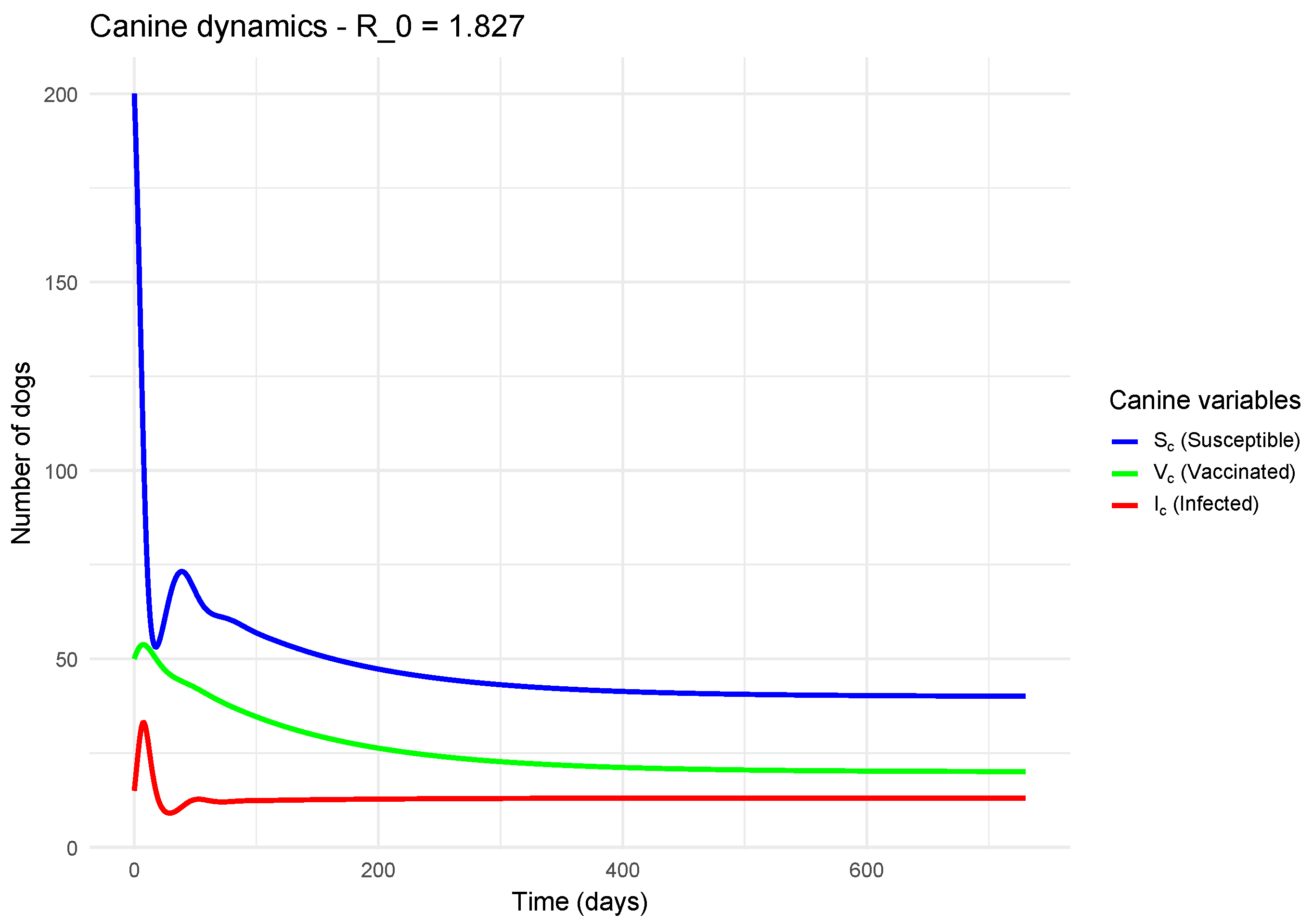
Figure 4.
Dynamics of infection in the canine population for . The epidemic does not take off; the number of infected () rapidly decreases towards zero.
Figure 4.
Dynamics of infection in the canine population for . The epidemic does not take off; the number of infected () rapidly decreases towards zero.
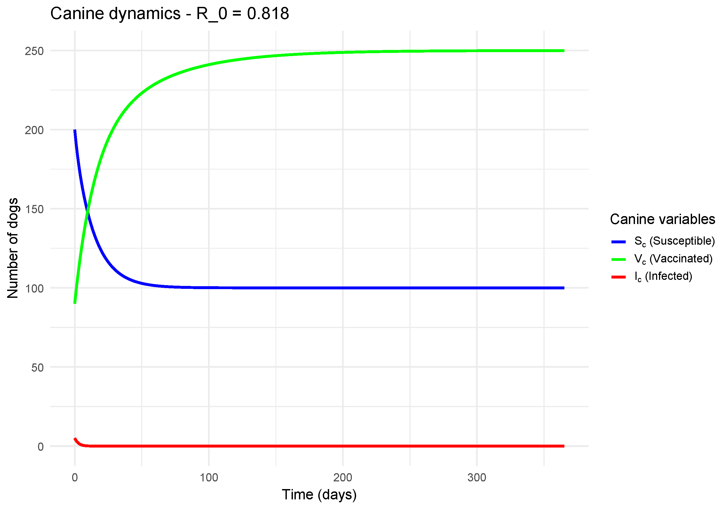
Figure 5.
Dynamics of infection in the human population resulting from an uncontrolled canine epidemic ().
Figure 5.
Dynamics of infection in the human population resulting from an uncontrolled canine epidemic ().
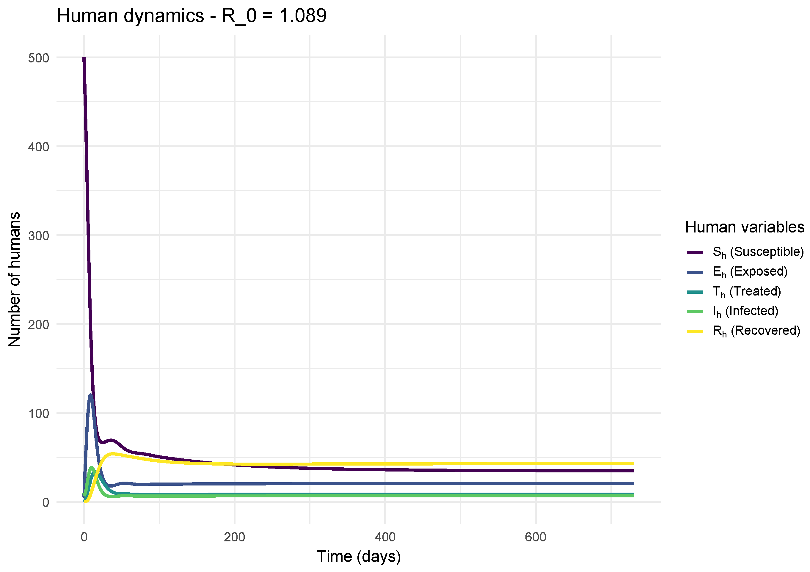
Figure 6.
Dynamics of infection in the human population resulting from a controlled canine epidemic (). The risk of transmission to humans is extremely low.
Figure 6.
Dynamics of infection in the human population resulting from a controlled canine epidemic (). The risk of transmission to humans is extremely low.
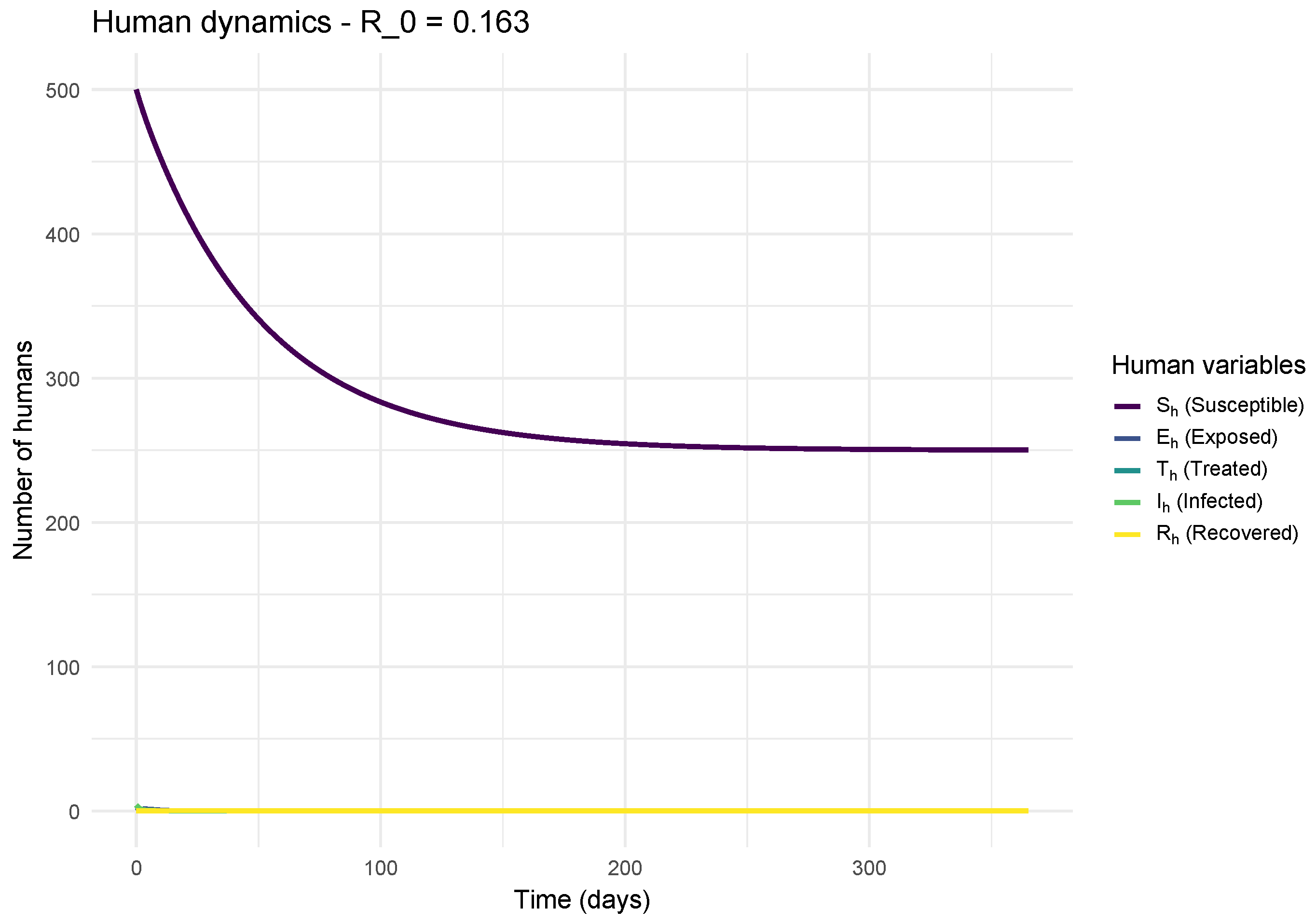
Table 3.
Revised model parameters.
| Parameters | Intervals | Values | References |
|---|---|---|---|
| - | 0.027 | Local data | |
| - | 0.5-1 | Estimation | |
| 0.000004-0.15 | 0.0001 | Adapted to data | |
| 0.1-0.5 | 0.3 | Realistic estimation | |
| 0.1-0.3 | 0.2 | Demographic data | |
| 0.05-0.2 | 0.1 | Estimation | |
| 0.01-0.1 | 0.05 | Vaccination program | |
| 0.5-1 | 0.8 | Canine rabies data | |
| 0.001-0.01 | 0.005 | Estimation | |
| 0.00003-0.00005 | 0.00004 | Demographic data | |
| 0.1-0.33 | 0.2 | Rabies incubation data | |
| 0.9-1 | 0.99 | Rabies mortality 100% | |
| 0.001-0.01 | 0.005 | Migration estimation |
Disclaimer/Publisher’s Note: The statements, opinions and data contained in all publications are solely those of the individual author(s) and contributor(s) and not of MDPI and/or the editor(s). MDPI and/or the editor(s) disclaim responsibility for any injury to people or property resulting from any ideas, methods, instructions or products referred to in the content. |
© 2025 by the authors. Licensee MDPI, Basel, Switzerland. This article is an open access article distributed under the terms and conditions of the Creative Commons Attribution (CC BY) license (http://creativecommons.org/licenses/by/4.0/).
Copyright: This open access article is published under a Creative Commons CC BY 4.0 license, which permit the free download, distribution, and reuse, provided that the author and preprint are cited in any reuse.


