
Submitted:
13 October 2025
Posted:
14 October 2025
You are already at the latest version
Abstract
The Baltic Dry Index (BDI) measures the cost of transporting dry bulk commodities such as coal, iron ore, and grain. As a key indicator of global trade, supply chain dynamics, and overall economic activity, accurate short-term forecasting of the BDI is crucial.
This paper compares four univariate methods to obtain a more precise short-term BDI prediction model, providing valuable insights for decision-makers. Four forecasting tech-niques include Grey Forecast, ARIMA, Support Vector Regression (SVR), and EMD-SVR-GWO. Model performance is evaluated using three common metrics: Mean Absolute Error (MAE), Root Mean Squared Error (RMSE), and Mean Absolute Percentage Error (MAPE).
Our findings reveal that the novel EMD-SVR-GWO model outperforms the other univari-ate methods, demonstrating superior accuracy in forecasting monthly BDI trends. This study contributes to improved BDI prediction, aiding managers in strategic planning and decision-making.
Keywords:
univariate forecasting models
; Baltic dry index
; empirical mode decomposition
; support vector regression
; grey wolf optimizer
1. Introduction
The Baltic Dry Index (BDI) serves as a critical barometer for the global shipping industry, reflecting the costs of transporting dry bulk commodities such as coal, iron ore, and grain. As an economic indicator, the BDI provides valuable insights into the health of global trade, supply chain dynamics, and overall economic activity. Given its relevance, accurate forecasting of the BDI is of paramount importance for a diverse range of stakeholders, including shipping companies, commodity traders, investors, policymakers, and economists.
Historically, the BDI has exhibited significant volatility, influenced by a myriad of factors. These factors include global economic cycles, seasonal demand fluctuations, geopolitical events, and changes in shipping capacity. For instance, economic downturns often lead to reduced demand for raw materials, subsequently lowering shipping rates and the BDI. Conversely, periods of economic growth drive up demand for commodities, resulting in higher shipping rates. Additionally, events such as trade disputes, natural disasters, and changes in regulatory environments can cause sudden and unpredictable movements in the BDI. This volatility poses substantial challenges for forecasting but also presents opportunities for leveraging advanced analytical techniques to improve prediction accuracy.
Traditional forecasting methods, such as time series analysis and econometric models, have been employed with varying degrees of success in predicting BDI movements. These methods provide a foundation for understanding past trends and making short-term forecasts, they often struggle to capture the complex, non-linear relationships inherent in the factors influencing the BDI.
In recent years, advancements in machine learning and artificial intelligence have opened new avenues for improving forecast accuracy. Techniques such as artificial neural networks (ANNs), support vector machines (SVMs), and ensemble learning methods offer the potential to model complex patterns and interactions that traditional methods may overlook. These contemporary approaches can incorporate a wider range of variables and are capable of learning from large datasets, making them well-suited for forecasting highly volatile indices like the BDI.
Forecasting the Baltic Dry Index (BDI) is crucial for the shipping industry as it offers insights into global trade trends, aiding in fleet management, capacity planning, and route optimization. Accurate BDI forecasts help shipping companies reduce costs, improve efficiency, and make informed investment decisions. Additionally, understanding shipping demand trends aids in predicting commodity prices and managing risks, ultimately enhancing the competitiveness and operational efficiency of shipping companies. Thus, forecasting BDI has attracted considerable attention from both academic researchers and industry practitioners. The primary objective of this study is to compare various univariate forecasting techniques in order to develop a more accurate short-term prediction model for the BDI, offering practical insights for the shipping sector.
2. Literature Review
BDI forecasting methods can be broadly categorized into three groups: conventional econometric models, nonlinear models and machine learning techniques, and ensemble machine learning methods. These approaches have become the most widely adopted methodologies for BDI analysis in academic research.
2.1. Econometric Model
Econometric models were among the first developed for BDI forecasting, and they have been widely employed in validation studies. Both univariate and multivariate econometric methodologies are commonly applied in this research. Previous studies frequently utilized models such as the vector error correction model (VECM), vector autoregressive (VAR), and autoregressive integrated moving average (ARIMA). For instance, Veenstra and Franses [1] developed a time series-based VAR model to forecast the BDI, identifying non-stationarity in the data, which raised concerns about the stability of various modeling techniques. Cullinane et al. [2] used the ARIMA model for modifications to the Baltic Freight Index (BFI), demonstrating its superior predictive power. Kavussanos and Alizadeh [3] examined the seasonality of dry bulk freight rates, employing seasonal ARIMA and VAR models to assess fluctuations across different vessel sizes. Tsioumas et al. [4] introduced a multivariate vector autoregressive model with exogenous variables (VARX), which outperformed ARIMA in improving BDI forecasting accuracy. Zhang et al. [5] compared ARIMA, ARIMA-GARCH models, and artificial neural networks (ANNs), noting that econometric models performed better in one-step-ahead forecasts, while ANN-based algorithms achieved a higher direction matching rate in weekly and monthly data. More recently, Katris et al. [6] proposed data-driven model selection using ARIMA, fractional ARIMA (FARIMA), and ARIMA/FARIMA models with GARCH and EGARCH errors, marking the first use of FARIMA and MARS models in BDI forecasting.
2.2. Nonlinear Models and Machine Learning
Traditional econometric models often struggle to effectively capture the nonstationary and nonlinear characteristics of BDI time series. As a result, recent years have seen the increasing use of nonlinear regression models and machine learning techniques in BDI prediction research. Common methods include artificial neural networks, support vector machines (SVM), and nonlinear regression. SVMs are praised for their ability to approximate nonlinear functions and generalize well. For instance, Yang et al. [7] showed that SVM models can successfully account for BDI’s nonlinear properties and developed a freight early warning system based on SVM to predict fluctuations in shipping market prices.
Similarly, Li and Parsons [8] employed neural networks to forecast short-and long-term monthly tanker freight rates. Their results demonstrated that neural networks outperformed traditional ARIMA models, particularly for long-term forecasts. Building on this, Sahin et al. [9] introduced three ANN techniques for predicting BDI, conducting detailed comparisons to identify the most effective model. In recent years, advanced models like convolutional neural networks (CNNs) and long short-term memory (LSTM) networks have gained recognition as top-performing predictive neural networks, though their use in BDI forecasting remains underexplored.
Additionally, both econometric models and AI methods have their individual limitations. Hybrid forecasting approaches have emerged as a way to combine these models, leveraging their strengths to offset individual weaknesses. Such integrated systems tend to offer higher accuracy. For example, Chou and Lin [10] developed a fuzzy neural network combined with technical indicators to predict the BDI, achieving better accuracy than either technique alone.
Most recently, Liu et al. [11] proposed a BiLSTM-based system for BDI forecasting, incorporating the gray relational degree analysis method to select seven highly correlated factors as inputs. This model outperformed common machine learning models like SVR and REG, as well as the standard LSTM neural network.
2.3. Ensemble Machine Learning Models
Ensemble learning has been extensively employed to enhance model performance, serving as an effective method for boosting the predictive power of individual models. Leonov and Nikolov [12] found that freight pricing in shipping markets is highly volatile. They analyzed fluctuations in the Baltic Panamax 2A and 3A freight rates using a novel approach in shipping economics: a hybrid wavelet-neural network model. In a study on Baltic Dry Index prediction, Zeng et al. [13] applied Empirical Mode Decomposition (EMD) to break down the original BDI series into several intrinsic mode functions (IMFs). Each IMF and combined component was modeled using an Artificial Neural Network, yielding a forecasting method based on EMD and ANN. Their results showed that this approach outperformed other techniques such as ANN and VAR.
Similarly, Kamal et al. [14] developed a deep learning ensemble model by integrating Recurrent Neural Networks (RNN), Long Short-Term Memory, and Gated Recurrent Units (GRU) to improve BDI forecasting. The ensemble method outperformed both a single econometric model and a single machine learning model, highlighting its superior predictive capabilities.
Most recently, Su et al. [15] predicted the Baltic Dry Index using a deep integrated model (CNN-BiLSTM-AM) comprising a convolutional neural network, bi-directional long short-term memory (BiLSTM), and the attention mechanism (AM). Their findings indicate that the integrated model CNN-BiLSTM-AM encompasses the nonlinear and nonstationary characteristics of the shipping industry, and it has a greater prediction accuracy than any single model.
Univariate forecasting is simple, efficient, and easy to interpret as it relies solely on past values of the variable being predicted, requiring less data and computational resources. It is robust against noise from external factors, and suitable for quick, short-term forecasts. Additionally, it serves as a strong baseline for comparing more complex models. Based on the above literature, this study proposes a comparison of univariate models, including GM(1,1), ARIMA, SVR, and EMD-SVR-GWO.
3. Methods
3.1. Grey Forecasting Model
Grey theory, initially proposed by Deng [16], is designed to analyze systems that have incomplete or limited information. A key advantage of grey models is their ability to generate forecasts using relatively small datasets.
The GM(1,1) model refers to a first-order, single-variable grey model. The procedure for constructing GM(1,1) is outlined as follows:
Let the original data sequence be
where x(0)(k) stands for the original data sequence in period k. The following sequence is defined as
Equation (2) was generated based on the accumulated generating operation (AGO) of Equation (1).
Before building the model, a class ratio must be performed to ensure that the sequence is suitable for modeling. The class ratiois defined as follows:
If (0,1), then is appropriate for modeling.
After finishing the class ratio test, the GM(1, 1) model is formulated as a first-order differential equation for as:
where a and b are coefficients to be estimated.
Next, we applied the ordinary least squares method to Equation (4) to estimate the coefficients of a and b. Once and are estimated, we generate predictions by substituting and into the following equation:
Finally, the forecasted values of the time series are obtained by applying the inverse accumulated generating operation (IAGO) to convert toas follows:
3.2. SARIMA
The seasonal model employed in this study belongs to the general class of univariate models originally introduced by Box and Jenkins [17]. SARIMA has been widely applied across various disciplines and remains a cornerstone in time series forecasting. A fundamental requirement in constructing this model is that the time series must be stationary, meaning its probabilistic properties remain constant over time.
SARIMA extends the ARIMA framework by incorporating seasonal components, making it suitable for time series data exhibiting seasonality. The model is typically expressed as SARIMA(p, d, q)(P, D, Q)s, where
p represents the order of the non-seasonal autoregressive terms,
d denotes the degree of non-seasonal differencing,
q corresponds to the order of the non-seasonal moving average terms,
P, D, and Q represent the seasonal autoregressive, seasonal differencing, and seasonal moving average orders, respectively,
s indicates the length of the seasonal cycle.
The general representation of the SARIMA model can be written as:
where
ψp(B) = (1-ψ1B-ψ2B2-…-ψp Bp),
Φp(Bs) is the seasonal operator of order P,
B is the backshift operator with Bm(Zt)=Zt-m,
s is the season length,
▽d=(1-B) is the non-seasonal operator,
is the seasonal differencing operator,
Zt is the stationary data at time t,
θq(B) = (1-θ1B-θ2B2-…-θqBq),
is the seasonal operators of order Q, and εt is the white noise with zero mean and variance.
The model-building process involves three main stages: identification, parameter estimation, and diagnostic checking. In the identification phase, the tentative structure of the AR and MA terms (p and q) is determined by analyzing the autocorrelation and partial autocorrelation patterns. Once an initial specification is chosen, parameter estimation is carried out, often using methods such as maximum likelihood or least squares. Finally, diagnostic checking assesses the adequacy of the fitted model by examining residuals to ensure they exhibit the properties of white noise. If the diagnostics confirm model suitability, the SARIMA model is then employed for forecasting.
3.3. The EMD-SVR-GWO Model
3.3.1. EMD Model
Empirical Mode Decomposition is a data-driven technique developed by Norden E. Huang [18] in the late 1990s for analyzing non-linear and non-stationary time series data. Unlike traditional signal processing methods that rely on predefined basis functions (e.g., Fourier or wavelet transforms), EMD adaptively decomposes a signal into a set of intrinsic mode functions based on the inherent characteristics of the data. This makes EMD particularly useful for a wide range of applications, including signal processing, economics, geophysics, and biomedical engineering.
The EMD process consists of the following steps:
(1) identify Extrema: Detect all local maxima and minima in the signal. These points indicate where the signal changes direction and are used to construct the upper and lower envelopes.
(2) Interpolate: Using the identified extrema, create smooth upper and lower envelopes by interpolating between the maxima and minima, respectively. Common interpolation methods include cubic splines or piecewise linear functions.
(3) Mean Calculation: Compute the mean of the upper and lower envelopes. This mean represents the local trend of the signal.
(4) Sifting Process: Subtract the mean from the original signal to obtain a candidate IMF. This component is called a “proto-IMF.” The sifting process involves repeating the steps of extrema identification, interpolation, and mean calculation on the proto-IMF until it meets the IMF criteria: (i) The number of zero crossings and extrema must either be equal or differ by at most one. (ii) The mean value of the envelopes should be zero at every point.
(5) Residual Calculation: Once a valid IMF is obtained, subtract it from the original signal to get a residual. This residual represents the remaining signal after extracting the first IMF.
(6) Repeat: Apply the EMD process recursively to the residual to extract further IMFs until the residual becomes a monotonic function or has no more than two extrema. The decomposition is complete when the residual is either a constant, a monotonic trend, or contains no further oscillatory modes.
EMD has been applied across various fields due to its ability to handle non-linear and non-stationary data. In signal processing, it facilitates denoising, feature extraction, and fault detection in mechanical and electrical systems. The technique supports the analysis of financial time series, market trends, and economic cycles in economics. Geophysics benefits from EMD through seismic signal analysis, ocean wave modeling, and climate data interpretation. In biomedical engineering, EMD is instrumental in processing physiological signals such as electroencephalograms, electrocardiograms, and speech signals.
The advantages of EMD include its data-driven nature, which eliminates the need for predefined basis functions and makes it versatile for various types of data. Additionally, its adaptability allows it to handle non-linear and non-stationary signals effectively.
In summary, Empirical Mode Decomposition is a powerful and adaptive method for analyzing complex signals. By decomposing signals into intrinsic mode functions, EMD provides a flexible approach for revealing underlying patterns and trends in non-linear and non-stationary data. Its wide range of applications and ability to handle diverse data types make it an essential tool in various scientific and engineering disciplines.
3.3.2. SVR
Support Vector Regression (SVR) is a robust and versatile machine learning algorithm used for regression tasks. Originating from the principles of Support Vector Machines, SVR aims to predict continuous outcomes based on input features. While SVM is widely recognized for its effectiveness in classification problems, SVR extends these capabilities to the realm of regression, making it a valuable tool in various applications, such as financial forecasting, time series prediction, and biological data analysis.
At its core, SVR is designed to find a function that approximates the relationship between input features and a continuous target variable. The primary objective of SVR is to minimize the error of predictions while maintaining a degree of robustness by considering only a subset of the training data, known as support vectors. These support vectors are the critical elements of the training set that define the model.
SVR operates by introducing a margin of tolerance (epsilon), within which errors are ignored. This margin is referred to as the epsilon-insensitive zone. The essence of SVR is to ensure that the predictions lie within this margin for as many data points as possible, thereby balancing the complexity of the model with its predictive accuracy.
The SVR problem can be formulated as follows:
Given a training dataset , where xi represents the input features and yi the target variable, the goal is to find a function f(x) that deviates from the actual targets yi by at most ϵ. The function f(x) is typically expressed as:
f(x)=⟨w,x⟩+b where w is the weight vector and b is the bias term. The optimization problem is defined as (Vapnik [19]):
subject to
Here, slack variables that allow for deviations greater than ϵ, and C is a regularization parameter that determines the trade-off between the flatness of f(x) and the amount by which deviations larger than ϵ are tolerated.
One of the strengths of SVR, inherited from SVM, is the ability to handle non-linear relationships through the kernel trick. By mapping the input features into a higher-dimensional space using a kernel function, SVR can fit complex, non-linear functions. Commonly used kernels include the linear, polynomial, and radial basis function (RBF) kernels. In this research, the radial basis function is adopted.
3.3.3. GWO
The Grey Wolf Optimizer (GWO) is a metaheuristic algorithm inspired by the leadership structure and cooperative hunting strategies of grey wolves. These animals typically live in packs of 5–12 members and exhibit a well-defined social hierarchy. This hierarchy is the foundation of GWO’s design.
- (1)
- Social Hierarchy of Grey Wolves
In a grey wolf pack, leadership and responsibilities are distributed among four main roles:
Alpha (α): The alpha wolves, usually a dominant male and female, lead the pack by making critical decisions regarding hunting, resting, and movement. Interestingly, alpha wolves are not always the strongest physically; their primary role is managing and maintaining order. While their decisions are generally followed by the rest of the pack, occasional democratic behaviors are observed where alpha wolves heed suggestions from others. Submission to alpha decisions is typically shown by the other wolves lowering their tails.
Beta (β): Positioned just below alpha wolves, the beta wolves act as advisors and enforcers. They help implement alpha’s decisions, maintain discipline, and provide feedback. Betas are also the likely successors if an alpha dies or becomes incapable of leading.
Omega (ω): At the lowest rank, omega wolves serve as scapegoats and stress relievers for the group, which prevents internal conflicts. Although they eat last and hold minimal authority, omegas are essential for pack stability. Occasionally, they also serve as caretakers for pups.
Delta (δ): Wolves that do not belong to the above categories are called subordinates (delta wolves). They serve various roles such as scouts (patrolling territory), sentinels (guarding), hunters (assisting in hunting), and caregivers for weak or injured members.
Group Hunting Behavior
Grey wolves hunt cooperatively, and their hunting process can be divided into three stages:
- i.
- Tracking and approaching the prey.
- ii.
- Pursuing, encircling, and harassing until the prey is immobilized.
- iii.
- Attacking once the prey is exhausted.
GWO incorporates these two behavioral aspects—social hierarchy and hunting strategy—into its optimization mechanism (Muro et al. [20]).
- (2)
- Mathematical Modeling in GWO
- Hierarchy Representation
The algorithm assigns the best candidate solution as alpha (α), the second-best as beta (β), and the third-best as delta (δ). All other solutions are considered omega (ω). These three top solutions guide the remaining wolves during the optimization process.
- 2.
- Encircling Prey
Grey wolves encircle their prey during hunting, which is modeled as follows:
where:
t = current iteration,
= position vector of the wolf,
= position vector of the prey,
and = coefficient vectors,
= vector used to specify a new position of the grey wolf.
a decreases linearly from 2 to 0 over iterations,
r1 and r2 are random vectors in [0, 1].
- 3.
- Hunting (Exploitation Phase)
To simulate hunting, GWO assumes α, β, and δ wolves have the most accurate information about the prey’s position. The algorithm stores these three best solutions and updates others accordingly:
This mechanism ensures wolves move toward the prey’s estimated location.
- 4.
- Attacking the Prey
The attack occurs as decreases from 2 to 0. When lies within [-1, 1], wolves close in on the prey, leading to exploitation and convergence.
- 5.
- Searching for Prey (Exploration)
During exploration, wolves diverge to search for prey. This is controlled by ; if ∣A∣> 1, wolves move away from the prey to explore new areas. Another component, , introduces randomness by adjusting the emphasis on the prey’s position (C > 1 amplifies attraction; C < 1 reduces it). Unlike , does not decrease linearly, which helps maintain global search capability and prevents premature convergence. Overall, these mechanisms allow GWO to balance exploration and exploitation, reducing the risk of getting trapped in local optima.
Figure 1 presents the flowchart of the GWO algorithm.
3.3.4. Model Construction of EMD-SVR-GWO
The EMD-SVR-GWO model is a hybrid forecasting framework designed to improve prediction accuracy by leveraging the strengths of three advanced techniques: Empirical Mode Decomposition, Support Vector Regression, and the Grey Wolf Optimizer. This model is particularly effective for complex, nonlinear, and non-stationary time series data, such as financial indices, economic indicators, or environmental data. The construction of the EMD-SVR-GWO model involves three primary stages:
1. Empirical Mode Decomposition
EMD is a data-driven decomposition technique that breaks down the original data into a set of components called Intrinsic Mode Functions and a residual trend. Each IMF represents oscillatory modes embedded within the data, capturing different frequency characteristics, while the residual captures the long-term trend.
The decomposition enables the isolation of distinct patterns (high-frequency fluctuations, medium-term cycles, and long-term trends), which are modeled separately in the next stage.
2. Support Vector Regression
After decomposition, each IMF and the residual are treated as independent sub-series. Support Vector Regression is applied to predict each component individually. SVR is chosen for its robustness in handling nonlinear relationships and its strong generalization capabilities.
Each IMF captures different dynamics of the original time series, and SVR models are trained separately to forecast these dynamics effectively.
3. Grey Wolf Optimizer
The final stage involves the reconstruction of the original time series by combining the predicted IMFs and residual. To achieve the most accurate forecast, the Grey Wolf Optimizer is employed to determine the optimal combination of these forecasts. GWO is a metaheuristic optimization algorithm inspired by the hunting behavior and social hierarchy of grey wolves in nature.
The EMD-SVR-GWO hybrid model offers a powerful and flexible framework for time series forecasting. EMD enhances the model by decomposing complex data into simpler components, SVR captures nonlinear relationships within each component, and GWO optimizes the final forecast by adjusting the weights for the most accurate reconstruction. This approach is highly effective for datasets with mixed trends, seasonality, and noise, providing superior forecasting performance compared to traditional single-model methods.
4. Data and Results
This section begins with a description of the dataset used in the analysis, followed by the presentation of results from all forecasting models. Subsequently, the models’ performance is assessed using three evaluation criteria, and their forecasting accuracy is compared.
4.1. BDI Time Series Data
The dataset consists of monthly average daily BDI values spanning January 2019 to August 2024. For the purpose of analysis, the data is divided into two segments: the in-sample set, covering January 2019 to December 2023, used for model estimation, and the out-of-sample set, covering January to August 2024, used for prediction. A summary of the monthly BDI data is provided in Table 1.
4.2. Model Results
This section summarizes the outcomes produced by the four models, while their forecasting accuracy is compared in the following section.
4.2.1. Grey Forecasting
The accuracy of forecasts generated by the grey model depends on the length of the initial data segment selected from the time series. To address this, we executed multiple grey forecasts using different initial sequence sizes. The best results, indicated by the lowest prediction errors, occurred when the initial sequence length was set to four observations. The procedure for producing forecasts with the grey model involves the following steps:
- Class Ratio Test:
Before applying the GM(1,1) model, the data must satisfy the class ratio condition. As described in Section 3.1, the ratio values should lie between 0 and 1 for the series to qualify for grey modeling. The class ratio test results, summarized in Table 2, confirm that the grey model is suitable for this dataset.
- 2.
- Accumulated Generating Operation (AGO):
Following Equation (2), the AGO was applied to obtain the new sequence. The resulting values are presented in Table 3.
- 3.
- Mean value generating sequence
We calculated the mean value generating sequence, as shown in Table 4.
- 4.
- Time series prediction model
The coefficients a and b were estimated using the least squares method, yielding the following values:
a=−0.1749295723 and b=1313.9202714553.
These estimates are used to get
These parameters are then applied to Equation (8) to compute the predicted values of the time series. The forecasts for the period from January 2024 to August 2024 are presented in Table 8.
4.2.2. ARIMA Model
An examination of the historical data in Figure 2, along with the SAS output shown in Figure 3, indicates the presence of a trend in the series. To confirm stationarity, we performed an ADF test, which produced a statistic of -2.377 and a p-value of 0.1483. Since the p-value exceeds 0.05, the series is non-stationary. Therefore, differencing is required to achieve stationarity. After applying the first difference, the data became stationary, as illustrated in Figure 4 and Figure 5.
After converting the original data into a stationary series, the ACF and PACF plots were utilized to identify potential Box–Jenkins models. Three candidate models are summarized in Table 5. To evaluate model adequacy, the residuals from each model were analyzed using the Ljung–Box test, based on the SAS output.
Table 5 reports the Ljung–Box statistic and corresponding p-values for each candidate model. According to these results, Models 1 and 2 fail to meet adequacy criteria because not all p-values exceed 0.05. In contrast, Model 3 satisfies the adequacy requirement, as its Ljung–Box statistics (Chi-Square values) are relatively small and all associated p-values are greater than 0.05.
The best model identified is ARIMA(0,1,1), which is used to predict BDI. However, it achieves only good performance rather than excellent.
To further improve the model selection process, we use the auto_arima function to automatically identify the optimal parameters for BDI forecasting. There is an auto_arima function from the pmdarima Python package that automates the process of fitting ARIMA models to time series data. It systematically evaluates a range of models by varying the autoregressive (p), differencing (d), and moving average (q) parameters—and even seasonal components if applicable. To select the best model, auto_arima uses information criteria such as the Akaike Information Criterion (AIC), and the Bayesian Information Criterion (BIC), which balance the model’s goodness-of-fit against its complexity. By employing a stepwise search strategy, it efficiently narrows down the candidate models and ultimately selects the one with the lowest AIC (or the chosen metric), ensuring an optimal trade-off between fit and parsimony for forecasting purposes. The results produced by auto_arima are presented in Table 6.
The auto_arima procedure selected an ARIMA(1,0,0) model, which is essentially an AR(1) model. Despite its simplicity, this model delivered better forecast performance, as indicated by its lower AIC compared to more complex alternatives. The model’s parsimony helps prevent overfitting—a common concern when working with limited data—while still capturing the essential dynamics of the series.
In summary, although manual diagnostics like ACF/PACF plots and the ADF test suggest nonstationarity, auto_arima selects a simpler model (e.g., ARIMA(1,0,0)) that yields better forecasting performance. This happens because auto_arima optimizes forecast accuracy using criteria like AIC, which in small samples can favor avoiding unnecessary differencing.
Thus, while manual analysis is crucial for understanding the data’s properties, the empirical success of auto_arima shows that a simpler model can be more effective in practice. This underscores the need to balance theoretical diagnostics with practical performance to choose a model that not only fits the data well but also delivers robust predictions. In this research, the model suggested by auto_arima is adopted and the predicted values of the time series from January 2024 to August 2024 are calculated and presented in Table 8.
4.2.3. SVR
Support Vector Regression is a powerful machine learning technique for predicting the Baltic Dry Index. In this study, a total of 80 monthly BDI data points are used. The first 72 consecutive months serve as input features for the model, while the last 8 months are used as output targets.
To prevent training errors caused by high-dimensional data or large variations in feature values, the dataset must be normalized before training the SVR model. The standardization process follows the formula:
where
X is the original feature value,
μ is the mean of the feature in the training set,
σ is the standard deviation of the feature in the training set,
X′ is the standardized value.
Next, the SVR model is trained using an appropriate kernel function, which determines how the model captures non-linear relationships in the data. The three most common kernels are linear, polynomial, and radial basis function. For BDI prediction, the RBF kernel is selected due to its effectiveness in handling complex, non-linear patterns.
Finally, the trained SVR model is deployed for forecasting future BDI values. It is used to generate one-step predictions for the last 8 months of the dataset. The predicted BDI values for the time series from January 2024 to August 2024 are presented in Table 8.
4.2.4. EMD-SVR-GWO
In the proposed EMD-SVR-GWO hybrid ensemble model, the first stage is to apply EMD to decompose the data of BDI into several IMFs. Too many IMFs may result in a poor final result due to the accumulation error of each IMF. This paper decomposes the original data into four IMFs to avoid aforementioned problems. Figure 6 present the decomposition results of the BDI via EMD, where all IMFs are listed from the highest frequency to the lowest frequency.
The SVR is applied to each IMFs in the second stage. The RBF kernel is selected for SVR. The
trained SVR model is deployed for forecasting the next 8 periods of each IMF.
The third stage is to optimize the weight of each IMF using GWO based on least squares. It is
worth noting that when using the least squares method as an evaluation criterion, actual data is
required. However, in forecasting, actual data is unknown. In this study the predicted values
obtained from simple regression are used as the actual data. The optimal weight for each IMF is
shown in Table 7. After obtaining the weight of each IMF, multiply this weight by the predicted value
of each IMF and sum them up to obtain the predicted value of BDI. The predicted BDI are shown in
Table 8.
4.3. Comparison of Forecasting Results
The BDI forecasts for the out-of-sample period (January to August 2024) were generated using each forecasting approach. The predicted values, along with the actual BDI figures for comparison, are presented in Table 8.

Table 8.
Actual and predicted BDI.
| Actual BDI | Grey forecast |
ARIMA (1,0,0) |
SVR | EMD-SVR-GWO | |
|---|---|---|---|---|---|
| 1 | 1673.61 | 2871.9526 | 2305.03 | 1402.1657 | 1903.5586 |
| 2 | 1658.16 | 1915.8460 | 2213.99 | 1441.9440 | 1902.6450 |
| 3 | 2232.90 | 1179.6161 | 2136.49 | 1484.2511 | 1901.7250 |
| 4 | 1731.33 | 2517.5462 | 2070.52 | 1527.7972 | 1900.8048 |
| 5 | 1890.36 | 1941.7500 | 2014.37 | 1571.3694 | 1899.8906 |
| 6 | 1922.00 | 1614.6354 | 1966.57 | 1613.8601 | 1898.9877 |
| 7 | 1925.30 | 2044.0939 | 1925.88 | 1654.2896 | 1898.1015 |
| 8 | 1716.24 | 1947.6592 | 1891.24 | 1691.8222 | 1897.2360 |
Yokum and Armstrong [22] carried out two studies examining experts’ views on the criteria for selecting forecasting methods. Their findings indicated that accuracy is regarded as the most important factor by the majority of researchers. However, because no single accuracy metric is universally applicable to all forecasting scenarios, multiple measures are often employed to provide a comprehensive evaluation of model performance. As noted by Makridakis et al. [23], the ranking of models can vary depending on the metric applied.
In this study, three widely used accuracy measures are adopted: root mean squared error (RMSE), mean absolute error (MAE), and mean absolute percentage error (MAPE). These measures are defined as follows:
where Yi and denote the actual and predicted values of the time series for period i, respectively. All three performance metrics yield positive values, and a smaller value indicates a more accurate forecasting model.
The comparative evaluation of forecasting accuracy across all methods is summarized in Table 9. According to the results, the EMD-SVR-GWO model delivers the highest accuracy, as it consistently records the lowest values across all three metrics. ARIMA ranks as the second most effective model, regardless of which measure is applied. The difference in accuracy between SVR and ARIMA is relatively minor. In contrast, the Grey forecasting approach performs the poorest in predicting the monthly BDI.
A commonly cited reference for the MAPE-based classification is Lewis [24]. In this work, Lewis outlines that a MAPE below 10% indicates excellent forecast accuracy, 10%-20% is good, 20% -50% is acceptable, and values above 50% are considered poor.
According to Lewis’s classification for forecast accuracy, our proposed EMD-SVR-GWO model achieves a MAPE of 8.3455, placing it in the excellent category. In contrast, the ARIMA and SVR models record MAPEs of 14.2829 and 15.3686 respectively, which are classified as good. Although the Grey Forecast model has a MAPE of 27.26, falling into the acceptable range, its performance is noticeably inferior compared to the other models. These results highlight the superior predictive accuracy of our novel EMD-SVR-GWO model in forecasting BDI.
5. Conclusions
The Baltic Dry Index is a key indicator of global shipping costs and economic activity, influencing decisions in trade, investment, and policymaking. However, its high volatility makes accurate forecasting essential. Reliable predictions help shipping companies optimize operations, investors anticipate market trends, and policymakers make informed decisions, reducing financial uncertainty and improving strategic planning in the shipping and trade industries.
This paper compares various univariate forecasting methods to develop a more precise short-term BDI prediction model, providing valuable insights for decision-makers. Four forecasting techniques are examined: Grey Forecast, ARIMA, Support Vector Regression, and EMD-SVR-GWO. Our results indicate that EMD-SVR-GWO outperforms ARIMA and other two methods (SVR and Grey Forecast). Our proposed approach goes beyond simply combining EMD with SVR by introducing an additional composition step. Notably, this step plays a significant role in enhancing the overall forecasting accuracy. The EMD-SVR-GWO model achieves a MAPE of 8.3455, classified into the excellent category.
From an industry perspective, the novel EMD-SVR-GWO model provided by this study serves as a valuable reference for ship-owners and charterers in making chartering decisions. For instance, if the Baltic Dry Index is projected to rise, ship owners should consider purchasing new or second-hand vessels or securing time charter contracts. If they already hold long-term transportation contracts, sub-chartering their vessels may be a strategic move. On the other hand, charterers should act promptly to secure time charter contracts or long-term transportation agreements with ship-owners. Conversely, if the Baltic Dry Index is expected to decline, the opposite strategies should be adopted.
Future research should integrate the Grey Wolf Optimizer or other metaheuristic algorithms—such as Particle Swarm Optimization—to optimize the hyperparameters of the Support Vector Regression model, thereby further enhancing the robustness and accuracy of the BDI model. Furthermore, the current univariate approach considers only BDI data and overlooks variables like macroeconomic policies across countries and the role of investor sentiment. Future model enhancements will aim to integrate these factors for improved forecasting accuracy.
Author Contributions
Conceptualization, J.H. and C.-W.C.; data curation, J.H. and H.-L. H.; formal analysis, J.H. and C.-W.C.; software, J.H.; validation, C.-W.C.; visualization, J.H. and H.-L. H.; writing—original draft, J.H. and H.-L. H.; writing—review and editing, C.-W.C. All authors have read and agreed to the published version of the manuscript.
Funding
This research received no external funding.
Data Availability Statement
The datasets generated during the current study are available from the corresponding author on reasonable request.
Conflicts of Interest
The authors declare no conflicts of interest.
References
- Veenstra, A.W.; Franses, P.H. A co-integration approach to forecasting freight rates in the dry bulk shipping sector. Transp Res Part A. 1997, 31(6), 447–458. [Google Scholar] [CrossRef]
- Cullinane, K.P.B.; Mason, K.J.; Cape, M. A comparison of models for forecasting the Baltic freight index: Box-Jenkins revisited. Int J Marit Econ. 1999, 1, 15–39. [Google Scholar] [CrossRef]
- Kavussanos, M.G.; Alizadeh, M.A.H. Seasonality patterns in dry bulk shipping spot and time charter freight rates. Transp Res Part E. 2001, 37(6), 443–467. [Google Scholar] [CrossRef]
- Tsioumas, V.; Papadimitriou, S.; Smirlis, Y.; Zahran, S.Z. A novel approach to forecasting the bulk freight market. Asian J Ship Logist. 2017; 33(1), 33-41. [CrossRef]
- Zhang, X.; Xue, T.; Stanley, H.E. Comparison of econometric models and artificial neural networks algorithms for the prediction of baltic dry index. IEEE Access. 2018, 7, 1647–1657. [Google Scholar] [CrossRef]
- Katris, C.; Kavussanos, M.G. Time series forecasting methods for the Baltic dry index. J Forecasting. 2021, 40(8), 1540–1565. [Google Scholar] [CrossRef]
- Yang, H.; Dong, F.; Ogandaga, M. Forewarning of freight rate in shipping market based on support vector machine. In Traffic and transp stud. 2008 (pp. 295-303). [CrossRef]
- Li, J.; Parsons, M.G. Forecasting tanker freight rate using neural networks. Marit Policy Manage. 1997, 24(1), 9–30. [Google Scholar] [CrossRef]
- Şahin, B. , Gürgen, S., Ünver, B.; Altin, İ. Forecasting the Baltic Dry Index by using an artificial neural network approach. Turk J Electr Eng and Comput Sci. 2018, 26(3), 1673–1684. [Google Scholar] [CrossRef]
- Chou, C.C.; Lin, K.S. A fuzzy neural network combined with technical indicators and its application to Baltic Dry Index forecasting. J Mar Eng Technol. 2019, 18(2), 82–91. [Google Scholar] [CrossRef]
- Liu, B.; Wang, X.; Zhao, S.; Xu, Y. Prediction of Baltic Dry Index Based on GRA-BiLSTM Combined Model. Int J Marit Eng. 2023, 165(A3), 217–228. [Google Scholar] [CrossRef]
- Leonov, Y.; Nikolov, V. A wavelet and neural network model for the prediction of dry bulk shipping indices. Marit Econ Logist. 2012, 14, 319–333. [Google Scholar] [CrossRef]
- Zeng, Q.; Qu, C.; Ng, A.K.; Zhao, X. A new approach for Baltic Dry Index forecasting based on empirical mode decomposition and neural networks. Marit Econ Logist. 2016, 18:192-210. [CrossRef]
- Kamal, I.M.; Bae, H.; Sunghyun, S.; Yun, H. DERN: Deep ensemble learning model for short-and long-term prediction of baltic dry index. Appl Sci. 2020, 10(4), 1504. [Google Scholar] [CrossRef]
- Su, M.; Park, K.S.; Bae, S.H. A new exploration in Baltic Dry Index forecasting learning: application of a deep ensemble model. Marit Econ Logist. 2024, 26(1), 21–43. [Google Scholar] [CrossRef]
- Deng, J.L. Introduction grey system theory. J Grey Syst 1989, 1, 1–24. [Google Scholar]
- Box, G.E.P.; Jenkins, G.M.; Reinsel, G.C. Time series analysis, forecasting and control. Englewood Cliffs, NJ: Prentice-Hall, 1994.
- Huang, N.E.; Shen, Z.; Long, S.R.; Wu, M.C.; Shih, H.H.; Zheng, Q.; Liu, H.H. The empirical mode decomposition and the Hilbert spectrum for nonlinear and non-stationary time series analysis. Proc R Soc Lond, A. 1998, 454(1971), 903-995. [CrossRef]
- Vapnik, V. The nature of statistical learning theory. Springer science & business media, 1999.
- Muro, C.; Escobedo, R.; Spector, L.; Coppinger, R.P. Wolf-pack (Canis lupus) hunting strategies emerge from simple rules in computational simulations. Behav process. 2011, 88(3), 192–197. [Google Scholar] [CrossRef] [PubMed]
- Mirjalili, S.; Mirjalili, S.M.; Lewis, A. Grey wolf optimizer. Adv Eng Software. 2014, 69, 46–61. [Google Scholar] [CrossRef]
- Yokuma, J.T.; Armstrong, J.S. Beyond accuracy: comparison of criteria used to select forecasting methods. Int J Forecasting. 1995, 11(4), 591–597. [Google Scholar] [CrossRef]
- Makridakis, S.; Hibon, M. The M3-competition: results, conclusions and implications. Int J Forecasting. 2000, 164, 451–476. [Google Scholar] [CrossRef]
- Lewis, C. Industrial Forecasting: Principles and Practice. London: Chapman & Hall, 1982.
Figure 1.
Flowchart of the Grey Wolf Optimization algorithm.
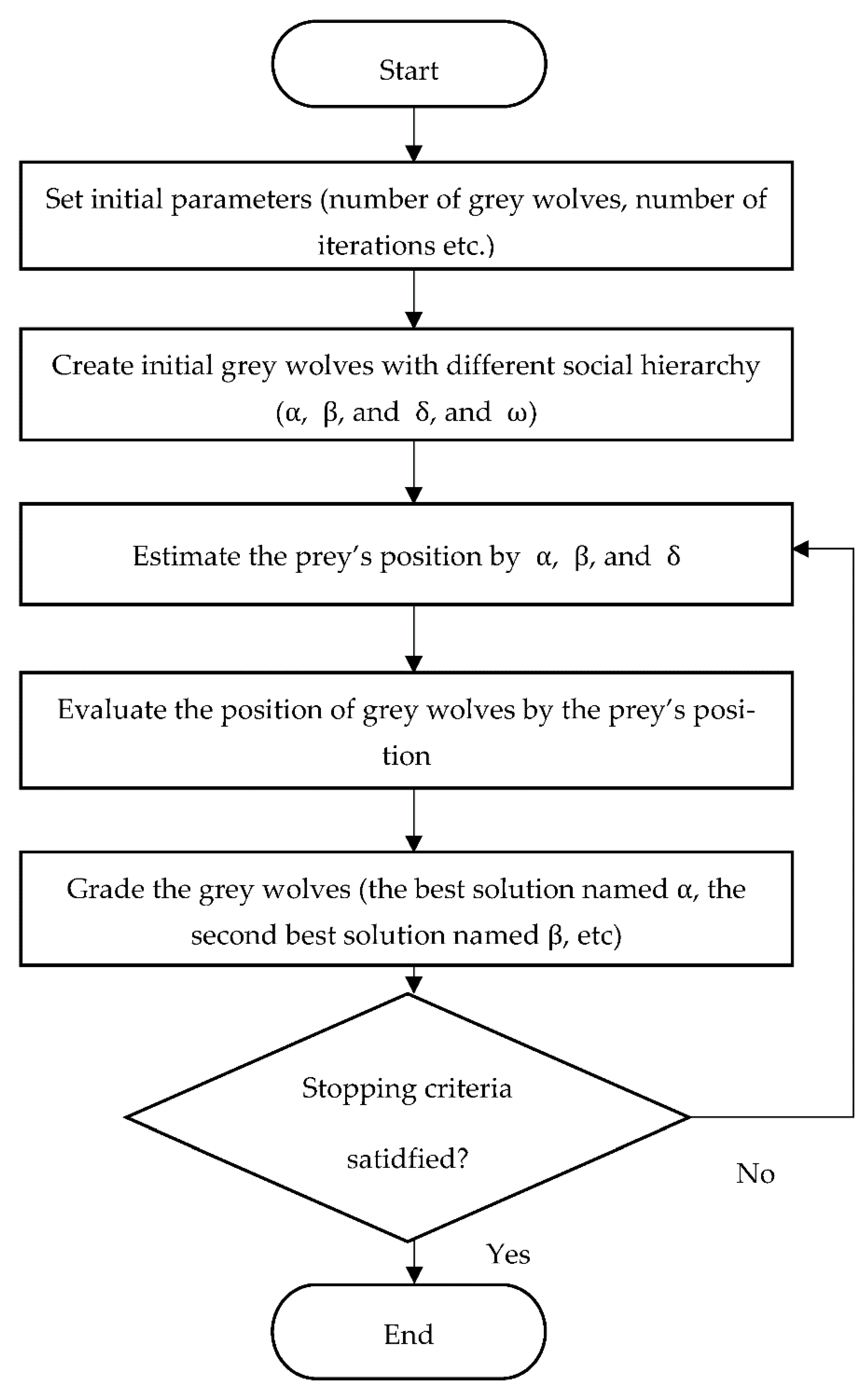
Figure 2.
Average monthly BDI from from January 2019 to August 2024.
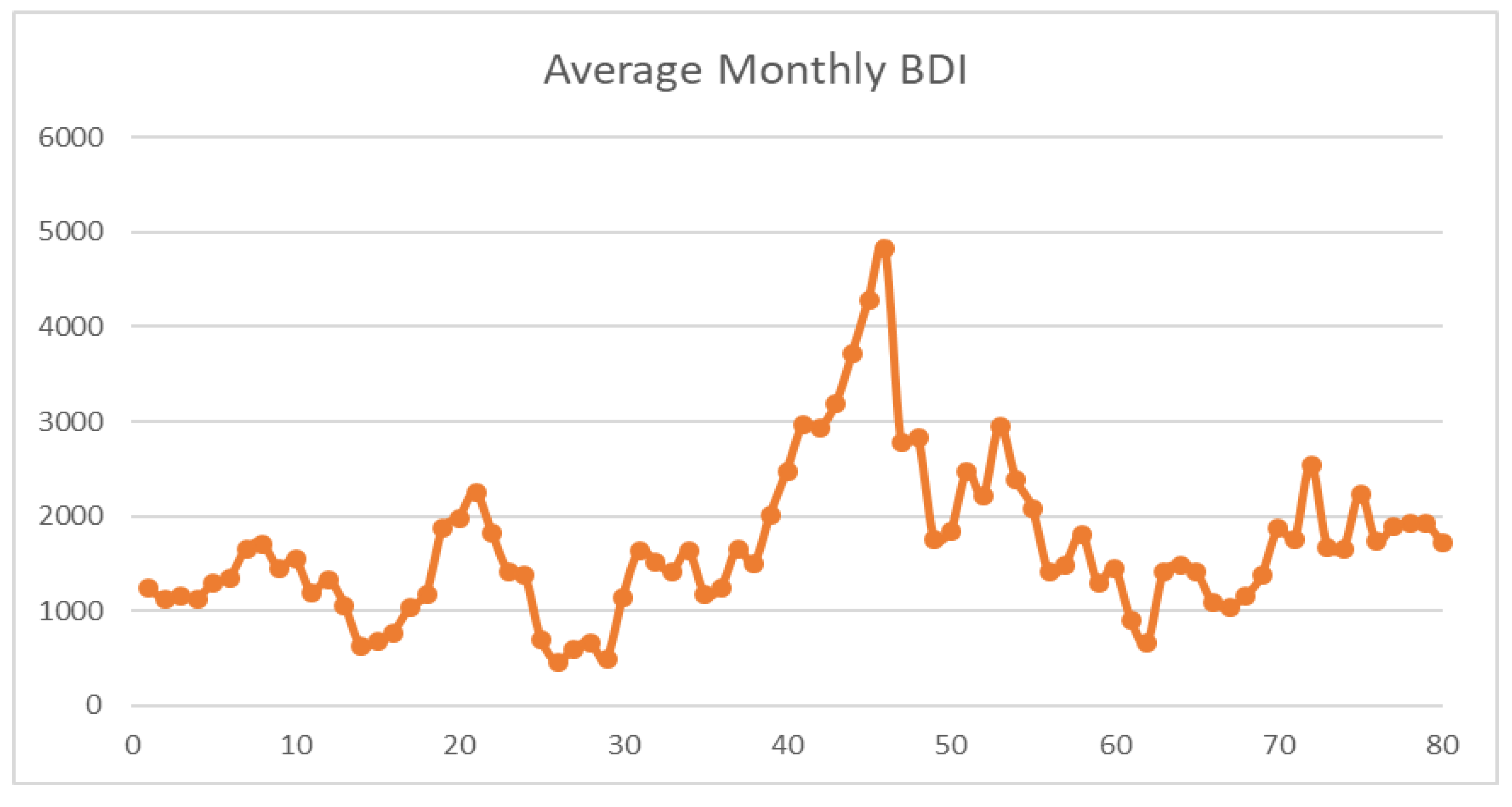
Figure 3.
The SAS output of average monthly BDI January 2019 to August 2024.
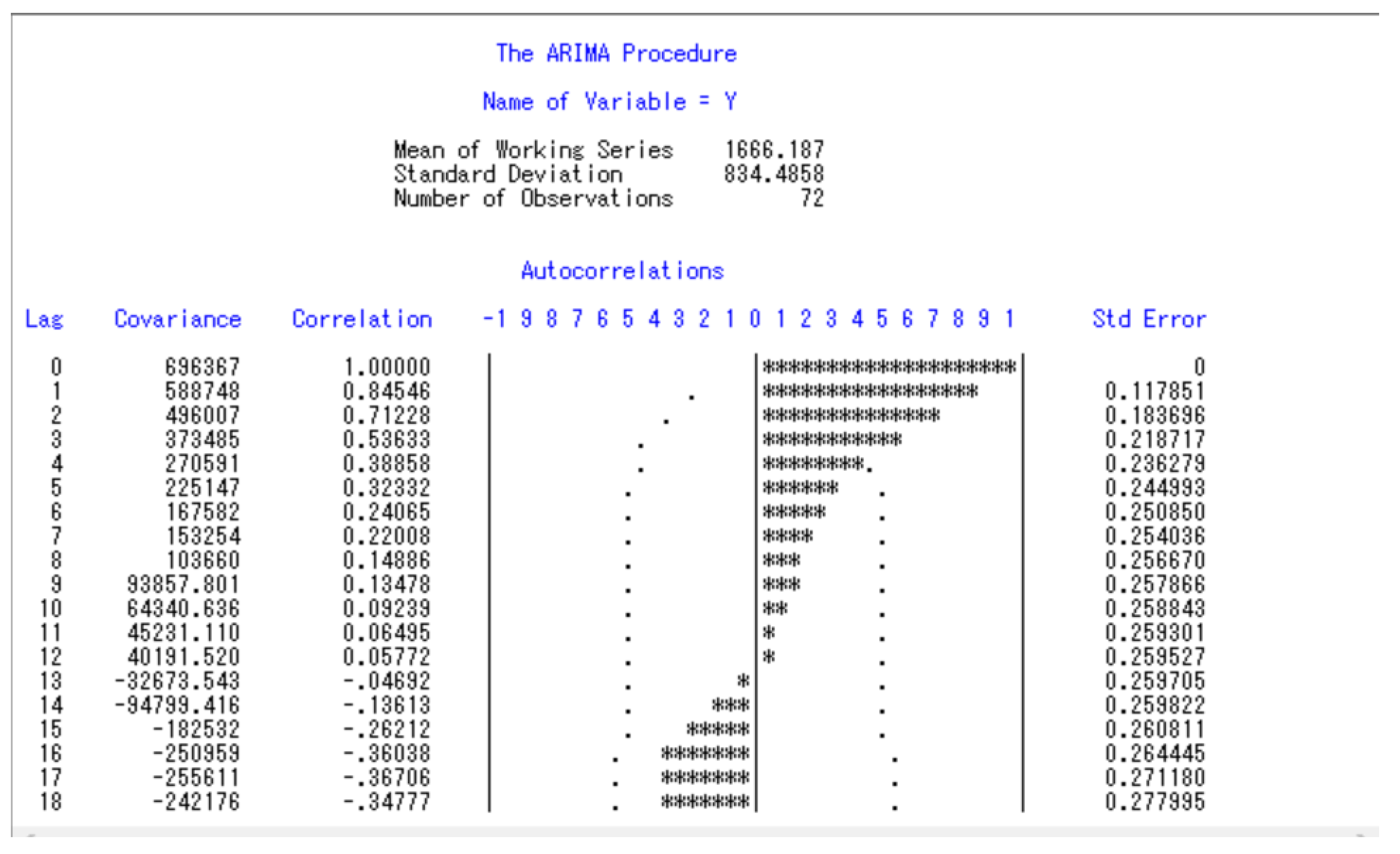
Figure 4.
The SAS output of the ACF for the first difference of the original data.
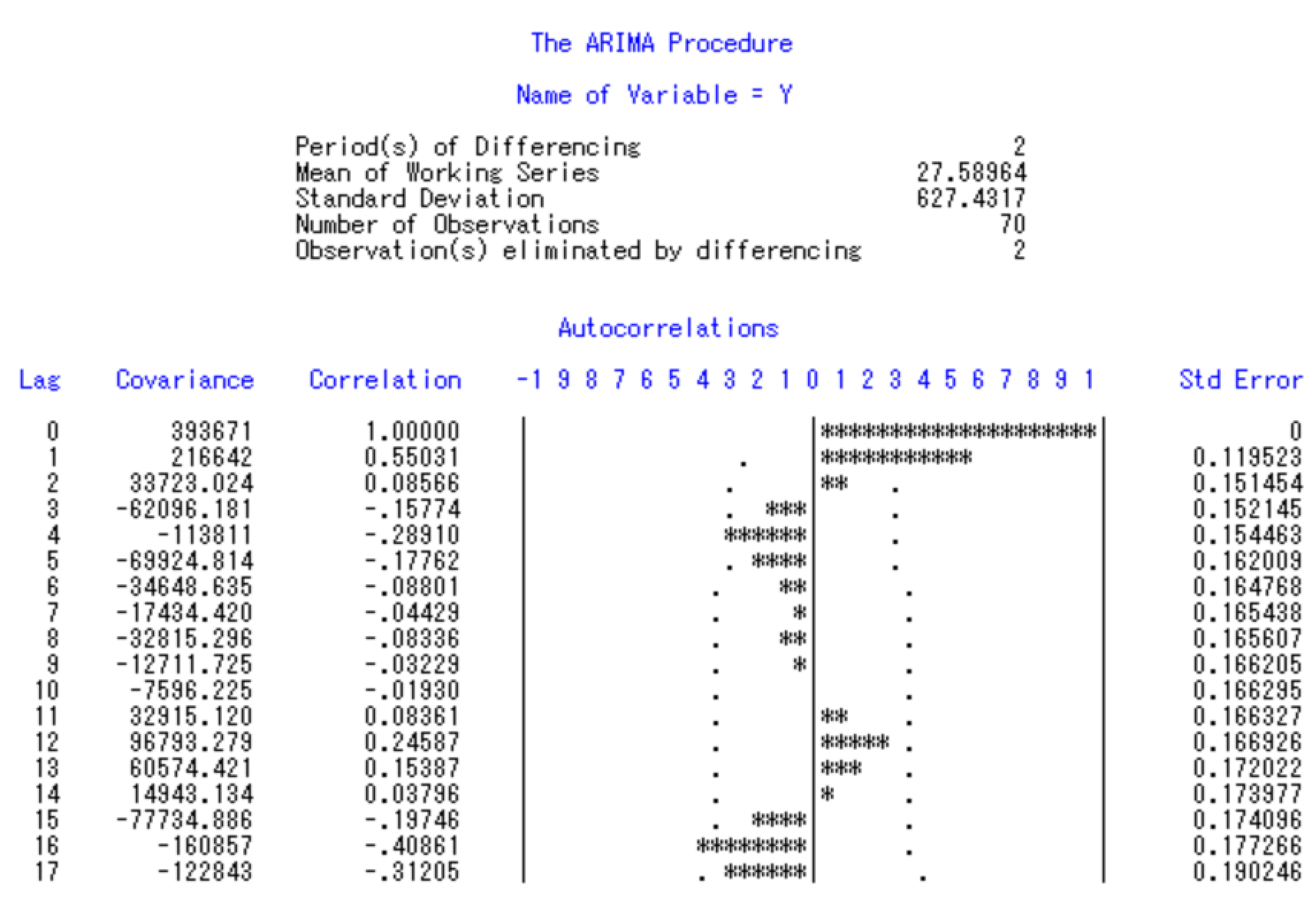
Figure 5.
The SAS output of the PACF for the first difference of the original data.
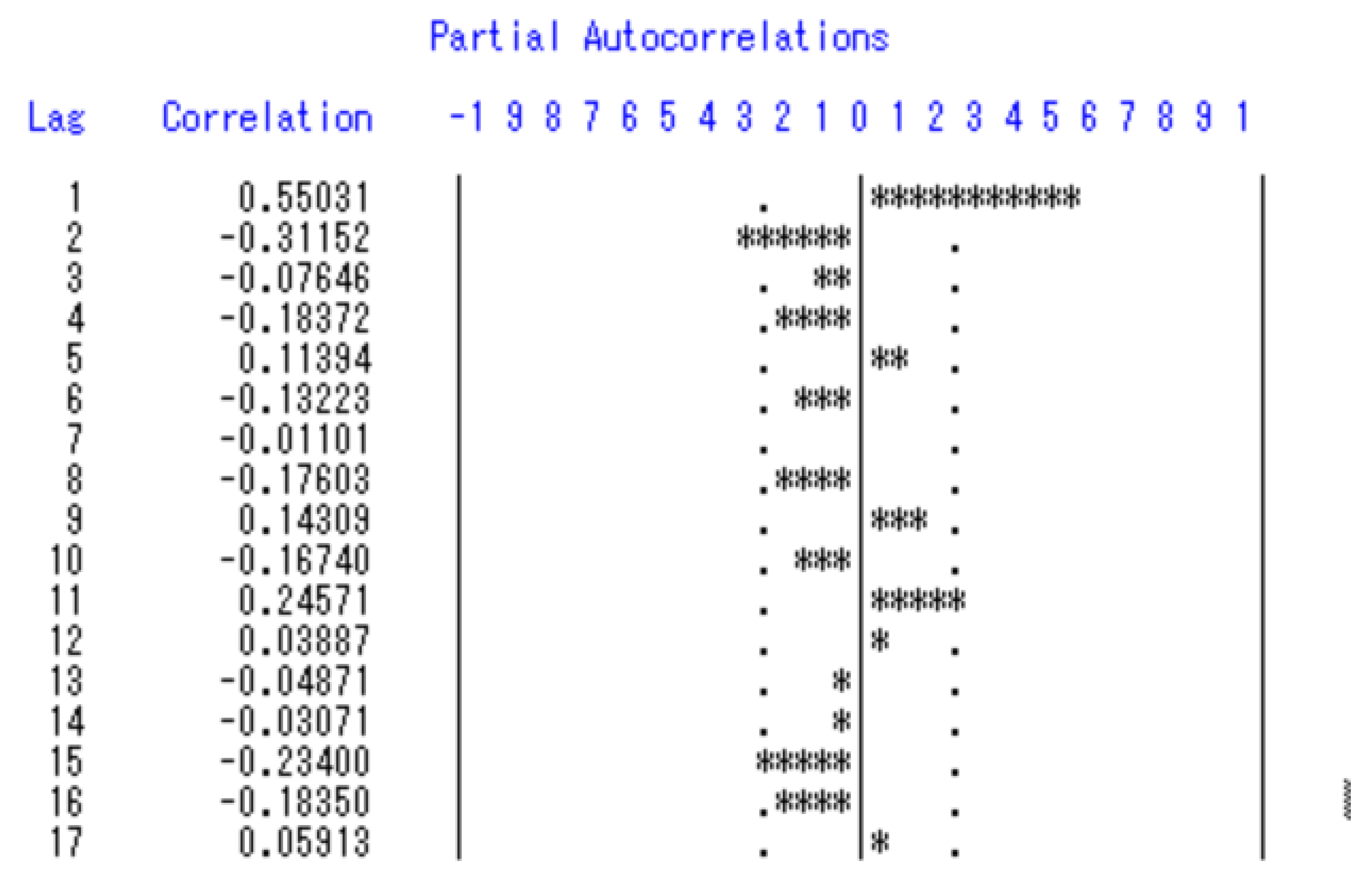
Figure 6.
Data composition results of BDI.

Table 1.
Average monthly BDI.
| Year | Month | BDI | Year | Month | BDI |
|---|---|---|---|---|---|
| 2019 | 1 | 1063.32 | 2022 | 1 | 1760.80 |
| 2019 | 2 | 628.75 | 2022 | 2 | 1834.90 |
| 2019 | 3 | 680.82 | 2022 | 3 | 2464.09 |
| 2019 | 4 | 773.25 | 2022 | 4 | 2220.37 |
| 2019 | 5 | 1037.05 | 2022 | 5 | 2943.05 |
| 2019 | 6 | 1174.40 | 2022 | 6 | 2389.45 |
| 2019 | 7 | 1869.74 | 2022 | 7 | 2078.48 |
| 2019 | 8 | 1981.86 | 2022 | 8 | 1412.36 |
| 2019 | 9 | 2256.41 | 2022 | 9 | 1487.14 |
| 2019 | 10 | 1827.61 | 2022 | 10 | 1814.67 |
| 2019 | 11 | 1419.29 | 2022 | 11 | 1298.95 |
| 2019 | 12 | 1380.71 | 2022 | 12 | 1453.41 |
| 2020 | 1 | 701.59 | 2023 | 1 | 908.81 |
| 2020 | 2 | 460.60 | 2023 | 2 | 658.35 |
| 2020 | 3 | 601.09 | 2023 | 3 | 1410.04 |
| 2020 | 4 | 663.90 | 2023 | 4 | 1480.33 |
| 2020 | 5 | 489.11 | 2023 | 5 | 1416.05 |
| 2020 | 6 | 1146.45 | 2023 | 6 | 1081.77 |
| 2020 | 7 | 1634.39 | 2023 | 7 | 1040.19 |
| 2020 | 8 | 1514.33 | 2023 | 8 | 1149.86 |
| 2020 | 9 | 1410.77 | 2023 | 9 | 1378.05 |
| 2020 | 10 | 1630.77 | 2023 | 10 | 1867.68 |
| 2020 | 11 | 1180.38 | 2023 | 11 | 1760.25 |
| 2020 | 12 | 1243.67 | 2023 | 12 | 2537.63 |
| 2021 | 1 | 1657.50 | 2024 | 1 | 1673.61 |
| 2021 | 2 | 1499.60 | 2024 | 2 | 1658.16 |
| 2021 | 3 | 2017.61 | 2024 | 3 | 2232.90 |
| 2021 | 4 | 2475.05 | 2024 | 4 | 1731.33 |
| 2021 | 5 | 2965.26 | 2024 | 5 | 1890.36 |
| 2021 | 6 | 2932.00 | 2024 | 6 | 1922.00 |
| 2021 | 7 | 3187.95 | 2024 | 7 | 1925.30 |
| 2021 | 8 | 3718.10 | 2024 | 8 | 1716.24 |
| 2021 | 9 | 4286.45 | |||
| 2021 | 10 | 4819.95 | |||
| 2021 | 11 | 2780.45 | |||
| 2021 | 12 | 2835.22 |
Source: Daily data is collected from https://data.eastmoney.com/cjsj/hyzs_EMI00107664.html; Monthly data is prepared by authors.
Table 2.
Class ratio test.
| 2023/10 | 2023/11 | 2023/12 |
|---|---|---|
| 0.4246 | 0.6484 | 0.6636 |
Table 3.
Accumulated generated sequence.
| 2023/9 | 2023/10 | 2023/11 | 2023/12 |
|---|---|---|---|
| 1378.05 | 3245.73 | 5005.98 | 7543.61 |
Table 4.
Mean value generating sequence.
| 2023/9~10 | 2023/10~11 | 2023/11~12 |
|---|---|---|
| 2311.89 | 4125.855 | 6274.795 |
Table 5.
A summary of the Q* values and prob-values for the models.
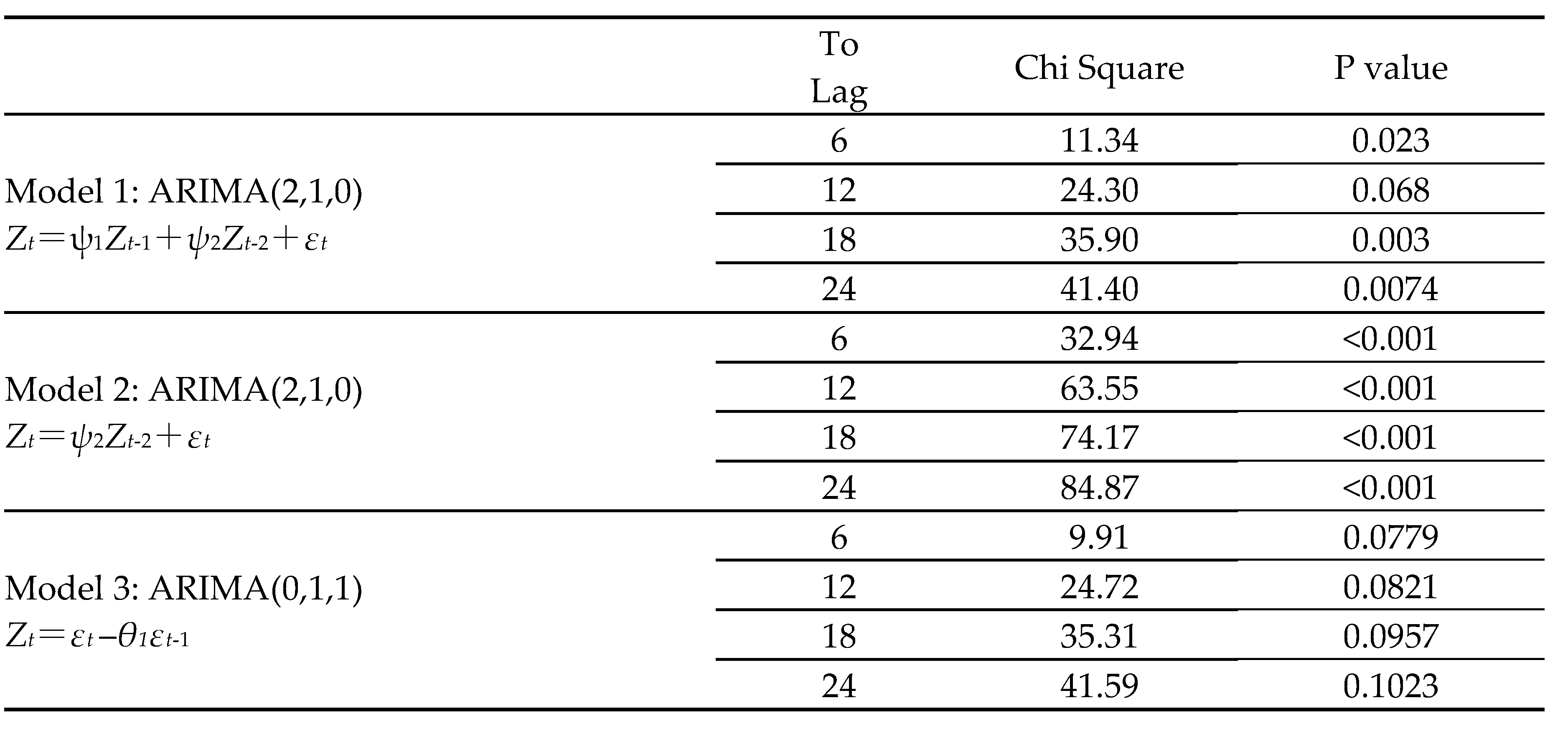 |
Table 6.
The best model found by auto_arima.
 |
Table 7.
The optimal weight for each IMF.
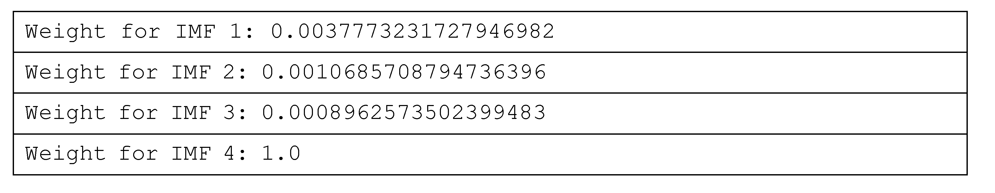 |
Table 9.
Performance of various methods of forecasting BDI.
| Accuracy measure | MAE | MAPE | RMSE | |
|---|---|---|---|---|
| Forecasting method | ||||
| Grey forecast | 500.561 | 27.2611 | 651.4161 | |
| ARIMA(1,0,0) | 245.875 | 14.2829 | 331.657 | |
| SVR | 295.301 | 15.3686 | 352.329 | |
| EMD-SVR-GWO | 151.977 | 8.3455 | 188.801 | |
Disclaimer/Publisher’s Note: The statements, opinions and data contained in all publications are solely those of the individual author(s) and contributor(s) and not of MDPI and/or the editor(s). MDPI and/or the editor(s) disclaim responsibility for any injury to people or property resulting from any ideas, methods, instructions or products referred to in the content. |
© 2025 by the authors. Licensee MDPI, Basel, Switzerland. This article is an open access article distributed under the terms and conditions of the Creative Commons Attribution (CC BY) license (http://creativecommons.org/licenses/by/4.0/).
Copyright: This open access article is published under a Creative Commons CC BY 4.0 license, which permit the free download, distribution, and reuse, provided that the author and preprint are cited in any reuse.


