
Submitted:
11 October 2025
Posted:
13 October 2025
You are already at the latest version
Abstract
We compare three modern Bayesian approaches, Hamiltonian Monte Carlo, Variational Bayes, and Integrated Nested Laplace Approximation, for two classic spatial econometric specifications: the spatial lag model and spatial error model. Our Monte Carlo experiments span a range of sample sizes and spatial neighborhood structures to assess accuracy and computational efficiency. Overall, posterior means exhibit minimal bias for most parameters, with precision improving as sample size grows. VB and INLA deliver substantial computational gains over HMC, with VB typically fastest at small and moderate samples and INLA showing excellent scalability at larger samples. However, INLA can be sensitive to dense spatial weight matrices, showing elevated bias and error dispersion for variance and some regression parameters. Two empirical illustrations underscore these findings: a municipal expenditure reaction function for Île-de-France and a hedonic price for housing in Ames, Iowa. Our results yield actionable guidance. HMC remains a gold standard for accuracy when computation permits; VB is a strong, scalable default; and INLA is attractive for large samples provided the weight matrix is not overly dense. These insights help practitioners select Bayesian tools aligned with data size, spatial neighborhood structure, and time constraints.
Keywords:
spatial econometrics
; Bayesian inference
; Hamiltonian Monte Carla
; variational bayes
; INLA
1. Introduction
In various real-world applications, researchers rely on geolocated data, which allow establishing connections between objects in space. Analyzing such spatial data poses certain challenges since classical regression models rely heavily on the independence assumption among observations that is often violated when spatial units are present. To address this issue, spatial econometric models have been developed to explicitly account for spatial dependence in the data (Besag, 1974; Whittle, 1954). Spatial dependence can arise either from spatial autocorrelation in the outcomes and/or determinants, which reflects similarities between geographically close observations, or from a spatially correlated error term, which is often caused by unobserved spatial heterogeneity, omitted variables or spatial scale mismatches. These two forms of spatial dependence give rise to two widely used model specifications, the spatial lag model (SLM) and the spatial error model (SEM) (Anselin, 1988).
Due to the presence of the endogenous lag term in SLMs and the non-spherical error term in SEMs, ordinary least squares estimators are typically biased and/or inefficient. To address this, researchers have developed various estimation techniques since the 1980s, including (quasi) maximum likelihood, generalized method of moments and spatial two-stage least squares estimators (Elhorst, 2014). These frequentist approaches have been extensively explored, but Bayesian methods took another decade to gain broader attention in spatial econometrics (LeSage, 1997).
The first papers in this area have mainly explored sampling-based Markov chain Monte Carlo (MCMC) methods for estimating spatial econometric models. LeSage (1997) introduced a variant of the Metropolis-Hastings algorithm for spatial econometric models, and LeSage and Pace (2009) provided a comprehensive treatment of spatial models estimated using MCMC methods. The MCMC method provides flexible yet computationally demanding solutions to estimate spatial econometric models. To overcome the high computational cost of MCMC methods, researchers have then employed techniques such as fast sparse matrix determinant calculation (Bivand et al., 2013) and advanced MCMC variants like griddy Gibbs and blocked Gibbs sampling (LeSage & Pace, 2009; Parent & LeSage, 2012).
Nowadays, the deepening understanding of Bayesian inference in statistics and econometrics, the growth of computational power and the development of dedicated software have led to the emergence of state-of-the-art, faster Bayesian methods. Among these, Hamiltonian Monte Carlo (HMC) (Betancourt et al., 2017), Variational Bayes (VB) (Blei et al., 2017), and Integrated Nested Laplace Approximation (INLA) (Bakka et al., 2018) stand out. Each of these methods is designed to reduce computational burden and make Bayesian estimation accessible to non-specialists.
First, HMC, a modern variant of MCMC, improves sampling efficiency by using gradient-based proposals. It also employs the No-U-Turn Sampler (NUTS) (Hoffman & Gelman, 2014), which adaptively chooses step sizes and the number of leapfrog iterations. Second, VB, including mean-field variational Bayes (MFVB) (Ormerod & Wand, 2010) and integrated non-factorized variational inference (INFVB) (Han et al., 2013), has emerged as a computationally faster alternative to MCMC for complex models (Wijayawardhana et al., 2025). Although its application to spatial econometric models remains limited, studies such as Wu (2018) and Bansal et al. (2021) have successfully applied VB to spatial autoregressive combined models and spatial count data models. Finally, INLA approximates posterior marginals using repeated Laplace approximations, offering a highly efficient method for latent Gaussian models, including certain spatial econometric models (Bivand et al., 2014). Unlike MCMC, which approximates joint posterior distributions, INLA directly computes approximations of marginal posteriors, reducing computational steps and often achieving results within a few minutes.
With the availability of these advanced Bayesian methods, practitioners may face uncertainty in determining which approach is most efficient or appropriate for a given research context. Some studies (Hubin & Storvik, 2016) have compared Bayesian methods but these efforts have largely focused on non-spatial models. Conversely, comprehensive comparative analyses of modern Bayesian techniques in spatial econometric models remain scarce (Taylor & Diggle, 2014). As such, this paper offers a systematic and comparative evaluation of these state-of-the-art Bayesian methods when applied specifically to the most used spatial econometric models like the spatial lag model (SLM) and spatial error model (SEM). To the best of our knowledge, no existing study has thoroughly assessed the performance trade-offs, such as estimation accuracy, computational efficiency, and robustness to different sample size and spatial structures among HMC, VB, and INLA in spatial settings. This study addresses that gap and aims to offer practical guidance for practitioners choosing among Bayesian tools in various spatial econometric applications.
The remainder of this paper is organized as follows: Section 2 introduces the SLM and SEM specifications. Section 3 presents the three Bayesian techniques under consideration. Section 4 details the simulation experiments and results. Section 5 discusses the simulation results and highlights their implications for methodological choices in spatial econometric modeling. Section 6 provides two empirical examples and Section 7 concludes with key findings.
2. Spatial Econometric Models
Among the various specifications of spatial econometric models, the SLM and SEM are the most widely used by practitioners1.
Let be the vector of response variable observed at spatial locations , X be the design matrix containing covariates, and be the spatial weight matrix that reflects the spatial connectivity structure between observations. The SLM is given by:
where denotes an identity matrix, and is a variance parameter. The vector contains the covariate parameters, and is the spatial autocorrelation parameter which measures the strength and the direction of spatial dependence. Regarding the spatial weight matrix , its entry is non-zero if unit is a neighbour of unit , and zero otherwise. The diagonal of matrix is then set to zero. The is commonly constructed to be sparse. In addition, it is common practice to perform row-normalization on (Harris et al., 2011).
Since SLMs include the endogenous term , it can be expressed as:
where the non-linear transformation is applied on both the covariate and error term. This model is often used to represent spatial peer effects, neighborhood diffusion or spillover effects, as in applications to technical innovation and fiscal federalism.
The SLM simplifies to the SEM when preceding the term in Equation 1 is set to 0. The SEM is given by:
or equivalently:
This model expresses spatial covariation in errors not accounted for by independent variables, measurement errors, and mismatch between the spatial units used and the scale at which the process occurs (Anselin & Bera, 1998).
For both the SLM and SEM, since the error vector is normally distributed, the response variable is multivariate Gaussian with the covariance matrix . To ensure the validity of as a proper covariance matrix, the parameter does not take on any of the values, but it restricts to the range2 in presence of a row-normalized .
Besides, the likelihood for both models writes:
with and for SEM and SLM, respectively.
To estimate these two models, the Bayesian approach requires prior assumptions on model parameters. Typically, it assumes prior independence between and other parameters but adopts a normal prior for that conditions on the sampled value of . Then, with an inverse Gamma prior on , we have:
For prior on , since spatial correlation is usually positive, a uniform prior on constrained to is often used (Lesage & Pace, 2009):
In this way, the full conditional density for reads:
and the full conditional density for reads:
with be an unknown constant.
3. Bayesian Estimation Procedures
Early formal developments in Bayesian estimation for linear models with spatial dependence can be traced back to works by Hepple (1979) and Anselin (1980). The introduction of the Gibbs sampler by Geman and Geman (1984) marked a turning point, making Bayesian methods more accessible due to its flexibility and ease of implementation. Gibbs sampling significantly simplified the estimation of classic spatial econometric models (Robert & Casella, 2011). However, it often comes with drawbacks such as long computation times, high resource demands, and difficulties in handling high-dimensional models3, especially those involving latent variables4.
With the advent of the big data era, spatial econometric models have become increasingly complex, often leveraging large datasets and intricate hierarchical structures. This growing complexity has driven the need for more advanced Bayesian computational methods. In response, a variety of solutions have emerged, ranging from simulation-based to optimization-based approaches. In this section, we focus on three such methods that have gained prominence for the last 10 years: Hamiltonian Monte Carlo, Variational Bayes, and Integrated Nested Laplace Approximation.
3.1. Hamiltonian Monte Carlo
Hamiltonian Monte Carlo (Neal, 2011), paired with the No-U-Turn Sampler (NUTS) (Hoffman & Gelman, 2014), is a simulation-based technique that draws on Hamiltonian dynamics to explore the posterior distribution efficiently. Although conceptually rooted in the broader class of MCMC methods, HMC is designed to overcome the inefficiencies of conventional random-walk Metropolis-Hastings schemes by leveraging both likelihood and gradient information to iteratively construct proposals that have a high probability of being accepted.
More precisely, HMC methods introduce auxiliary variables to record information about both the “position” of the sampler, corresponding to the parameters of interest, and the “momentum”, which guides how the sampler moves to achieve better proposals. The momentum variable is assumed to follow a multivariate normal distribution that does not depend on the parameter of interest (Betancourt, 2017).
The position variable and momentum variable together form a joint state, described by a Hamiltonian function representing the total energy of the system:
where denotes the potential energy and represents the kinetic energy.
To sample from this joint density, HMC simulates the evolution of the system using discrete-time approximations of Hamiltonian dynamics, most commonly the leapfrog integrator. This process updates both position and momentum variables in small steps (half-step updates of the momentum and full-step updates of the position) governed by a step size and a number of steps :
After simulating steps, the proposal is accepted or rejected using a standard Metropolis acceptance criterion. The acceptance rate is typically much higher for HMC than for classic samplers, since HMC trades simplicity in generating proposals for higher efficiency with those proposals.
Tuning parameters such as and is critical to performance. The NUTS algorithm dynamically selects these values to prevent inefficient exploration (i.e., U-turns in parameter space), enhancing convergence and reducing user intervention.
In summary, HMC greatly improves sampling efficiency by utilizing geometric information about the posterior distribution, but it remains a simulation-based method. In contrast, the next two methods, VB and INLA, rely on optimization rather than simulation to approximate posteriors, offering substantial computational advantages in many scenarios.
3.2. Variational Bayes
Variational Bayes, also known as Variational Inference, is an optimization-based technique for approximate Bayesian inference that has gained widespread adoption, particularly in the machine learning community (Beal, 2003).
The idea behind VB is to approximate the target posterior with a more manageable distribution , drawn from a variational family. The aim is to choose that is as close as possible to , where closeness is measured using the Kullback-Leibler (KL) divergence (Cover, 1999):
Where
Because the true posterior includes an intractable normalizing constant, KL divergence is typically minimized indirectly by maximizing the evidence lower bound (ELBO) (Fox & Roberts, 2012):
As a result, the KL divergence can be rewritten as
Maximizing the ELBO yields the best approximation within the variational family and provides a lower bound on the marginal likelihood, useful for model comparison.
Considering the mean-field5 variational inference (that we used in the following simulation study), the variational distribution is often assumed to follow a mean-field structure, i.e., the variation family over latent variables of are mutually independent. The joint density reads:
Then, Automatic Differentiation Variational Inference (ADVI) algorithm further streamlines this process. ADVI operates in three steps6: (1) transforming latent variables to an unconstrained space, (2) assuming a multivariate Gaussian form for , and (3) applying stochastic optimization using automatic differentiation to maximize the ELBO.
This is particularly important in two scenarios. First, when both and are high-dimensional, ranging from thousands to tens of thousands of parameters, VB can approximate within a reasonable computing time. Second, VB is especially well-suited for rapidly exploring multiple models. To summarize, VB leverages modern optimization techniques to minimize the “distance” between the variational posterior and the true posterior distribution.
3.3. Integrated Nested Laplace Approximation
INLA is another optimization-based approach, designed specifically for latent Gaussian models. Rather than sampling from the target posterior directly, INLA approximates marginal posterior distributions using a combination of Laplace approximations and low-dimensional numerical integration (Rue et al., 2009).
As its name suggests, the Laplace approximation is closely associated with Pierre-Simon Laplace, who, over two centuries ago, proposed a simple and practical method for computing general posterior expectations. Tierney and Kadane (1986) later revived and formalized this technique, establishing it as an asymptotic approximation for posterior expectations. Rue et al. (2009) extended this approach further by adapting it to approximate marginal posteriors in latent Gaussian models. By applying the Laplace approximation repeatedly and combining it with low-dimensional numerical integration, they developed the INLA approach. Although INLA is specifically designed for latent Gaussian models, this class includes a wide array of empirically relevant models, such as state-space models, spatial models, and spatiotemporal models.
In general, a latent Gaussian model can be expressed as:
where each observation is assumed to be independent, conditional on a linear predictor .
The full set of unknowns, denoted by , consists of an m-dimensional vector of hyperparameters , and the remaining unknowns dimensional latent variables. It is worth noting that the full set of unknowns are controlled by , where represents the precision matrix of the latent Gaussian field assumed for computational feasibility to be sparse. The goal is to obtain the marginal posteriors and . In latent Gaussian models, the number of hyperparameters is typically small, but the dimension of is large. In such cases, MCMC algorithms can be computationally prohibitive7. INLA addresses this challenge using a more efficient strategy, as outlined below.
INLA initially focuses on , since this component will be employed multiple times in calculating the marginal posterior of both hyperparameters and latent fields:
is approximated by
Here, the denominator represents a Gaussian approximation of , where is evaluated at the mode of for a given value of , and is the inverse of the Hessian of with respect to evaluated at . According to Rue et al. (2009), the Gaussian approximation is identical to the Laplace approximation of a marginal density.
Then, INLA concentrates on computing the marginal posterior for the -th element of , which is expressed as:
Here, INLA employs Laplace approximations again, yielding:
where represents the mode of at given values of and , with denoting all elements excluding the -th. Once is obtained, is computed using a deterministic numerical integration scheme defined over a grid of values for the low-dimensional .
Lastly, the marginal posterior for the -th element of is computed as:
This integral is computed using -dimensional deterministic integration over , once again assuming that is small. We refer to Gómez-Rubio et al. (2021) and Ling et al. (2025) for further details.
4. Monte Carlo Simulations
In this section, we evaluate the performance of HMC, VB, and INLA in estimating SLMs and SEMs through Monte Carlo simulation studies. Specifically, we aim to compare these methods in terms of both estimation accuracy and computational efficiency. To this end, we present and discuss a series of outputs derived from the simulations. We begin by outlining the data-generating process (DGP) and then focus on evaluating the accuracy of the posterior distributions for key model parameters, including the covariate coefficients, the variance parameter, and the spatial autoregressive parameters.
4.1. Simulation Designs
We conduct a series of Monte Carlo experiments to evaluate the estimation performance of HMC, VB, and INLA for SLMs and SEMs. Across all experiments, the DGPs are based on a fixed design matrix of dimension , where is a constant term and are two covariates. The covariate is drawn from a normal distribution , and is drawn from . The true coefficient vector is fixed at . We assume that the priors for the individual parameters are a priori independent. Besides, natural conjugate and noninformative priors are adopted, , and . The data are spatially structured over regular square lattice grids.
We design three simulation experiments to assess how the estimation accuracy and computational efficiency of the three Bayesian techniques respond to: (1) different sample sizes, (2) varying true values of key parameters, and (3) alternative spatial weight matrices. More precisely, in the first experiment, we vary the sample size across four levels: , and , while keeping the true values of parameters constant. In the second experiment, we examine the performance of the techniques to different true values of the spatial autocorrelation parameters () while keeping the sample size fixed at each of the four levels used in Experiment 1. Lastly, we assess the impact of different spatial weight matrix specifications. Here, the sample size is fixed at , which is typical in many empirical studies. In Experiments 1 and 2, the spatial weights matrix is defined using a rook contiguity criterion. In Experiment 3, we consider weights matrices based on the k-nearest neighbors (k-NN) and inverse distance with different truncation criteria, while keeping the true parameter values fixed at each of the three levels used in Experiment 2 to explore the impacts of non-symmetric and non-binary weight matrices. All experiments are repeated 300 times to ensure robustness of the results. For each experiment, we report average marginal posterior mean, the empirical bias (Bias), the empirical standard deviation (E-SD), root mean square error (RMSE) and mean absolute deviation (MAD) between the average marginal posterior mean and the true parameter values8.
Each experiment employs HMC with 2000 iterations following a burn-in period of 500 iterations. For VB, we adopt a mean-field variational family and use ADVI to approximate the posterior distribution by maximizing the ELBO within 10000 iterations. The INLA method is implemented using its standard framework, with the simplified Laplace approximation.
4.2. Simulation Results
Figure 1a,b present the simulations results for SLM models. Consistent with the detailed results provided in Table S1 (Online supplementary materials), all parameters of the SLMs are estimated with negligible bias across scenarios and estimation techniques. Across methods and parameters, estimation accuracy improves monotonically with sample size. In Figure 1a, the posterior distributions tighten and remain centered on the true values as sample sizes increase. In Figure 1b, both RMSE and MAD drop sharply from to and then gains become incremental. These trends are broadly robust to the level of spatial dependence.
Turning to method-specific behavior, HMC produces the most concentrated posteriors at small and moderate , with the posterior mean closely aligned to the true value for all parameters and all levels in Figure 1a. Consistent with this, HMC attains the lowest RMSE and MAD at small in Figure 1b. VB exhibits slightly wider spreads and small shifts at , most visible for and when , but its errors fall quickly. By , VB is practically indistinguishable from HMC. INLA, however, displays a persistent upward shift for the variance parameter across , yielding the largest RMSE and MAD for across different sample sizes. For the remaining parameters, however, INLA’s accuracy converges to the levels of HMC and VB as grows. This pattern may be attributed to INLA’s treatment of all components on the right-hand side of SLMs as random effects.
Considering parameters individually, the spatial autocorrelation coefficient is estimated well by all methods. Errors are small even at and display little sensitivity to different levels of (Figure 1a). The variance parameter is the most challenging for estimation. HMC and VB show mild overestimation only at and approach near-zero error by , whereas INLA’s upward bias persists across sample sizes. For the regression coefficients and , biases are small overall. INLA has a wider interquartile range (IQR) and a few outliers when , but the accuracy of all three methods improves steadily with increasing .
Overall, Figure 1 shows (i) minimal bias for most parameters and rapid variance reduction with increasing ; (ii) practical equivalence of HMC and VB once ; and (iii) a persistent positive bias of INLA for , alongside comparable accuracy to HMC and VB for and the regression coefficients at large .
by parameter and method for SLMs.
Figure 2a,b present the simulations results for SEM models. Overall, the results (see Table S2 of Online supplementary materials) show that parameter bias remains minimal, while precision and estimation accuracy consistently improve as sample size increases. The largest gains occur, from to , posteriors tighten markedly and both RMSE and MAD decline sharply. Beyond that, improvements are gradual. The same behavior holds across different levels of spatial dependence.
Method-specific differences are modest. HMC yields the most concentrated posteriors at small and moderate , especially for the regression coefficients. VB shows slightly wider IQR and small shifts at , especially for and , but the corresponding RMSE and MAD curves drop quickly. By , VB is practically indistinguishable from HMC. Unlike the SLM case, INLA does not exhibit a systematic upward bias for here. Its posteriors centers on the true values well across values, with both RMSE and MAD comparable to HMC and VB at small and moderate and often marginally lower at large and stronger spatial dependence.
Parameter-by-parameter, is estimated accurately by all methods. Both RMSE and MAD are small even at and weakly affected by dependence levels (top row of Figure 2a). The variance shows negligible bias at small , but its dispersion shrinks steadily and both RMSE and MAD approach zero by . For, biases are minor overall, a few outliers appear at , but all methods recover rapidly as grows.
In sum, Figure 2 indicates (i) minimal bias across parameters, (ii) rapid bias reduction with increasing sample size, and (iii) near-equivalence of HMC, VB, and INLA once , with INLA occasionally holding a slight edge at large .
by parameter and method for SEMs.
Table 1 reports simulation results using different spatial weight matrices. Unlike the earlier experiments that relied on a binary contiguity matrix, Experiment 3 employs denser spatial weight matrices, including both k-NN matrices and inverse-distance matrices. Specifically, , , and denotes k-NN matrices based on the 10, 20 and and 50 nearest neighbors, while and represents inverse-distance matrices truncated at 10 and 15 kilometers. Matrix sparsity is quantified using the index of Hoyer (2004): , with values of 0.895, 0.851, and 0.765 for k-NN matrices and 0.615, 0.502 for inverse-distance matrices. This decrease reflects increasing density of from Scenario 1 to Scenario 5. For comparison, the rook contiguity weight matrix used in Experiments 1 and 2 has a higher sparsity of 0.935. All spatial weight matrices are row-standardized, and simulations are conducted with a fixed sample size of and .
The upper panel of Table 3 shows results for SEMs. Across weight matrices, the bias in regression coefficients and variance estimates remains stable, with and consistently close to their true values. However, the autocorrelation parameter is more sensitive to matrix density. Under , its estimates decline to 0.459, 0.476, and 0.464 for HMC, VB, and INLA, respectively, further from the true value compared to the contiguity case. With the inverse-distance matrices, accuracy declines further. drops to 0.452, 0.475 and 0.462 under and remains biased under . This deterioration is reflected in RMSE, and MAD, which nearly doubles under and increases slightly further with the inverse-distance matrices.
A similar trend is observed for SLMs. HMC and VB remain robust across all weight matrices, with regression coefficient and variance estimates largely unaffected. Nonetheless, the accuracy of worsens as the matrices become denser, although the magnitude of the bias remains moderate. INLA, by contrast, is clearly more sensitive to sparsity. Similar to the previous simulations for SLMs, INLA still systemically overestimates the variance parameter. In addition, the bias of does increase marginally as the weight matrix becomes denser. We also notice that are significantly affected by the matrix sparseness. Specifically, under and , INLA produces substantial biases in and , along with inflated E-SD, RMSE, and MAD values. This inferior performance likely stems from INLA’s treatment of all right-hand-side components in SLMs as random effects, highlighting the need for caution when using INLA for dense matrices.
In summary, HMC and VB exhibit stable and reliable performance across alternative specifications of spatial weight matrices, INLA is more sensitive to matrix sparseness, especially for the variance parameter and regression coefficients. These findings partly support the idea of Mizruchi and Neuman (2008), where using sparse spatial weight matrices, such as binary contiguity or k-NN with fewer neighbors, is generally preferable for producing unbiased estimates. However, HMC and VB are more likely to be resistant to the dense weight matrices.
Figure 3 presents the computational time required to complete each simulation across different values of the spatial autocorrelation parameter, for both spatial models previously described9. Within each trellis panel, completion time per simulation is plotted as a function of the number of observations, holding other simulation parameters constant. The vertical axis is displayed on a logarithmic scale to facilitate comparison between HMC, VB, and INLA. All three methods exhibit approximately linear scaling with respect to the number of observations, resulting in straight lines with differing slopes.
For the SEM scenarios (top panels), HMC consistently requires more time than VB and INLA. Specifically, for smaller sample sizes (e.g., or ), all three methods complete a single simulation in under 10 seconds, but HMC remains the slowest, followed by INLA, with VB being the fastest. In this setting, VB is approximately 10 times faster than HMC, and INLA is about 5 times faster than HMC. This indicates that VB scales well for small datasets. As the sample size increases, HMC continues to exhibit the highest computational burden. For , INLA completes a simulation in approximately 11 seconds, compared to around 450 seconds for HMC. For the largest sample size (), INLA and VB require approximately 200 and 220 seconds, while HMC takes around 2000 seconds per simulation.
A similar pattern emerges in the SLM scenarios (bottom panels). VB continues to scale better than HMC as the sample size increases. However, INLA demonstrates the best scalability for large datasets in this case. For , INLA completes a simulation in as little as 2 seconds, compared to 220 seconds for VB and approximately 3100 seconds for HMC.
The computational burden associated with HMC stems from two main sources. First, the sparse numerical structures inherent to spatial econometric models are typically not exploited in HMC. As a result, although the gradient expressions produced are mathematically correct, they could be numerically inefficient to evaluate in the context of spatial models. Second, although HMC employs the NUTS, a sophisticated and adaptive algorithm designed for greater sampling efficiency, it still cannot fully compensate for the above-mentioned numerical inefficiencies. The observed differences in computational time between SLMs and SEMs, particularly for large sample sizes, may be attributed to model structure. In SLMs, all terms on the right-hand side are treated as random effects and incorporated into the linear predictor, which can significantly reduce computational loads. However, this simplification also introduces certain limitations, i.e., a trade-off between the larger variance parameter estimate () and computational time.
In summary, we would expect that the use of optimization-based Bayesian techniques greatly reduces computational time. For smaller datasets, HMC returns results within an acceptable time, but VB is more efficient here. INLA shows strong scalability, particularly in the SLM setting, where it outperforms both VB and HMC for moderate and large samples (see Figure 4).
5. Discussion
Across all simulation settings, we find that HMC, VB, and INLA produced posterior mean estimates with negligible bias for most model parameters. As sample size increases, the E-SD, RMSE, and MAD consistently decrease for all methods, reflecting improved estimation precision. This pattern holds across both SLMs and SEMs, and across various values of the spatial autocorrelation parameter indicating the robustness of these methods in terms of estimation accuracy. However, some notable differences emerged in small-sample contexts. VB exhibited a tendency to overestimate or underestimate when , though this bias diminishes rapidly as the sample size increases. INLA shows more persistent issues in small samples, particularly overestimating the variance parameter and producing higher RMSE and MAD values for covariates. These inaccuracies diminish as the sample size increases to 2500, but the small-sample performance gap between the optimization-based method and HMC is noteworthy.
Simulation results using denser spatial weight matrices reveal further differences in the robustness of the three Bayesian methods. Both HMC and VB maintain stable performance across all spatial weight structures, with acceptable variation in estimation bias or error metrics. This robustness underscores the reliability of these methods even when the spatial structure becomes more complex. In contrast, INLA shows notable sensitivity to the choice of spatial weight matrices. When using denser matrices such as , INLA exhibits increased bias in the estimates of , , and covariate coefficients. This is accompanied by larger values of E-SD, RMSE, and MAD. These findings indicate that INLA’s performance may deteriorate in contexts characterized by high spatial connectivity. Therefore, practitioners should apply INLA with caution under such conditions. One possible explanation for the bias with dense spatial matrices is that stronger spatial smoothing amplifies posterior uncertainty across all methods. Additionally, the higher bias exhibited by INLA in estimating SLMs under dense matrix settings may stem from the induced correlation between random effects. Specifically, since INLA treats both and as random effects, the assumption of independence between these components becomes problematic when dense spatial structures are introduced. These results align with the recommendation by Mizruchi and Neuman (2008) and are further supported by Smith (2009), who also highlighted the advantages of using sparse spatial weight matrices to improve estimation efficiency. Our findings reinforce this conclusion, particularly when using INLA.
The most pronounced differences among the three methods emerge in terms of computational time. VB and INLA significantly outperform HMC. For small sample sizes (), VB was the fastest method, typically completing each simulation in less than one to two seconds. INLA also demonstrates strong performance, with runtimes similarly within one to two seconds. In contrast, HMC is substantially slower, often requiring five to ten seconds per simulation even for small datasets. As sample size increases, the computational burden of HMC grows rapidly. For , HMC required approximately one hour per simulation, while VB and INLA remain around 200 seconds. Notably, INLA displays exceptional scalability in the SLM context.
The simulation study highlights key trade-offs across methods (see Table 2). HMC offers robust and accurate inference but at a high computational cost. VB is quite efficient and scales well but may experience small-sample bias, particularly in estimating spatial autocorrelation parameters. INLA provides a compelling alternative for large datasets, especially in SLMs, but may be sensitive to the spatial weight matrix structure and could overestimate variance components.
6. Empirical Applications
We consider two empirical applications, each relying on a single model specification, different levels of matrix sparsity, and sample sizes.
In the first case, we estimate a reaction function in which the expenditure of municipalities in Île-de-France, the French capital region, depends on the expenditures of their neighboring municipalities. Several mechanisms may yield such spatial interdependencies, including fiscal competition, yardstick competition, and Tiebout sorting (Agrawal et al., 2022). Empirical studies typically employ spatial lag models, where a positive spatial lag coefficient implies a mimicking strategy, while a negative one indicates a complementary strategy.
To explore this, we use data on the expenditure of 1280 municipalities for the year 2011. We estimate three empirical models with different dependent variables, current, capital and total expenditures (in €/capita), and a set of socio-economic control variables, including the share of active population (ACTPOP), the share of highly educated population (SUP), the logarithm of the share of individuals aged 0-10 (lPOP0010), aged 11-17 (lPOP1117), aged 18-24 (lPOP1824) and aged 65 and over years (lPOP64p). The neighborhood structure is defined by an inverse-distance weight matrix truncated at 25 kilometers, yielding a relatively dense specification with a sparsity index of 0.72. Our primary focus is on estimating the spatial lag coefficient, we also report the estimation results for the other regression coefficients.
Given the sample size and the specification of the weight matrix, we employ the VB approach for model estimation, but with 20000 iterations to guarantee ELBO convergence. The corresponding estimation results are reported in Table 3. The estimation results indicate that the spatial lag coefficient is consistently positive across current, capital, and total expenditures. This suggests that, overall, municipalities in Île-de-France pursued a mimicking strategy in their spending behavior in 2011. Furthermore, the spatial autocorrelation coefficients are smaller in magnitude for capital expenditure compared to current expenditure, highlighting the more discretionary character of capital spending.

Table 3.
VB estimation of the SLM for municipal expenditures in 2011.
| Variable | Current expenditure | Capital expenditure | Total expenditure | ||||||
| Mean | 95%CIs | Mean | 95%CIs | Mean | 95%CIs | ||||
| ACTPOP | -0.018 | (-0.024; -0.013) | -0.005 | (-0.019; 0.01) | -0.012 | (-0.02: -0.006) | |||
| SUP | 0.001 | (-0.001; 0.003) | -0.002 | (-0.006; 0.003) | 0.002 | (-0.001; 0.004) | |||
| lPOP0010 | 0.138 | (0.024; 0.254) | 0.06 | (-0.238; 0.362) | 0.063 | (-0.081; 0.211) | |||
| lPOP1117 | -0.282 | (-0.395; -0.178) | -0.285 | (-0.539; -0.041) | -0.333 | (-0.476; -0.202) | |||
| lPOP1824 | 0.236 | (0.156; 0.314) | 0.373 | (0.182; 0.56) | 0.264 | (0.164; 0.362) | |||
| lPOP64p | -0.023 | (-0.083; 0.039) | -0.143 | (-0.305; 0.016) | -0.112 | (-0.186; -0.035) | |||
| Spatial lag () | 0.928 | (0.925; 0.931) | 0.799 | (0.793; 0.805) | 0.866 | (0.863; 0.869) | |||
| Sigma () | 0.301 | (0.288; 0.314) | 0.788 | (0.756; 0.82) | 0.378 | (0.362; 0.395) | |||
| Computing time (s) | 467 | 177 | 467 | ||||||
Note: CIs stands for credible intervals.
In the second case, we estimate a hedonic price function for housing data which are inherently spatial. As previously stated, a SEM applied to hedonic housing prices can account for spatial autocorrelation in the error term, recognizing that the price at any given location depends not only on local property characteristics but also on unobserved, omitted characteristics from neighboring locations. Compared to traditional OLS-based hedonic models, the SEM typically yields more accurate and reliable estimates of housing prices (Bhattacharjee et al., 2012).
Here, we use the Ames dataset (available in the AmesHousing R-package), which contains information on 2777 properties10 in Ames, Iowa, USA. The dependent variable in the SEM is the logarithm of sale price. Explanatory variables include the logarithm of lot size (lnLot_Area), basement area (lnTotal_Bsmt_SF), and above-ground living area (lnGr_Liv_Area), along with garage size (Garage_Cars) and the number of fireplaces (Fireplaces). The spatial neighbourhood structure is represented by a k-NN weight matrix with 5 neighbors, producing a sparse specification with a sparsity index of 0.954. Given the sample size and the specification of the weight matrix, we employ the INLA approach to estimate this model. The corresponding estimation results are reported in Table 4.
The estimation results indicate that the spatial error coefficient is rather high (posterior mean value 0.683) and statistically significant. Furthermore, the regression coefficients are all positive and significant, indicating all these variables positively contribute to housing prices.
7. Conclusions
This study systematically compares the performance of three Bayesian estimation methods, Hamiltonian Monte Carlo, Variational Bayes, and Integrated Nested Laplace Approximation, for estimating parameters in spatial lag models and spatial error models. While previous literature has focused either on classical estimation approaches for spatial econometric models or on Bayesian techniques applied to non-spatial regression models, this study is the first to comprehensively review and evaluate state-of-the-art Bayesian methods specifically tailored to spatial econometric models. In doing so, we uncover several novel findings not previously documented in the literature.
Our results suggest that no single method dominates across all criteria of interest. Each method exhibits distinct advantages and limitations in terms of computational efficiency, estimation accuracy, and sensitivity to model specifications as well as configurations. HMC delivers robust and flexible inference, making it suitable for small datasets or settings where full posterior exploration is critical, despite its relatively high computational cost. VB and INLA, by contrast, are far more computationally efficient and scale well to larger datasets. INLA, in particular, demonstrates excellent scalability in SLMs, but its estimation accuracy may degrade in the presence of dense spatial weight matrices or small sample sizes. In such cases, VB offers a more robust alternative, though potentially at a higher computational cost compared to INLA.
These findings imply that Bayesian method selection in spatial econometrics should be driven by practical considerations, including sample size, model complexity, spatial connectivity structures, and computational resources. VB and INLA are highly attractive for large-scale applications, but careful attention must be paid to the choice of spatial weight matrices, especially for INLA, which is more sensitive to the sparseness of spatial weight matrices.
Future research could explore adaptive strategies that integrate the strengths of these methods. For instance, enhancing the NUTS sampler with sparse matrix-aware algorithms (Wolf et al., 2018), such as sparse Cholesky or LU decomposition, could substantially improve the computational efficiency of HMC for spatial econometric models. Likewise, extending INLA by embedding it within an HMC sampling framework (Berild et al., 2022) may enhance its accuracy in small-sample contexts or when handling dense spatial connectivity structures. In addition, further investigation is needed to assess the robustness of Bayesian approaches, particularly INLA, to heteroskedasticity in the error structure. Finally, expanding simulation experiments to include spatial panel models would offer valuable insights for methodological development and practical application in spatial econometrics.
Supplementary Materials
The following supporting information can be downloaded at the website of this paper posted on Preprints.org, Figure S1: title; Table S1: title; Video S1: title.
Author Contributions
For research articles with several authors, a short paragraph specifying their individual contributions must be provided. The following statements should be used “Conceptualization, Y.L. and J.L.G.; methodology, Y.L.; software, Y.L.; validation, Y.L. and J.L.G.; formal analysis, Y.L.; investigation, Y.L.; resources, Y.L. and J.L.G.; data curation, , Y.L. and J.L.G.; writing—original draft preparation, Y.L.; writing—review and editing, Y.L. and J.L.G.; visualization, Y.L. and J.L.G.; supervision, Y.L. and J.L.G.; project administration, Y.L. and J.L.G.; funding acquisition, Y.L. All authors have read and agreed to the published version of the manuscript.”.
Funding
Please add: “This research was funded by National Natural Science Foundation of China, grant number 42501311 and Hainan Provincial Natural Science Foundation of China, grant number 225QN296”.
Data Availability Statement
The data are available upon request from the authors.
Acknowledgments
The authors have reviewed and edited the output and take full responsibility for the content of this publication.
Conflicts of Interest
The authors declare no conflict of interest.
| 1 | For a comprehensive introduction to various spatial econometric models and their estimation, see Elhorst (2014) and, more recently, the sections devoted in the analysis of spatial data in Fisher and Nijkamp (2021) and Nijkamp et al. (2025). |
| 2 |
is the minimum eigenvalues of . |
| 3 | The so-called “intractable” Bayesian problems typically include: (1) a data generating process that cannot readily be expressed as a probability density or mass function (the “unavailable likelihood” problem); (2) a high-dimensional parameter space (the “high dimensional” problem); and/or (3) a very large volume of observations (the “big-data” problem). |
| 4 | “Latent variables” denote unobserved random variables that form the underlying structure of the observed data. They are described as latent because they are not directly observable but are inferred indirectly through a probabilistic model. These variables typically represent spatial, temporal, or hierarchical random effects, serving as the “hidden layer” that links the observed data to the underlying model structure. |
| 5 | Originating from mean-field theory (Barabási et al., 1999), the mean field approximation assumes full independence among all latent variables given. |
| 6 | See Zhang et al. (2018) for all details on ADVI. |
| 7 | This is the fact that the scale of the unknowns (and potentially also) and the challenging geometry of the posterior. |
| 8 | Coverage probability is not reported, as all three Bayesian methods provide reliable point estimates; only in rare cases (2–3 instances) do VB and INLA underperform, while HMC remains consistently stable. |
| 9 | All simulations are conducted on a PC equipped with 16 cores and 64 GB of RAM. |
| 10 | The Ames dataset originally contains 2930 observations. After the data cleaning process, 2777 observations remain for analysis. |
References
- Agrawal, D. R., Hoyt, W. H., & Wilson, J. D. (2022). Local policy choice: theory and empirics. Journal of Economic Literature, 60(4), 1378–1455. [CrossRef]
- Anselin, L. (1980). Estimation Methods for Spatial Autoregressive Structures: A Study in Spatial Econometrics. Program in Urban and Regional Studies, Cornell University. https://books.google.com/books?id=JnpFAAAAYAAJ.
- Anselin, L. (1988). Spatial Econometrics: Methods and Models. In Operational Regional Science Series (Vol. 4). Springer. Netherlands. [CrossRef]
- Anselin, L., & Bera, A. K. (1998). Spatial dependence in linear regression models with an introduction to spatial econometrics. Statistics Textbooks and Monographs, 155, 237–290.
- Bakka, H., Rue, H., Fuglstad, G.-A., Riebler, A., Bolin, D., Illian, J., Krainski, E., Simpson, D., & Lindgren, F. (2018). Spatial modeling with R-INLA: A review. WIREs Computational Statistics, 10(6), e1443. [CrossRef]
- Bansal, P., Krueger, R., & Graham, D. J. (2021). Fast Bayesian estimation of spatial count data models. Computational Statistics & Data Analysis, 157, 107152. [CrossRef]
- Barabási, A.-L., Albert, R., & Jeong, H. (1999). Mean-field theory for scale-free random networks. Physica A: Statistical Mechanics and Its Applications, 272(1), 173–187. [CrossRef]
- Beal, M. J. (2003). Variational algorithms for approximate Bayesian inference. University of London, University College London (United Kingdom).
- Berild, M. O., Martino, S., Gómez-Rubio, V., & Rue, H. (2022). Importance sampling with the integrated nested Laplace approximation. Journal of Computational and Graphical Statistics, 31(4), 1225–1237. [CrossRef]
- Besag, J. (1974). Spatial interaction and the statistical analysis of lattice systems (with discussion). Journal of the Royal Statistical Society Series B, 36, 192–236.
- Betancourt, M. (2017). A conceptual introduction to Hamiltonian Monte Carlo. ArXiv Preprint ArXiv:1701.02434.
- Betancourt, M., Byrne, S., Livingstone, S., & Girolami, M. (2017). The geometric foundations of Hamiltonian Monte Carlo. Bernoulli, 23(4A), 2257–2298. [CrossRef]
- Bhattacharjee, A., Castro, E., & Marques, J. (2012). Spatial Interactions in Hedonic Pricing Models: The Urban Housing Market of Aveiro, Portugal. Spatial Economic Analysis, 7(1), 133–167. [CrossRef]
- Bivand, R., Gómez-Rubio, V., & Rue, H. (2014). Approximate Bayesian inference for spatial econometrics models. Spatial Statistics, 9, 146–165. [CrossRef]
- Bivand, R., Hauke, J., & Kossowski, T. (2013). Computing the Jacobian in Gaussian Spatial Autoregressive Models: An Illustrated Comparison of Available Methods. Geographical Analysis, 45(2), 150–179. [CrossRef]
- Blei, D. M., Kucukelbir, A., & McAuliffe, J. D. (2017). Variational Inference: A Review for Statisticians. Journal of the American Statistical Association, 112(518), 859–877. [CrossRef]
- Cover, T. M. (1999). Elements of information theory. John Wiley & Sons.
- Elhorst, J. P. (2014). Spatial econometrics: from cross-sectional data to spatial panels (Vol. 479). Springer. Netherlands.
- Fischer, M., & Nijkamp, P. (2021). Handbook of Regional Science. Springer.
- Fox, C. W., & Roberts, S. J. (2012). A tutorial on variational Bayesian inference. Artificial Intelligence Review, 38(2), 85–95. [CrossRef]
- Geman, S., & Geman, D. (1984). Stochastic relaxation, Gibbs distributions, and the Bayesian restoration of images. IEEE Transactions on Pattern Analysis and Machine Intelligence, 6, 721–741.
- Gómez-Rubio, V., Bivand, R. S., & Rue, H. (2021). Estimating spatial econometrics models with integrated nested Laplace approximation. Mathematics, 9(17), 2044. [CrossRef]
- Han, S., Liao, X., & Carin, L. (2013). Integrated non-factorized variational inference. Advances in Neural Information Processing Systems, 26.
- Harris, R., Moffat, J., & Kravtsova, V. (2011). In search of ‘W.’ Spatial Economic Analysis, 6(3), 249–270.
- Hepple, L. W. (1979). Bayesian analysis of the linear model with spatial dependence. In Exploratory and explanatory statistical analysis of spatial data (pp. 179–199).
- Hoffman, M. D., & Gelman, A. (2014). The No-U-Turn sampler: adaptively setting path lengths in Hamiltonian Monte Carlo. J. Mach. Learn. Res., 15(1), 1593–1623. [CrossRef]
- Hoyer, P. O. (2004). Non-negative matrix factorization with sparseness constraints. Journal of Machine Learning Research, 5(9).
- Hubin, A., & Storvik, G. (2016). Estimating the marginal likelihood with Integrated nested Laplace approximation (INLA). ArXiv Preprint ArXiv:1611.01450.
- LeSage, J. P. (1997). Bayesian estimation of spatial autoregressive models. International Regional Science Review, 20(1–2), 113–129. [CrossRef]
- Lesage, J. P., & Pace, K. (2009). Bayesian Spatial Econometric Models. In Introduction to Spatial Econometrics (pp. 123–153).
- LeSage, J., & Pace, R. K. (2009). Introduction to spatial econometrics. Chapman and Hall/CRC.
- Ling, Y., Bai, K., & Yang, Y. (2025). Estimation of spatial panel data models with random effects using Laplace approximation methods. Spatial Economic Analysis, 1–22. [CrossRef]
- Mizruchi, M. S., & Neuman, E. J. (2008). The effect of density on the level of bias in the network autocorrelation model. Social Networks, 30(3), 190–200. [CrossRef]
- Neal, R. M. (2011). MCMC using Hamiltonian dynamics. Handbook of Markov Chain Monte Carlo, 2(11), 2.
- Nijkamp, P., Kourtit, K., Haynes, K. E., & Elburz, Z. (2025). Thematic Encyclopedia of Regional Science. Edward Elgar Publishing.
- Ormerod, J. T., & Wand, M. P. (2010). Explaining variational approximations. The American Statistician, 64(2), 140–153.
- Parent, O., & LeSage, J. P. (2012). Spatial dynamic panel data models with random effects. Regional Science and Urban Economics, 42(4), 727–738. [CrossRef]
- Robert, C., & Casella, G. (2011). A Short History of Markov Chain Monte Carlo: Subjective Recollections from Incomplete Data. Statistical Science, 26(1), 102–115. [CrossRef]
- Rue, H., Martino, S., & Chopin, N. (2009). Approximate Bayesian inference for latent Gaussian models by using integrated nested Laplace approximations. Journal of the Royal Statistical Society. Series B: Statistical Methodology, 71(2), 319–392. [CrossRef]
- Smith, T. E. (2009). Estimation Bias in Spatial Models with Strongly Connected Weight Matrices. Geographical Analysis, 41(3), 307–332. [CrossRef]
- Taylor, B. M., & Diggle, P. J. (2014). INLA or MCMC? A tutorial and comparative evaluation for spatial prediction in log-Gaussian Cox processes. Journal of Statistical Computation and Simulation, 84(10), 2266–2284. [CrossRef]
- Tierney, L., & Kadane, J. B. (1986). Accurate approximations for posterior moments and marginal densities. Journal of the American Statistical Association, 81(393), 82–86.
- Whittle, P. (1954). On stationary processes in the plane. Biometrika, 434–449.
- Wijayawardhana, A., Gunawan, D., & Suesse, T. (2025). Variational Bayes inference for simultaneous autoregressive models with missing data. Statistics and Computing, 35(3), 68. [CrossRef]
- Wolf, L. J., Anselin, L., & Arribas-Bel, D. (2018). Stochastic efficiency of Bayesian Markov chain Monte Carlo in spatial econometric models: an empirical comparison of exact sampling methods. Geographical Analysis, 50(1), 97–119. [CrossRef]
- Wu, G. (2018). Fast and scalable variational Bayes estimation of spatial econometric models for Gaussian data. Spatial Statistics, 24, 32–53. [CrossRef]
Figure 1.
(a) Posterior distributions by parameter for SLMs under varying sample sizes and spatial autocorrelation level. (b). RMSE and MAD vs.
Figure 1.
(a) Posterior distributions by parameter for SLMs under varying sample sizes and spatial autocorrelation level. (b). RMSE and MAD vs.
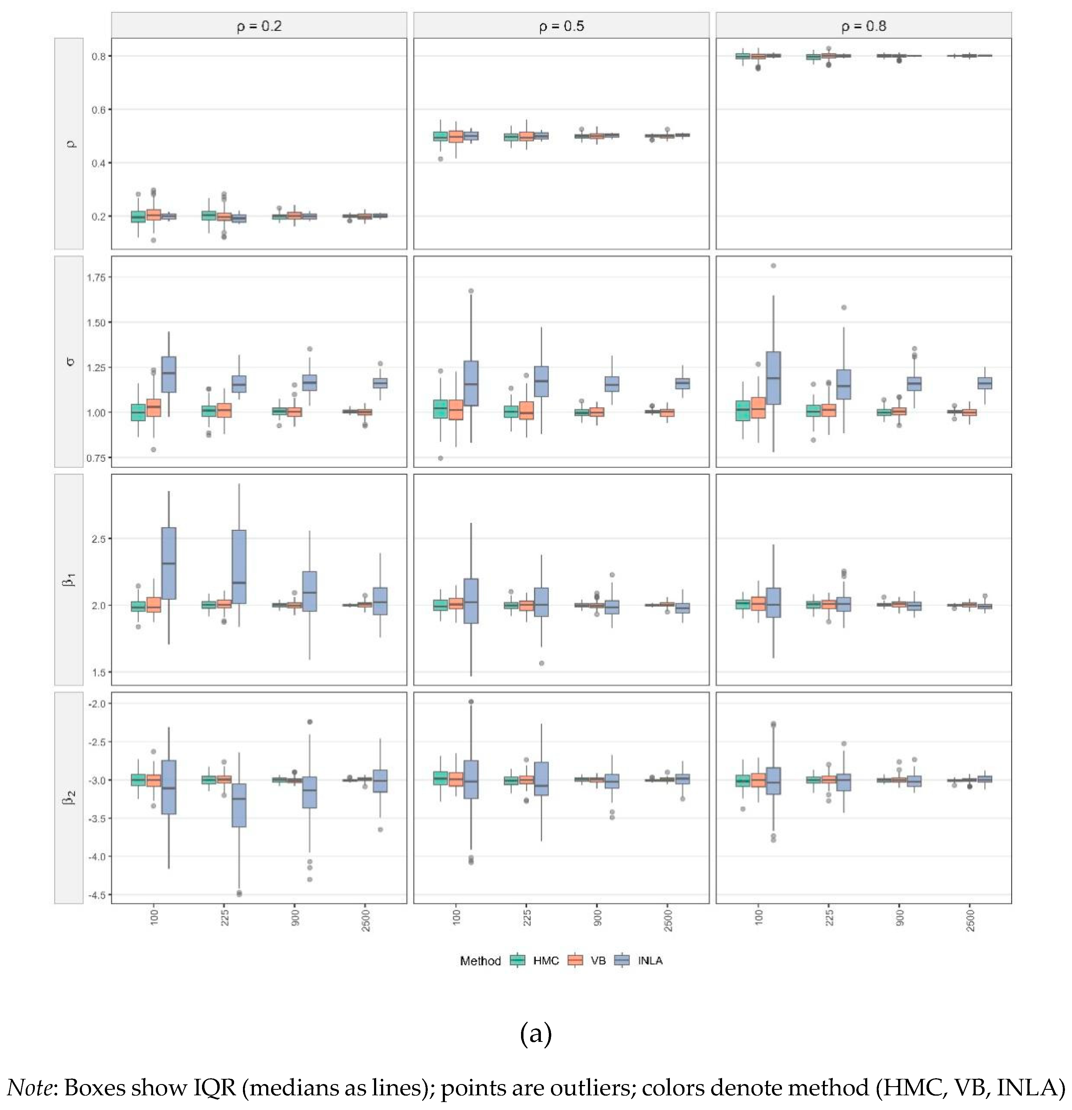
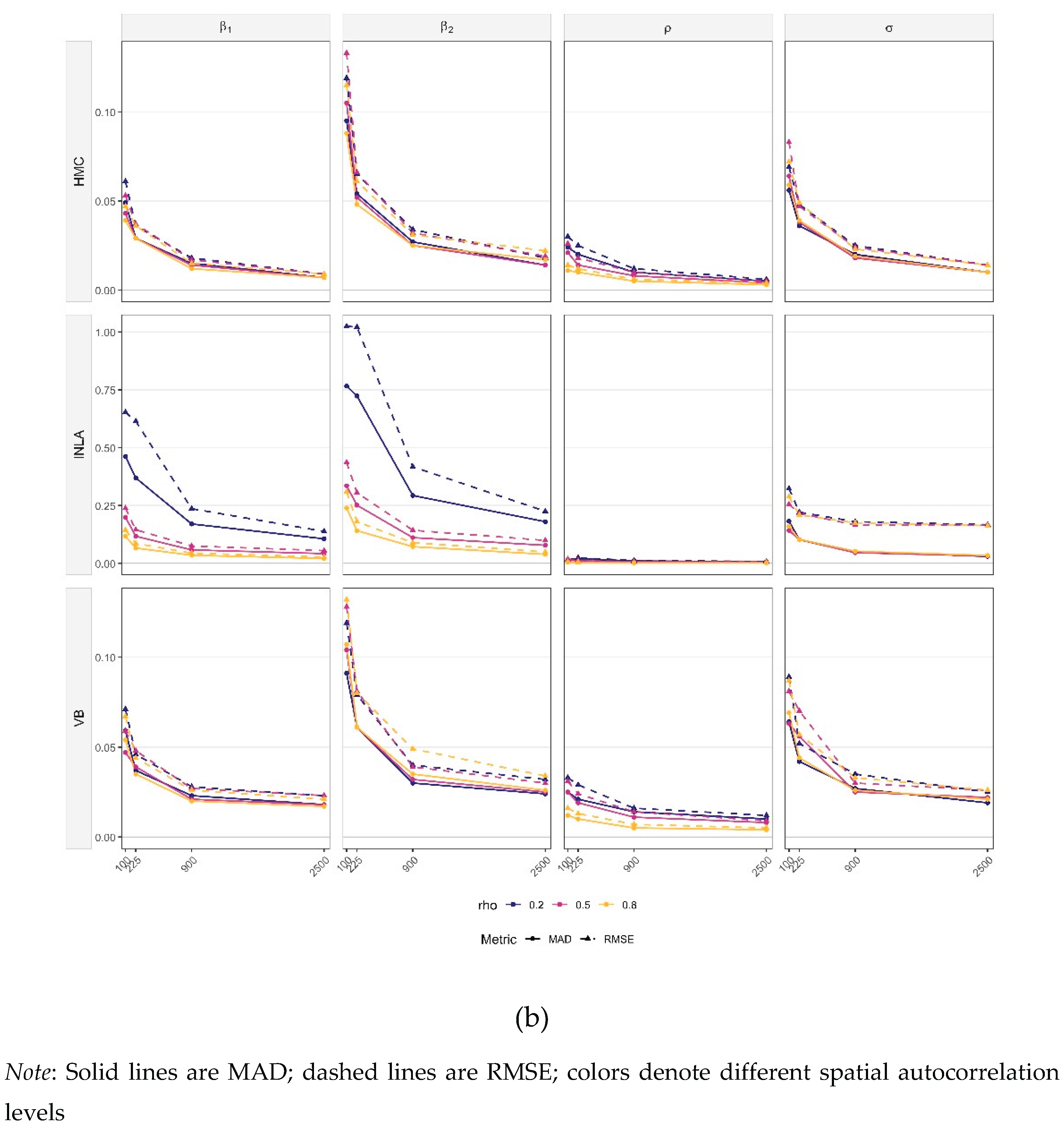
Figure 2.
(a) Posterior distributions by parameter for SEMs under varying sample sizes and spatial autocorrelation levels. (b) RMSE and MAD vs.
Figure 2.
(a) Posterior distributions by parameter for SEMs under varying sample sizes and spatial autocorrelation levels. (b) RMSE and MAD vs.
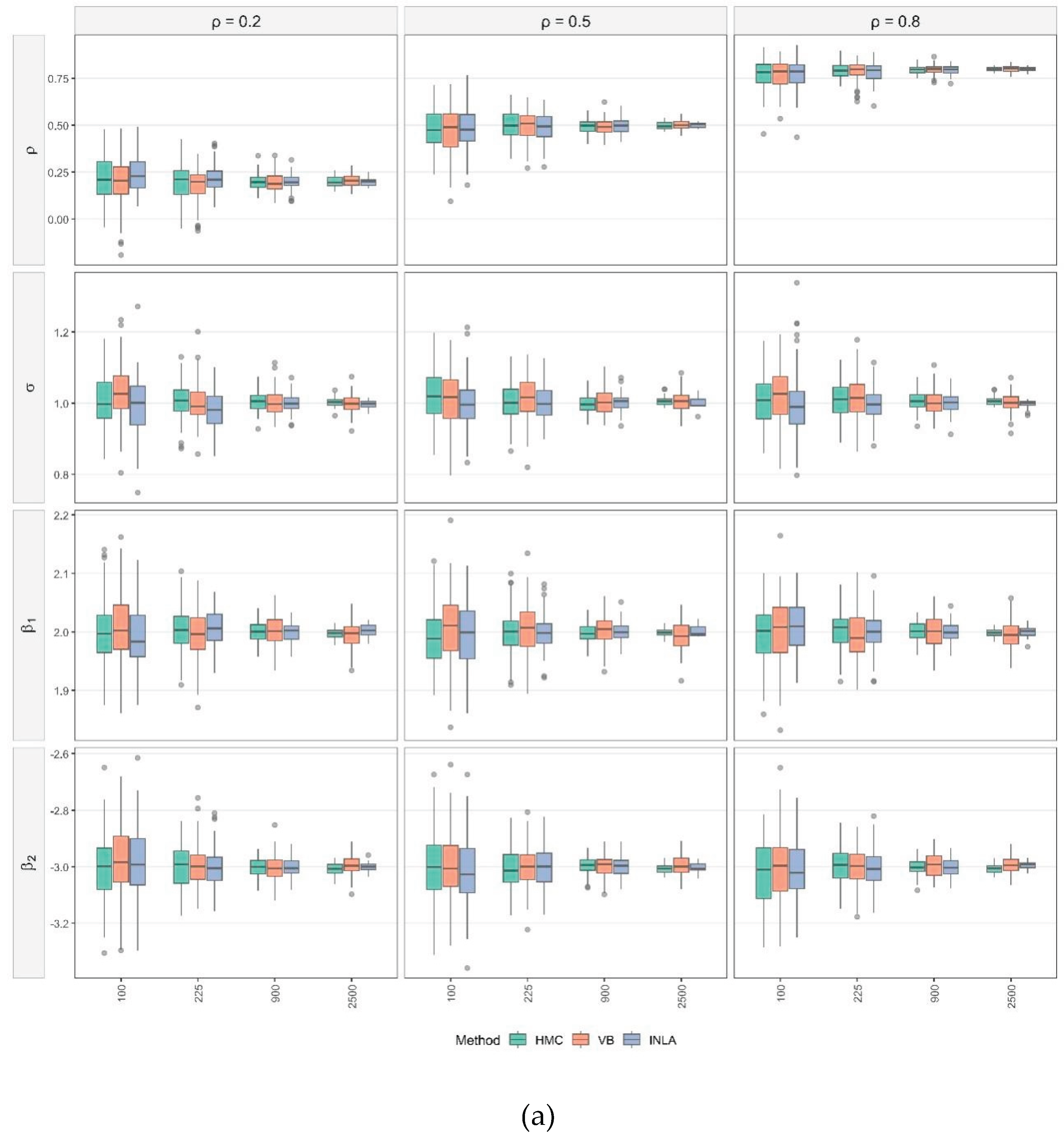
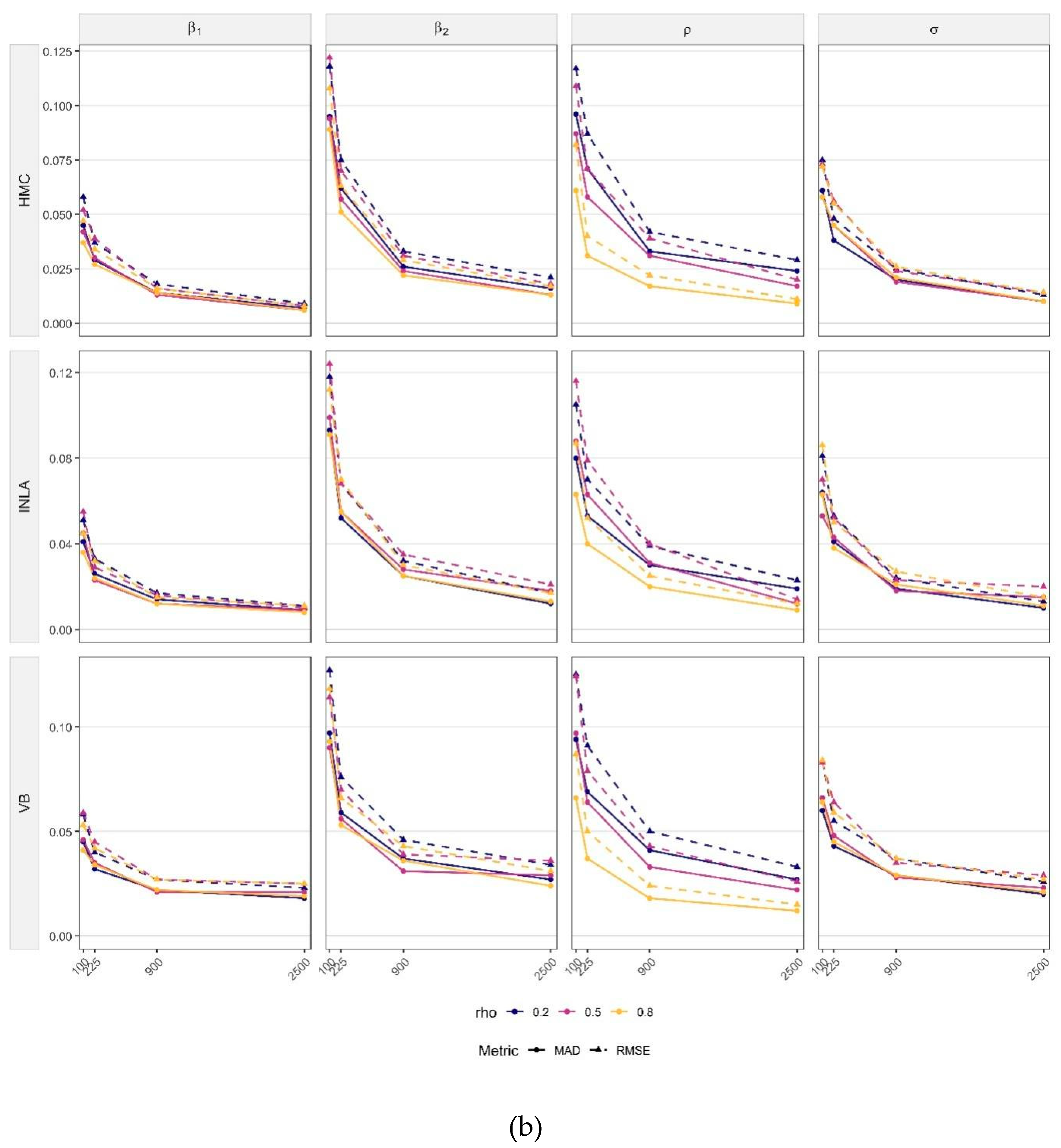
Figure 3.
Running time per simulation in seconds for two models using different Bayesian methods across various simulation scenarios.
Figure 3.
Running time per simulation in seconds for two models using different Bayesian methods across various simulation scenarios.
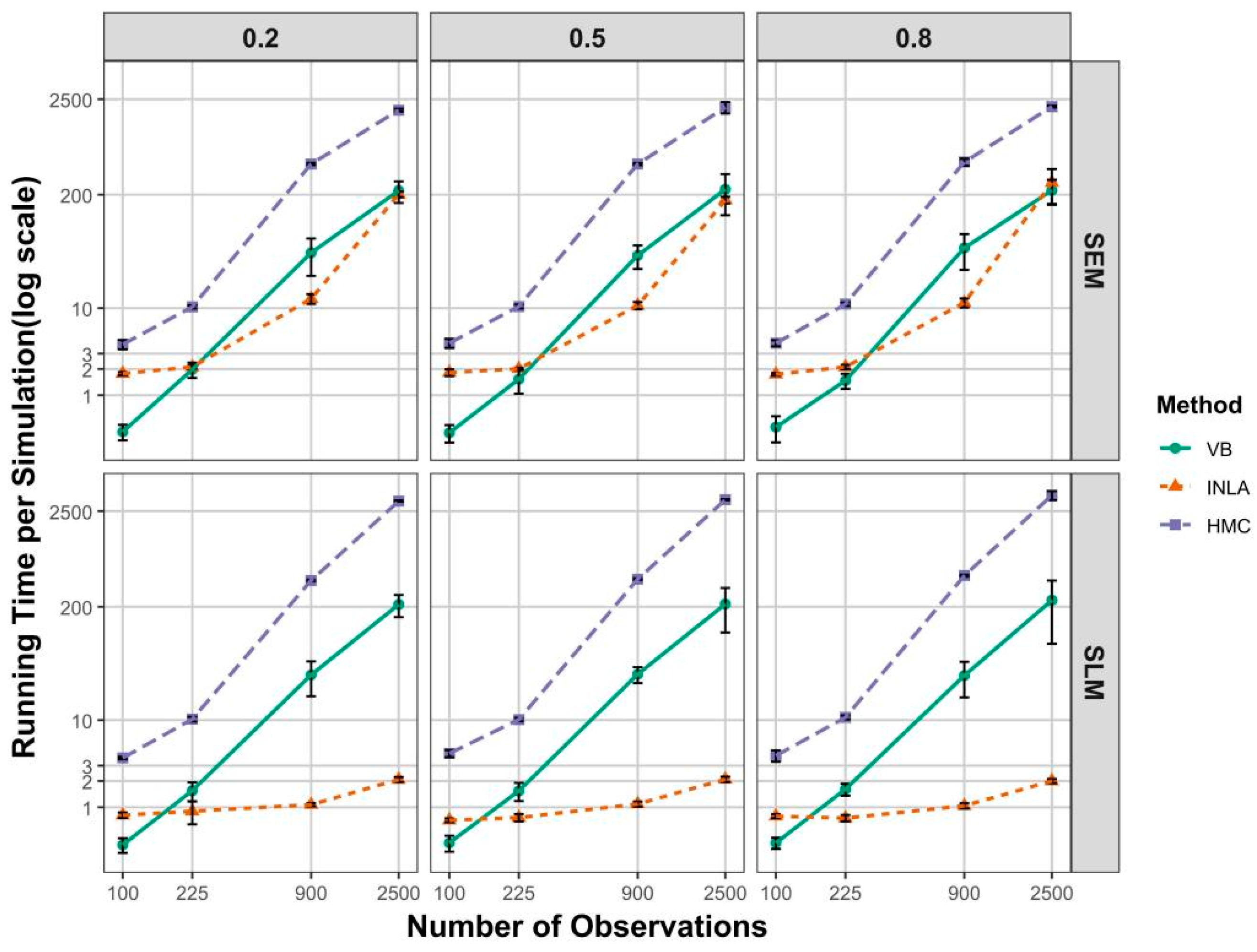
Figure 4.
Bayesian method selection matrix.
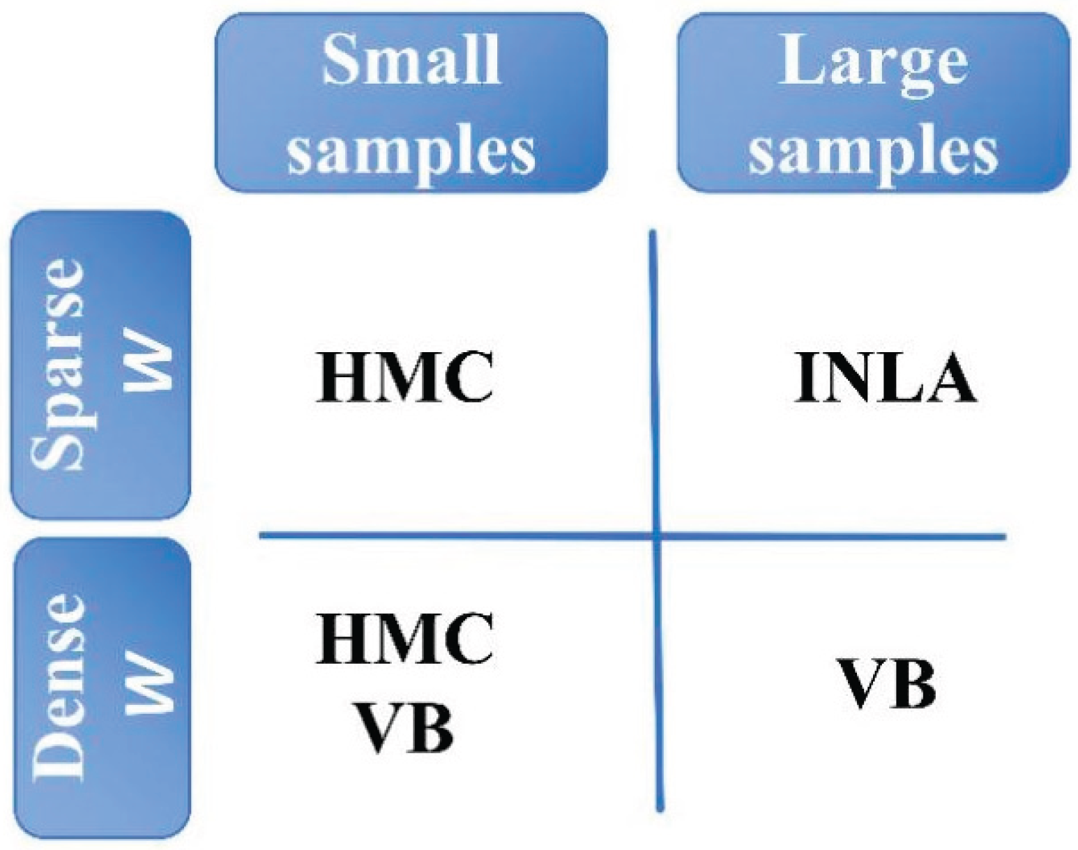
Table 1.
Simulation results: sensitivity to the choice of
| Model | Bayesian techniques |
Param- eters |
||||||||||||||||||||
| Mean | SD | RMSE | MAD | Mean | SD | RMSE | MAD | Mean | SD | RMSE | MAD | Mean | SD | RMSE | MAD | Mean | SD | RMSE | MAD | |||
| SEM | HMC | 0.484 | 0.055 | 0.056 | 0.045 | 0.474 | 0.074 | 0.077 | 0.06 | 0.459 | 0.117 | 0.13 | 0.096 | 0.452 | 0.185 | 0.15 | 0.115 | 0.461 | 0.228 | 0.147 | 0.119 | |
| 1.005 | 0.024 | 0.025 | 0.02 | 1.005 | 0.024 | 0.025 | 0.02 | 1.004 | 0.024 | 0.025 | 0.02 | 1.005 | 0.024 | 0.022 | 0.018 | 1.005 | 0.024 | 0.022 | 0.018 | |||
| 2.001 | 0.017 | 0.018 | 0.014 | 2.001 | 0.017 | 0.018 | 0.014 | 2 | 0.017 | 0.018 | 0.015 | 2 | 0.017 | 0.015 | 0.012 | 2 | 0.017 | 0.015 | 0.012 | |||
| -3.002 | 0.032 | 0.033 | 0.026 | -3.002 | 0.032 | 0.033 | 0.026 | -3.002 | 0.032 | 0.034 | 0.027 | -3.003 | 0.032 | 0.033 | 0.026 | -3.003 | 0.032 | 0.033 | 0.026 | |||
| VB | 0.495 | 0.055 | 0.056 | 0.044 | 0.479 | 0.057 | 0.057 | 0.041 | 0.476 | 0.112 | 0.123 | 0.096 | 0.475 | 0.165 | 0.151 | 0.122 | 0.523 | 0.184 | 0.162 | 0.134 | ||
| 1.01 | 0.025 | 0.035 | 0.025 | 1.006 | 0.025 | 0.038 | 0.029 | 1.01 | 0.024 | 0.04 | 0.031 | 1.007 | 0.025 | 0.037 | 0.027 | 0.999 | 0.025 | 0.032 | 0.026 | |||
| 2 | 0.018 | 0.028 | 0.022 | 2 | 0.018 | 0.033 | 0.026 | 1.999 | 0.018 | 0.033 | 0.027 | 1.996 | 0.019 | 0.033 | 0.026 | 2.003 | 0.018 | 0.029 | 0.023 | |||
| -3.001 | 0.034 | 0.042 | 0.034 | -3.009 | 0.034 | 0.044 | 0.035 | -3.001 | 0.034 | 0.045 | 0.037 | -2.999 | 0.035 | 0.045 | 0.036 | -3.003 | 0.035 | 0.04 | 0.032 | |||
| INLA | 0.506 | 0.051 | 0.047 | 0.035 | 0.501 | 0.069 | 0.064 | 0.052 | 0.464 | 0.105 | 0.11 | 0.083 | 0.462 | 0.156 | 0.133 | 0.104 | 0.485 | 0.186 | 0.146 | 0.122 | ||
| 0.998 | 0.024 | 0.023 | 0.019 | 0.998 | 0.024 | 0.024 | 0.018 | 0.999 | 0.024 | 0.023 | 0.019 | 0.998 | 0.024 | 0.02 | 0.016 | 0.998 | 0.024 | 0.025 | 0.021 | |||
| 2.003 | 0.017 | 0.017 | 0.013 | 1.998 | 0.017 | 0.015 | 0.012 | 2.001 | 0.017 | 0.017 | 0.014 | 2.001 | 0.017 | 0.017 | 0.014 | 1.999 | 0.017 | 0.017 | 0.013 | |||
| -2.992 | 0.032 | 0.036 | 0.028 | -2.997 | 0.032 | 0.032 | 0.026 | -3.007 | 0.032 | 0.031 | 0.024 | -3.004 | 0.032 | 0.036 | 0.027 | -3.006 | 0.032 | 0.03 | 0.024 | |||
| SLM | HMC | 0.498 | 0.013 | 0.014 | 0.011 | 0.496 | 0.018 | 0.018 | 0.014 | 0.494 | 0.029 | 0.031 | 0.025 | 0.488 | 0.053 | 0.052 | 0.04 | 0.476 | 0.078 | 0.08 | 0.06 | |
| 1.002 | 0.024 | 0.022 | 0.018 | 1.005 | 0.024 | 0.025 | 0.02 | 1.004 | 0.024 | 0.025 | 0.02 | 1.005 | 0.024 | 0.022 | 0.018 | 1.005 | 0.024 | 0.023 | 0.018 | |||
| 2.001 | 0.018 | 0.018 | 0.015 | 2.001 | 0.017 | 0.018 | 0.015 | 2 | 0.017 | 0.018 | 0.014 | 2.001 | 0.017 | 0.015 | 0.013 | 2.001 | 0.017 | 0.016 | 0.012 | |||
| -3.002 | 0.032 | 0.032 | 0.026 | -3.002 | 0.033 | 0.033 | 0.027 | -3.002 | 0.033 | 0.034 | 0.027 | -3.003 | 0.032 | 0.034 | 0.026 | -3.003 | 0.033 | 0.033 | 0.028 | |||
| VB | 0.499 | 0.011 | 0.014 | 0.011 | 0.497 | 0.011 | 0.014 | 0.011 | 0.5 | 0.016 | 0.031 | 0.024 | 0.495 | 0.017 | 0.05 | 0.038 | 0.481 | 0.018 | 0.084 | 0.062 | ||
| 1.007 | 0.025 | 0.038 | 0.029 | 1.005 | 0.025 | 0.038 | 0.03 | 1.003 | 0.025 | 0.034 | 0.029 | 1.002 | 0.025 | 0.035 | 0.028 | 1.008 | 0.025 | 0.037 | 0.028 | |||
| 2.004 | 0.018 | 0.034 | 0.027 | 2 | 0.018 | 0.027 | 0.022 | 2 | 0.018 | 0.03 | 0.024 | 2.003 | 0.019 | 0.032 | 0.025 | 2.007 | 0.019 | 0.03 | 0.024 | |||
| -3 | 0.034 | 0.046 | 0.037 | -3.011 | 0.033 | 0.047 | 0.036 | -3 | 0.035 | 0.046 | 0.037 | -3.006 | 0.034 | 0.043 | 0.035 | -3.001 | 0.035 | 0.047 | 0.038 | |||
| INLA | 0.507 | 0.04 | 0.038 | 0.029 | 0.493 | 0.057 | 0.056 | 0.044 | 0.487 | 0.087 | 0.104 | 0.073 | 0.497 | 0.131 | 0.109 | 0.106 | 0.491 | 0.16 | 0.108 | 0.123 | ||
| 1.164 | 0.065 | 0.177 | 0.054 | 1.169 | 0.065 | 0.18 | 0.051 | 1.164 | 0.064 | 0.175 | 0.052 | 1.173 | 0.064 | 0.185 | 0.053 | 1.162 | 0.064 | 0.175 | 0.051 | |||
| 2.002 | 0.254 | 0.264 | 0.201 | 2.115 | 0.403 | 0.416 | 0.322 | 2.121 | 0.865 | 1.101 | 0.727 | 2.15 | 1.015 | 1.081 | 0.731 | 2.13 | 1.43 | 1.016 | 0.757 | |||
| -2.985 | 0.404 | 0.382 | 0.292 | -3.171 | 0.648 | 0.627 | 0.468 | -3.313 | 1.381 | 1.063 | 0.823 | -3.548 | 1.945 | 1.084 | 0.739 | -3.685 | 1.85 | 1.091 | 0.839 | |||
Table 2.
Comparative summary of Bayesian estimation methods.
| Method | Strengths | Limitations |
| HMC | High accuracy; flexible | Slow for large datasets; |
| VB | Very fast; scalable | Small-sample bias in |
| INLA | Excellent scalability; accurate in large samples | Sensitive to matrix sparseness; biased and in small samples |
Table 4.
INLA estimation of the SEM for housing prices in Ames.
| Variable | Current expenditure | |
| Mean | 95%CIs | |
| lnLot_Area | 0.067 | (0.047; 0.087) |
| lnTotal_Bsmt_SF | 0.048 | (0.042; 0.054) |
| lnGr_Liv_Area | 0.462 | (0.432; 0.491) |
| Garage_Cars | 0.088 | (0.076; 0.101) |
| Fireplaces | 0.059 | (0.046; 0.071) |
| Spatial error () | 0.683 | (0.654; 0.711) |
| Sigma () | 0.178 | (0.173; 0.183) |
| Computing time (s) | 268 | |
Disclaimer/Publisher’s Note: The statements, opinions and data contained in all publications are solely those of the individual author(s) and contributor(s) and not of MDPI and/or the editor(s). MDPI and/or the editor(s) disclaim responsibility for any injury to people or property resulting from any ideas, methods, instructions or products referred to in the content. |
© 2025 by the authors. Licensee MDPI, Basel, Switzerland. This article is an open access article distributed under the terms and conditions of the Creative Commons Attribution (CC BY) license (http://creativecommons.org/licenses/by/4.0/).
Copyright: This open access article is published under a Creative Commons CC BY 4.0 license, which permit the free download, distribution, and reuse, provided that the author and preprint are cited in any reuse.


