Specifications Table
| Subject area |
Environmental Science |
| More specific subject area |
Population density and distribution modelling/estimation |
| Name of your method |
Bayesian Hierarchical Small Area Population modelling, which integrated multiple data sources and spatial autocorrelation within the Integrated Nested Laplace Approximations and Stochastic Partial Differential Equations (INLA-SPDE). |
| Name and reference of original method |
- 1)
Bottom-up Population modelling: Wardrop N.A., Jochem W.C., Bird T.J., Chamberlain H.R., Clarke D., Kerr D., Bengtsson L., Juran S., Seaman V., Tatem A.J. (2018). “Spatially disaggregated population estimates in the absence of national population and housing census data.” Proceedings of the National Academy of Sciences 115, 3529–3537. https://www.pnas.org/doi/10.1073/pnas.1715305115
- 2)
INLA: Rue, Havard, Sara Martino, and Nicolas Chopin. (2009). “Approximate Bayesian Inference for Latent Gaussian Models by Using Integrated Nested Laplace Approximations.” Journal of the Royal Statistical Society, Series B 71 (2): 319–92 - 3)
SPDE: Lindgren, F., Rue, H., & Lindström, J. (2011). An explicit link between Gaussian fields and Gaussian Markov random fields: The stochastic partial differential equation approach. Journal of the Royal Statistical Society: Series B (Statistical Methodology), 73(4), 423–498 |
| Resource availability |
All the R codes and datasets used in this study including the simulation study and methods validation/application data are found in this GitHub repository. |
Background
Small area population count data support decision-making across all areas of governance. Estimating population numbers affected by disasters, delivering health interventions, planning for elections and allocating resources equitably all require reliable estimates of population distributions at small area scales (UNFPA 2020). Such data are typically collected through a national population and housing census, but these can become quickly outdated in settings with substantial population movements and spatially heterogeneous patterns of fertility and mortality that are hard to predict (Tatem 2022). In addition, in some areas of certain countries, it is sometimes not possible to directly collect such population data due to poor access, conflicts or other security challenges. To fill these data gaps, geospatial methods have recently been developed that leverage advances in satellite imagery, computer vision, geospatial computation and spatial statistics to produce small area population estimates across national extents (e.g., Leasure et al., 2020; Boo et al., 2022; Darin et al, 2022; Nnanatu et al., 2024).
‘Bottom-up’ population models leverage the statistical relationships between population density measures in incomplete enumerations of an area of interest and a set of geospatial datasets capturing features known to correlate with how humans distribute themselves on the landscape. Predictions of numbers of residents for 100 by 100m grid cells are then typically made, and the use of Bayesian statistical inference methods for the estimation of the population model parameters means that estimates of uncertainties can be provided (Wardrop et al., 2018). However, the input enumeration data which can come from purposely designed ‘microcensus’ surveys (e.g. Leasure et al, 2020; Boo et al., 2022), incomplete census enumeration (e.g. Darin et al, 2022), or listings from household surveys (e.g. Dooley et al, 2021), are typically sparsely distributed and often exhibit spatial autocorrelation (Chan-Golston et al., 2022). In such situations, the integration of spatial autocorrelation within the analytical framework is highly recommended (Anselin, 1990; Chi & Voss, 2011; Chan-Golston et al., 2022).
Existing bottom-up population models (e.g., Leasure et al., 2020; Boo et al., 2022; Darin et al, 2022), use Bayesian hierarchical regression models to more accurately represent levels of variabilities within a single source of observed enumeration data as random effects, and quantify uncertainties in the parameter estimates in a more straightforward manner. Here, with an aim of improved accuracy in small area population predictions, we extend the existing approach to allow for the integration of multiple disparate enumeration data sources to increase sample size and obtain larger statistical power. We do this while simultaneously accounting for spatial autocorrelation within the observations to borrow strength (e.g., Chi & Voss, 2011) from nearby locations and more accurately predict population counts in non-sampled locations.
Motivated by the need to rapidly produce small area population data for Cameroon using multiple household listing datasets, we used geostatistical modelling frameworks (Cressie, 1993; Wakefield, 2007; Diggle & Giorgi, 2016; Giorgi et al., 2018), to imply spatial autocorrelation as a distance dependent covariance matrix, such that population distribution between nearby locations is more similar than those further apart (Tobler, 1970). To increase computational efficiency, the integrated nested Laplace approximation (INLA; Rue & Held, 2005; Rue et al., 2009) was used in conjunction with the stochastic partial differential equation (SPDE; Lindgren et al., 2011).
Method Details
Method
Within the context of the bottom-up population modelling (Wardrop et al., 2018), we are often faced with the problem of population prediction at high resolution regular grid cells (pixels) in order to build a set of estimates that can be flexibly summarised and aggregated to other decision making using, for example, administrative units, health zones, wards, or facility catchment areas, including areas where little or no data are observed. In most cases, population enumeration data are only available at some locations, for example, census units (CUs), primary sampling units (PSUs) or enumeration areas (EAs), across a given geographical domain of interest.
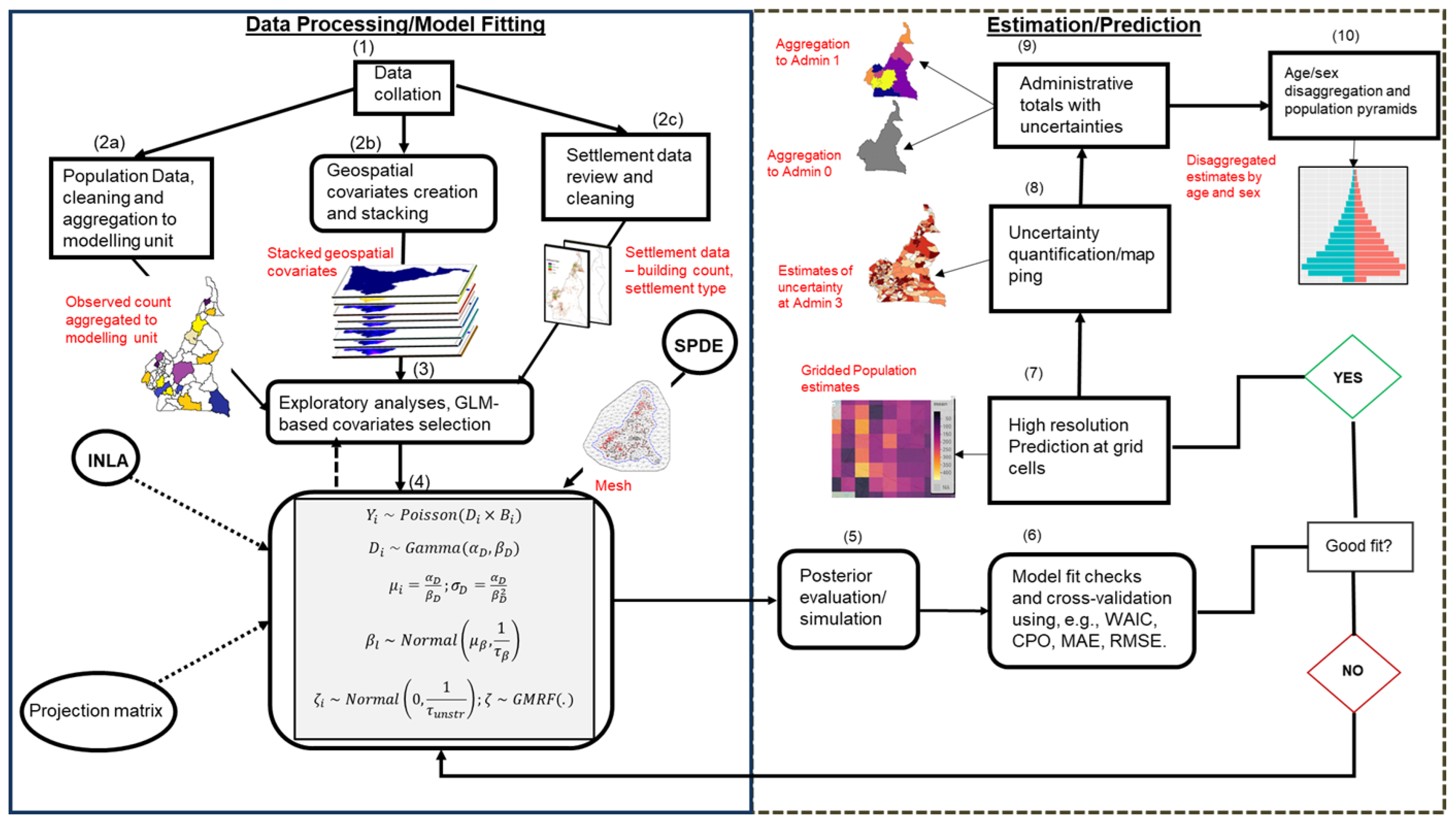
Figure 1 shows the schematic representation of the entire population modelling process developed here to address this problem. Specifically, in step 1, the input datasets were first assembled from the disparate sources. These datasets include the enumeration data (containing population counts of people within geographically defined small areas), the gridded geospatial covariates, (e.g., night-time lights intensity, road density, topography, land cover, distance to markets (Nieves et al., 2017)), and the settlement data (e.g. gridded data summarising buildings mapped from satellite imagery (Chamberlain et al., 2024), containing counts of building, building height estimates and other derived metrics). In step 2, these datasets were explored, cleaned, and prepared for the next steps. Part of the exploratory data analysis was testing for the presence of spatial autocorrelation in the observed data using Moran’s I statistics (Moran 1950) under the null hypothesis of no spatial clustering. Then, a statistically significant test indicates the presence of spatial autocorrelation.
To ensure that spurious effects of redundant geospatial covariates are eliminated in the model parameter estimates, a rigorous covariate selection process is carried out in step 3, where only the covariates that significantly predicted population density are retained for the final analysis. Fior a given location , the population density variable was obtained as the number of people () per building (), that is, = . The continuous geospatial covariates are scaled using z-score so that the parameter estimates based on the datasets emanating from disparate measurement scales can be compared and interpreted in terms of standard deviation. The covariates selection is done using a robust stepwise regression scheme implemented within the Generalized Linear Model (GLM) framework (McCullagh & Nelder, 1989) with the stepAIC function of the ‘MASS’ package in R. Then the selected covariates were further tested to ensure that the potential effects of multicollinearity are drastically reduced. To do this, we used the ‘vif’ function of the ‘car’ package in R to calculate the variance inflation factor (vif) values of each covariate and those with vif < 5 are retained (e.g., James et al.,2013). Finally, the GLM model was refitted and only the statistically significant covariates were retained for the next steps.
In step 4, the geospatial covariates selected in step 3 were used to train Bayesian hierarchical population models using the INLA-SPDE approach. The INLA-SPDE approach provides computational efficiency by using a mesh which is a triangulation of the entire spatial domain of interest allowing the use of sparse covariance matrix on a discrete space instead of a dense covariance on a continuous space (Lindgren et al., 2011).
Steps 5 to 10 follow immediately after model fitting and involved the collation and testing of the model results, posterior predictions at high resolution (approximately 100m by 100m) grid cells, aggregation to various administrative units of interest, and disaggregation of the population totals by age/sex classes.
The model fit assessments and cross-validation of the statistical models were performed by comparing a constellation of model fit metrics. Specifically, for model selection, we relied on the Deviance Information Criterion (DIC), the Widely Applicable Information Criterion (WAIC; Watanabe, 2013) and Conditional Predictive Ordinate (CPO; Pettit 1990). The predictive ability of the selected models were further evaluated using Mean Absolute Error (MAE), Root Mean Square Error (RMSE), Absolute Bias (BIAS), and the Pearson correlation coefficients (CORR) of the observed versus predicted population counts. Smaller values of the DIC, WAIC, and CPO indicate a better fit model. Also, smaller values of MAE, RMSE, BIAS, and larger values of CORR indicate model with better predictive ability. Posterior simulations and grid cell predictions were based on the best-fit model. Finally, by dividing the observed data into train (80%) and test (20%) sets, k-fold cross-validation was carried out.
Statistical Modelling
Let
denote the response variable, the count (population) of people in each small area
(
), such that
with equal mean and variance equal to
(McCullagh and Nelder 1989). However, it is well known that within the context of population modelling, the data are almost always over-dispersed in that the variance of the response is often larger than the mean and the assumption of equal mean and variance is rarely met (Leasure et al., 2020; Boo et al., 2022).
To circumvent this analytical challenge and improve estimates of population whilst accounting for potential sources of variability, the response variables is redefined in terms of population density (e.g., Leasure et al. 2020) so that
where the term
is generic and represents any variable that provides an indication of human settlement intensity within a given area, such as, the total built-up area, number of buildings, number of households, and building intensity, all typically obtained from satellite imagery feature extraction. However, the values of any such settlement variable must be available throughout the country for country-wide model prediction purposes. Thus, the term
represents the population density,
. For ease of exposition, from now on, we will use building count (number of buildings in each area of interest)
as the
variable and using a Poisson-Gamma two-stage model (e.g., Wakefield, 2007). Equation (1) becomes
where the mean and variance parameter
of Equation (1) is now respecified in terms of the expected density
and building counts
of area
, that is,
and
is the population density which gives the Maximum Likelihood Estimator (MLE) for
. Thus, the model specification in equation (3) allows us to model explicitly the potential overdispersion within the data via the mean density parameter by assuming a Gamma distribution with shape and rate parameters given by
and
, respectively. That is,
where
and
. Note that the choice of the Poisson-Gamma two-stage model is because it allows flexibility to explicitly model the inherent overdispersion via the parameter
. Other positively skewed long tail distribution such as the LogNormal distribution (e.g., Leasure et al, 2020) could also be used, so that,
, where
and
are the log of the expected population density and the random variations in the population density due to overdispersion, respectively.
Despite the simplicity of the specification implied by equation (3), it is important to note that the variance of
increases for very small values of
which could arise from sparse observations (e.g., Wakefield, 2007). Thus, to avoid inflated population estimates, care must be taken while using this model specification to account for either overdispersion or as aggregation weights to account for potential aggregation error (e.g., Paige et al. 2022). In any case, the expected population density
is linked to the geospatial covariates (e.g., nighttime lights, distance to healthcare facilities) through the linear predictor
given by
where
is an appropriate link function (e.g., log-link),
is the intercept parameter representing the average population density when there is zero effect of the other covariates;
are the unknown fixed effect coefficients of the K geospatial covariates
found to significantly predict the population density;
is a Gaussian noise or nugget effect (Cressie, 1993), which accounts for the observation level variability (also known as the fine scale variability, e.g., Paige et al., 2022) not captured by the geospatial covariates, that is,
. To ensure that the estimates of the fixed effects parameters
are interpretable and comparable, it is recommended that the corresponding continuous geospatial covariates which are potentially on different measurement scales be rescaled using for example the z-score such that
where
is the scaled version of the geospatial covariate
.
Specifically, we extended equation (5) to include the spatial autocorrelation term
such that the geographical units that share common boundaries are more like each other in terms of population distribution than those further apart (Tobler, 1970). Thus,
where
is the linear predictor,
is the
-th spatial unit (e.g., enumeration areas) of the
geolocated spatial units within the study domain. The term
is the
-th realisation of the Gaussian Random Field (GRF), that is,
, with the distance dependent Matérn covariance function
where
is a gamma function;
is the modified Bessel function of the second kind, order
;
is the Euclidean distance between spatial locations
and
;
is the smoothness parameter;
is the scale parameter where
is the spatial distance at which the correlation is approximately 0.13;
is the marginal variance. One computational challenge of geostatistical models of this form especially those implemented via the Markov chain Monte Carlo (MCMC) methods is that the computation of the dense covariance matrix
becomes very expensive as the sample size increases (e.g., Bakka et al., 2018). However, the use of the integrated nested Laplace approximation in conjunction with the stochastic partial differential equation (INLA-SPDE; Rue and Held, 2005; Rue et al., 2009; Lindgren et al., 2011) approach provide significant computational advantage. With the INLA-SPDE approach we only need to compute the sparse precision matrix
, and the continuously indexed GRF,
is approximated by a discretely indexed Gaussian Markov Random Field (GMRF) using a piecewise linear basis function representation on a triangulation of the entire study domain also known as ‘mesh’. Thus,
where
is the value of the piecewise linear function which takes the value of 1 at the
-th node of the mesh and 0 elsewhere for a mesh with a total of
nodes;
is a GMRF with sparse correlation matrix parameters
and
(see, Lindgren et al., 2011; Blangiardo et al., 2013). Thus, under the INLA-SPDE approach, equation (7) is respecified as:
where
is the
-th element of the
sparse projection matrix
which maps the
observations to the
nodes of the mesh. Note that it is straightforward to extend equation (10) to include other random effects terms to capture other unobserved sources of variability like those due to settlement type (rural-urban), regions, data source, interacting random effect terms, etc. Thus, the hierarchical regression-modelling framework is specified below:
where
are the random effect functions of the M different data sources; while
,
, and
capture the variabilities due to differences in population distributions across different settlement types, regions, and their interactions, respectively. As stated above, the framework allows the incorporation of as many random effects as possible, however, care must be taken to avoid overfitting the data.
Bayesian Inference for Hierarchical Population Models
In Bayesian inference context, interest is on the joint posterior distribution of the latent field
and the hyperparameters
given by
where
is the prior distribution,
is a latent Gaussian model (LGM), and
is the likelihood function of observing the data given the latent field and the hyperparameters which are assumed to be conditionally independent. The posterior distribution is then approximated and evaluated using INLA-SPDE as already stated above with prior distributions given by:
where
and
are hyperparameters and
. Then the predicted density
is obtained as the back transformed values of the predicted linear predictor
, that is,
Finally, the predicted population count is given as a weighted product of the population density and the building count, that is, .
Model Fit Checks and Cross-Validation Metrics
Conditional Predictive Ordinates (CPO)
The CPO is a cross-validatory criterion which calculates the probability of observing a held-out observation not used in the model training set such that given the
-th observation
. Thus, the CPO is the posterior probability of observing
when the model is fit using all data but
, that is,
Large values of CPO indicate a better fit of the model to the observation, while small values indicate a bad fitting of the model to that observation, which may be an outlier.
Then, the negative sum of the log of the CPO given in equation (14) provides a measure of predictive ability of the model with the smaller the better, that is,
Mean Absolute Error (MAE)
The mean absolute error (MAE) provides a measure of the average magnitude of errors within a set of predictions irrespective of the direction. It is calculated using
where,
and
are the observed and predicted values, respectively. The model with the smaller MAE value provides a better fit.
Root Mean Square Error (RMSE)
The root mean square error (RMSE) is similar to the MAE in that they both provide an idea on the average magnitude of prediction error. However, the RMSE is found to be more useful when large errors are not desirable. RMSE is given by
Similar to the MAE, models with lower RMSE values provide better fit.
Pearson Correlation
The Pearson correlation coefficient
) is the coefficient of correlation between the observed counts and predicted counts.
where
and
are the observed values, mean of the observed values, the predicted values, and the mean of the predicted values, respectively. Note that equation can be simply written as
where,
is the covariance between the observed
and the predicted value
, and
,
, are the corresponding standard deviations.
Absolute Bias (BIAS)
This measures the average deviation of the predicted value from the observed value:
Smaller values of BIAS indicate better fit model. The closer the value to zero the better the model.
Coefficient of Variation
For each posterior sample, we computed the coefficient of variation as a measure of uncertainty in the posterior parameter estimation. This was done by dividing the standard deviation with the.mean.
Motivating Dataset
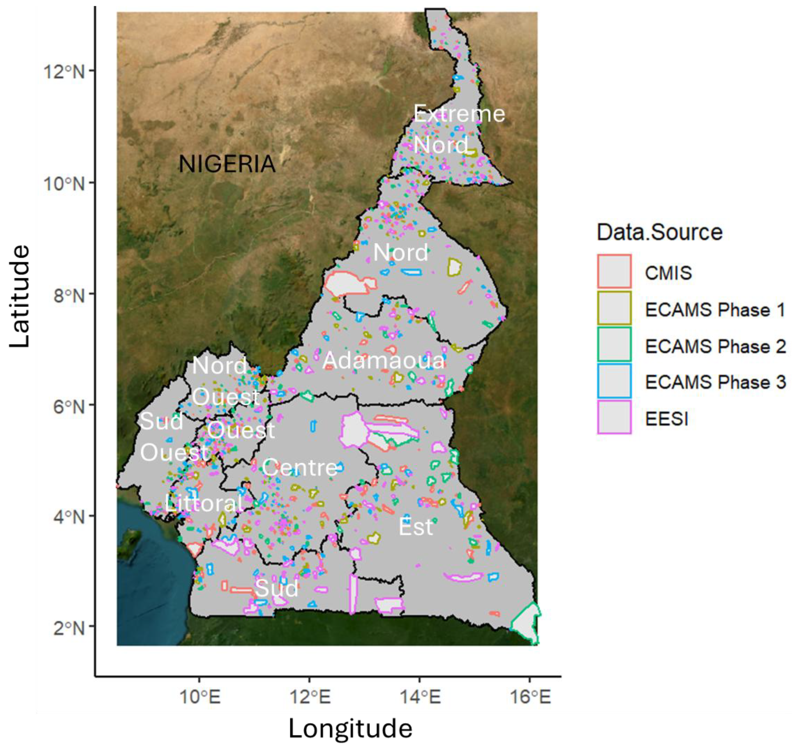
This study was motivated by the lack of a reliable up-to-date small area population data to support healthcare campaigns and other intervention programmes in Cameroon, and to build an alternative sample frame given that the most recent census at the time of writing was conducted in 2005. Completely anonymized versions of seven (7) nationally representative but disparate household listings conducted between 2018 and 2022, were obtained from the Cameroon National Institute of Statistics (NIS), also known in French as
Institut National de la Statistique (INS,
https://ins-cameroun.cm/en/). Following rigorous data cleaning and exploratory activities, five of these datasets conducted between 2021 and 2022 were selected for population modelling (
Figure 2). There were 2,587,569 people counted across the 509,628 households with an average of ~5 people per household, across 2,290 Enumeration Areas (EAs). Eventually, the datasets were combined and aggregated up to the EA level which served as the population modelling unit. Further details on how the datasets were explored, cleaned and combined are provided within Section S1 of the Supplementary document.
Testing for Spatial Clustering
Before proceeding to analyse the data, we first carried out Moran’s I test for the existence of spatial autocorrelation using the ‘moran.test’ function of the ‘spdep’ package in R, after defining the neighbourhood structure using the ‘queen’ option. However, the Moran’s I test statistic returned a statistically significant test with p-value < 0.01 which indicated the presence of spatial autocorrelation within the data.
Statistical Model Implementation
Following from equations (1) – (11) above, the observed data (the total number of people observed per EA) is Poisson distributed random variable with mean/variance parameters , where is the average population density per EA, and is the total number of buildings (total building counts) per EA. The building counts were obtained from the building footprint layer provided by the Digitize Africa project of Ecopia AI and Maxar Technologies (‘year 2’, 2020/2021; Ecopia.AI and Maxar Technologies, 2020). The building footprint layer contains polygons representing visible individual buildings on satellite images. This was rasterised using WorldPop’s 3-arc-sercond resolution mastergrid to calculate number of buildings, building area, building perimeter, coefficient of variation, and other related metrics for each grid cell.
Figure S1.1 of the Supplementary document shows the rasterised building footprints and the settlement type classifications of the structures in Cameroon. The settlement type classification was obtained from the Global Human Settlement (GHS) degree of urbanization layer (Schiavina, 2022), which was re-classified into four settlement types namely: cities, small urban, towns and villages.
Model Fitting
Of the 43 geospatial covariates initially identified (
Table S1 of the Supplementary document), after covariates selection using the GLM-based stepwise selection methods (McCullagh & Nelder, 1989; James et al., 2013), only 8 were eventually retained as providing the best fit for the population density model (
Table 1).
The 8 final geospatial covariates were then used to test various nested Bayesian hierarchical models, and the four top competing nested models are specified below:
where, the terms
,
,
,
, and
are intercept, fixed effect coefficients of the 8 geospatial covariates (
Table 1)
(
),
projection matrix, spatial autocorrelation term, settlement type (4 classes – cities, small urbans, towns and villages), settlement type – region interaction term, and the zero mean Gaussian nugget effect, respectively. The 10 regions in Cameroon along with the 4 settlement classes constituted a total of
settlement type versus region interaction effects.
Figure S3.1C of the supplementary material shows the mesh with 534 vertices which was employed for the model implementation. More details about the design of mesh can be found in Gomez-Rubio (2020) and some of the references therein. The projection matrix
maps the observations unto the mesh nodes to facilitate computational efficiency at the mesh nodes.
Prior Distribution
Initial sensitivity analyses which involved the testing of various priors and hyperprior values indicated that the following INLA default priors and hyperpriors provided no worse fit:
However, an alternative prior specification using a joint penalized complexity (PC) prior (Simpson et al. 2017) could still be used.
Finally, the predicted population density
is obtained by as the exponent of the linear predictor, that is,
So that the predicted population count is obtained deterministically as .
Model Fit Checks
When implemented to the Cameroon combined household listing data, model 4 (which included spatial autocorrelation, settlement type and settlement type - region interactions random effects) has the lowest DIC and lowest
according to
Table 2, thus, provided the best fit for the data. This underscores the importance of jointly accounting for spatial autocorrelation and the random effects of data hierarchy across settlement types within various regions/administrative units within a bottom-up population modelling framework.
Posterior sampling and GRID Cell Predictions
The INLA-SPDE approach utilized here allowed us to generate posterior marginal distributions of the best fit model (Model 4) which allowed us to draw more samples from the stationary distribution and carry out Bayesian statistical inference. This was implemented by using the ‘inla.posterior.sample’ function of the ‘INLA’ package. However, to use the ‘inla.posterior.sample’ function, it needs to be activated during the model fitting by setting config = TRUE within the control.compute argument of the inla() function. The posterior samples were then used to predict population densities/numbers at high resolution prediction pixels. Further details of the posterior simulation and grid cell prediction approach are provided in Section S2 of the Supplementary document.
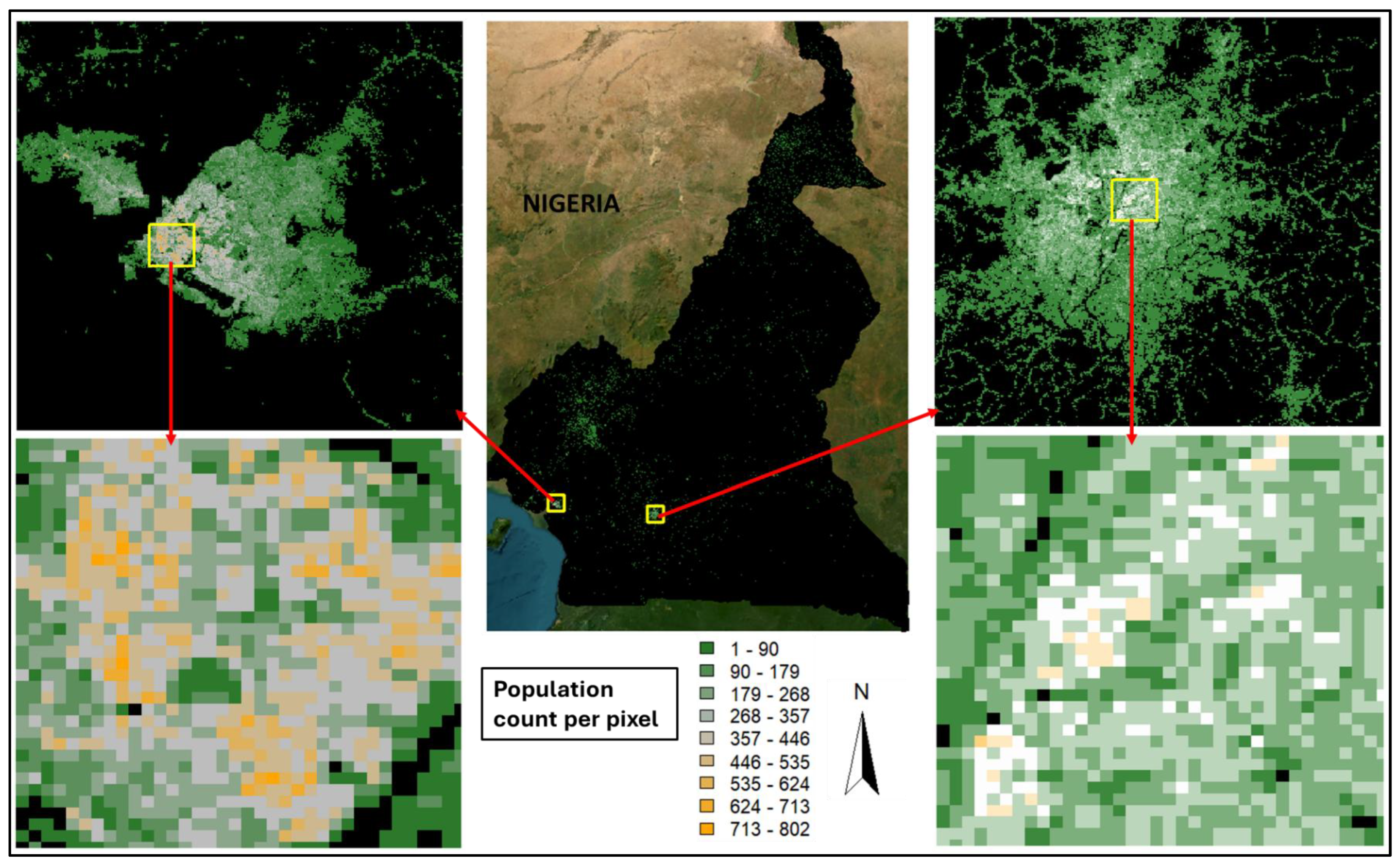
Posterior predictions of the mean population count per 100m square grid cell (or pixel) across the entire spatial domain along with the corresponding inset maps are provided in
Figure 3A. The inset maps focused on the two major cities in Cameroon, namely, Yaoundé which is the administrative capital located in the Central region of Cameroon, and Douala which is the commercial capital and located within the Littoral region of Cameroon (see
Figure 2). The zoomed in (inset) maps show overall higher population density and distribution per grid cell in Douala than in Yaoundé.
Figure 3A.
Predicted population counts across Cameroon at 100m-by-100m square, with corresponding inset maps created for the two major cities in Cameroon – Douala and Yaoundé. A minimum of ~1 and a maximum of ~799 people per grid cell was predicted across the country.This suggests the existence of more clustered but heterogeneous settlement patterns or higher concentration of various forms of residential high-rise buildings per grid cell in Douala than in Yaoundé. It could also mean that more high-rise buildings in Douala are used for residential purposes.
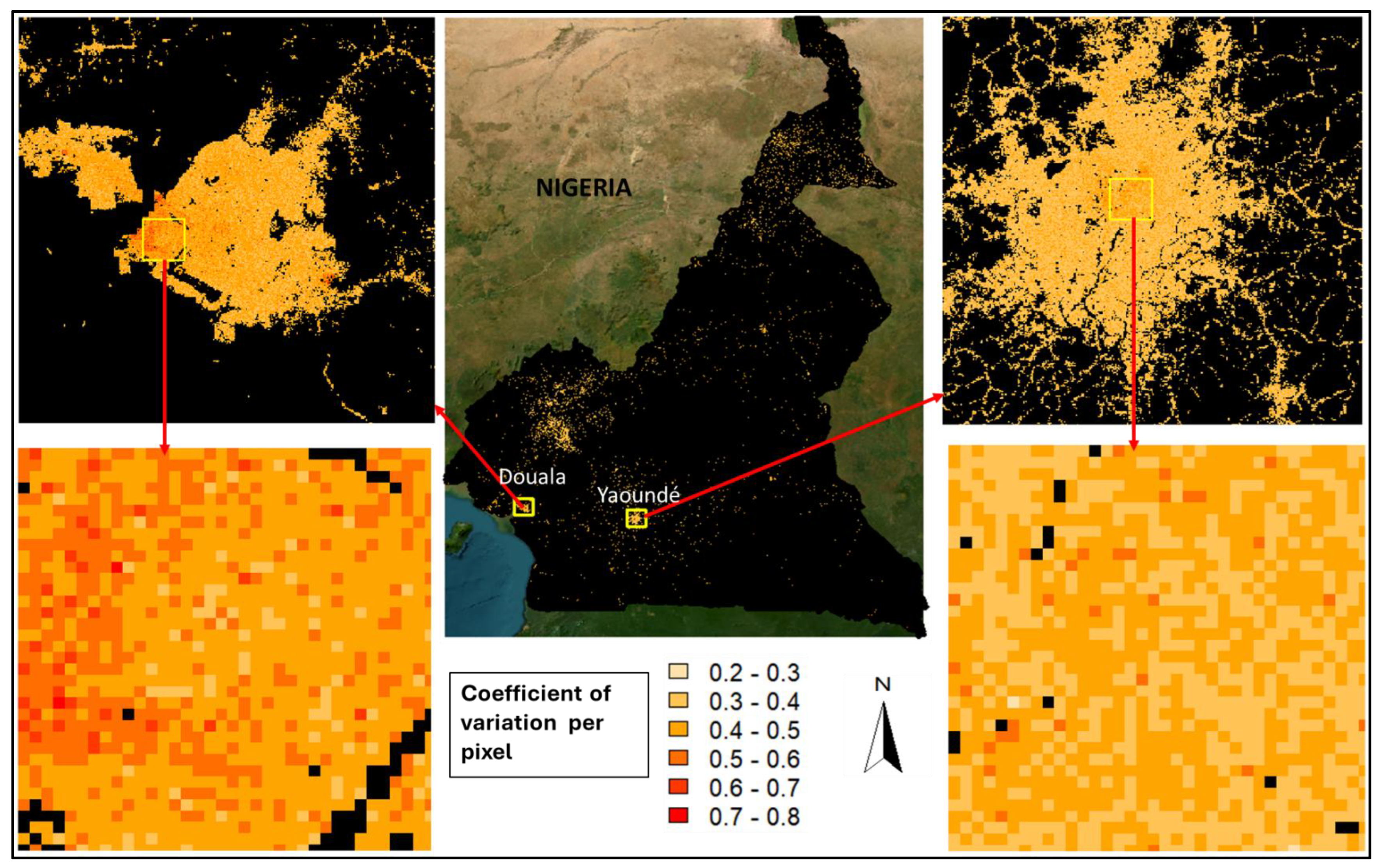
Figure 3B.
Coefficient of variation (CV) of the predicted mean of population counts across Cameroon at 100m-by-100m square, with corresponding inset maps created for and within the two major cities in Cameroon – Douala and Yaoundé.
Figure 3B.
Coefficient of variation (CV) of the predicted mean of population counts across Cameroon at 100m-by-100m square, with corresponding inset maps created for and within the two major cities in Cameroon – Douala and Yaoundé.
Estimates of uncertainties in the predictions of population counts across the grid cells were quantified through the coefficient of variations (CV) which was calculated as the ratio of the standard deviation of the predicted population count
and the predicted mean count
per grid cell. The CV provides the relative measures of variability across the grid cells and was provided across the entire spatial domain of Cameroon (
Figure 3B). The values of the CV ranged from 0.2 to 0.8 with the highest values obtained in the highest population density areas of Doula but in mostly lowest population density areas of Yaoundé (
Figure 3B, inset maps). The high variabilities in the high population density areas of Douala further reinforce the existence of more heterogeneous settlement patterns in Douala than in Yaoundé.
Method Validation
We used a two-pronged approach to validate our methods:
- 1)
A simulation study
- 2)
K-fold cross-validation using the combined real household listing datasets.
Simulation Study
First, the entire spatial domain was taken as a regular rectangle and divided into 11,008 grid cells at 10km-by-10km resolution (
Figure S3.1 of the Supplementary document). Note that the 10km square grid cell resolution was chosen for computational convenience while maintaining spatial detail, but any other resolution could be used. We used the Cameroon boundary file, which was provided by the Cameroon National Institute of Statistics (NIS) to crop the grid cells to align perfectly with Cameroon boundary (
Figure S2.1C). To check the impacts of spatial autocorrelation, first, we assumed that the entire population was completely observed, i.e. 100% survey coverage provided through five (5) different data sources. We simulated 3 datasets using different spatial variance parameter values set at
, where
- low spatial variance;
– moderate spatial variance; and
for high spatial variance. Other input parameter values used in the simulation are presented in
Table 3.
For each of the 3 initially simulated datasets, different levels of missingness or proportions of survey coverages were allowed – 100%, 80%, 60%, 40%, 20%. Thus, altogether, 15 datasets were simulated and tested. And for ease of exposition, variabilities across the different data sources were assumed to be similar with a variance parameter of 0.01. The R scripts used for the implementation of the simulation study are available on the GitHub repository here:
https://github.com/wpgp/Efficient-Population-Modelling-using-INLA-SPDE.
Model Fit Metrics (Simulation Study)
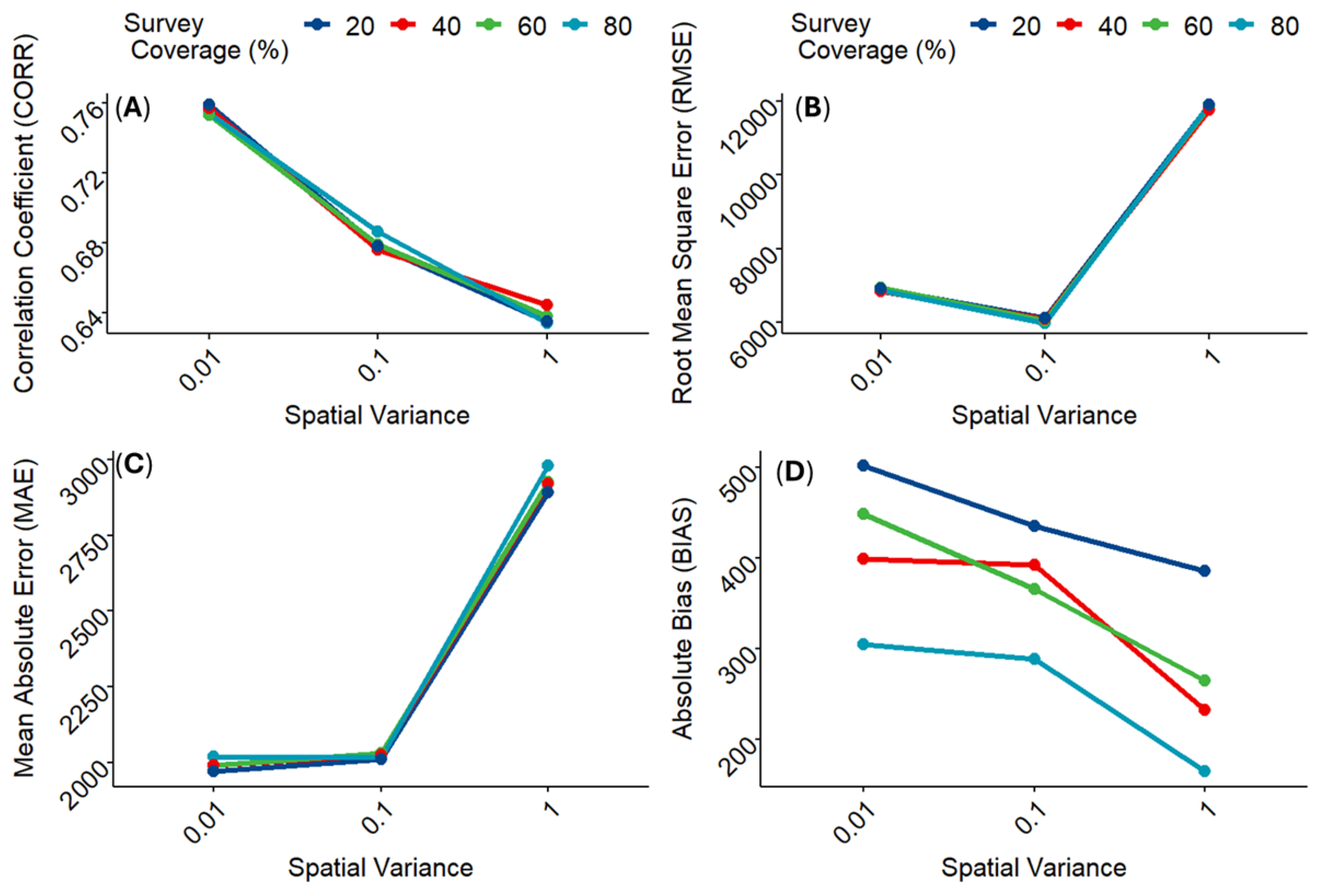
Figure 4 shows the model fit metrics calculated from the various combinations of the simulation parameter values. Apart from the absolute BIAS, model predictive ability increased with lower spatial variance across all fit metrics regardless of the proportion of missingness within the observed enumeration data. Interestingly, model predictive ability based on BIAS appears to be more sensitive to missingness proportions with model predictions becoming less accurate over lower spatial variance as the proportion of missing data increased. This finding underscores the importance of accounting for spatial variance/spatial autocorrelation while dealing with spatially clustered demographic datasets. But it also highlights the advantage of using multiple model fit metrics to validate and evaluate model performance.
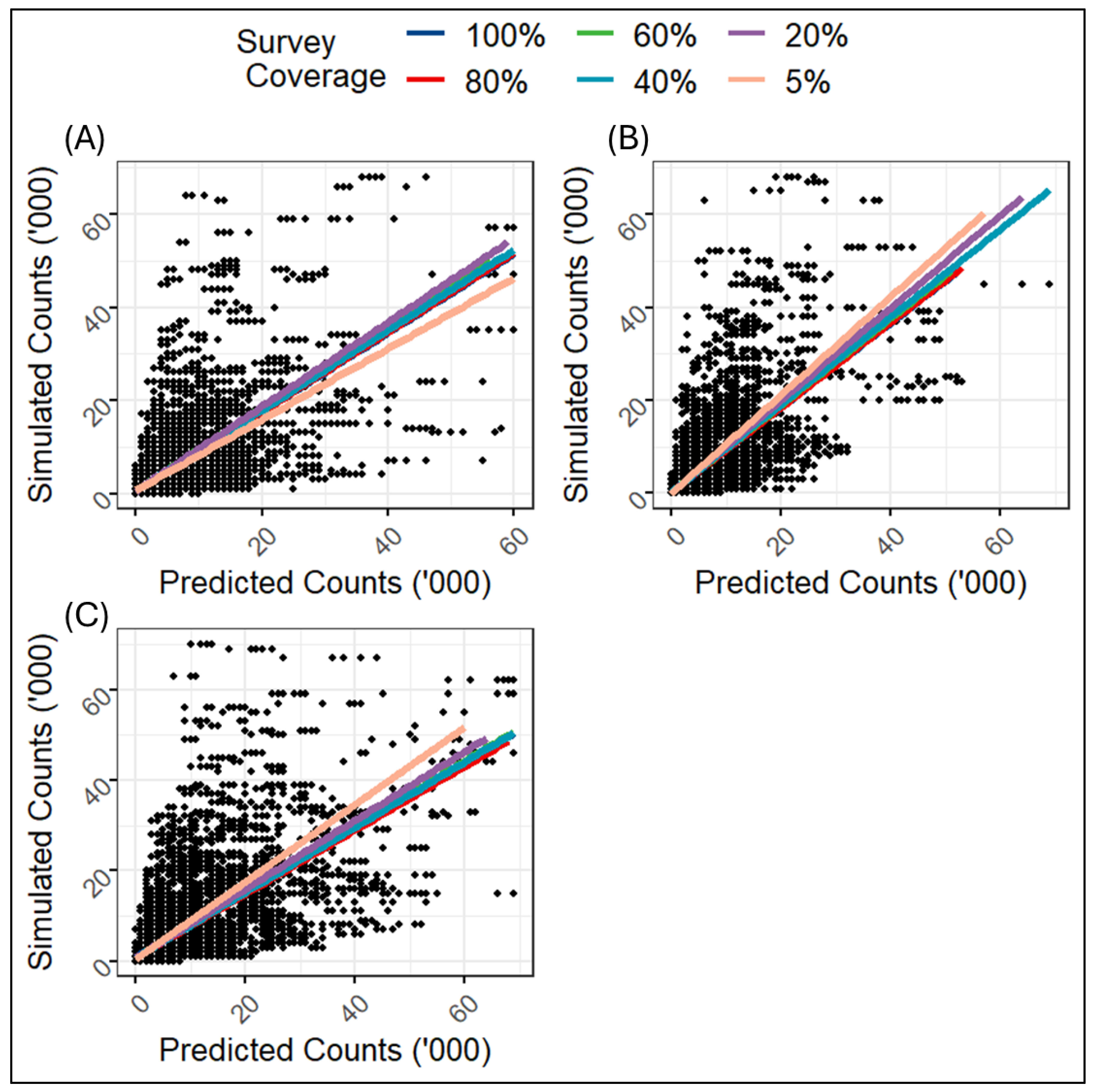
Further evaluation of the simulation study outputs was done by examining the correlations between the simulated population counts and the predicted population counts.
Figure 5 shows the scatter plots of the simulated counts versus predicted counts produced across the different levels of data missingness over different spatial autocorrelation structures (i.e., different levels of spatial variances). Overall, the predicted population counts across the various levels of survey coverage (or missingness) within each level of spatial variance, correlated nicely with the corresponding simulated population counts. However, there are indications of higher prediction accuracy of population count for higher spatial dependence (i.e., lower spatial variance). For example,
Figure 5B (moderate spatial variance) and
Figure 5C (high spatial variance) show evidence of overestimation of the population counts when compared to the low spatial variance scenario in
Figure 5A. This suggests a widening variability in the estimates of the population counts as the magnitude of spatial variance increased, thereby underscoring the importance of taking the potential effects of spatial autocorrelation into account in population modelling.
k-Fold Cross-Validation (Real Data Application)
k-fold cross validation was used to validate the proposed methodology and test the stability and the predictive ability of the model. Here, the observed motivating Cameroon dataset was used to investigate two forms of cross-validation approaches – in-sample and out-of-sample cross-validation. For the in-sample cross validation, all the datasets were used to train the model as described above. Then 20% of the data was randomly selected and used as a test set. In this case, the test set were random subsets of the training set. This was repeated for 5 times with a different set of test samples selected each time. For each fold, the values of the test samples were set to NA and then predicted using the model parameters. Model fit metrics were then computed and stored.
The out-of-sample cross-validation approach is slightly different and more rigorous. Here, the full data was randomly split into a 20% test set and 80% training set. The model was trained with the 80% training set, while the withheld values of the 20% test set were predicted using the trained model parameters. In this case, the test set was not part of the training set. As in the in-sample strategy, the k-folds test sets were non-overlapping, and the values of model fit metrics were calculated after model predictions with each test set. Thus, for each of the in-sample and out-of-sample cross-validations we used k {=5} folds. The model fit metrics calculated across all the folds for each method along with their average values are presented in
Table 3. Model fit metrics based on the two strategies were stable and similar, and there is an adequate average correlation coefficient of at least 98% for both strategies. The R scripts used for the implementation of the cross-validation strategies are available in the GitHub repository:
https://github.com/wpgp/Efficient-Population-Modelling-using-INLA-SPDE.
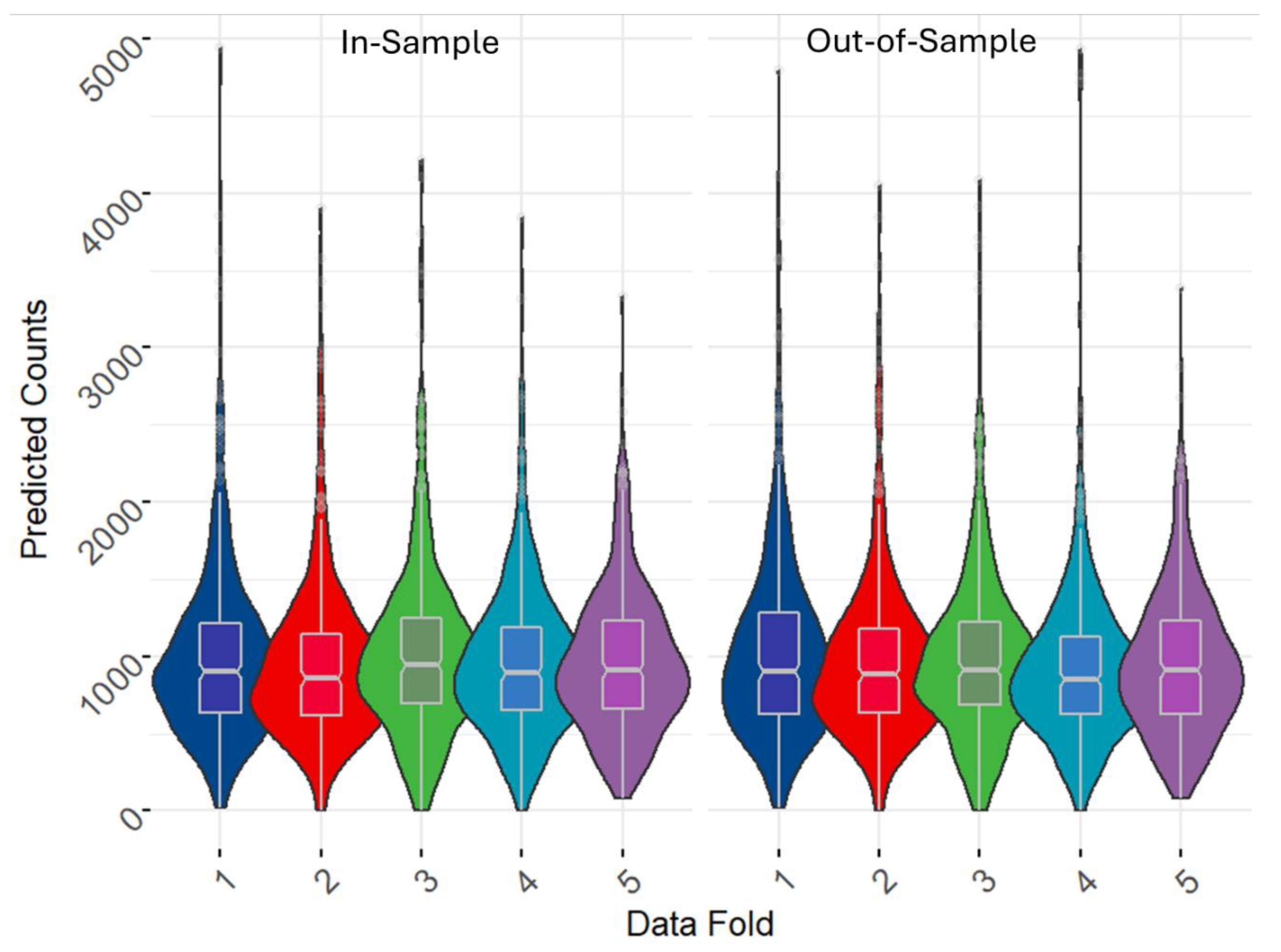
Additionally, we carried out a visual inspection of the cross-validation outputs by displaying the violin plots with embedded notched boxplots of the predicted population counts for each test set fold (
Figure 6). The findings further reinforced the outputs in
Table 4, which highlighted the high level of accuracy and efficiency of our methodology. There was good agreement between the predicted values across each corresponding folds for both the in-sample and out-of-sample strategies.
Comparing the Modelled Estimates with Projected Estimates
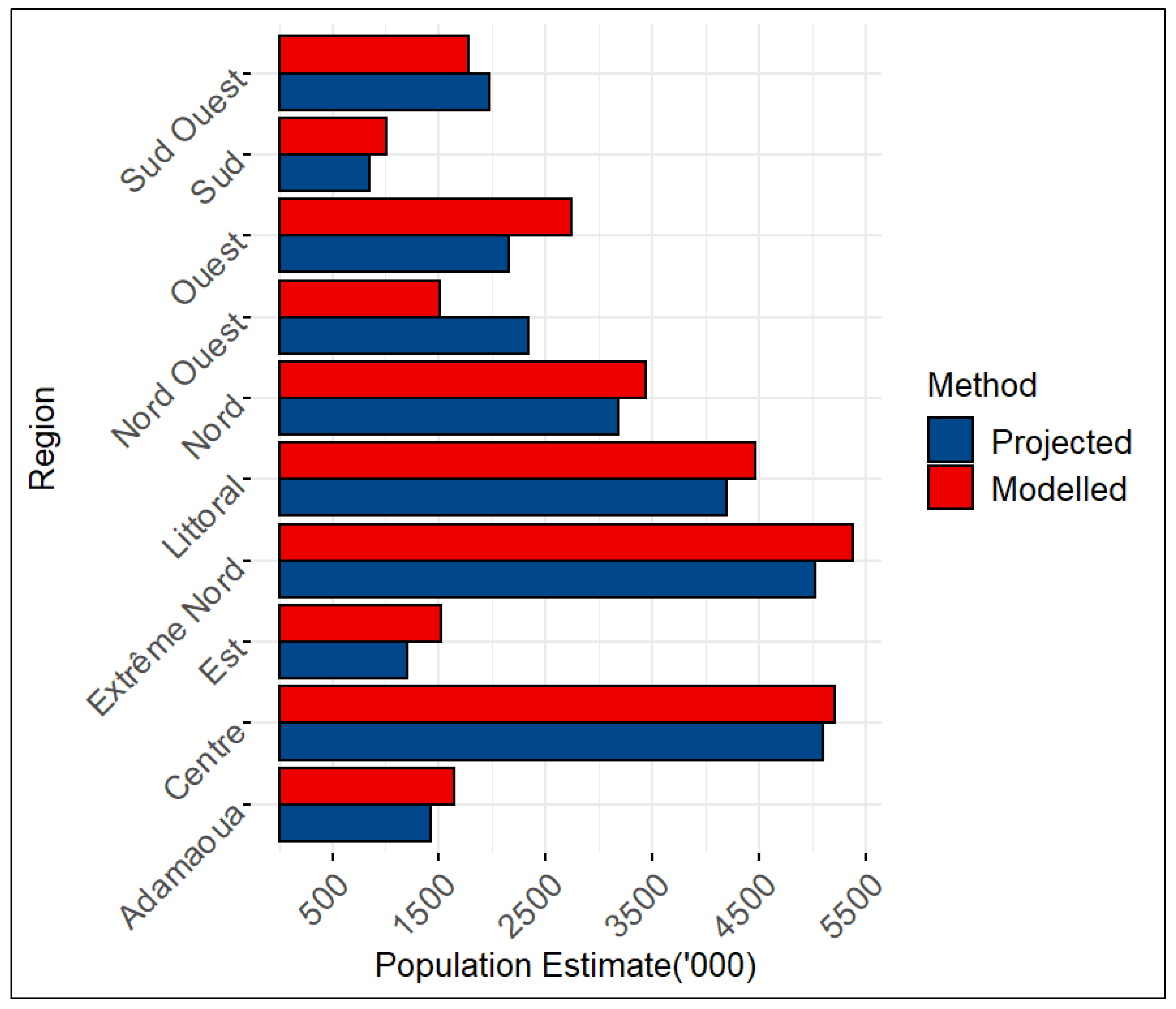
The last population and housing census in Cameroon was in 19 years ago in 2005 and since then, official population data for Cameroon have been provided through projections that use the 2005 census as the baseline. The projections were made using the cohort component approach (Preston et al., 2001). In
Figure 7, we compare the 2022 official projections received from the Cameroon National Institute of Statistics (NIS) with the modelled estimates produced from our methodology for administrative unit 1 (regions). Given the different input data sources and modelling approaches used, we do not expect the output population estimates to agree, but the comparisons can be informative.
Notably, apart from the Nord Ouest and Sud Ouest regions, all of the regions showed slightly higher modelled estimates than the official projections. The lower modelled estimates for the Nord Ouest and Sud Ouest regions could be a result of prolonged high rates of conflicts and insecurity within the regions, thereby leading to high rates of displacement and out-migration that were not accounted for in the cohort component projections.
One key strength of the modelling approach outlined here is that it takes advantage of more recent small area population data and geospatial covariates that can capture recent changes in population distributions and associated drivers, unlike the cohort component population projection approach used by the NIS. This feature of our modelling approach has led the Cameroon NIS to adopt the modelled estimates in supporting census preparation and as a sample frame in the design and implementation of health campaigns.
The full datasets have been published online and can be download freely from WorldPop data repository.
Discussions
In this paper, we presented statistical population modelling method that allowed for the integration of multiple data sources as well as spatial autocorrelation within a bottom-up population modelling framework (e.g., Leasure et al., 2020; Boo et al., 2022; Darin et al, 2022; Nnanatu et al., 2024). For an improved computational efficiency and higher accuracy, we adapted the integrated nested Laplace approximation (INLA; Rue et al. 2009) statistical modelling technique, in conjunction with the stochastic partial differential equation (SPDE; Lindgren et al. 2011) strategies. Bayesian statistical framework enabled us to integrate prior information whilst simultaneously estimating the hierarchical regression model parameters along with their uncertainties.
The methodology was successfully validated using both an extensive simulation study and real data application. The aim of the simulation study was to evaluate the robustness of the methodology over different combinations of missing data proportions and spatial autocorrelation (spatial variance). Model performance in terms of prediction accuracy increased with lower proportion of missing data values and higher spatial autocorrelation. As a proof of concept, small area estimates of population were produced for Cameroon using 5 nationally representative household listing datasets. Modelled estimates were validated using k-fold cross-validation while model selection was based on the deviance information criterion (DIC; smaller values indicated better fit models).
However, it is important to highlight the key limitations of our methodology: First, within the simulation study, we only the scenario where the different data sources do not differ significantly in terms of their data collection designs. Although, this was the case in the motivating dataset where all five data sources used the same sampling strategy. The data source random effect was found not to be statistically significant in preliminary studies and so it was not included in the later models. However, in contexts where data are collated from different sources with significantly different data collection strategies, it makes sense to explore the potential effects of different levels of data source variabilities using an extensive simulation study. Also, the use of household listing datasets and geospatial covariates from different years without explicitly accounting for the year difference effects, and the various sampling frames is likely to be a source of variability that needs to be investigated in future studies. Additionally, temporarily displaced populations due to insecurity may affect population estimates when building footprints are used as a covariate. These aspects will be explored further in future studies.
Nevertheless, the methodology presented here is an important development within the context of population modelling and will serve to provide more accurate small area population data required to address several population data gaps across many countries. Our modelling approach draws upon more recent small area population data and geospatial covariates to estimate population numbers at unsampled locations thereby capturing recent drivers of population changes/density and distributions. As noted, this is a key strength of our approach over the commonly used population projection methods like the cohort component population projection method (e.g., Smith et al., 2013). These datasets which were produced in close collaboration with the Cameroon National Institute of Statistics are publicly available (
https://data.worldpop.org/repo/wopr/CMR/population/v1.0/) and now being used by the Cameroon NIS in supporting census preparation and as a sample frame in the design and implementation of health campaigns in Cameroon.
Author Contributions
Conceptualization: CCN; Data Curation: ANL, ADD, OY, CCN; Formal Analysis: CCN, OY, TA, AG; Methodology: CCN; Project Administration: ANL, AJT; Software: CCN; Supervision: ANL, AJT; Writing - original draft: CCN; Writing – review & editing: AJT, CCN, OY, TA, AG, ANL, ADD.
Acknowledgments
We are grateful to the Cameroon National Institute of Statistics (NIS) for providing the household listing datasets, and the projected population estimates used in this research. We appreciate Edith Darin for reviewing the initial draft of manuscript, we thank the Spatial Statistical Modelling (SSPM) team for their very constructive comments on the initial drafts. This work is part of the GRID3 (Geo-Referenced Infrastructure and Demographic Data for Development) program funded by the Bill and Melinda Gates Foundation and the United Kingdom Foreign, Commonwealth & Development Office (OPP1182425). Project partners include WorldPop at the University of Southampton, the United Nations Population Fund (UNFPA), Center for Integrated Earth Science Information (CIESIN) in the Columbia Climate School at Columbia University, and the Flowminder Foundation.
Conflicts of Interest
The authors declare that they have no known competing financial interests or personal relationships that could have appeared to influence the work reported in this paper.
Ethics statements
The datasets utilised in this study were completely anonymised and aggregated to avoid confidentiality issues in accordance with relevant data protection regulations. Additionally, Ethical approval was obtained from the University of Southampton; ethics approval number: ERGO II 72177 (GRID3 - Cameroon pre-EA tool application)
References
- Anselin, L. Spatial dependence and spatial structural instability in applied regression analysis. Journal of Regional Science 1990, 30, 185–207. [Google Scholar] [CrossRef]
- Bakka, H.; Rue, H.; Fuglstad, G-A.; et al. Spatial modeling with R-INLA: A review. WIREs Comput Stat 2018, 10, e1443. [Google Scholar] [CrossRef]
- Boo, G.; Darin, E.; Leasure, D. R.; Dooley, C. A.; Chamberlain, H. R.; Lazar, A. N.; Tschirhart, K.; Sinai, C.; Hoff, N. A.; Fuller, T.; Musene, K.; Batumbo, A.; Rimoin, A. W.; Tatem, A. J. High-resolution population estimation using household survey data and building footprints. Nature Communications 2022, 13, 1330. [Google Scholar] [CrossRef] [PubMed]
- Chamberlain, H. R.; Darin, E.; Adewole, W.A.; Jochem, W.C.; Lazar, A.N.; Tatem, A.J. Building footprint data for countries in Africa: to what extent are existing data products comparable? Comput. Environ. Urban Syst. 2024, 110, 102104. [Google Scholar] [CrossRef]
- Chan-Golston, A.; Banerjee, S.; Belin, T.R.; et al. Bayesian finite-population inference with spatially correlated measurements. Jpn J Stat Data Sci 2022, 5, 407–430. [Google Scholar] [CrossRef]
- Chi, G.; Voss, P.R. Small-area population forecasting: borrowing strength across space and time. Population, Space, and Place. 2011, 17, 505–520. [Google Scholar] [CrossRef]
- Cressie, N. Statistics for spatial data, rev. ed.; Wiley: New York, 1993. [Google Scholar]
- Darin, E.; Kuépié, M.; Bassinga, H.; Boo, G.; Tatem, A. J. La population vue du ciel : quand l’imagerie satellite vient au secours du recensement. Population 2022, 77, 467–494. [Google Scholar] [CrossRef]
- Diggle, P.J.; Giorgi, E. Model-Based Geostatistics for Prevalence Mapping in Low-Resource Settings. Journal of The American Statistical Association 2016, 515, 111. [Google Scholar] [CrossRef]
- Dooley, C. A.; Leasure, D.R.; Boo, G.; Tatem, A.J. Gridded maps of building patterns throughout sub-Saharan Africa, version 2.0. University of Southampton: Southampton, UK. Source of building footprints “Ecopia Vector Maps Powered by Maxar Satellite Imagery”© 2020/2021. 2021. [Google Scholar] [CrossRef]
- Ecopia and Digital Globe. Technical specification: Ecopia building footprints powered by DigitalGlobe. 2017. Available online: https://dg-cms-uploads-production.s3.amazonaws.com/uploads/legal_document/file/109/DigitalGlobe_Ecopia_Building_Footprints_Technical_Specification.pdf (accessed on 11 April 2022).
- Giorgi, E.; Diggle, P.J.; Snow, R.W.; Noor, A.M. Geostatistical Methods for Disease Mapping and Visualisation Using Data from Spatio-temporally Referenced Prevalence Surveys. Int Stat Rev 2018, 86, 571–597. [Google Scholar] [CrossRef]
- Gomez-Rubio, V. Bayesian inference with INLA; Boca Raton: CRC PressCRC Press: Boca Raton, 2020; Available online: https://becarioprecario.bitbucket.io/inla-gitbook.
- James, G.; et al. An Introduction to Statistical Learning, 1st ed.; Springer: Germany, 2013. [Google Scholar]
- Leasure, D. R.; Jochem, W.C.; Weber, E. M.; Seaman, V.; Tatem, A.J. National population mapping from sparse survey data: A hierarchical Bayesian modeling framework to account for uncertainty. Proceedings of the National Academy of Sciences 2020, 117, 24173–24179. [Google Scholar] [CrossRef]
- Lindgren, F.; Rue, H.; Lindström, J. An explicit link between Gaussian fields and Gaussian Markov random fields: The stochastic partial differential equation approach. Journal of the Royal Statistical Society: Series B (Statistical Methodology) 2011, 73, 423–498. [Google Scholar] [CrossRef]
- McCullagh, P.; Nelder, J. A. Generalized Linear Models, 2nd ed.; Hall/CRC: Chapman, 1989. [Google Scholar]
- Moran, P.A.P. Notes on Continuous Stochastic Phenomena. Biometrika 1950, 37, 17–23. [Google Scholar] [CrossRef] [PubMed]
- National Institute of Statistics. Projections Démographiques et Estimations des Cibles Prioritaires des Différents Programmes et Interventions de Santé. Ministère de la Santé Publique, Cameroon, June 2016. 144 pages. 2016. Available online: https://ins-cameroun.cm/en/statistique/projections-demographiques-et-estimations-des-cibles-prioritaires-des-differents-programmes-et-interventions-de-sante/.
- Nieves, J. J.; Stevens, F. R.; Gaughan, A. E.; Linard, C.; Sorichetta, A.; Hornby, G.; Patel, N. N.; Tatem, A. J. Examining the correlates and drivers of human population distributions across low- and middle-income countries. J. R. Soc. Interface 2017, 14, 20170401. [Google Scholar] [CrossRef] [PubMed]
- Nnanatu, C.C.; Bonnie, A.; Joseph, J.; Yankey, O.; Cihan, D.; Gadiaga, A.; Voepel, H.; Abbott, T.; Chamberlain, H.; Tia, M.; Sander, M.; Davis, J.; Lazar, A.; Tatem, A.J. Small area population estimation from health intervention campaign surveys and partially observed settlement data. Research Square (Preprint) 2014. [Google Scholar] [CrossRef]
- Paige, J.; Fuglstad, G-A.; Riebler, A.; Wakefield, J. Spatial aggregation with respect to a population distribution: Impact on inference. Spatial Statistics 2022, 52, 100714. [Google Scholar] [CrossRef] [PubMed]
- Pettit, L.I. The Conditional Predictive Ordinate for the Normal Distribution. Journal of the Royal Statistical Society. Series B (Methodological) 1990, 52, 175–84. [Google Scholar] [CrossRef]
- Preston, S.H., P. Heuveline. Demography: Measuring and Modeling Population Processes; Wiley: New York, 2001. [Google Scholar]
- Rue, H.; Held, L. Gaussian Markov random fields. In Theory and applications. Chapman & Hall. 2005. [Google Scholar]
- Rue, H.; Martino, S.; Chopin, N. Approximate Bayesian Inference for Latent Gaussian Models by Using Integrated Nested Laplace Approximations. Journal of the Royal Statistical Society, Series B 2009, 71, 319–92. [Google Scholar] [CrossRef]
- Schiavina, M.; Melchiorri, M.; Pesaresi, M.; Politis, P.; Freire, S.; Maffenini, L.; Florio, P.; Ehrlich, D.; Goch, K.; Tommasi, P.; Kemper, T. GHSL Data Package 2022; Publications Office of the European Union: Luxembourg, 2022; ISBN 978-92-76-53071-8. JRC 129516. [Google Scholar] [CrossRef]
- Simpson, D. P.; Rue, H.; Riebler, A.; Martins, T. G.; Sørbye, S. H. Penalising model component complexity: A principled, practical approach to constructing priors (with discussion). Statistical Science 2017, 32, 1–28. [Google Scholar] [CrossRef]
- Smith, S.K.; Tayman, J.; Swanson, D.A. Overview of the Cohort-Component Method. In A Practitioner's Guide to State and Local Population Projections; The Springer Series on Demographic Methods and Population Analysis; Springer: Dordrecht, 2013; Volume 37. [Google Scholar] [CrossRef]
- Tatem, A.J. Small area population denominators for improved disease surveillance and response. Epidemics 2022, 41, 100641. [Google Scholar] [CrossRef] [PubMed]
- Tobler, W. R. A computer movie simulating urban growth in the Detroit region. Economic Geography 46 S 1970, 46 S1, 234–240. [Google Scholar] [CrossRef]
- UNFPA. “The value of modelled population estimates for census planning and preparation.” Technical Guidance Note, August 2020 (updated version 2). 2020. Available online: https://www.unfpa.org/resources/value-modelled-population-estimates-census-planning-and-preparation.
- Wakefield, J. Disease mapping and spatial regression with count data. Biostatistics 2007, 8, 158–183. [Google Scholar] [CrossRef] [PubMed]
- Wardrop, N.A.; Jochem, W.C.; Bird, T.J.; Chamberlain, H.R.; Clarke, D.; Kerr, D.; Bengtsson, L.; Juran, S.; Seaman, V.; Tatem, A.J. Spatially disaggregated population estimates in the absence of national population and housing census data. Proceedings of the National Academy of Sciences 2018, 115, 3529–3537. [Google Scholar] [CrossRef]
- Watanabe, S. A Widely Applicable Bayesian Information Criterion. Journal of Machine Learning Research 2013, 14, 867–97. [Google Scholar]
- WorldPop and Institut National de la Statistique et de la Démographie du Burkina Faso. 2022. Census- based gridded population estimates for Burkina Faso 2019, version 1.1. WorldPop, University of Southampton. [CrossRef]
|
Disclaimer/Publisher’s Note: The statements, opinions and data contained in all publications are solely those of the individual author(s) and contributor(s) and not of MDPI and/or the editor(s). MDPI and/or the editor(s) disclaim responsibility for any injury to people or property resulting from any ideas, methods, instructions or products referred to in the content. |
© 2025 by the authors. Licensee MDPI, Basel, Switzerland. This article is an open access article distributed under the terms and conditions of the Creative Commons Attribution (CC BY) license (http://creativecommons.org/licenses/by/4.0/).