
Submitted:
09 October 2025
Posted:
10 October 2025
You are already at the latest version
Abstract
Climate change and rising temperatures in cities as a result of the Urban Heat Island (UHI) are increasing heat stress and forcing the development of efficient, sustainable outdoor cooling systems. The aim of this article was to analyse the integration of adiabatic air cooling systems with photovoltaic (PV) installations in the context of improving thermal comfort and energy autonomy. The study was carried out on the example of a bus station in Rzeszów (Poland), considering two variants of systems: indirect evaporative cooling (PKW/PV-CP-KW) and direct evaporative cooling (BKW/PV-CP-KW). Four levels of the upper limit of thermal comfort (TEmax = 22°C, 22.9°C, 24°C, 25°C) were considered to assess the impact of comfort parameters on the number of hours of system operation, energy consumption and operating costs. The results indicate that raising the TEmax reduces system uptime and significantly reduces the need for cooling – for example, increasing the TEmax from 22.9°C to 24°C reduces usable energy by 41%. At TEmax = 25°C, the BKW system achieves full energy autonomy, it is fully powered by PV. A Life Cycle Analysis (LCA) and Operating Cost of Ownership (LCC) confirmed the environmental and economic benefits of using higher TEmax values. The study highlights the potential of adiabatic cooling systems, in cooperation with a local PV installation, as an adaptive solution, improving thermal comfort in urban space with minimal grid energy consumption.
Keywords:
adiabatic cooling
; photovoltaics
; outdoor thermal comfort
; urban heat island (UHI)
; energy autonomy
; LCA
; LCC
; sustainability
1. Introduction
The urban heat island (UHI) phenomenon poses a significant public health challenge, particularly in cities with intensive development, limited vegetation and high population density. High temperatures in urban areas are associated with increased morbidity due to cardiac and respiratory causes, as well as mental and social problems. For instance, a study of participants in the UK Biobank revealed that an increase in UHI intensity during the summer was linked to a higher risk of mental health issues, such as depression and anxiety [1,2].
In recent years, the issue of human thermal comfort has also received increasing attention. So far, this concept has mainly been analysed in relation to enclosed spaces. However, the dynamic development of cities and the increased use of public spaces (e.g. transport hubs, promenades and recreational areas) means that there are growing expectations regarding microclimatic conditions in outdoor environments too [3,4]. Therefore, thermal comfort in open spaces is not only a matter of subjective comfort, but also affects mobility and the attractiveness of urban spaces, as well as the psychophysical well-being of residents [5].
In addition, technological and design advances mean that an increasing proportion of the population, particularly in developed countries, expects the same level of microclimate regulation outdoors as indoors. This is due to growing health awareness and socio-cultural processes that contribute to higher quality of life standards in cities. Furthermore, the observed increase in heatwaves means that ensuring thermal comfort in public spaces is not only an element of urban attractiveness, but also a requirement for adapting to climate change [6,7,8,9].
Therefore, literature increasingly emphasises the need to design cooling systems for outdoor spaces. In addition to health functions, these systems would respond to growing social expectations regarding urban environment quality [10]. These solutions include natural and artificial methods, and the choice depends on local climatic and infrastructural conditions, as well as the social preferences of users. The first group consists of solutions such as the development of green infrastructure, the use of high-albedo materials to reduce solar absorption and proper urban design, with an emphasis on creating shaded public spaces [11,12,13,14,15,16]. The second group includes technical solutions related to improving energy efficiency and the use of innovative cooling systems [17,18]. The following technologies may be important in the context of outdoor space cooling:
This article aims to expand existing knowledge of adiabatic cooling systems for reducing heat loads in outdoor areas, using a local bus station in Rzeszów, Poland, as an example [25]. The analysis includes proposing alternative end points for the air cooling process. Selecting different end points enables us to identify various cooling capacity demands. Changes in cooling load can significantly impact the system's energy balance, operating costs, and environmental footprint. Another important aspect of the study is the assessment of the synergy between the cooling system and the existing photovoltaic installation, allowing consideration of integration within the concept of hybrid systems. The final objective of the analysis is to identify a cooling endpoint that would ensure the tested system has a high level of energy autonomy, thus aligning with the principles of sustainable development and optimising the operation of building infrastructure.
2. Overview of Existing Adiabatic Cooling Solutions
Adiabatic (evaporative) cooling uses the evaporation of water to lower the temperature of the air. These technologies are found in two main forms:
- direct evaporative cooling (DEC),
- indirect evaporative cooling (IEC),
- hybrid (indirect-direct, IDC),
- in the form of sprinklers/mists.
These systems are energy-efficient because they require less energy than compressor refrigeration systems. However, their efficiency and suitability depend heavily on humidity, water and air quality (e.g. dust and smoke), and sanitary conditions [26,27]. Table 1 summarises the characteristics of each type of adiabatic cooling in tabular form. The technical data are range-based and come from experimental studies and literature reviews [26,27,28,29,30,31,32,33,34,35,36,37,38]. Actual values may vary depending on climatic conditions (e.g. relative humidity and ambient temperature) and installation parameters.
The choice of technology should take into account the local climate, especially air humidity. In humid areas, DEC is not very efficient, whereas IEC or hybrid solutions are preferable when the humidity in the refrigerated space needs to be limited [26,33]. It is crucial to assess air and cooling water quality, as fog and DEC systems can increase exposure to dust and pathogens in polluted air if the systems are not properly serviced. Using systems that suck in air from the outside (in the absence of filtration) during periods of forest fires or high air pollution can be risky for human health [30,35]. Adiabatic systems also require well-defined maintenance plans, including regular maintenance and water management, to minimise sanitary risks and optimise resource consumption [37,39].
3. Synergy of Adiabatic Cooling Systems and Photovoltaics
In temperate climates (including Poland), the demand for cooling outdoor spaces peaks during the hours of maximum solar radiation and direct heat [25]. This daily demand profile coincides with the energy production curve of photovoltaic (PV) installations. This temporal coincidence generates a fundamental prerequisite for integrating PV into cooling systems, including adiabatic cooling: locally available, directly produced solar energy can power pumps and fans, as well as control cooling systems, exactly when they are needed most. This significantly improves energy self-supply and reduces the need for power from the grid [40,41]. The main benefit of using a PV system to power the cooling system is that it reduces the installation's operating costs – some (or all) of the energy needed to operate the pumps/fans comes directly from the PV system, reducing the consumption of energy from the power grid. Secondly, cooling the PV modules (directly or indirectly by cooling the air in their immediate vicinity) lowers the operating temperature of the cells. This counteracts the drop in voltage and power during periods of high panel temperatures in strong sunlight. This translates directly into higher energy production when it is most needed. Empirical and review studies indicate improved output power and efficiency of modules following evaporative cooling or other active PV temperature control methods [42,43].
From an economic point of view, integrating PV with adiabatic cooling systems increases capital expenditure, but generates significant operational savings by:
- reducing electricity consumption from the grid during peak demand hours;
- reduction of costs associated with cooling using traditional devices (e.g. a compressor unit);
- potential extension of the lifespan and increased efficiency of PV modules.
In regions with hot, dry climates, the payback period may be shortened, especially with the additional use of smart controls and minimal energy storage [41,44].
In practice, however, these implementations face significant limitations and challenges, such as:
- variability of weather conditions: sudden cloudiness can limit the temporary production of electricity by PV systems when cooling is needed,
- momentary mismatch: although the shapes of the curves are similar, local weather anomalies may require support systems or energy storage;
- heating of panels through reflected radiation - the impact of PV installations on the microclimate. Large areas of PV installations can alter the local energy balance of the surface and affect the ambient temperature, which should be taken into account in climate and urban analyses [45].
The following design and operational approaches may solve this limitation:
- adaptive control — prioritising the supply of energy to pumps and cooling fans from PV production at peak generation times, using humidity/temperature thresholds and weather algorithms to turn systems on/off [42];
- electricity storage/buffering: short-term energy storage (e.g. batteries or capacitors) with a small capacity can smooth out momentary fluctuations in PV production and ensure critical pump components run for several minutes during periods of obscuration [41];
- hybrid project: combining natural solutions (e.g. trees, shading and high albedo materials) with technical adiabatic cooling systems that work with the PV installation to reduce the overall cooling demand [44];
- economic and climate analysis: modelling the local conjunction of electricity production from PV and cooling demand (time profiles); estimation of investment and operating costs; and emergency scenario modelling, taking into account the risk of smog and fires (limitations on the use of fog in high air pollution).
The convergence of the maximum insolation and the highest demand for external cooling creates a practical and economical basis for integrating photovoltaic (PV) installations with adiabatic cooling systems. Such integration can significantly improve the energy self-sufficiency of cooling solutions, reduce operating costs and boost the efficient electricity production of PV cells by lowering module temperatures. However, intelligent control, short-term energy buffering and hybrid approaches that combine technical technologies and environmental conditions are necessary to achieve optimal results..
4. Object of Research
4.1. Characteristics of the Test Object
The analysis presented in this article refers to the research object characterised in detail in publication [25]. This is the bus station platform in Rzeszów, Poland, which is an open outdoor space (Figure 1). Key operational and architectural parameters are summarised in Table 2. A notable feature of the research area is its roof, which is made of photovoltaic modules and allows the cooling system to be integrated with a local renewable energy source.
4.2. Selection of Cooling System Variants
As part of this analysis, two variants of refrigeration installation were considered which received the highest scores in the criteria of energy efficiency, economic profitability and environmental impact, according to the results of the research [25]. Both solutions are based on adiabatic cooling technology and have been integrated into a functioning photovoltaic installation. The cooling mechanism can be implemented in two configurations:
- PKW/PV-CP-KW variant: indirect cooling using the evaporation effect without affecting air humidity. This process involves a central device generating cooled air, which is transported via a ventilation duct system and distributed to occupied areas via air supply grilles (Figure 2).
- BKW/PV-CP-KW variant: direct evaporative cooling implemented using evaporative air conditioners. In this solution, air is cooled and humidified simultaneously and supplied directly to the usable space via a short channel (Figure 3).
Water is the primary cooling agent for these devices, while electricity is only required to power the fan and circulation pump. Table 3 summarises the technical parameters of the adopted devices.
5. Research Methodology
5.1. Determination of Thermal Comfort Parameters
The analysis used meteorological data on outdoor air parameters from the Rzeszów–Jasionka meteorological station in Poland, which is located at the geographical coordinates 50°06′N, 22°03′E. These data, made available by the Institute of Meteorology and Water Management in Warsaw, include daily and hourly series covering key atmospheric parameters, such as air temperature, relative humidity and wind speed. These parameters were recorded between 2012 and 2019.
Thermal comfort assessment indicators are used to evaluate the thermal load on the human body. Over the past few decades, a number of indicators based on human heat balance have been developed. These differ in terms of the complexity of the calculations, the input data requirements and the degree to which they are suited to external conditions. The following indicators are most often used in field research and numerical simulations [47,48,49,50]:
- PET (Physiological Equivalent Temperature);
- UTCI (Universal Thermal Climate Index).
- PMV (Predicted Mean Vote).
Against the background of the above indicators, the effective temperature (TE) according to Missenard could play a significant role in field studies [51]. Its main advantages are the simplicity of the calculations and the limited input requirements. As it does not require complex data on solar radiation or anthropometric parameters to be taken into account, this indicator is easy to use in field research, especially where the availability of measurement equipment is limited.
Taking the above arguments into account, the range of thermal comfort outdoors for the purposes of this analysis was determined using the effective temperature index (TE), which is based on the Missenard formula [51]:
- for w < of 0.3 m/s:
- for w ≥ of 0.3 m/s:
The TE index values were calculated for each hour between 1 June and 31 August from 2012 to 2019, based on real meteorological data [46]. The analysis was limited to the summer months (June, July and August), which are characterised by the highest air temperatures. Temperature and relative humidity data were obtained from the Rzeszów–Jasionka meteorological station, while wind speed values recorded by the anemometer were scaled to a height of 1 m above ground level using the following relationship [53]:
The reference area was defined as the space occupied by people within three bus parking spaces, at a height of 2 metres. In this area, the wind speed was halved at a height of 1 metre above ground level. The aerodynamic roughness coefficient was assumed to have a value of 2 (Z₀ = 2), corresponding to urban areas with a medium development intensity in cities with a population of between 100 and 500 thousand inhabitants [53].
The level of thermal comfort was determined on the basis of the calculated values of the effective temperature index TE (according to dependencies (1) and (2)). The Mikhailov scale was used for classification, distinguishing between categories of human thermal sensation [51]. According to the Mikhailov scale, comfort conditions are in the TE value range of 21–22.9 °C.
This analysis uses a multivariate approach to determine the upper limit of thermal comfort. This allows for a more comprehensive assessment of the impact of weather conditions on cooling demand. As part of the study, four variants of the upper comfort limit were adopted: TEmax = 22°C, TEmax = 22.9°C, TEmax = 24°C, and TEmax = 25°C. This approach enables the sensitivity of cooling systems to the adopted comfort criteria to be analysed, and the hours when it is necessary to start up the refrigeration system to be identified.
Taking into account the various upper comfort limits enables us to determine the point at which the cooling capacity can be generated with the support of the existing photovoltaic system, thereby ensuring the system's energy autonomy. This approach enables the technical parameters of the cooling system to be optimised, ensuring user comfort with minimal energy consumption from the power grid.
5.2. Calculation of Cooling Capacity
The cooling capacity demand was calculated on the assumption that the cold supplied to the analyzed QCH zone should completely balance the total QZC heat gains generated in the outdoor zone. QZC total heat gain consists of two components:
- variable gains (QZC-Z) – calculated on the basis of instantaneous parameters of the outside air;
- fixed profits (QZC−S) – resulting from heat emission by sources present in the examined facility.
The relationship between these quantities is expressed by the equation [25]:
The variable heat gains, resulting from the amount of heat received by the flowing air stream (QZC−Z), were calculated based on the instantaneous parameters of the outside air, using the relationship:
The supply air mass flux was calculated on the basis of the formula:
The volume flow of supply air has been calculated on the basis of:
(Assuming: F = 72 m2).
The starting point of the cooling process (P1) was determined based on the actual parameters of the outdoor air recorded during the hours when cooling was required. The end point of the cooling process (P2) is defined by the air parameters described by T2. The T2 value was calculated by converting dependency (2) into the TE indicator using the following formula:
This analysis is based on the assumption that the value of the T2 parameter can be one of four different values: 22°C, 22.9°C, 24°C or 25°C. The rationale behind this selection is that 22°C corresponds to the 'middle' of the thermal comfort range on the Mikhailov scale [51], whereas 22.9°C marks the upper limit of thermal comfort on the same scale. The values of 24°C and 25°C fall outside the thermal comfort range, but have been considered to determine the point at which the cooling system can operate autonomously using the power generated by the existing PV system.
The constant heat gains observed in the study area are due to people staying in the zone and motor vehicles located in its immediate vicinity. The paper [25] presents a detailed methodology for determining this type of heat gain. The results of the constant heat gain calculations are taken from this publication, and a summary of the values is presented in Table 4.
5.3. Determination of Solar Radiation Potential
To determine the solar radiation potential of the facility under study, an analysis was carried out of the actual electricity yields from the existing photovoltaic installation acting as a roof over the external cooling zone. The technical data for this installation can be found in section 4.1 of this paper. Energy generation by the PV installation was measured through the Energy Management System, which enabled remote monitoring of the system's operation.
For the analysis, the daily electricity yields from June, July and August 2019 were taken into account. Only the days on which cooling was required were selected for the analysis; these were the days on which the effective temperature index exceeded the set limit values for the individual comfort variants (22°C, 22.9°C, 24°C and 25°C).
5.4. Comparative Analysis of the Assumed Variants
5.4.1. Energy Effect
The energy effect of the individual cooling variants was calculated based on the demand for primary, final and useful energy, in accordance with the guidelines set out in paper [54]. The following formulas were used for this purpose:
- annual primary energy demand EP:
- annual final energy demand EK:
- annual usable energy demand EU:
The annual primary energy demand, denoted Qp, signifies the annual non-renewable primary energy demand for the cooling system, defined as Q(p,C).
To determine the annual final energy demand for the cooling system, the following relationship was assumed:
The values of the coefficients employed in the calculation of the energy effect, contingent on the variant of the installation, are presented in Table 5.
5.4.2. Environmental Effect (LCA)
The proposed variants of the air cooling system in the outdoor zone were assessed in terms of environmental impact using life cycle analysis (LCA) in accordance with the standards [55,56]. The Eco-Indicator method was utilised for the assessment, delineating three categories of damage [57,58]: human health, ecosystem quality and natural resources [60,61]. The environmental impact was calculated on the assumption of an egalitarian cultural version and a long-term perspective of technological development. The Eco-Indicator values were calculated for each damage category and each installation variant, with the functional unit defined as the demand for non-renewable primary energy and a lifetime of 25 years. The present analysis is limited to the operation phase; the production and decommissioning of the equipment are not included. The calculations were based on the unit coefficients of the Eco-indicator, referring to GJ of useful energy. The values of the assumed coefficients are presented in Table 6.
5.4.3. Economic Impact (LCC)
The Life Cycle Cost (LCC) method was utilised in order to conduct an economic analysis of selected variants of the cooling installation of the research facility [59,60]. This method encompasses all costs incurred throughout the product life cycle, thereby enabling the comparison of alternative design options and the selection of the optimal solution in terms of total investment and operating costs. The economic analysis in terms of LCC was conducted in this paper using the complex method, according to the formula [59,60]:
The LCC method is predicated on the analysis of discounted cash flows and incorporates various cost elements, including the consumption of useful energy carriers, maintenance and maintenance of the installation, as well as price volatility over the lifetime. Therefore, for each of the analysed variants of the cooling installation, the following were determined: investment costs, ownership costs (including, inter alia, technical inspections, servicing, cleaning, potential repair costs, as well as operating costs related to the consumption of electricity and water from the water supply network), the forecasted increase in the prices of carriers and the lifetime of the investment.
6. Results
6.1. Thermal Comfort Parameters – Range
The following figure illustrates the frequency of situations in which the value of the TE indicator exceeded the thermal comfort range under different assumptions of the upper limit of TE (TEmax). It does so by showing the number of such hourly events that occurred between 2012 and 2019.
Figure 4.
The frequency of episodes when the TE index exceeded the upper limit of thermal comfort in individual years [46].
Figure 4.
The frequency of episodes when the TE index exceeded the upper limit of thermal comfort in individual years [46].
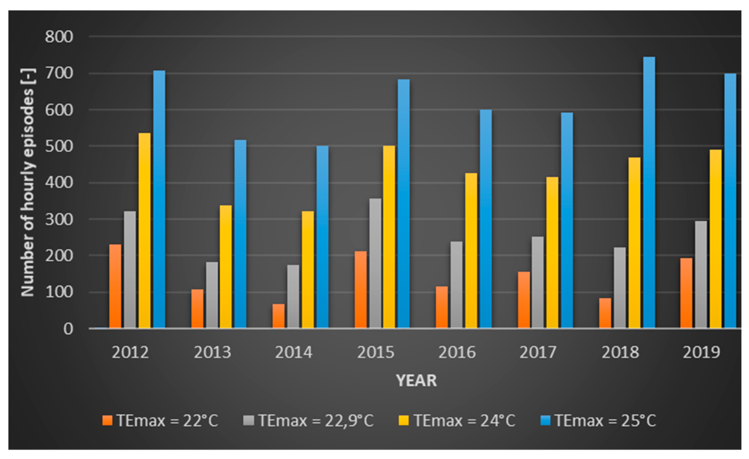
In the outdoor area under consideration, the requirement for cooling is experienced during the summer months, specifically the period spanning from June to August. The months of June, July and August. In the period under analysis (2012-2019), the number of hours per season in which cooling was required, assuming the upper limit of thermal comfort according to the Mikhailov scale (TEmax = 22.9°C), ranged from 332 to 537. This range generally corresponds to several hours per day. However, it should be emphasised that in the coming years the number of such events may increase significantly due to climate change, which further confirms the need to develop air cooling systems in external areas of human habitation.
Furthermore, a substantial discrepancy exists in the requisite duration for cooling, contingent on the established thermal comfort parameters. To illustrate this point, consider the effect of reducing the upper limit of the comfort index from TEmax = 22.9°C to TEmax = 22°C. This results in an increase in the number of cooling hours from 36% in 2014 to as much as 59% in 2018. It is evident that this will result in a substantial augmentation of the cooling system's operational longevity. Consequently, there will be an escalation in the associated operating expenses. The augmentation of the limit to TEmax = 24°C has been demonstrated to result in a reduction in the duration of cooling episodes, with a decline observed from 41% in 2014 to 109% in 2018. Consequently, there has been a substantial decrease in the operational duration of the cooling system, which has resulted in a minor decline in thermal comfort for human subjects.
6.2. Cooling Capacity Demand
The determination of variable heat gains QZC-Z was made on the basis of meteorological data for the area of the research facility and assuming different values of thermal comfort temperature. The calculations were executed in accordance with the methodology delineated in point 5.2 of this document. The total demand for cooling capacity necessary to ensure thermal comfort in the analysed outdoor zone is the sum of the variable heat gains QZC−Z and the constant heat gains QZC−S, determined on the basis of the heat balance and equal to 94 kW. A comprehensive analysis was conducted to ascertain the energy requirements for cooling in each variant, with the operational hours of the air cooling system being a pivotal factor in this analysis. The results of the calculation are displayed in Figure 5.
A thorough analysis of the usable energy has been conducted for the individual variants, indicating that increasing the upper limit of thermal comfort from TEmax = 22.9°C to TEmax = 24°C leads to a significant decline in seasonal usable energy demand, with a reduction of 41% observed (from 48,411 kWh to 28,803 kWh). Conversely, a reduction in the thermal comfort limit by 0.9°C (up to TEmax = 22°C) results in a 42% increase in usable energy, reaching 68,594 kWh.
6.3. Degree of Coverage of Energy Needs from PV Installations
The degree of energy demand coverage by the cooling system in relation to the different variants of the upper limit of thermal comfort (cooling end point) is presented, based on the actual daily electricity yields from the existing PV installation in 2019. The results are presented in Figure 6, Figure 7, Figure 8 and Figure 9. The graphs illustrate the discrepancy between the electricity produced by the PV installation (exceeding the required threshold, indicated by positive values) and the electricity that would need to be imported from the power grid (indicated by negative values). The analysis was conducted on two specific adiabatic air cooling systems: the direct evaporative cooling system (BKW/PV-CP-KW) and the indirect evaporative cooling system (PKW/PV-CP-KW).
The graphs (Figure 6, Figure 7, Figure 8 and Figure 9) show how the proportion of electricity demand for cooling purposes produced by a local PV installation changes. With an assumed upper limit of thermal comfort of TEmax = 22°C, the existing photovoltaic installation can cover 81% of energy needs for the BKW/PV-CP-KW installation and 77% for the PKW/PV-CP-KW system. Increasing the upper limit of thermal comfort towards higher TEmax values significantly increases the degree of coverage of energy needs for cooling. According to the Mikhailov scale (TEmax = 22.9°C), the coverage is 87% for the BKW/PV-CP-KW installation and 83% for the PKW/PV-CP-KW system. Increasing TEmax by 1.1°C results in 98% coverage of the electricity demand from PV for the BKW/PV-CP-KW installation and 91% for the PKW/PV-CP-KW system. The existing PV installation is only able to cover 100% of the electricity demand for the direct evaporative cooling variant (BKW/PV-CP-KW) and 97% for indirect evaporative cooling (PKW.PV-CP-KW) when the upper limit of thermal comfort is shifted to TEmax = 25°C. This value can be considered the autonomy limit of the analysed cooling system.
6.4. Energy Effect
Based on an analysis of selected air cooling system variants in the outdoor zone and different upper limits of thermal comfort, the seasonal demand for final (EC) and primary (EP) energy was calculated, taking into account the energy effect. The EK and EP values are shown in Figure 10).
The EU usable energy index is the same for both proposed cooling systems because it depends on the upper limit of the cooling range, i.e. the TEmax indicator. The lowest final, usable and primary energy requirements were recorded for the variants with the highest upper thermal comfort limit, i.e. TEmax = 25 °C. This is evident for both analysed cooling systems. At this limit, the direct evaporative cooling system (BKW/PV-CP-KW) achieves an EP value of 0, meaning there is no use of primary energy from renewable sources. Regarding the individual thermal comfort limits, reducing the TEmax value from 22.9 °C to 22 °C increases the EP index value by 91% for the BKW/PV-CP-KW system and by 106% for the PKW/PV-CP-KW system. Changing the TEmax target value to TEmax = 24 °C results in a 41% decrease in EU and EK for both cooling system variants, while EP decreases by 68% for BKW/PV-CP-KW and by 91% for PKW/PV-CP-KW. A similar downward trend is observed in the final energy index (EK), which depends on the efficiency of the selected system, for both systems with an increase in the value of the upper limit of thermal comfort (TEmax).
6.5. Environmental Effect - LCA
The Eco-indicator values were calculated for the adopted variants of air cooling system installation in the outdoor zone and for different thermal comfort limits, in relation to individual environmental impact categories, which were then grouped into corresponding damage categories. Figure 11 shows the impact category indicator values for the individual installation variants, which significantly impact the final Eco-indicator value.
The total value of the Eco-indicator for the analysed cooling installation variants is significantly impacted by the consumption of fossil fuels and the emission of inorganic compounds and carcinogens, as well as climate change and ecotoxicity. Studies on various cooling systems have shown that the selected variants have a minimal environmental impact. This is because these installations use a small amount of electricity and a natural refrigerant (water) to generate cooling.
An impact analysis of different cooling endpoint values showed that increasing the upper limit of thermal comfort reduces the environmental impact of the cooling system. For both analysed variants, lowering the thermal comfort limit from TEmax = 22.9 °C to TEmax = 22 °C was observed to result in an increase in environmental impact of around 100%. Conversely, raising this value to 24 °C led to a tenfold decrease in environmental impact for the BKW/PV-CP-KW variant and a more than threefold decrease for the PKW/PV-CP-KW system. When TEmax was set to 25°C, there were no negative environmental impacts for direct evaporative cooling and only minimal effects for indirect adiabatic cooling.
Figure 12 illustrates the changes in the Eco-indicator value for each category of damage in the analysed air cooling system variants.
In generalising the values of the eco-indicators of the individual impact categories to broader categories of damage, it can be concluded that operating the proposed variants of air cooling systems primarily affects human health and natural resources, with a much lesser impact on the quality of the ecosystem. Human health is most affected by emissions of inorganic compounds and carcinogens associated with the substances used, and to a lesser extent by climate change. With regard to natural resources, the main environmental burden is the consumption and extraction of fossil fuels.
Impact analysis under different assumptions of the maximum thermal comfort temperature shows a similar tendency towards decreasing impact in individual damage categories, as observed in impact categories. Any change in the assumed target value for cooling temperature results in a corresponding change in the level of impact on all analysed damage categories.
It should be emphasised that the presented analysis only refers to the operational stage of the proposed installation variants, omitting the production, disassembly and final disposal stages of the equipment. Taking the full life cycle of the installation into account would result in higher Eco-Indicator values and a greater estimated impact on the natural environment.
6.6. Economic Effect – LCC
An economic analysis of air cooling variants in the outdoor zone was carried out using the Life Cycle Cost (LCC) method. The calculations took into account the assumptions presented in Table 7.
Unit prices of utilities are presented in Table 8.
The results of the life cycle cost analysis (LCC) showed differences between the individual variants of the outdoor air cooling system, depending on the assumed value of the upper limit of the cooling point (TEmax). Figure 13 shows the LCC values, which are calculated as the sum of acquisition costs and cost of ownership.
Investment costs for the indirect evaporative cooling variant (PKW/PV-CP-KW) remain unchanged regardless of the TEmax coefficient value adopted, as changes only affect the installation's operating time and, consequently, operating costs. Operating costs decrease as the TEmax cooling endpoint value increases. In the case of the direct evaporative cooling variant (BKW/PV-CP-KW), however, an increase in investment costs is observed when the upper limit of thermal comfort exceeds TEmax = 24°C. This is due to a decrease in demand for cooling and, consequently, a decrease in the required cooling capacity and number of devices (fewer evaporative air conditioners).
Operating costs are also showing a downward trend as the value of TEmax increases. The largest decrease (98%) was recorded in the range between TEmax = 22.9°C and TEmax = 24°C for the BKW/PV-CP-KW system. Increasing the cooling endpoint by 1.1°C significantly improves the economic balance of the analysed system and could be a cost-effective solution while only minimally reducing the thermal comfort quality standard..
5. Conclusion
- The results of the research indicate that the upper limit of thermal comfort (TEmax) is one of the key parameters that determine the length of cooling periods. Even minor adjustments to TEmax can lead to substantial variations in the cooling system's operating hours, significantly impacting its energy and economic efficiency.
- The operating hours of the cooling system and the usable energy demand depend heavily on the chosen TEmax value. For example, increasing the upper comfort limit from 22.9°C to 24°C results in a 109% reduction in system uptime and a 41% reduction in usable energy demand.
- An increase in the TEmax value significantly improves the degree to which energy demand is covered by the local photovoltaic installation. Full autonomy of the system has been achieved for TEmax = 25°C (100% for the BKW/PV-CP-KW system and 97% for the PKW/PV-CP-KW system).
- Operating costs decrease as TEmax increases, resulting from shorter operating times and lower demand for cold. The BKW/PV-CP-KW system recorded the largest decrease in operating costs (98%) in the TEmax range of 22.9–24°C. Increasing the cooling endpoint by 1.1°C significantly improves the economic balance while only minimally reducing thermal comfort.
- Increasing the thermal comfort range significantly reduces the environmental impact of the cooling system. Lowering the TEmax from 22.9°C to 22°C increases the environmental impact by around 100%, whereas increasing the TEmax to 24°C decreases it tenfold for the BKW/PV-CP-KW system and by more than a third for the PKW/PV-CP-KW system. No negative effects were observed for direct evaporative cooling at TEmax = 25°C, but only minimal effects were observed for indirect cooling. It should be emphasised that the analysis only covers the operational stage of the systems and omits the production, dismantling and disposal phases of the equipment. Taking the full life cycle (LCA) into account could result in higher Eco Indicator values and a greater environmental impact.
- The results of the calculations depend heavily on local meteorological conditions. To improve the accuracy of the analysis, local measurements of air parameters such as temperature, average radiation temperature, relative humidity, wind speed and insolation are necessary.
- The utilisation of alternative methodologies for the assessment of thermal comfort (e.g. PMV, PET or UTCI indicators) has the potential to engender substantial alterations in the findings of energy, economic and environmental analyses.
- The degree of autonomy of the cooling system also depends on the quality and efficiency of the photovoltaic modules used. The analysis used panels with a service life of several years. Replacing these with more efficient modern modules could significantly boost the system's overall efficiency.
-
The following recommendations are proposed for future research:
- conducting research into how the analysed systems cooperate with electricity storage facilities in order to increase autonomy at lower TEmax values,
- optimisation of system operation by cooling PV cells, which could increase their efficiency,
- extension of the analysis to include the full life cycle of the installation (LCA).
Funding
This research received no external funding.
Data Availability Statement
The original contributions presented in the study are included in the article, further inquiries can be directed to the corresponding author.
Conflicts of Interest
The authors declare no conflicts of interest.
Nomenclature
| A | study area (m2) |
| ci | correction factor depending on cooling system (-) |
| Eel,pom,C | annual support final energy demand for cooling system (kWh year-1) |
| EK | annual final energy demand indicator (kWh m-2 year-1) |
| EP | annual primary energy demand indicator (kWh m-2 year-1) |
| EU | annual usable energy demand indicator (kWh m-2 year-1) |
| F | horizontal airflow area (m2) |
| H | height of study area (m) |
| hw | height of wind meter measurement (m) |
| hZ | height under study Z (m) |
| KN | capital costs (euro) |
| KP | ownership, operating costs (euro) |
| L | length of study area (m) |
| n | lifetime of installation (year) |
| N | number of photovoltaic modules (number) |
| No | number of people staying in study area (-) |
| Pj | unit power of photovoltaic cell (W) |
| q | specific sensible heat (W person-1) |
| QCH | cooling power (kW) |
| QC,nd | annual utility energy demand for cooling (kWh year-1) |
| Qk | annual demand for non-renewable final energy supplied for technical systems (kWh year-1) |
| Qk,C | annual final energy demand for the cooling system (kWh year-1) |
| QL | heat gains from people (kWh) |
| Qu | annual useful energy demand (kWh year-1) |
| QZC | total heat gains for research facility (kWh) |
| QZC-S | constant heat gains calculated on basis of heat balance (kWh) |
| QZC-Z | variable heat gains calculated on basis of heat balance (kWh) |
| RH | relative humidity (%) |
| S | width of study area (m) |
| s | discount rate (%) |
| SEER | average seasonal coefficient of energy efficiency of cooling production (-) |
| SEERref | reference average coefficient of energy efficiency of cold production (-) |
| T | air temperature (°C) |
| T2 | real air temperature to be reached at cooling end point (°C) |
| TE | effective temperature (°C) |
| TEmax | upper limit of thermal comfort according to assumptions (°C) |
| V | volume of study object (m3) |
| w | wind velocity (m s-1) |
| wc | coefficient of non-renewable primary energy input for the generation and delivery of the energy carrier or energy for the cooling system (-) |
| wel | coefficient of input of non-renewable primary energy for the generation and supply of electricity, specific for the annual auxiliary energy demand of the cooling system (-) |
| ww | wind velocity at wind meter height (m s-1) |
| wZ | wind velocity at height Z (m s-1) |
| Z0 | aerodynamic roughness coefficient (-) |
| mass flow rate (kg s−1) | |
| volume flow rate (m3s-1) | |
| Greek Symbols | |
| ηC,d | seasonal average efficiency of cooling distribution from cooling source to cooled area (-) |
| ηC,e | average seasonal efficiency of control and usage of cooling in cooled area (-) |
| ηC,s | seasonal average cooling storage efficiency (-) |
| ηC,tot | seasonal average total efficiency of cooling system (-) |
| ϴ | length of period considered (year) |
| Abbreviations | |
| BKW/PV-CP-KW | a cooling system consisting of indirect evaporative air conditioners (local units), short ventilation ducts and air vents, combined with a photovoltaic installation |
| CP | cool air distribution |
| DEC | direct evaporative cooling |
| EC | heat energy |
| IEC | indirect evaporative cooling |
| KW | air diffuser |
| LCA | life cycle assessment (Pt) |
| LCC | life cycle cost (euro) |
| P1 | starting point of cooling process |
| P2 | end point of cooling process |
| PKW/PV-CP-KW | a cooling system comprising an indirect evaporative air conditioner (central unit) and ventilation ducts and air vents, combined with a photovoltaic installation |
| PV | photovoltaic cells |
| SEN | electricity grid |
| TRM | typical meteorological year |
| UHI | urban heat island |
References
- Bao, Y.; Li, Y.; Gu, J.; Shen, C.; Zhang, Y.; Deng, X.; Han, L.; Ran, J. Urban heat island impacts on mental health in middle-aged and older adults. Environ. Int. 2025, 199, 109470. [Google Scholar] [CrossRef]
- Avashia, V.; Garg, A.; Dholakia, H. Understanding temperature related health risk in context of urban land use changes. Landsc. Urban Plan. 2021, 212, 104107. [Google Scholar] [CrossRef]
- Hou, G.; Kuai, Y.; Yin, L.; Li, Y.; Shu, P. A comprehensive review of thermal comfort related design strategy of semi-outdoor transitional spaces. Energy Build. 2025, 345, 116116. [Google Scholar] [CrossRef]
- Jia, S.; Wang, Y.; Wong, N.H.; Weng, O. A hybrid framework for assessing outdoor thermal comfort in large-scale urban environments. Landsc. Urban Plan. 2025, 256, 105281. [Google Scholar] [CrossRef]
- Marando, F.; Heris, M.P.; Zulian, G.; Udías, A.; Mentaschi, L.; Chrysoulakis, N.; Parastatidis, D.; Maes, J. Urban heat island mitigation by green infrastructure in European Functional Urban Areas. Sustain. Cities Soc. 2022, 77, 103564. [Google Scholar] [CrossRef]
- Sayad, B.; Osra, O.A.; Binyassen, A.M.; Quattan, W.S. Analyzing Urban Climatic Shifts in Annaba City: Decadal Trends, Seasonal Variability and Extreme Weather Events. Atmosphere 2024, 15, 529. [Google Scholar] [CrossRef]
- Zhang, J.; Tu, L.; Wang, X.; Liang, W. Comparison of Urban Heat Island Differences in the Yangtze River Delta Urban Agglomerations Based on Different Urban–Rural Dichotomies. Remote Sens. 2024, 16, 3206. [Google Scholar] [CrossRef]
- Casson, N.; Cameron, L.; Mauro, I.; Friesen-Hughes, K.; Rocque, R. Perceptions of the health impacts of climate change among Canadians. BMC Public Health 2023, 23, 212. [Google Scholar] [CrossRef]
- Zhong, Y.; Li, S.; Liang, X.; Guan, Q. Causal inference of urban heat island effect and its spatial heterogeneity: A case study of Wuhan, China. Sustain. Cities Soc. 2024, 115, 105850. [Google Scholar] [CrossRef]
- Saez, R.A. Assessing the burdens of urban heat: a description of functional, economic and public health impacts of increasing heat in cities. Policy Anal. 2023, 1–23. [Google Scholar] [CrossRef]
- Haeffelin, M.; Ribaud, J.F.; Céspedes, J.; Dupont, J.C.; Lemonsu, A.; Masson, V.; Nagel, T.; Kotthaus, S. Impact of boundary layer stability on urban park cooling effect intensity. EGUsphere 2024, 1777. [Google Scholar] [CrossRef]
- Zhu, Y.; Kensek, K.M. MITIGATING THE URBAN HEAT ISLAND EFFECT: The Thermal Performance of Shade-Tree Planting in Downtown Los Angeles. Sustainability 2024, 16, 8768. [Google Scholar] [CrossRef]
- Peng, L.L.H.; Jim, C.Y. Green-Roof Effects on Neighborhood Microclimate and Human Thermal Sensation. Energies 2013, 6, 598–618. [Google Scholar] [CrossRef]
- Bandurski, M.; Bandurska, H.; Kazimierczak-Grygiel, E.; Koczyk, H. The Green Structure for Outdoor Places in Dry, Hot Regions and Seasons—Providing Human Thermal Comfort in Sustainable Cities. Energies 2020, 13, 2755. [Google Scholar] [CrossRef]
- Pan, Y.; Li, S.; Tang, X. Investigation of Bus Shelters and Their Thermal Environment in Hot–Humid Areas—A Case Study in Guangzhou. Buildings 2024, 14, 2377. [Google Scholar] [CrossRef]
- Nicholson, S.; Nikolopoulou, M.; Watkins, R.; Love, M.; Ratti, C. Data driven design for urban street shading: Validation and application of ladybug tools as a design tool for outdoor thermal comfort. Urban Clim. 2024, 56, 102041. [Google Scholar] [CrossRef]
- Diem, P.K.; Nguyen, C.T.; Diem, N.K.; Diep, N.T.H.; Thao, P.T.B.; Hong, T.G.; Phan, T.N. Remote sensing for urban heat island research: Progress, current issues, and perspectives. Remote Sens. Appl. Soc. Environ. 2024, 33, 101081. [Google Scholar] [CrossRef]
- Babiarz, B.; Krawczyk, D.A.; Siuta-Olcha, A.; Manuel, C.D.; Jaworski, A.; Barnat, E.; Cholewa, T.; Sadowska, B.; Bocian, M.; Gnieciak, M.; Werner-Juszczuk, A.; Kłopotowski, M.; Gawryluk, D.; Stachniewicz, R.; Swięcicki, A.; Rynkowski, P. Energy Efficiency in Buildings: Toward Climate Neutrality. Energies 2024, 17, 4680. [Google Scholar] [CrossRef]
- Wei-Han, C.; Huai-En, M.; Tun-Ping, T. Performance improvement of a split air conditioner by using an energy saving device. Energy Build. 2018, 174, 380–387. [Google Scholar] [CrossRef]
- AL-Hasni, S.; Santori, G. The cost of manufacturing adsorption chillers. Therm. Sci. Eng. Prog. 2023, 39, 101685. [Google Scholar] [CrossRef]
- Halon, T.; Pelinska-Olko, E.; Szyc, M.; Zajaczkowski, B. Predicting Performance of a District Heat Powered Adsorption Chiller by Means of an Artificial Neural Network. Energies 2019, 12, 3328. [Google Scholar] [CrossRef]
- Evaporative Cooling Why It Is Perfect for Your Business. Available online: https://www.seeleyinternational.com/eu/ commercial/evaporative-cooling-europe/ (accessed on 28 September 2025).
- Sajjad, U.; Abbas, N.; Hamid, K.; Abbas, S.; Hussain, I.; Ammar, S.M.; Sultan, M.; Ali, H.M.; Hussain, M.; Rehman, T.; et al. A review of recent advances in indirect evaporative cooling technology. Int. Commun. Heat Mass. Transf. 2021, 122, 105140. [Google Scholar] [CrossRef]
- Mohammed, R.H.; El-Morsi, M.; Abdelazis, O. Indirect evaporative cooling for buildings: A comprehensive patents review. J. Build. Eng. 2022, 50, 104158. [Google Scholar] [CrossRef]
- Barnat, E.; Sekret, R.; Babiarz, B. Cooling of Air in Outdoor Areas of Human Habitation. Energies 2024, 17, 6303. [Google Scholar] [CrossRef]
- Haile, M.G.; Garay-Martinez, R.; Macarulla, A.M. Review of Evaporative Cooling Systems for Buildings in Hot and Dry Climates. Buildings 2024, 14, 3504. [Google Scholar] [CrossRef]
- Black-Ingersoll, F.; de Lange, J.; Heidari, L.; Negassa, A.; Botana, P.; Fabian, M.P.; Scammell, M.K. A Literature Review of Cooling Center, Misting Station, Cool Pavement, and Cool Roof Intervention Evaluations. Atmosphere 2022, 13, 1103. [Google Scholar] [CrossRef]
- Mortensen, K. Review of Evaporative Cooling’s Efficiency and Environmental Value. Ashrae J. 2022, 55–61. Available online: https://spxcooling.com/wp-content/uploads/Review_Evaporative_Cooling_Efficiency.pdf?utm.
- Dhariwal, J.; Manandhar, P.; Bande, L.; Armstrong, P.; Reinhart, F.C. Evaluating the effectiveness of outdoor evaporative cooling in a hot, arid climate. Build. Environ. 2019, 150. [Google Scholar] [CrossRef]
- Sonntag, D.B.; Jung, H.; Harline, R.P.; Peterson, T.C.; Willis, S.E.; Christensen, T.E.; Johnston, J.D. Infiltration of Outdoor PM2.5 Pollution into Homes with Evaporative Coolers in Utah County. Sustainability 2024, 16, 177. [Google Scholar] [CrossRef]
- Wei, Q.; Lu, J.; Xia, X.; Zhang, B.; Ying, X.; Li, L. Performance and Applicability Analysis of Indirect Evaporative Cooling Units in Data Centers Across Various Humidity Regions. Buildings 2024, 14, 3623. [Google Scholar] [CrossRef]
- Kostyák, A.; Szekeres, S.; Csáky, I. The Effect of Indirect Evaporative Cooling Applied to Existing AHU Systems. J. Archit. Eng. 2024. [Google Scholar] [CrossRef]
- Arunkumar, H.S.; Madhwesh, N.; Shenoy, S.; Kumar, S. Performance evaluation of an indirect-direct evaporative cooler using biomass-based packing material. Int. J. Sustain. Eng. 2024, 17, 1. [Google Scholar] [CrossRef]
- Wang, P.; Lu, S.; Wu, X.; Tian, J.; Li, N. Mist Spraying as an Outdoor Cooling Spot in Hot-Humid Areas: Effect of Ambient Environment and Impact on Short-Term Thermal Perception. Buildings 2024, 14, 336. [Google Scholar] [CrossRef]
- Solomon, G.M.; Martinez, N.; Behren, J.; Kaser, I.; Chang, D.; Singh, A.; Jarmul, S.; Miller, S.L.; Reynolds, P.; Heidarinejad, M.; Stephens, B.; Singer, B.C.; Wagner, J.; Balmes, J.R. Evaporative coolers and wildfire smoke exposure: a climate justice issue in hot, dry regions. .Front. Public Health 2025, 13, 1541053. [Google Scholar] [CrossRef]
- Zaki, A.M.; Bargal, M.H.S.; Antar, M.A.; Mokheimer, E.M.A.; Alhems, L.M. Advances in indirect evaporative cooling: principles, integrated cycles, economic insights, and environmental implications. Therm. Sci. Eng. Prog. 2025, 67, 104078. [Google Scholar] [CrossRef]
- Stefaniak, Ł.; Szczęśniak, S.; Walaszczyk, J.; Rajski, K.; Piekarska, K.; Danielewicz, J. Challenges and future directions in evaporative cooling: Balancing sustainable cooling with microbial safety. Build. Environ. 2025, 267, 112292. [Google Scholar] [CrossRef]
- Romero-Lara, M.J.; Comino, F.; Ruiz de Adana, M. Seasonal energy efficiency ratio of regenerative indirect evaporative coolers—Simplified calculation method. Appl. Therm. Eng. 2023, 220, 119719. [Google Scholar] [CrossRef]
- Mihai, V.; Rusu, L. Improving the Ventilation of Machinery Spaces with Direct Adiabatic Cooling System. Inventions 2022, 7, 78. [Google Scholar] [CrossRef]
- Parker, D.; Panchabikesan, K.; Dagostiono, D.; Crawley, D.B.; Lawrire, L. Coincidence of Photovoltaic Electric Generation During Heat Waves: An Example Analysis for Northern Italy. EU PVSEC 2024, 020562–001. [Google Scholar] [CrossRef]
- Kan, X.; Hedenus, F.; Reichenberg, L.; Hohmeyer, O. Into a cooler future with electricity generated from solar photovoltaic. iScience 25 2022, 10, 4208. [Google Scholar] [CrossRef]
- Xue, T.; Wan, Y.; Huang, Z.; Chen, P.; Lin, J.; Chen, W.; Liu, H. Comprehensive Review of the Applications of Hybrid Evaporative Cooling and Solar Energy Source Systems. Sustainability 2023, 15, 16907. [Google Scholar] [CrossRef]
- Ghosh, P.; Wei, X.; Liu, H.; Zhang, Z.; Zhu, L. Simultaneous subambient daytime radiative cooling and photovoltaic power eneration from the same area. Cell Rep. Phys. Sci. 2024, 5, 101876. [Google Scholar] [CrossRef]
- Strobel, M.; Jakob, U.; Streicher, W.; Neyer, D. Spatial Distribution of Future Demand for Space Cooling Applications and Potential of Solar Thermal Cooling Systems. Sustainability 2023, 15, 9486. [Google Scholar] [CrossRef]
- Khan, A.; Anand, P.; Garshasbi, S.; Khatun, R.; Khorat, S.; Hamdi, R.; Niyogi, D.; Santamouris, M. Rooftop photovoltaic solar panels warm up and cool down cities. Nat. Cities 2024, 1, 780–790. [Google Scholar] [CrossRef]
- Institute of Meteorology and Water Management, Institute of Meteorology and Water Management-State Research Institute. Available online: https://www.imgw.pl/ (accessed on 10 October 2022).
- Freitas, C.R.; Grigorieva, E.A. A comprehensive catalogue and classification of human thermal climate indices. Int. J. Biometeorol. 2015, 59, 109–120. [Google Scholar] [CrossRef] [PubMed]
- Błażejczyk, K.; Broade, P.; Fiala, D.; Havenith, G.; Holmer, I.; Jendritzky, G.; Kaampmann, B. UTCI—Nowy wskaźnik oceny obciążeń cieplnych człowieka. Przegląd Geogr. 2010, 82, 49–71. Available online: https://www.researchgate.net/publication/2886 08838_UTCI_-_New_index_for_assessment_of_heat_stress_in_man#fullTextFileContent (accessed on 2 October 2025).
- Błażejczyk, K. UTCI—10 years of applications. Int. J. Biometeorol. 2021, 65, 1461–1462. [Google Scholar] [CrossRef] [PubMed]
- Höppe, P. The physiological equivalent temperature—A universal index for the biometeorological assessment of the thermal environment. Int. J. Biometeorol. 1999, 43, 71–75. [Google Scholar] [CrossRef] [PubMed]
- Barnat, E. Air cooling of the external zones of human residence. Ph.D. Thesis, Rzeszow University of Technology, Rzeszów, Poland, 2023. [Google Scholar]
- Klemm, K. Wind flow in an urban area and opportunities for its use. Pol. Sol. Energy 2010, 2–4, 37–42. [Google Scholar]
- Strzelczyk, P.; Szczerba, Z.; Wozniak, A. Vertical modelling of the wind speed profile in an aerodynamic model. JCEEA 2015, XXXII, 62. [Google Scholar] [CrossRef]
- Regulation of the Minister of Infrastructure and Development of 27 February 2015 on the Methodology for Determining the energy Performance of a Building or Part of a Building and Energy Performance Certificates. Journal of Laws of 18 March 2015, item 376, as Amended. Available online: https://isap.sejm.gov.pl/isap.nsf/DocDetails.xsp?id=WDU20150000376 (accessed on 15 October 2024).
- PN-ENISO14040:2009; Environmental management—Life cycle assessment—Principles and Structure. ISO: Geneva, Switzerland, 2009.
- PN-EN ISO 14044:2009; Environmental management—Life cycle assessment—Requirements and Guidelines. ISO: Geneva, Switzerland, 2009.
- Sekret, R. Environmental aspects of energy supply of buildings in Poland. In E3S Web of Conferences; EDP Sciences: Les Ulis, France, 2018; p. 49. [Google Scholar] [CrossRef]
- Sekret, R. Evaluation of environmental impact on selected heat supply systems of buildings for energy management. Rynek Energii 2019, 1, 48–55. [Google Scholar]
- Bogusz, A. LCC Life Cycle Costs Repository. Efficient public procurement. In Polish, Katowice, Poland 2022. Available online: https://dzp.us.edu.pl/wp-content/uploads/2025/01/Repozytorium-koszty-cyklu-zycia-LCC.pdf (accessed on day month year).
- Bogusz, A.; Polakowski, Ł. Life cycle cost accounting – LCC. In Green Public Procurement – II Handbook; Skowron, M., Ed.; Public Procurement Office: Warsaw, Poland, 2012. [Google Scholar]
Figure 1.
The object of the study – the platform of the Local Railway Station in Rzeszów (Poland).
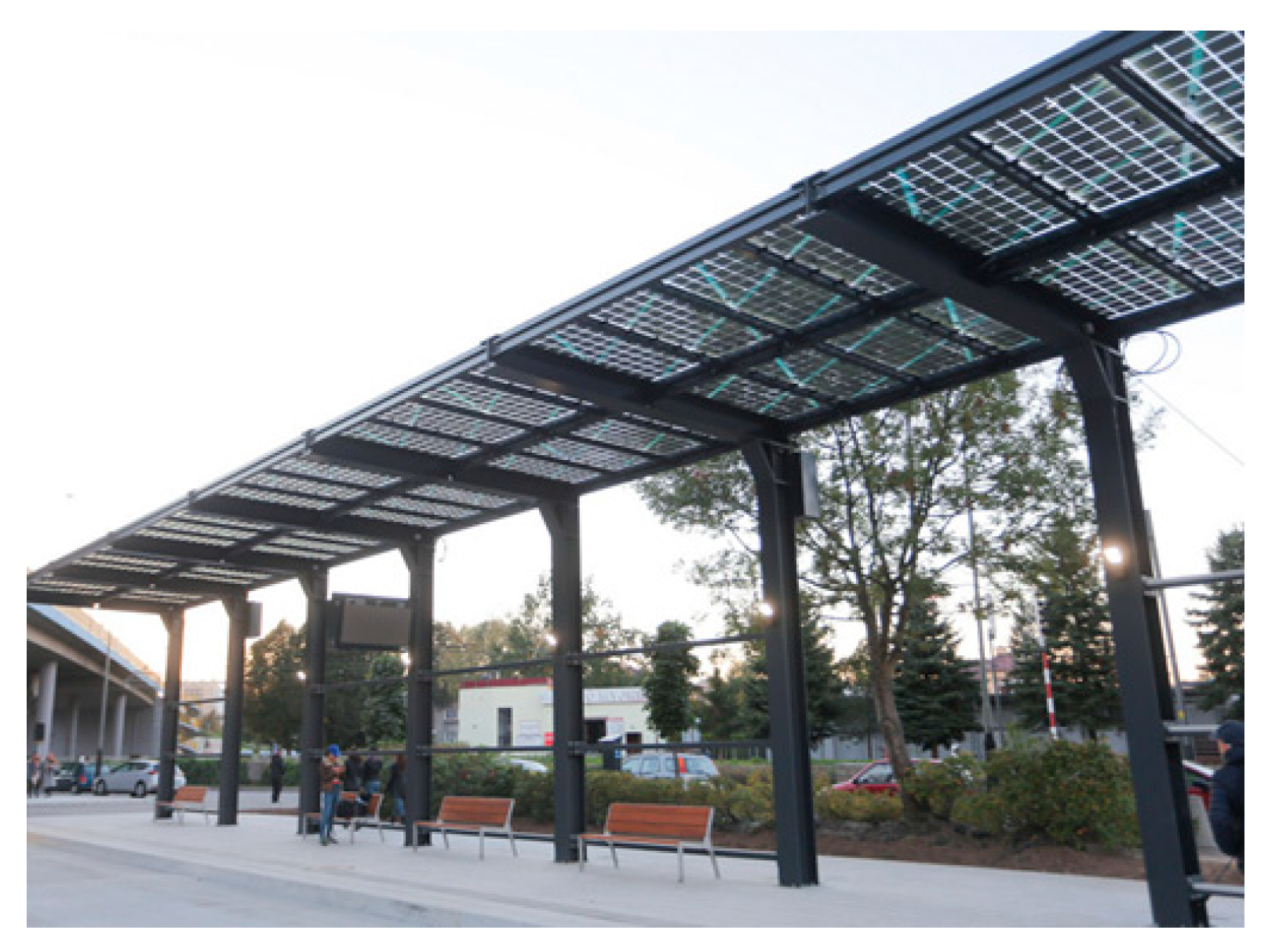
Figure 2.
Diagram of the air cooling system in the PKW/PV-CP-KW variant [25].
Figure 2.
Diagram of the air cooling system in the PKW/PV-CP-KW variant [25].
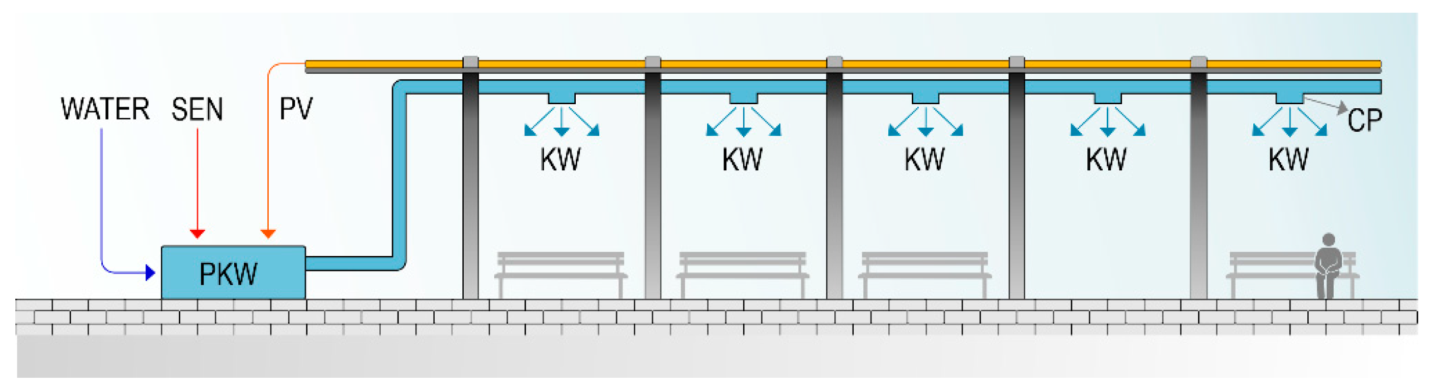
Figure 3.
Diagram of the air cooling system in the BKW/PV-CP-KW variant [25].
Figure 3.
Diagram of the air cooling system in the BKW/PV-CP-KW variant [25].
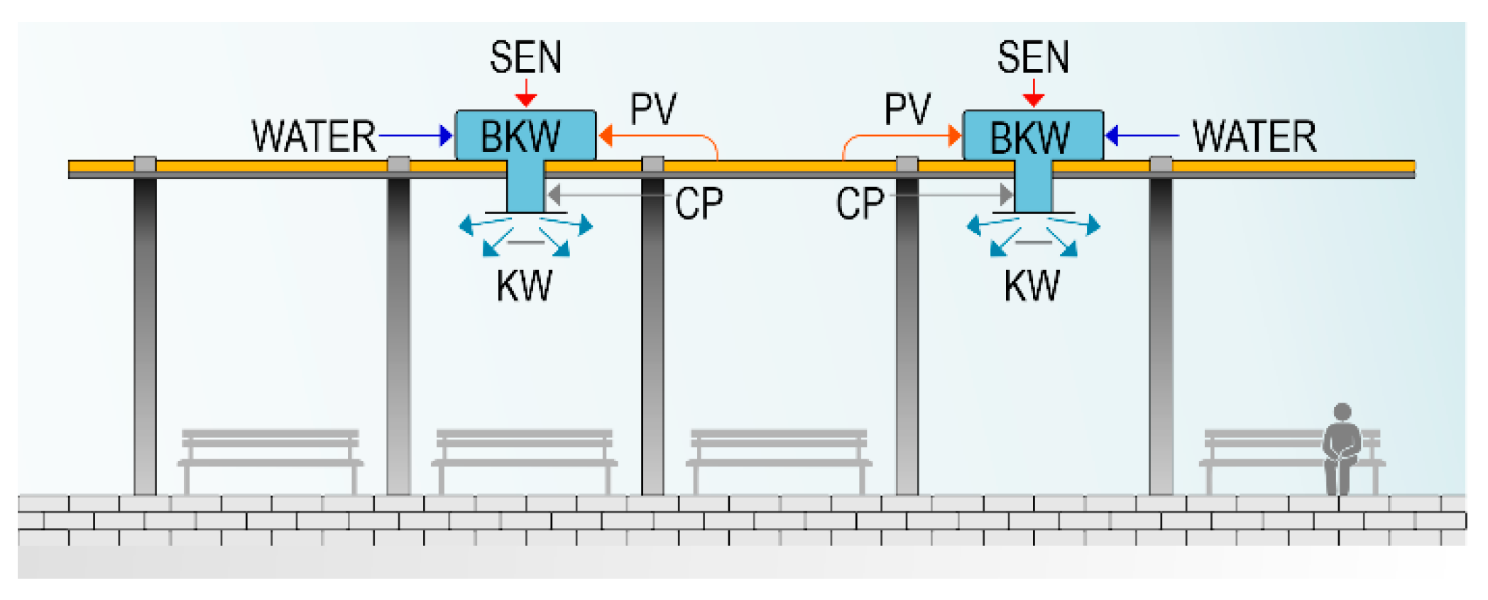
Figure 5.
The usable energy required to generate cooling by the cooling system for the individual variants.
Figure 5.
The usable energy required to generate cooling by the cooling system for the individual variants.
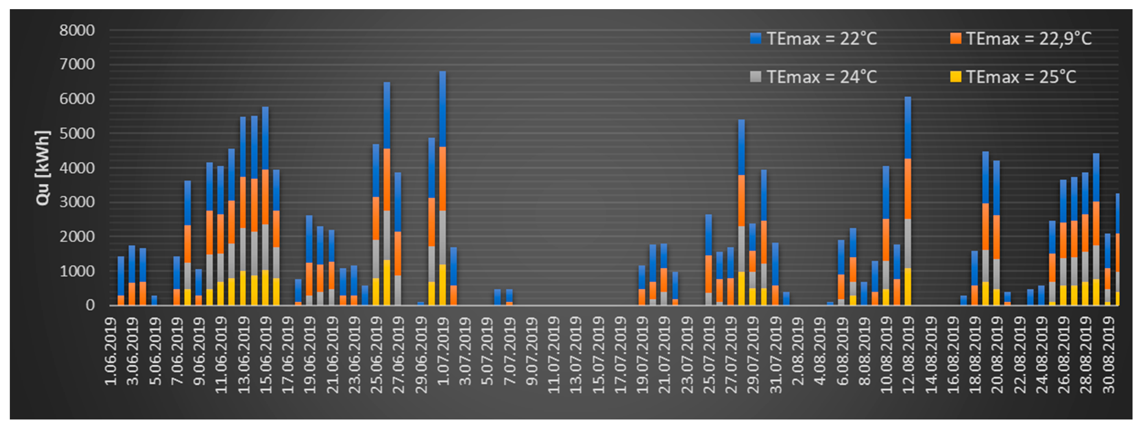
Figure 6.
Excess and daily shortage of electricity produced from the existing PV installation in the case of the upper limit of thermal comfort TEmax = 22°C.
Figure 6.
Excess and daily shortage of electricity produced from the existing PV installation in the case of the upper limit of thermal comfort TEmax = 22°C.
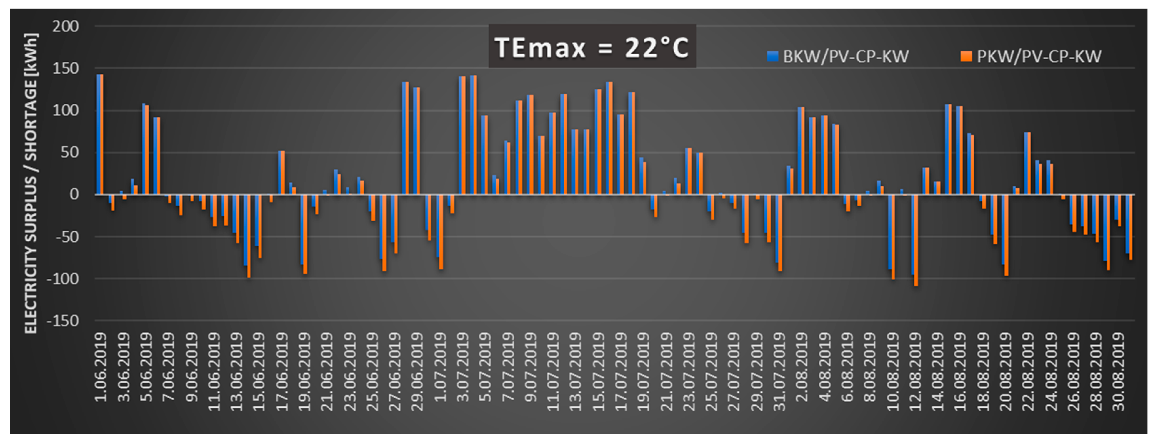
Figure 7.
Excess and daily shortage of electricity produced from the existing PV installation in the case of the upper limit of thermal comfort TEmax = 22.9°C.
Figure 7.
Excess and daily shortage of electricity produced from the existing PV installation in the case of the upper limit of thermal comfort TEmax = 22.9°C.
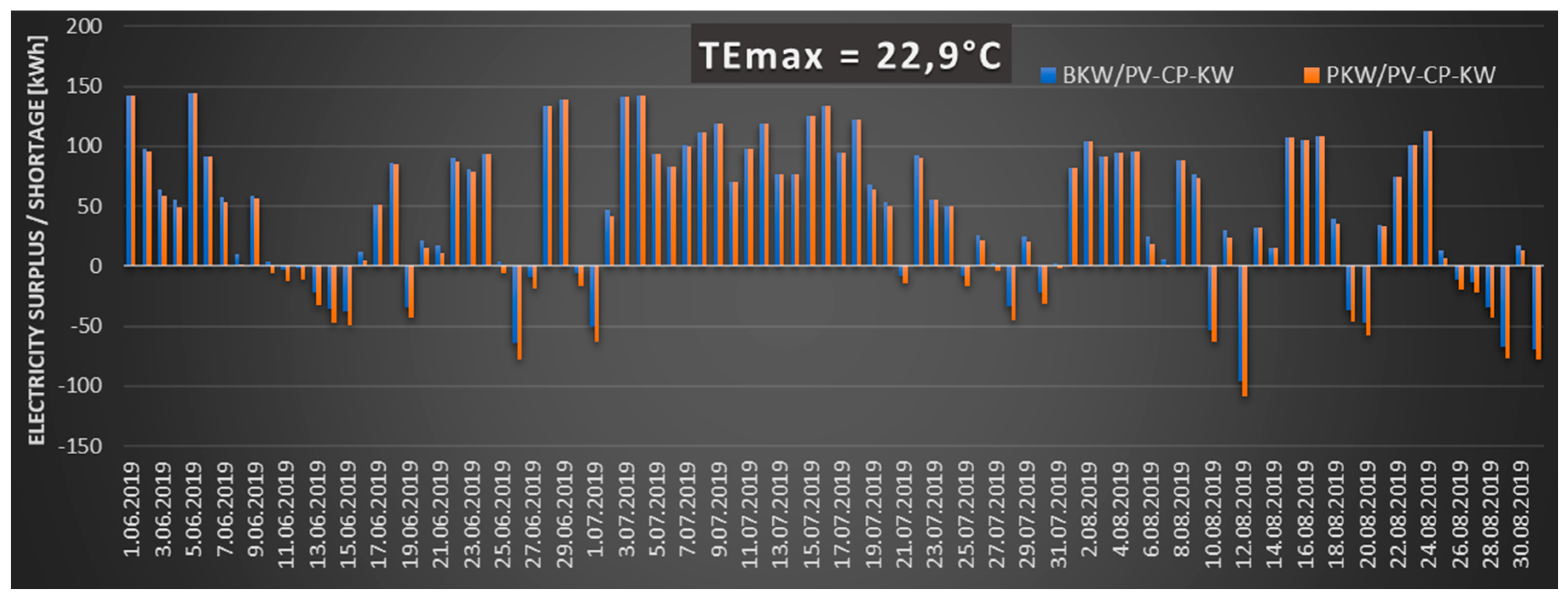
Figure 8.
Excess and daily shortage of electricity produced from the existing PV installation in the case of the upper limit of thermal comfort TEmax = 24°C.
Figure 8.
Excess and daily shortage of electricity produced from the existing PV installation in the case of the upper limit of thermal comfort TEmax = 24°C.
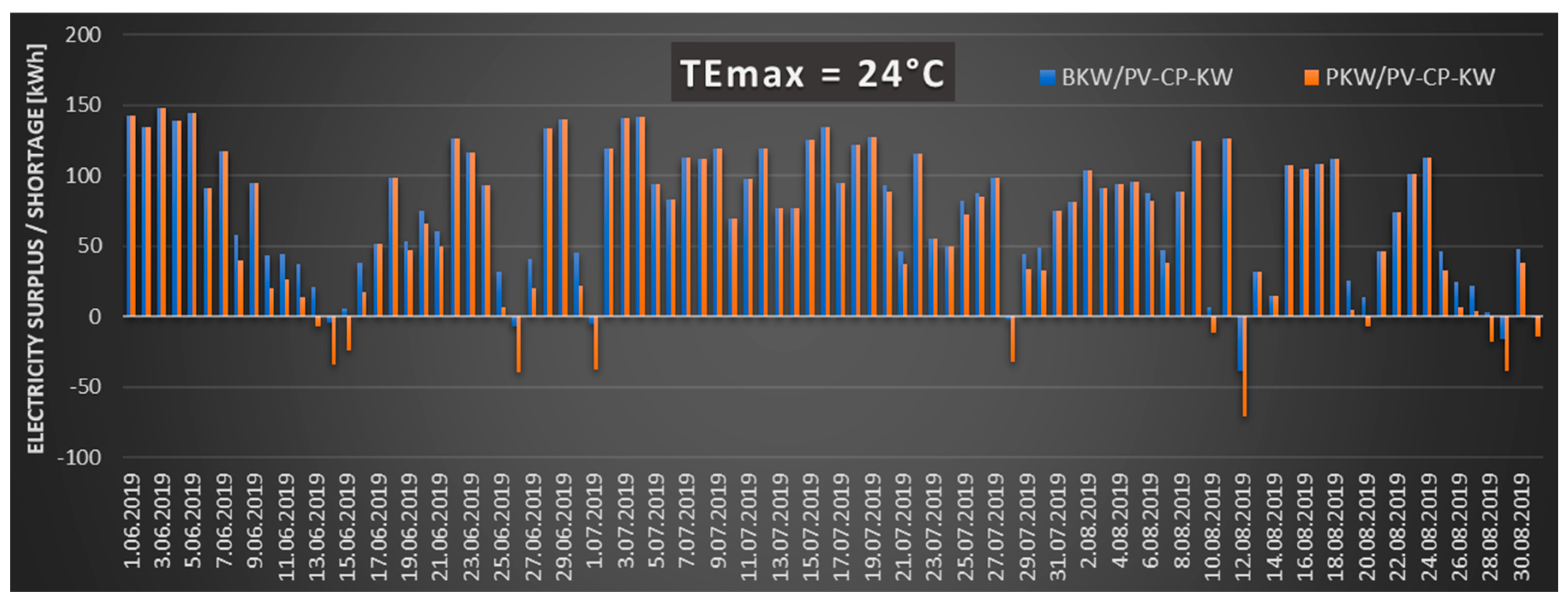
Figure 9.
Excess and daily shortage of electricity produced from the existing PV installation in the case of the upper limit of thermal comfort TEmax = 25°C.
Figure 9.
Excess and daily shortage of electricity produced from the existing PV installation in the case of the upper limit of thermal comfort TEmax = 25°C.
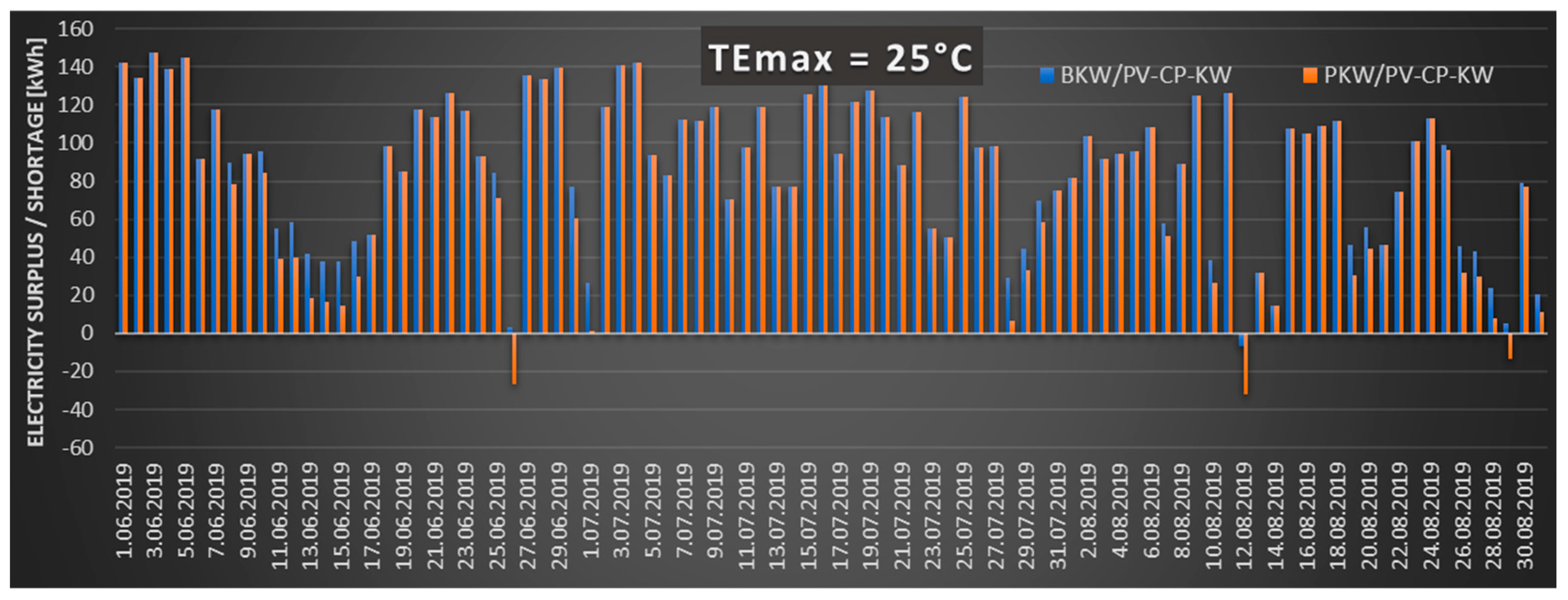
Figure 10.
The value of the EP, EK and EU indicators for the individual variants and the different assumptions of the upper limit of thermal comfort of TEmax.
Figure 10.
The value of the EP, EK and EU indicators for the individual variants and the different assumptions of the upper limit of thermal comfort of TEmax.
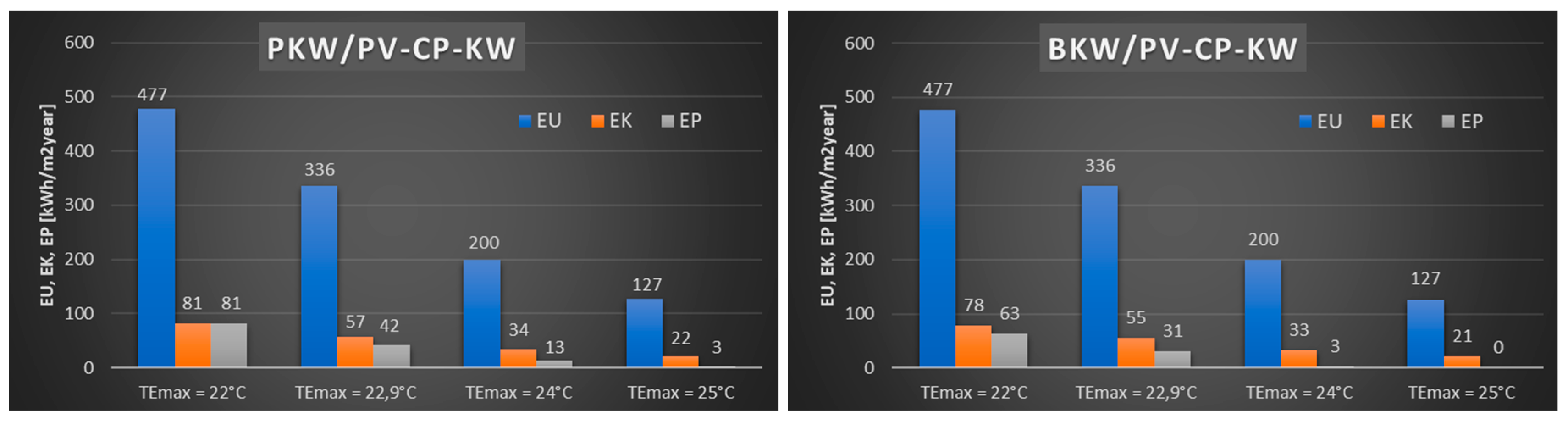
Figure 11.
Comparison of Eco-indicators of individual impact categories for the analyzed variants.
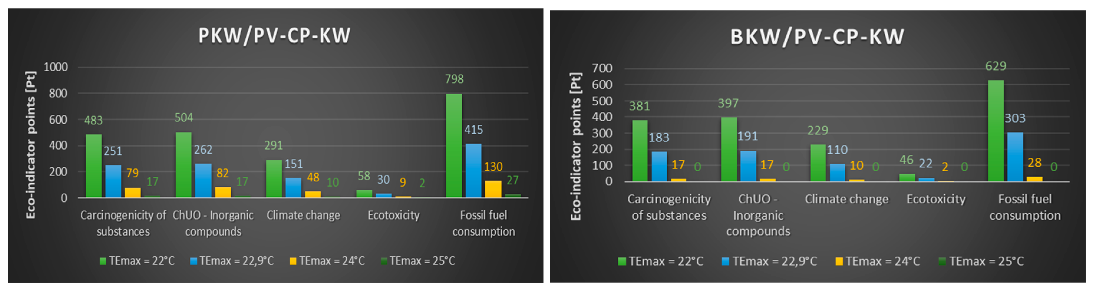
Figure 12.
Comparison of Eco-indicators of individual categories of damage for the analysed variants.
Figure 12.
Comparison of Eco-indicators of individual categories of damage for the analysed variants.
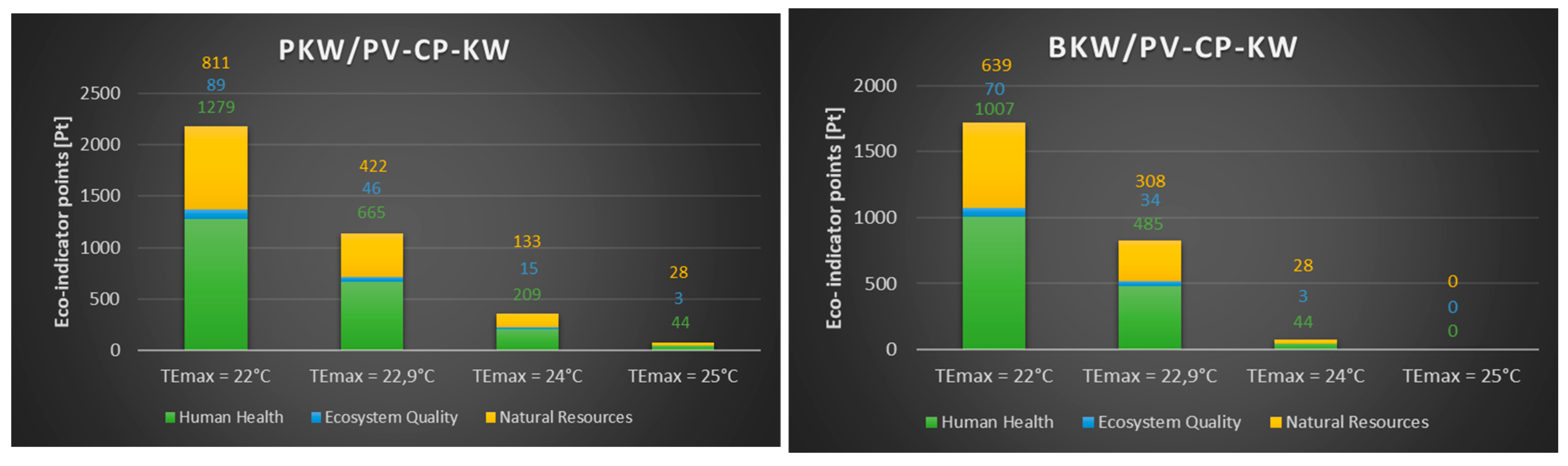
Figure 13.
The LLC indicator's value for varying upper limits of thermal comfort (TEmax) is examined for two cooling system variants.
Figure 13.
The LLC indicator's value for varying upper limits of thermal comfort (TEmax) is examined for two cooling system variants.
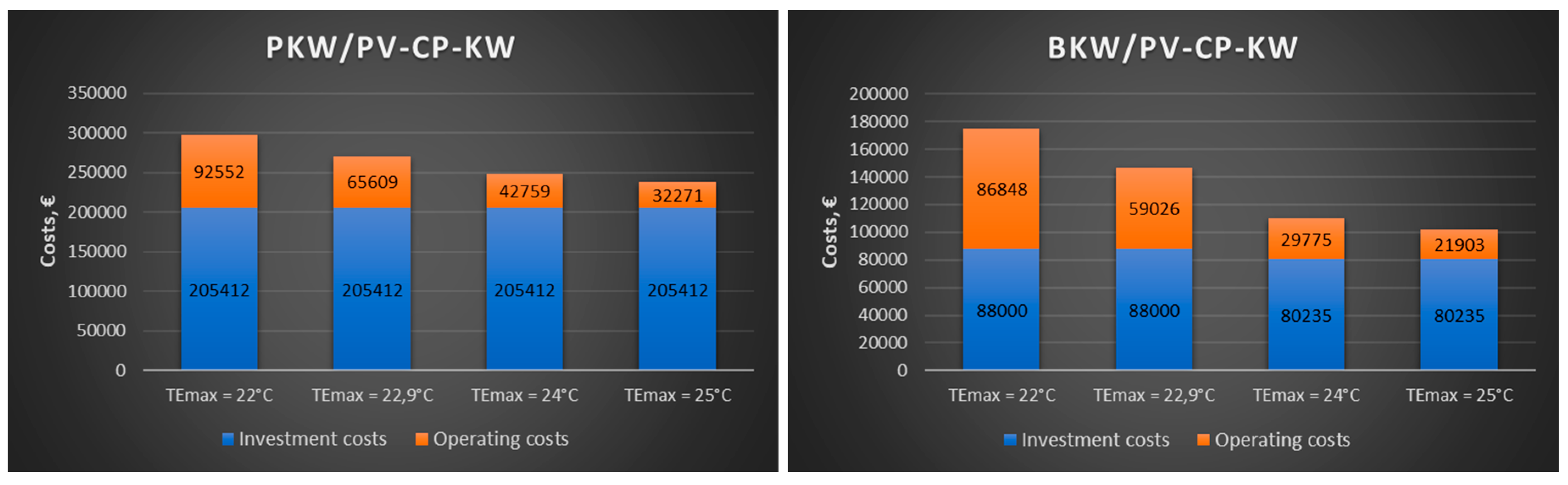

Table 1.
A comparative analysis of basic adiabatic cooling systems [26,27,28,29,30,31,32,33,34,35,36,37,38].
| Adiabatic cooling type | Mechanism of action | Cooling efficiency | Advantages | Constraints |
| Direct Evaporative Cooling (DEC) | Direct air humidification via cooling inserts | 60-95% in dry conditions | Simple design, low investment and operating costs | Increases air humidity, risk of microorganism growth |
| Indirect Evaporative Cooling (IEC) | Heat exchanger separates moist air from cooled air | 40-70% in humid conditions | Cools without increasing humidity | Heat exchanger complexity, higher cost |
| Indirect–Direct Hybrid (IDEC) | IEC + DEC connection in a cascade system | 70-110% (relative to DEC efficiency alone) | Very high efficiency, RH control | Higher investment cost, higher service complexity |
| Misting / Water Spray Systems | Spraying fine water droplets in the user area | Local T reduction of 2-7 °C | Effective subjective cooling, low barrier to deployment | Increases local humidity, requires water filtration, sanitary risks |
| Regenerative IEC (R-IEC) | Regenerative heat exchangers in duct systems | SEER: 10-16 (experimental) | Very high seasonal efficiency | High investment cost, the need to control water quality |
Table 2.
Basic data of the test object [25].
Table 2.
Basic data of the test object [25].
| Element | Symbol | Unit | Value |
| length x width x height | L x S x H | m | 36 x 4 x 2 |
| surface | A | m2 | 144 |
| volume | V | m3 | 288 |
| number of photovoltaic modules | N | - | 104 |
| dimensions of photovoltaic modules | - | m | 2.135 x 0.975 |
| unit power of photovoltaic modules | Pj | W | 275 |
| number of people in reference area | No | - | 126 |
Table 3.
Technical parameters of the devices adopted in the analyzed variants of the cooling system.
Table 3.
Technical parameters of the devices adopted in the analyzed variants of the cooling system.
| Device | Technical data |
| PV module | power: 275 Wp. |
| indirect evaporative air conditioner (central unit) | air flow: 23 040 m3/h nominal cooling capacity: 160 kW, water consumption: 423 l/h,electricity consumption: 11,8 kW. |
| indirect evaporative air conditioners (local units) | nominal cooling capacity: 18,4 kW, water consumption: 70 l/h,electricity consumption: 13,5 kW. |
Table 4.
Results of calculations of constant heat gains QZC-S, for the research object [25].
Table 4.
Results of calculations of constant heat gains QZC-S, for the research object [25].
| Type of constant heat gain | Symbol | Unit | Value |
| Heat gains from people for the reference area | QL | kW | 22 |
| Profits from running motor engines of vehicles located directly at the reference area | QP | kW | 72 |
| Constant heat gains | QZC-S | kW | 94 |
Table 5.
The following study will compare the coefficients that have been adopted for the calculation of the energy effect. [54].
Table 5.
The following study will compare the coefficients that have been adopted for the calculation of the energy effect. [54].
| Symbol of the variant | SEER ref [-] |
Ci [-] | ηC,s [-] | ηC,d [-] | ηC,e [-] |
wc [-] | w el [-] |
|---|---|---|---|---|---|---|---|
| PKW/PV-CP-KW | 13,56 | 0,5 | 1 | 0,9 | 0,96 | 0 | 0 / 2,5 |
| BKW/PV-CP-KW | 12,27 | 0,5 | 1 | 1 | 1 | 0 | 0 |
Table 6.
The coefficients used in the calculation of the Eco-indicators of the impact category and the category of damage.
Table 6.
The coefficients used in the calculation of the Eco-indicators of the impact category and the category of damage.
| Impact category - Eco-indicator, EkW, Pt/GJ | Damage category - Eco-indicator, EkW, Pt/GJ | |||||
| Electricity - SEN | Electricity - SEN | |||||
| Carcinogenicity of the substance | 49,445 | Human health | 130,806 | |||
| PDO - Organic compounds | 0,014 | |||||
| PDO - Inorganic compounds | 51,524 | |||||
| Climate change | 29,738 | |||||
| Ionizing radiation | 0,039 | |||||
| Ozone depletion | 0,045 | |||||
| Ecotoxicity | 5,938 | Ecosystem quality | 9,090 | |||
| Acidification | 1,981 | |||||
| Land use | 1,171 | |||||
| Mineral consumption | 1,365 | Natural resources | 83,001 | |||
| Fossil fuel consumption | 81,636 | |||||
| Amount | 222,897 | Amount | 222,897 | |||
Table 7.
Summary of assumptions used for the calculation of the economic effect.
| Element | TEmax = 22°C | TEmax = 22,9°C | TE max = 24°C | TEmax = 25°C |
| QCH [kWh year-1] | 68688 | 48412 | 28803 | 18221 |
| n [h] | 667 | 474 | 286 | 183 |
| A [m2] | 144 | |||
| Θ [year] | 25 | |||
| s [%] | 5 | |||
Table 8.
Summary of assumptions used for the calculation of the economic effect.
| Symbol of the variant | Price of energy carriers | |
| Electricity | Water/ Sewage | |
| [EUR/kWh] | [EUR/m3] | |
| PKW/PV-CP-KW | 0,27 | 3,53 |
| BKW/PV-CP-KW | ||
Disclaimer/Publisher’s Note: The statements, opinions and data contained in all publications are solely those of the individual author(s) and contributor(s) and not of MDPI and/or the editor(s). MDPI and/or the editor(s) disclaim responsibility for any injury to people or property resulting from any ideas, methods, instructions or products referred to in the content. |
© 2025 by the authors. Licensee MDPI, Basel, Switzerland. This article is an open access article distributed under the terms and conditions of the Creative Commons Attribution (CC BY) license (http://creativecommons.org/licenses/by/4.0/).
Copyright: This open access article is published under a Creative Commons CC BY 4.0 license, which permit the free download, distribution, and reuse, provided that the author and preprint are cited in any reuse.


