
Submitted:
26 September 2025
Posted:
10 October 2025
You are already at the latest version
Abstract
With the increasing frequency and intensity of extreme weather events, there is a growing need to develop innovative and accessible methods for environmental monitoring. This work presents a solution based on natural trees equipped with a low-cost embedded system. The innovative idea is that measuring only internal temperature of a tree around its trunk, it is possible to evaluate some weather parameters, such as wind speed and direction. To evaluate this relationship, a multiscale decomposition technique (Discrete Wavelet Transform) and machine learning models (Random Forest, Gradient Boosting, SVM, and Linear Regression) were applied. Among the models tested, Random Forest achieved the best results, demonstrating high accuracy with an error of 6.60%. As an important outcome, the result shows that the proposed tree-based solution is viable for weather monitoring in hard-to-reach places, particularly in the context of forest fire prevention.
Keywords:
wind forecasting
; wavelet transform
; machine learning
; climate modeling
; temperature sensors
; trees
1. Introduction
In recent years, the US, Canada, Brazil, and other countries have faced a significant increase in the occurrence of forest fires, highlighting the need for new technologies for monitoring and control. These events are triggered by a combination of natural and human factors, such as prolonged droughts, rising average temperatures, and illegal burnings, and are further aggravated by the intensification of global climate change [1].
To better understand the behavior of forest fires, it is necessary to evaluate the environ- mental parameters that influence them. One of them is the wind, which is a primary cause of flame propagation in an unforeseen manner, as wind intensity and direction directly influence fire spread, and the ignition of new fire outbreaks over long distances [2]. In this context, these conditions present complex challenges for controlling and combating forest fires, demanding the development of more accurate predictive tools adapted to forest environments.
Considering the critical role of wind in fire propagation, forecasting its direction and intensity in real time, especially in areas with dense vegetation and difficult terrain, remains a complex task. Some wind forecasting models, such as in [3], incorporate topographic factors such as terrain and vegetation cover to estimate wind speed at flame height. Other studies, such as in [4], emphasize the critical role of extreme atmospheric conditions, especially the combination of prolonged drought and intense winds, during large-scale fire events.
In this context, this work proposes an innovative alternative to the use of conventional weather stations: the use of living trees equipped with temperature sensors installed at different heights, cardinal orientations, and trunk depths. The central hypothesis is that the internal thermal variations captured by these sensors indirectly reflect external weather patterns, such as wind direction and speed. The objective of this work is to introduce the concept of a natural weather station.
(NWS) based on trees and mainly to assess the potential of internal temperature level measurement in tree trunk, combined with mathematical modeling techniques, as a complementary tool for real-time weather monitoring, focusing on low-cost, low-energy consumption solutions, particularly in regions with limited meteorological infrastructure.
2. Related Work
Forest fire monitoring has become increasingly sophisticated, driven by advances in remote sensing technologies, artificial intelligence, and predictive modeling. The use of satellite imagery, drone-mounted sensors, and automated detection systems has signif- icantly enhanced the ability to prevent, detect, and respond to wildfires across various regions of the world.
Among the most widely used technologies are optical and thermal sensors mounted on satellites such as Sentinel-2, Landsat, and MODIS [5]. These sensors allow large-scale monitoring with spatial and temporal resolution sufficient to identify active heat sources and vegetation changes. Automatic detection models based on deep learning, such as convolutional neural networks and hybrid architectures, have been successfully applied to identify fires from multispectral images, achieving accuracy rates above 80 percent [6].
In addition to these orbital platforms, unmanned aerial vehicles (UAVs) have gained prominence in monitoring hard-to-access areas. Drones equipped with RGB, multispectral, and hyperspectral cameras enable detailed real-time analysis of vegetation, soil, and fire spread. These tools have already been successfully used in various environmental monitoring applications, including agricultural pest control, and are now being adapted for forest fire contexts [7]. Another important advancement is the use of thermal images generated by infrared sensors to automatically locate active fire perimeters. Edge detection systems based on the Canny algorithm have proven capable of accurately mapping burned areas and tracking their progression over time, producing cartographic outputs compatible with GIS platforms such as QGIS and Google Earth [8].
Fire spread forecasting is also a rapidly advancing field. Models such as WRF-SFIRE (Weather Research and Forecasting model coupled with the SFIRE module) combine at- mospheric variables and ground data to simulate fire behavior in real time. WRF-SFIRE is an extension of the widely used WRF weather model, enhanced with the SFIRE module, which incorporates physical equations to simulate fire dynamics based on topography, vegetation type, and real-time meteorological conditions.
These models rely on information such as wind speed, air humidity, vegetation type, and fuel load, which can be derived from geospatial data and satellite images. In a recent application in the Himalayas, the system was able to predict the burned area with strong correlation to satellite-based observations, demonstrating the operational feasibility of these tools for supporting firefighting agencies [9].
Finally, the book Fundamentals of Satellite Remote Sensing emphasizes the importance of integrating remote sensing data with Geographic Information Systems (GIS), highlight- ing the relevance of radar data and near-surface sensors such as UAVs for large-scale environmental monitoring [10].
3. Experimental Setup
To implement the proposition of predicting wind speed and direction based on internal temperature levels of a tree, it was necessary to set up an experimental arrangement for accurate and reliable data acquisition. This setup consists of two main pieces of equipment: a tree equipped with temperature sensors (the proposed tree-based Natural Weather Station, NWS) and an automatic weather station located near the tree. The automatic weather station serves as a reference, and its data are used for comparison between the internal temperature conditions of the tree and the external environmental conditions, such as wind speed and direction. In summary, while the NWS records internal trunk temperatures at different points, the weather station records surrounding weather parameters.
The following sections provide more detailed information about each of these systems, explaining how they were installed, how they operate, and how they contribute to the results obtained in this study.
3.1. The Proposed Natural Weather Station
The proposed tree-based NWS is a living tree equipped with temperature sensors, a microcontroller, and a wireless radio. The sensors were installed directly in the tree trunk at different depths, heights, and cardinal directions (North, South, East, West), aiming to monitor the internal thermal dynamics in response to external environmental variations, such as solar radiation, shading, and wind effects. The tree-based NWS was deployed at the campus of the Federal University of Paraíba, Brazil, as shown in Figure 1.
The temperature sensor used is the DS18B20, selected for its precision, low power consumption, and ease of field installation. These sensors operate using a digital protocol; instead of transmitting analog signals, they directly send temperature data in digital format, which reduces interference and simplifies data reading [11].
One of the main advantages of the DS18B20 is the use of the 1-Wire bus, which allows multiple sensors to be connected through a single data wire. This simplifies the physical setup, as there is no need for multiple cables. Each sensor has a unique digital address, allowing individual identification even when connected in parallel [12].
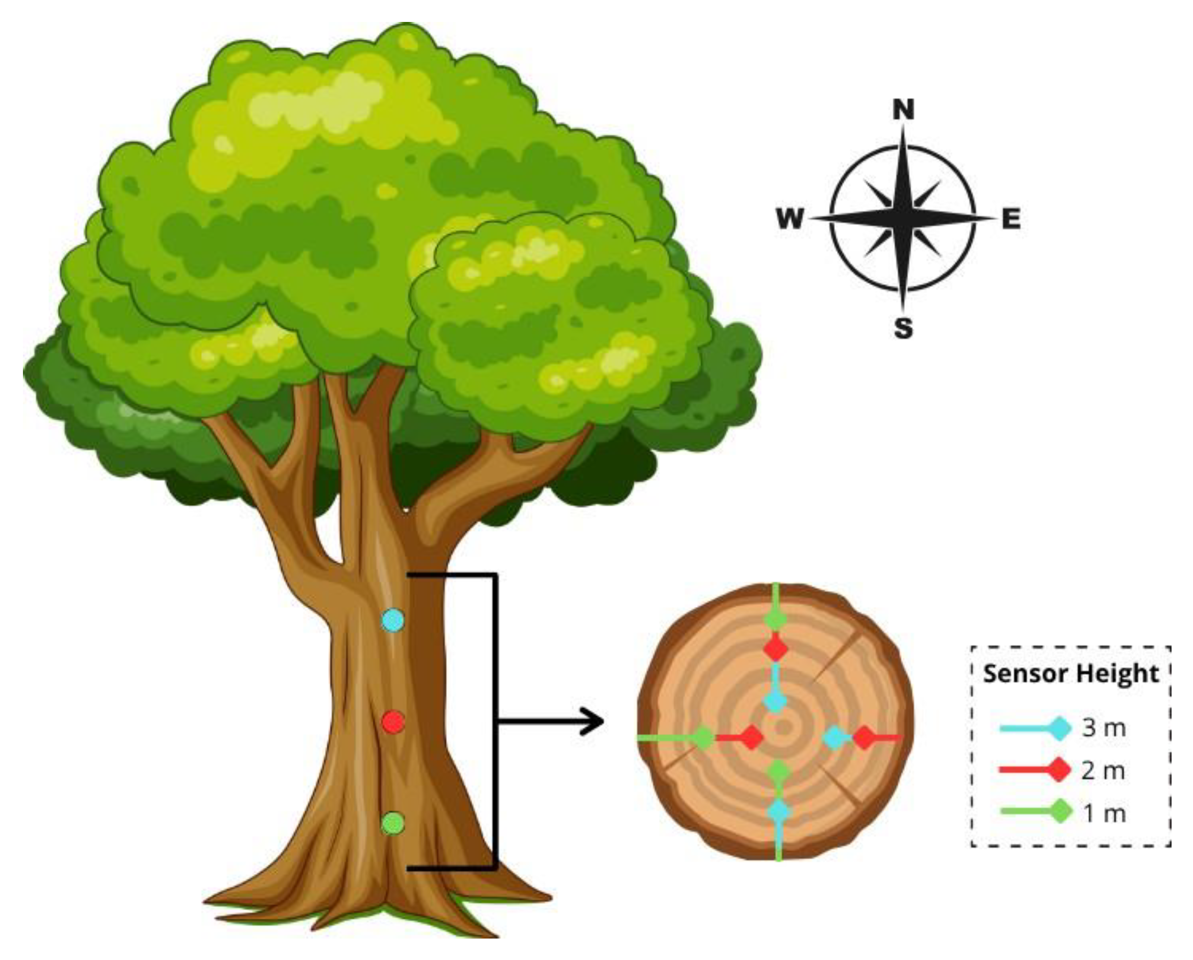
In the tree-based NWS, the sensors were grouped by height: 1 m, 2 m, and 3 m above the ground. At each height, they were installed in different directions (North, South, East, and West) and at various depths inside the trunk, ranging from 4.0 cm to 13.5 cm. This configuration makes it possible to capture thermal variations at different points in the tree, both vertically and horizontally.
Figure 3 visually illustrates the distribution of the sensors, and Table 1 summarizes all the positions adopted in the experiment.
Figure 2.
1-Wire buses interconnecting arrays of DS18B20 temperature sensors.
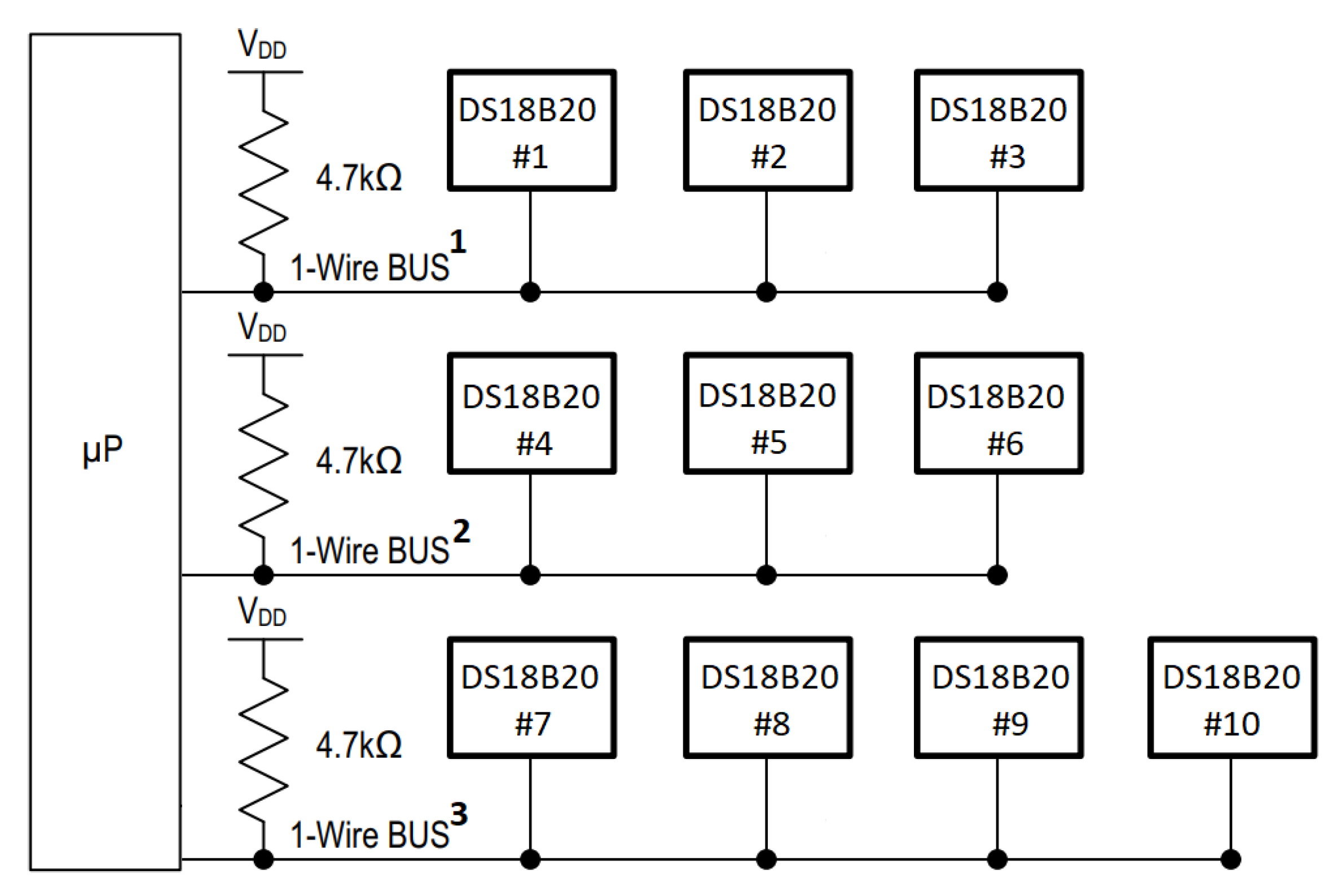
Figure 3.
Sensor distribution around the tree trunk.
Temperature values were recorded continuously throughout the whole duration of the experiment. Figure 4 presents some of the time series obtained, highlighting thermal variations at different depths, heights, and orientations of the trunk. It can be observed, for instance, that although the sensors are positioned close to each other and follow similar patterns, their thermal responses vary according to depth and exposure as well as the external weather conditions.
The DS18B20 temperature sensors were connected in arrays of three sensors, totaling three 1-Wire buses: 1-Wire Bus 1, 1-Wire Bus 2, and 1-Wire Bus 3, as shown in Figure 2. 1-Wire Bus 1 connected the set of sensors at 1 m height, 1-Wire Bus 2 the sensors at 2 m, and 1-Wire Bus 3 the sensors at 3 m. On 1-Wire Bus 3, an additional sensor measured the external temperature. Up to four sensors were attached per 1-Wire bus due to the drive capability limitation of the microcontroller I/O pin.
The microcontroller used in the system is ARM Cortex-M0-based, embedded on a commercial board (Adafruit Feather) integrated with a 915 MHz LoRa radio module. With this setup, it is possible to read the sensors, process the data, and transmit packets containing temperature readings. The embedded system is powered by a solar panel, a battery, and a battery management system (BMS), which ensures energy autonomy even in areas without direct access to electricity. This reinforces the sustainability approach and enables continuous data collection throughout the entire monitoring period, including in hard-to-reach forest environments.
Data transmission to a cloud-based storage system is carried out using LoRa technology, which allows long-range wireless communication with low energy consumption. The packets sent by the system are received by a LoRa gateway, approximately 500 m away, which works as a bridge to the Internet. The gateway forwards the data to the storage system, where they are preprocessed and used to build models to forecast weather variables.
The complete architecture for measuring tree trunk temperatures and sending them to the cloud is shown in Figure 5. It enables continuous, reliable, and high-resolution monitoring of the tree’s internal temperature.
3.2. Weather Station
To obtain environmental data, the automatic weather station installed at the Center for Alternative and Renewable Energies (CEAR) of the Federal University of Paraíba (UFPB), Brazil, was used. The weather station is located approximately 290 m from the proposed tree-based NWS, ensuring sufficient proximity to accurately represent the atmospheric conditions affecting the monitored tree. Among the various instruments present in the automatic weather station, two of them stand out as fundamental to this study: the anemometer, responsible for measuring wind speed, and the wind vane, which records wind direction, as shown in Figure 6. The data acquired from the automatic weather station are stored in a data logger and in an online storage service. These data have been used as the reference variables to assess the accuracy of the predictions generated by the models based on the tree’s thermal time series.
Figure 7 shows the time series of wind direction (upper graph) and wind speed (lower graph) recorded by the CEAR/UFPB weather station during a period of data collection. Daily wind-intensity patterns can be observed, usually occurring during the hottest hours of the day, as well as significant variations in wind direction. These data are essential for evaluating the impact of wind on the thermal dynamics of the tree.
In addition to measuring wind, the station also collects other weather variables, such as air temperature and humidity, through a thermo-hygrometer, which expands its potential for applications in future studies.
The weather station operates autonomously, powered by a solar panel, and performs continuous data logging through a data logger that stores the data and, when necessary, transmits them online for remote visualization or integration with other systems. This setup enables the acquisition of reliable and up-to-date time series, which are essential for forecasting the desired variables—wind speed and direction.
4. Data Processing and Models Used
To ensure the proper training of the forecasting models for applying to the tree-based NWS, it was necessary to set up a preliminary data processing stage. This stage included organizing, preparing, and applying the necessary transformations to the collected data. At this point, the measurements taken by the tree-based NWS and the weather station were synchronized and prepared for analysis. Although this study relies on ground- based sensors, the thermal time series collected could potentially be used to calibrate or validate remote sensing data from satellite sources, enhancing multi-source environmental monitoring efforts.
In addition, mathematical techniques were applied to extract important features from the obtained temperature series based on the Discrete Wavelet Transform (DWT), which allows the decomposition of the series into different time scales. This reveals both long-term trends and rapid local fluctuations, which are necessary to capture patterns associated with the wind.
The following sections present the steps taken for data processing, as well as the machine learning models used to predict wind speed and direction. The objective is to demonstrate how the raw data were processed and transformed into suitable inputs for the models.
Figure 8 provides a visual summary of the methodology adopted, from data acquisition to final modeling.
4.1. Data Collection and Processing
The data used in this work were obtained from the tree-based NWS deployed in a tree located at the Center for Alternative and Renewable Energies (CEAR/UFPB). The temperature sensors of the tree-based NWS recorded temperatures every 10 minutes over a continuous period of 47 days, capturing thermal variations associated with day and night cycles.
External weather data were collected simultaneously—specifically wind speed and direction—through the automatic weather station located near the monitored tree. The wind data were temporally synchronized with the tree’s thermal measurements, ensuring that the analyses were based on time-aligned series.
After collection, the raw data were organized into a database containing tree tem- perature data, timestamps, and corresponding wind data. The first processing step was temporal standardization, ensuring that the timestamps were correctly distributed and that there were no gaps in the sequence of records.
The temperature readings from the sensors were defined as explanatory (input) vari- ables, while wind speed and direction were established as target (output) variables in the forecasting models. To handle any missing values, a simple local averaging technique was used, replacing missing entries with the average of nearby values for that variable, in order to maintain the statistical consistency of the series.
As a final step in the preprocessing, all temperature values were normalized; that is, they were transformed to be on a common scale—typically ranging from 0 to 1 or adjusted to have a mean of 0 and a standard deviation of 1. This process prevents sensors with higher absolute values from having a disproportionate influence on the model’s learning.
For example, if one sensor records temperature between 28◦C and 32◦C, and another between 20◦C and 22◦C, the first sensor would naturally have larger numerical values. Without normalization, the model might prioritize this sensor simply because of its scale, not because it provides more useful information. Normalization adjusts both sensors’ readings so that each contributes equally to the learning process, regardless of their original value ranges.
In addition to the original thermal variables, new variables were created, called Temp Gradients, which represent the thermal gradient—that is, the difference between the temperatures recorded at different positions on the trunk. This variable aims to highlight thermal variations associated with external disturbances, such as changes in wind flow around the tree, thus providing additional information for the predictive models.
4.2. Discrete Wavelet Transform
Environmental time series, such as temperature variations measured over time, often exhibit behaviors that change constantly, with periods of stability and moments of rapid variation. Therefore, it is important to use methods capable of analyzing these changes at different time scales. One such method is the Discrete Wavelet Transform (DWT) [13].
In this study, the DWT was used to transform the temperature data collected from the tree trunk into sets of information that reveal both slower trends and faster variations in the signal. For this purpose, a wavelet of the Daubechies family of order 4 (db4) was used, which is known for its efficiency in detecting subtle changes in data [14].
The DWT divides each temperature series into two main types of information:
- Approximation coefficients (cA): represent the overall behavior of temperature over time, such as trends and averages; and
- Detail coefficients (cD): highlight faster and more abrupt variations, such as peaks and sudden fluctuations.
In the end, each time series was decomposed into four levels of detail, resulting in one set of cA and four sets of cD, as shown in Figure 9. This means that the same signal can be observed at different resolutions, as if using magnifying glasses with varying degrees of zoom.
After this transformation, a correlation analysis was performed between the resulting coefficients and the wind data (speed and direction). This helped identify which parts of the temperature signal were most related to meteorological phenomena.
The coefficients that showed the strongest relationship with wind behavior were then selected as input variables for the forecasting models used in this work. In this way, the DWT helped convert raw data into meaningful features for training the machine learning algorithms.
4.3. Models Developed
After extracting thermal features using the Discrete Wavelet Transform (DWT), predic- tive models were developed to estimate wind speed and direction based on the temperature time series. Four algorithms were evaluated: Random Forest, Gradient Boosting, Support Vector Machines, and Linear Regression.
The data were split into 80% for training and 20% for testing, ensuring independence between the datasets. To prevent the models from simply memorizing the training data, a phenomenon known as overfitting, the hyperparameters were automatically optimized using the GridSearchCV technique with cross-validation. This optimization was particu- larly important for the Random Forest (RF), Gradient Boosting (GB), and Support Vector Machines (SVM) models, as they tend to be more sensitive to parameter configuration [15]. The following sections describe the models used and their configurations:
Random Forest (RF)
The first model evaluated was Random Forest, a technique that builds multiple de- cision trees using subsets of the training data and available variables, as illustrated in Figure 10. Each tree produces a prediction, and the final result is obtained by averaging these individual outputs, as is typical in regression tasks [16]. This process, known as bagging, reduces model variance and improves robustness.
In the context of this work, Random Forest proved a suitable solution due to its ability to handle nonlinear data, tolerate noise, and provide insights into which variables most influence the predictions. Initially, the model was tested with default settings and later fine-tuned using GridSearchCV to determine the optimal number of trees, maximum tree depth, and the minimum sample size required for each split.
Gradient Boosting (GB)
Gradient Boosting also relies on decision trees, but it uses a sequential approach.
Instead of creating independent trees, the model builds each new tree to correct the errors of the previous one, using the gradient of the loss function as a guide [17], as shown in Figure 11. This cumulative learning process tends to produce highly accurate models, but it is also more sensitive to the choice of hyperparameters.
Combinations with different numbers of trees, tree depths, and learning rates were tested, aiming to minimize cumulative error without compromising the model’s ability to generalize. Gradient Boosting is particularly useful for identifying complex patterns, but it requires greater attention to avoid overfitting to the training data.
Support Vector Machines (SVM)
When adapted for regression tasks, the SVM model is known as Support Vector Regression (SVR). It seeks to find a hyperplane that keeps most of the data within an acceptable error margin (ϵ), penalizing the points that fall outside this range. The model is illustrated in Figure 12. The degree of penalization is controlled by the regularization parameter (C) [18].
An important feature of SVR is the use of kernel functions, which transform the data to allow the fitting of nonlinear patterns. In this study, two types of kernels were tested: linear and radial basis function (RBF), the latter being capable of capturing curved patterns. 291 Despite its flexibility, the model requires careful tuning of parameters and has a higher 292 computational cost. To address these limitations, its application was accompanied by 293 systematic hyperparameter optimization.
Linear Regression (LR)
As a baseline for comparison, Linear Regression (LR) was used. This is a simple statis- tical model that assumes a linear relationship between the input variables (temperature) and the output variables (wind speed and direction) [19]. Its main advantage is ease of interpretation. However, because it does not capture nonlinear relationships or abrupt variations, which are common in environmental data, it tends to show lower predictive performance, higher residual errors, and limited adaptability to interactions between vari- ables. Even so, its inclusion in the study was important to quantify the performance gain achieved with more sophisticated models.
Model evaluation was based on three main metrics: mean squared error (MSE), which quantifies the average magnitude of the errors; the coefficient of determination (R2), which measures how well the model explains the variability in the data; and the mean absolute 306 percentage error (MAPE), which expresses the relative prediction accuracy in percentage 307 terms. All models were tested separately for predicting wind speed and direction, always 308 using the same input structure to ensure fair comparisons.
5. Results
After data preprocessing and the development of predictive models, it was possible to analyze the results obtained at each stage of the research. This section presents the main findings of this work, starting with the analysis of the coefficients extracted using the Discrete Wavelet Transform (DWT), followed by the predictions made for wind speed and direction.
The goal is to demonstrate how the internal temperature variations recorded by the tree-based NWS can serve as a basis for estimating wind patterns in the external environ- ment. To this end, comparative graphs, tables with model results, and interpretations are presented to help understand the system’s behavior.
5.1. Discrete Wavelet Transform Coefficients
The application of the DWT to the temperature series allowed the extraction of ap- proximation coefficients (cA), which capture smoother and more persistent patterns, and detail coefficients (cD), which reflect rapid and localized variations.
The level 0 approximation coefficients (cA) showed consistent behavior across sen- sors, even when installed in different positions along the trunk. For example, sensor T1N13 ranged between 107.208 and 107.251, while T3N4 recorded values between 104.956 and 105.100. These values represent the overall trend or average behavior of the temperature signal after filtering out short-term fluctuations, similar to how a moving average captures the general direction of a time series.
The important point is not the exact numerical values, but the similarity in their range across different sensors, indicating that the trunk exhibits a stable thermal profile over time, with common patterns shared along its structure. Figure 13 illustrates this coherence, highlighting the similarity in the approximation coefficient patterns over time.
On the other hand, the detail coefficients (cD), especially at the first level (cD1), showed greater dispersion among the sensors. This is consistent with their role in capturing rapid thermal fluctuations, which are more sensitive to influences such as solar radiation, shading, and momentary environmental variations. At deeper decomposition levels, such as cD3 and cD4, variability was reduced, indicating a natural smoothing of the signals at broader temporal scales.
To assess the explanatory potential of these coefficients, a Pearson correlation analysis was performed between them and the two target meteorological variables, wind speed and direction. The cA coefficients showed the highest correlations, mainly with wind direction, with values ranging from 0.4 to 0.5. In contrast, the correlations with wind speed were lower, ranging from 0.1 to 0.2. The correlation results are presented in Table 2.
Based on these results, it was decided to use only the level 0 approximation coefficients in the predictive modeling. This decision was supported both by the observed stability among the sensors and by the greater statistical relevance of the cA coefficients, which more effectively capture dominant trends in the time series. Although the detail coefficients were not directly used in the models, they provide a complementary view of short-term thermal variations and may be useful in future analyses.
5.2. Wind Speed Forecast
The machine learning models were applied to predict wind speed, using as input the approximation coefficients extracted from the temperature time series. Table 3 presents the results obtained for the evaluation metrics (MSE, R2, and MAPE).
The optimized Random Forest (RF) model showed the best performance, with the low- est errors and the highest explanatory capacity. This is consistent with the findings of [20], who identified RF as one of the most robust algorithms for wind prediction, highlighting its stability when applied to nonlinear environmental data. Even the RF model without hyperparameter tuning demonstrated good generalization ability.
Gradient Boosting, although showing competitive performance, was more sensitive to abrupt variations in the time series, which affected its predictive stability. This behavior is similar to that observed by [21], who emphasized the need for more careful tuning for GB to perform well in highly variable environments.
SVM, even with optimization, achieved intermediate performance, showing a ten- dency to smooth out peaks and valleys. This limits its response in cases of extreme events, reflecting the limitations discussed by [22] regarding the difficulty of SVM in handling multiple correlated variables and inconsistent patterns.
Finally, Linear Regression was the worst-performing model, with a MAPE above 38% and an R2 below 0.6, highlighting its limitations when faced with the complexity and nonlinearity of the time series. This confirms conclusions in the literature, such as [21], which point out the inadequacy of linear models for meteorological forecasting.
Figure 14 provides a visual comparison between the actual values and the predicted wind speed, reinforcing the results observed in the quantitative metrics.
In addition to model selection, it is important to emphasize that data quality also positively influenced the results. The strategic placement of sensors in the tree made it possible to capture both vertical and horizontal thermal gradients, which proved to be relevant for the prediction task. This approach is in line with the findings of [23], who advocate the use of derived physical variables as a key factor in the performance of predictive models.
5.4. Wind Direction Forecast
The prediction of wind direction followed the same approach used for wind speed, using the approximation coefficients obtained through the DWT as input. Table 4 presents the performance results of the models, once again considering the evaluation metrics MSE, R2, and MAPE.
The optimized RF model once again stood out, achieving the best overall performance 385 (MSE of 176.13, R2 of 0.867, and MAPE of 6.60%). Its strong performance reinforces its 386 robustness in dealing with seasonal patterns and the periodic nature of the wind direction 387 variable. The ability of RF to handle nonlinear structures and noisy data makes it more 388 suitable for forecasting tasks, as previously highlighted by [20].
Gradient Boosting again showed competitive performance compared to RF, although slightly inferior, demonstrating greater sensitivity to noise in the data, as observed by [21]. SVM, on the other hand, had difficulty capturing rapid changes in wind direction, even with fine-tuned kernel settings. This confirms the observations made by [22] regarding its limitations in dynamic and complex environments.
Linear Regression once again recorded the worst performance, with an R2 below 0.5 and MAPE above 14%. This poor fit confirms the limitations of linear models when dealing with meteorological contexts that exhibit cyclical and nonlinear behavior.
Figure 15 presents the graphical comparison between actual and predicted wind direct.
Together with the results for wind speed, the data confirm that the optimized RF was the most efficient model for both target variables. The multiscale feature extraction using the DWT and the use of the thermal gradient as an auxiliary variable further enhanced its predictive capacity, validating the approach proposed in this study for applications in low-cost and high-accuracy environmental monitoring.
6. Conclusions
This work investigated the potential of thermal data collected from sensors installed in a tree for predicting wind direction and speed. The methodology combined distributed temperature sensors at different trunk depths, heights, and directions with the application of the Discrete Wavelet Transform (DWT), aiming to capture thermal variations at multiple temporal scales. This approach enabled the transformation of the tree’s internal thermal behavior into a sensitive indicator of external atmospheric changes.
The analysis demonstrated that the approximation coefficients (cA), extracted via DWT, were more informative for predicting meteorological variables than the detail coefficients (cD), indicating that more stable thermal trends are associated with wind dynamics. This evidence reinforces the importance of strategically positioning sensors at different depths and orientations to capture consistent patterns rather than isolated fluctuations.
Among the models tested, the optimized Random Forest stood out for both accuracy and generalization capacity. Its consistent performance across different data types (direction and speed) confirms its suitability for this type of environmental application. In contrast, Linear Regression showed inferior performance, highlighting the limitations of linear models in contexts with high variability and nonlinearity.
Furthermore, this work introduces a new strategy for meteorological monitoring, using instrumented trees as low-cost sensory platforms for remote or hard-to-reach locations. The integration of sensors within the trunk combined with decomposition techniques such as DWT proved effective in reconstructing relevant atmospheric variables, opening new possibilities for application in forested areas or regions lacking traditional meteorological infrastructure.
Looking ahead, future research directions are suggested:
- Explore a wider set of hyperparameters and algorithms, focusing on hybrid models;
- Expand data collection to include different tree species, seasons, and geographic regions, to verify the generalization and effectiveness of the proposed approach.
Author Contributions
Conceptualization, C.P.S., O.B. and A.P.L.P.; methodology, V.V.A., C.P.S. and O.B.; software, V.V.A.; validation, C.P.S., O.B. and A.P.L.P.; formal analysis, V.V.A. and A.P.L.P.; investigation, V.V.A. and C.P.S.; data curation, V.V.A.; writing—original draft preparation, V.V.A.; writing—review and editing, C.P.S.; visualization, V.V.A.; supervision, C.P.S., O.B. and A.P.L.P.; project administration, C.P.S. All authors have read and agreed to the published version of the manuscript.
Funding
This research was funded by the National Council for Scientific and Technological Devel- opment (CNPq), grant number 406193/2022-3; by the Coordination for the Improvement of Higher Education Personnel (CAPES), Finance Code 001; and by the Federal University of Paraíba (UFPB). The APC was funded by the Federal University of Paraíba (UFPB).
Institutional Review Board Statement
Not applicable.
Informed Consent Statement
Not applicable.
Data Availability Statement
The datasets used and analyzed in this study are available from the corresponding author upon reasonable request.
Conflicts of Interest
The authors declare no conflict of interest.
Abbreviations
The following abbreviations are used in this manuscript:
| 1-Wire | Single-wire digital communication bus |
| APC | Article Processing Charge |
| BMS | Battery Management System |
| CEAR | Center for Alternative and Renewable Energies |
| cA | Wavelet approximation coefficients |
| cD | Wavelet detail coefficients |
| db4 | Daubechies wavelet of order 4 |
| DS18B20 | Digital temperature sensor model |
| DWT | Discrete Wavelet Transform |
| GB | Gradient Boosting |
| GIS | Geographic Information System |
| LoRa | Long Range low-power wide-area radio |
| LR | Linear Regression |
| MAPE | Mean Absolute Percentage Error |
| MODIS | Moderate Resolution Imaging Spectroradiometer |
| MSE | Mean Squared Error |
| NWS | Natural Weather Station |
| QGIS | Quantum Geographic Information System |
| RBF | Radial Basis Function |
| RF | Random Forest |
| R2 | Coefficient of determination |
| SVR | Support Vector Regression |
| SVM | Support Vector Machines |
| UAV | Unmanned Aerial Vehicle |
| UFPB | Federal University of Paraíba |
| WRF | Weather Research and Forecasting model |
| WRF–SFIRE | WRF coupled with the SFIRE module |
References
- Bowman, D.M.J.S.; Williamson, G.J.; Yebra, M.; Lizundia-Loiola, J.; Pettinari, M.L.; Bradstock, R.A.; Chuvieco, E. Human-environmental drivers and impacts of global wildfire activity. Glob. Chang. Biol. 2017, 23, 3288–3301. [Google Scholar] [CrossRef]
- Cruz, M.G.; Alexander, M.E. The 10% wind speed rule of thumb for estimating a wildfire’s forward rate of spread in forests and shrublands. Ann. For. Sci. 2019, 76, 44. [Google Scholar] [CrossRef]
- Massman, W.J.; Forthofer, J.M.; Finney, M.A. An improved canopy wind model for predicting wind adjustment factors and wildland fire behavior. Can. J. For. Res. 2017, 47, 94–103. [Google Scholar] [CrossRef]
- da Silva Junior, C.A.; Teodoro, P.E.; Delgado, R.C.; Teodoro, L.P.R.; Lima, M.; Pantaleão, A.A.; Baio, F.H.R.; Azevedo, G.B.; Azevedo, G.T.O.S.; Capristo-Silva, G.F.; Arvor, D.; Facco, C.U. Persistent fire foci in all biomes undermine the Paris Agreement in Brazil. Sci. Rep. 2020, 10, 16246. [Google Scholar] [CrossRef] [PubMed]
- Ali, A.W.; Kurnaz, S. Optimizing deep learning models for fire detection, classification, and segmentation using satellite images. Fire 2025, 8, 36. [Google Scholar] [CrossRef]
- Zhang, Q.; Ge, L.; Zhang, R.; Metternicht, G.I.; Liu, C.; Du, Z. Towards a deep-learning-based framework of Sentinel-2 imagery for automated active fire detection. Remote Sens. 2021, 13, 4790. [Google Scholar] [CrossRef]
- Vanegas, F.; Bratanov, D.; Powell, K.; Weiss, J.; Gonzalez, F. A novel methodology for improving plant pest surveillance in vineyards and crops using UAV-based hyperspectral and spatial data. Sensors 2018, 18, 260. [Google Scholar] [CrossRef] [PubMed]
- Valero, M.M.; Rios, O.; Pastor, E.; Planas, E. Automated location of active fire perimeters in aerial infrared imaging using unsupervised edge detectors. Int. J. Wildland Fire 2018, 27, 241–256. [Google Scholar] [CrossRef]
- Kale, M.P.; Meher, S.S.; Chavan, M.; Kumar, V.; Sultan, M.A.; Dongre, P.; Narkhede, K.; Mhatre, J.; Sharma, N.; Luitel, B.; et al. Operational forest-fire spread forecasting using the WRF-SFIRE model. Remote Sens. 2024, 16, 2480–469. [Google Scholar] [CrossRef]
- Chuvieco, E. Fundamentals of Satellite Remote Sensing: An Environmental Approach; 3rd ed.; CRC Press: Boca Raton, FL, USA, 2020. [CrossRef]
- Ren, J.; Li, H.; Wu, C.; Zhang, M.; Yu, X. A self-powered sensor network data acquisition, modeling, and analysis method for cold chain logistics quality perception. IEEE Sens. J. 2023, 23, 17355–17362. [Google Scholar] [CrossRef]
- Ketcheson, S.J.; Golubev, V.; Illing, D.; Chambers, B.; Foisy, S. Application and performance of a Low Power Wide Area Sensor Network for distributed remote hydrological measurements. Sci. Rep. 2023, 13, 17744. [Google Scholar] [CrossRef] [PubMed]
- Almeida, R.M.; Costa, E.M. Fourier and Wavelet Analysis: Stationary and Non-Stationary Signals; 2nd ed.; Editora Blucher: São Paulo, Brazil, 2015. https://books.google.com.br/books?id=LrYYCgAAQBAJ.
- Silva, L.S.; Almeida, F.C.; Souza, L.M. Short-term wind speed forecasting using discrete wavelet transformand artificial neural network in Craíbas-AL. In Proc. Braz. Congr. Appl. Comput. Math., 1, 10–15. https://proceedings.sbmac.org.br/sbmac/article/view/3953/4003.
- Pedregosa, F.; Varoquaux, G.; Gramfort, A.; Michel, V.; Thirion, B.; Grisel, O.; Blondel, M.; Prettenhofer, P.; Weiss, R.; Dubourg, V.; et al. Scikit-learn: Machine learning in Python. J. Mach. Learn. Res. 2011, 12, 2825–2830. [Google Scholar]
- Breiman, L. Random forests. Mach. Learn. 2001, 45, 5–32. [Google Scholar] [CrossRef]
- Friedman, J.H. Greedy function approximation: A gradient boosting machine. Ann. Stat., 29, 1189–1232. [CrossRef]
- Vapnik, V.N. The Nature of Statistical Learning Theory; Springer: New York, NY, USA, 1995. [CrossRef]
- Montgomery, D.C.; Peck, E.A.; Vining, G.G. Introduction to Linear Regression Analysis; 5th ed.; Wiley: Hoboken, NJ, USA, 2012.
- Aminuddin, V.; Nurliyanti, N.; Utama, P.A.; Akhmad, K.; Kuncoro, A.H.; Sudarto, S.; Hesty, N.W.; Supriatna, N.K.; Mulyadi, W.; Rahardja, M.B. Promoting wind energy by robust wind speed forecasting using machine learning algorithms optimization. Evergreen 2024, 11, 354–370. [Google Scholar] [CrossRef]
- Oyucu, S.; Aksöz, A. Integrating machine learning and MLOps for wind energy forecasting: A comparative analysis and optimization study on Türkiye’s wind data. Appl. Sci. 2024, 14, 3725. [Google Scholar] [CrossRef]
- Cao, Y.; Xiang, Q.; Li, B.; Zhang, Y. Experimental analysis and machine learning of ground vibrations caused by an elevated high-speed railway based on random forest and Bayesian optimization. Sustainability 2023. [Google Scholar] [CrossRef]
- Vassallo, D.; Krishnamurthy, R.; Fernando, H.J.S. Utilizing physics-based input features within a machine learning model to predict wind speed forecasting error. Wind Energy Sci. 2021, 6, 295–313. [Google Scholar] [CrossRef]
Figure 1.
The proposed tree-based NWS.
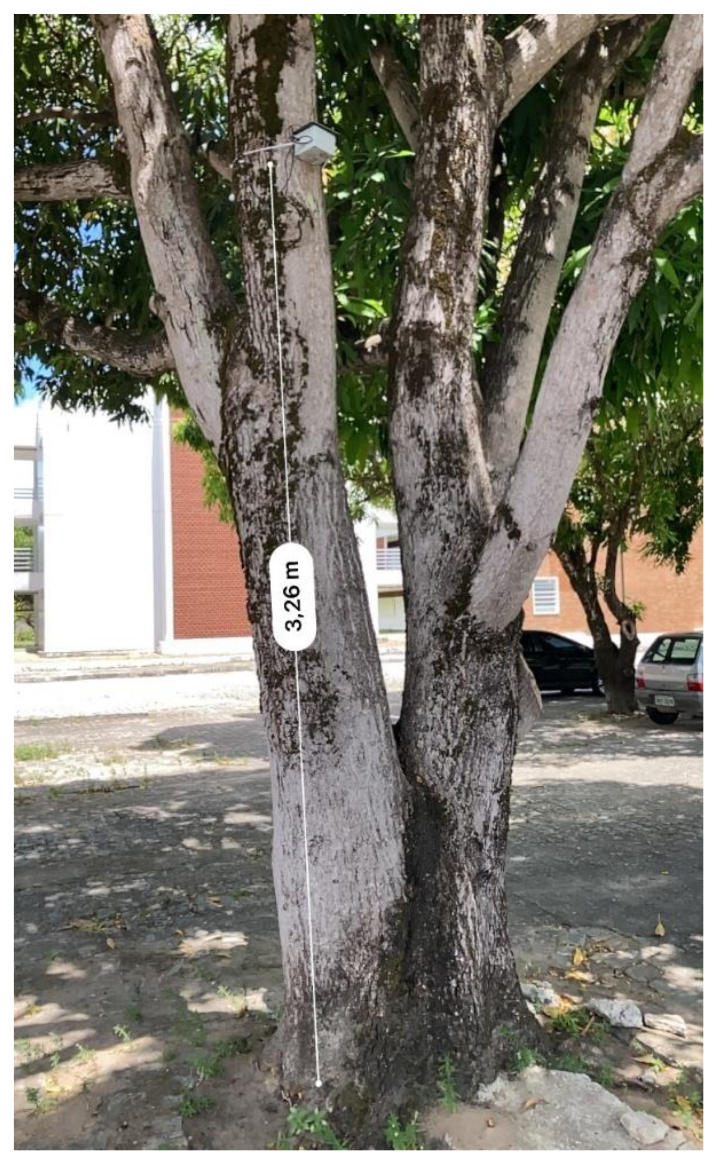
Figure 4.
Time series measured by sensors installed on the tree.
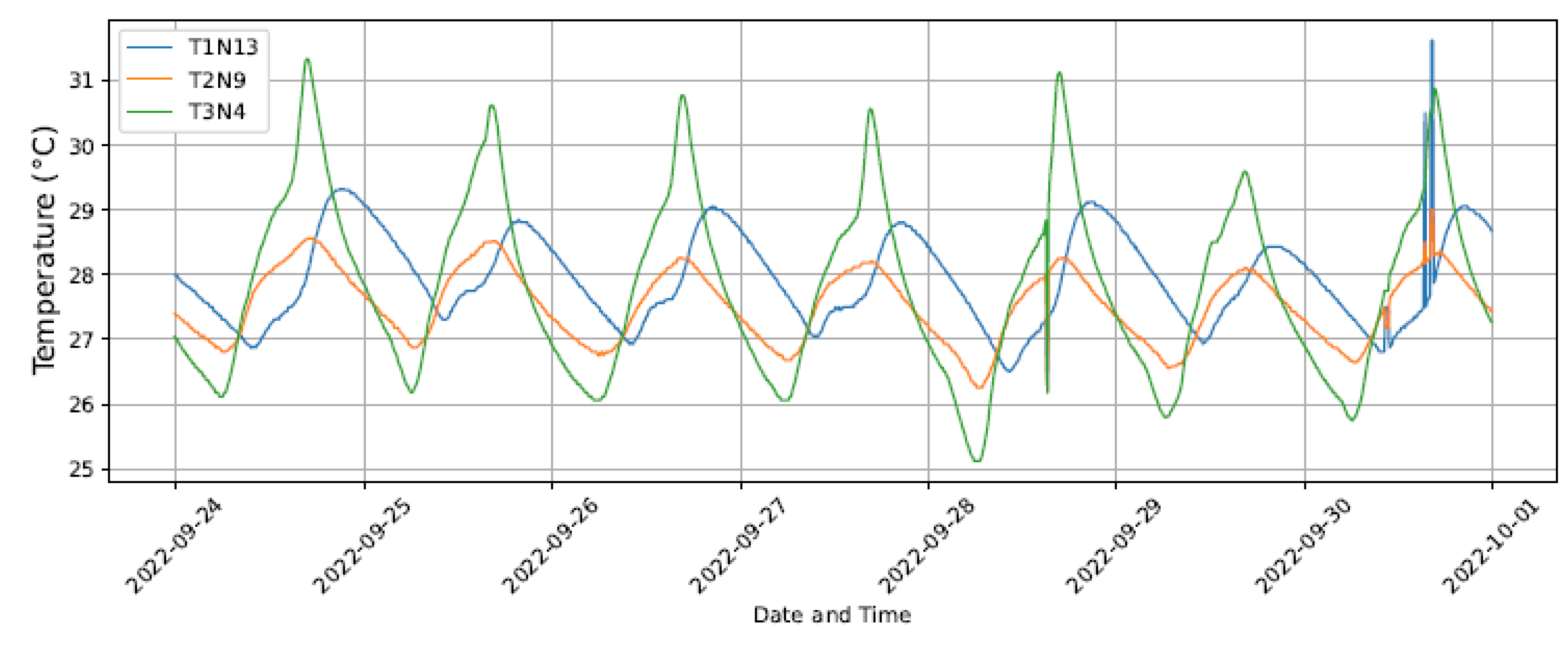
Figure 5.
Sensor–gateway communication.
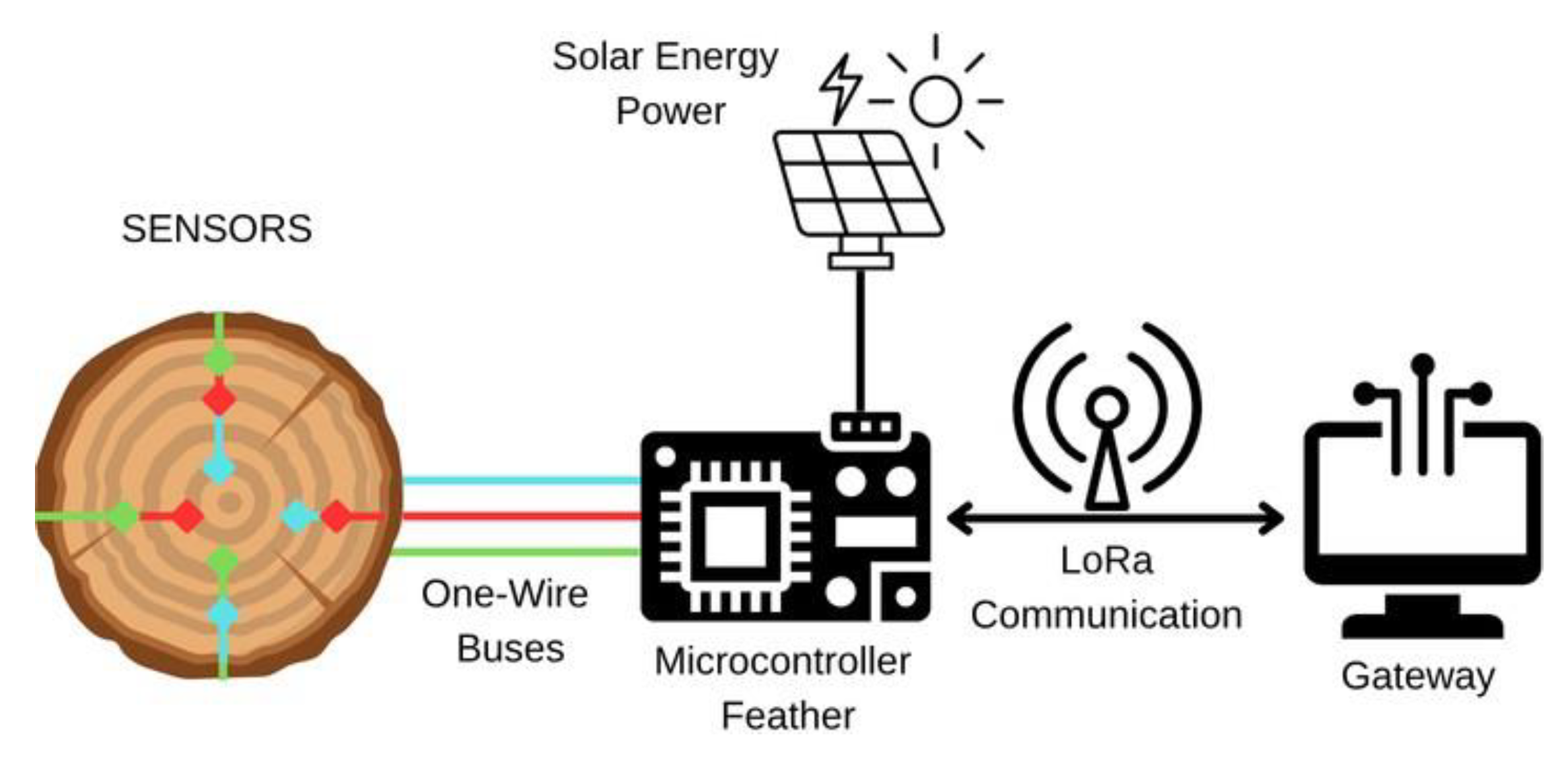
Figure 6.
CEAR weather station model.
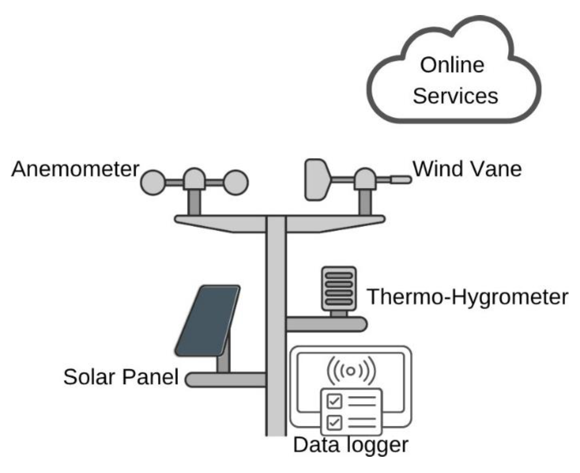
Figure 7.
Time series of wind speed and direction measured by the CEAR/UFPB automatic weather station.
Figure 7.
Time series of wind speed and direction measured by the CEAR/UFPB automatic weather station.
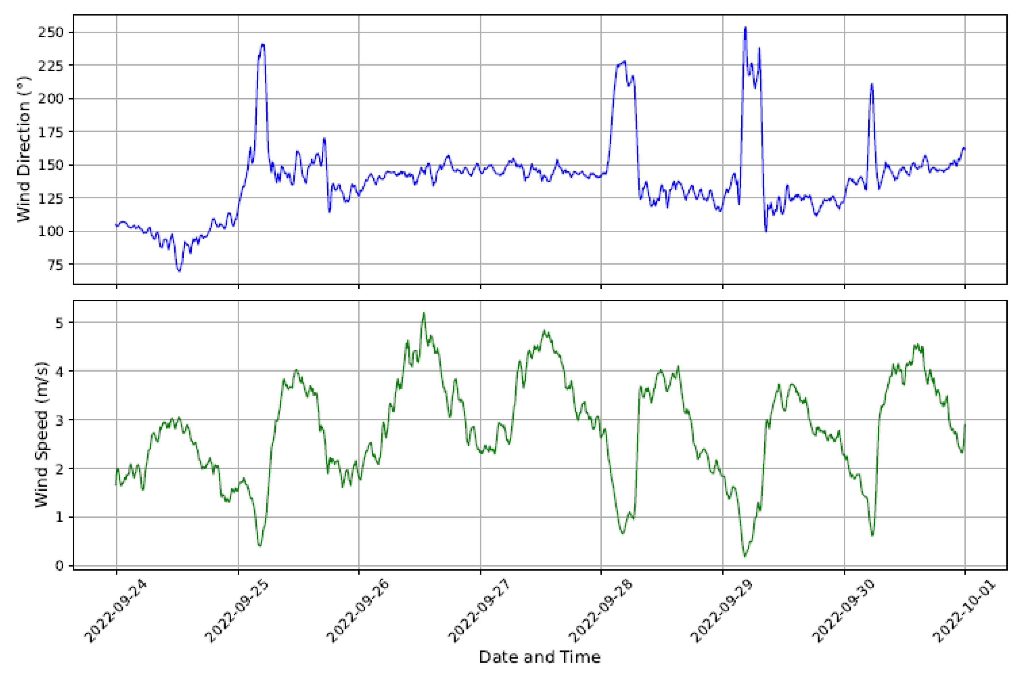
Figure 8.
Proposed methodology.
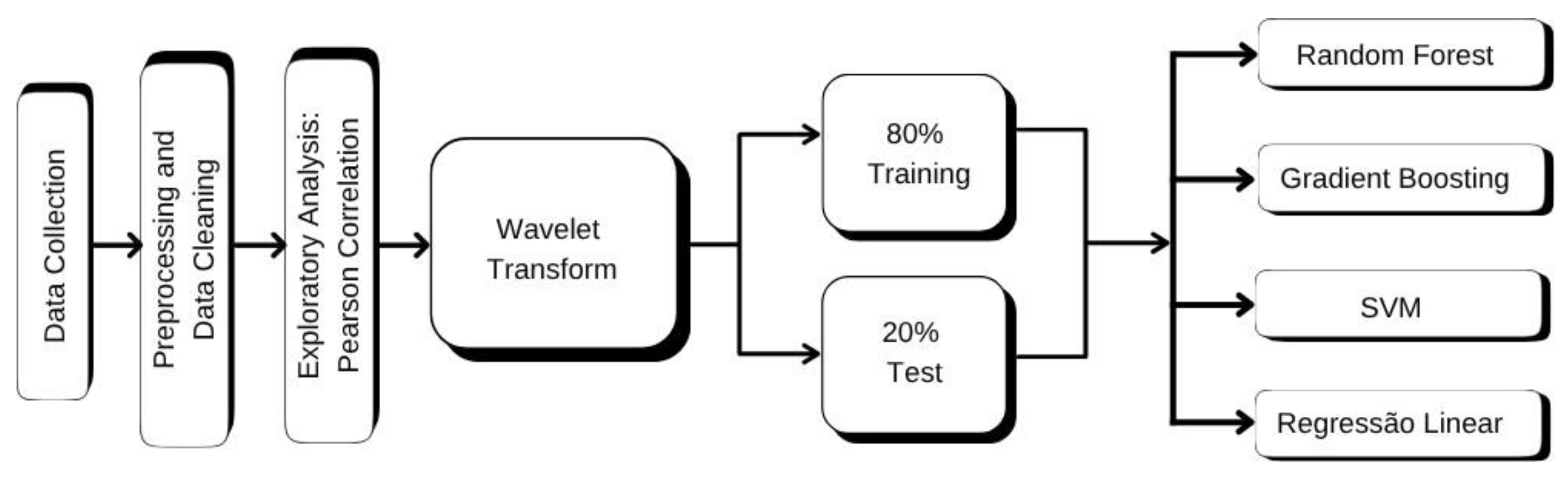
Figure 9.
Discrete Wavelet Transform model.
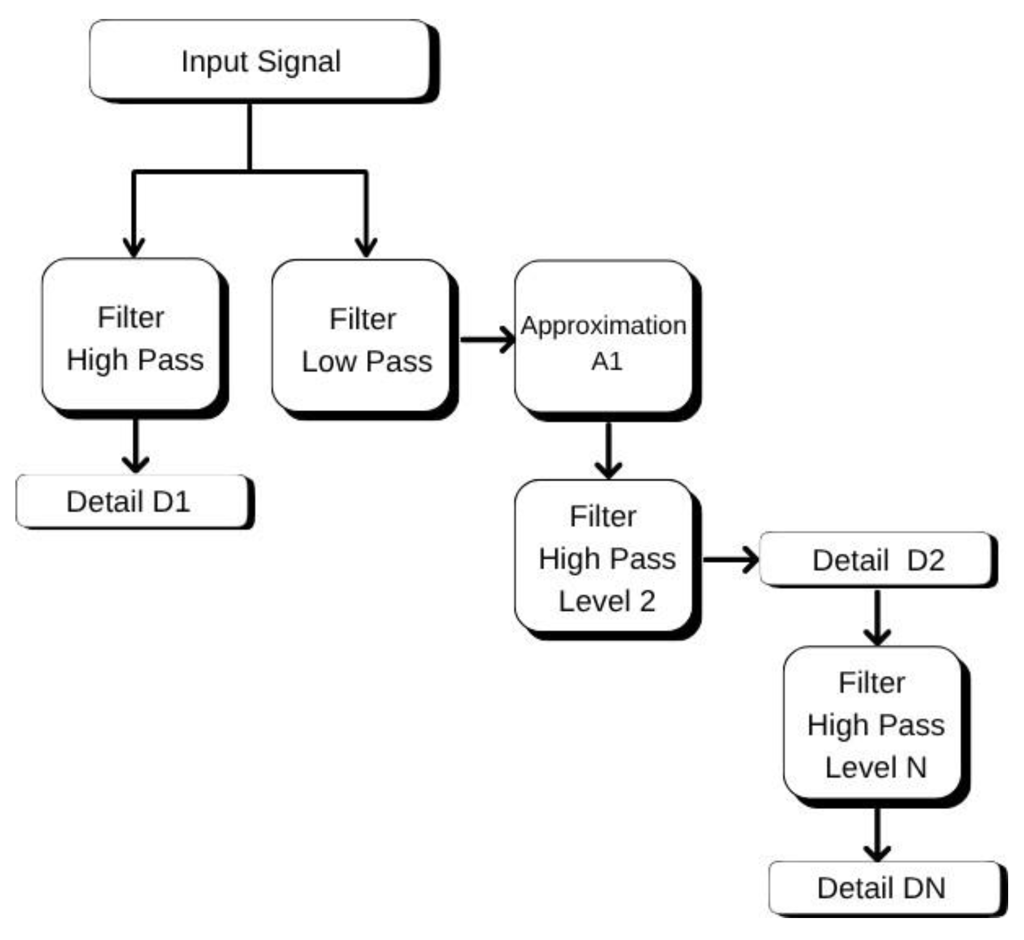
Figure 10.
Random forest model.
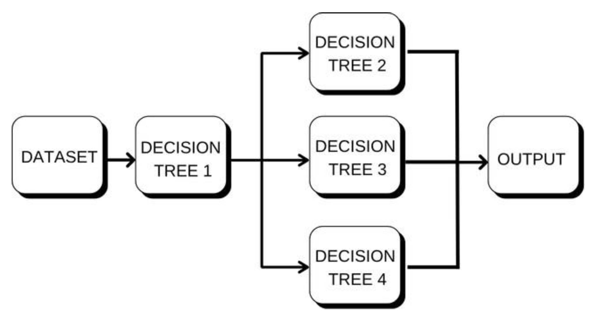
Figure 11.
Gradient boosting model.
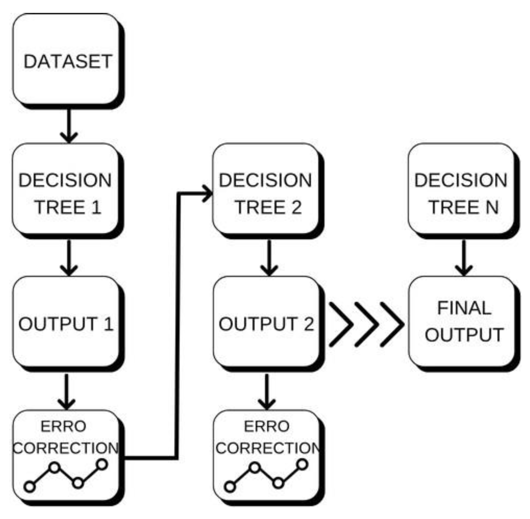
Figure 12.
SVM model.
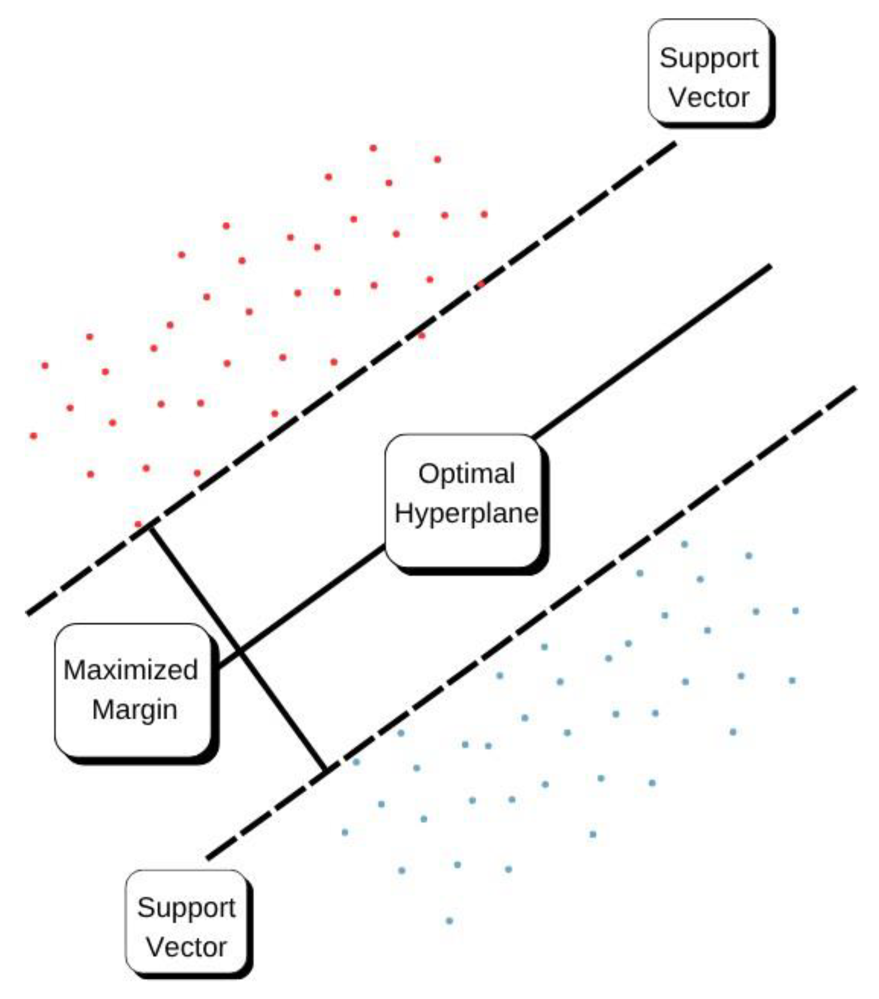
Figure 13.
Comparison between approximation coefficients.
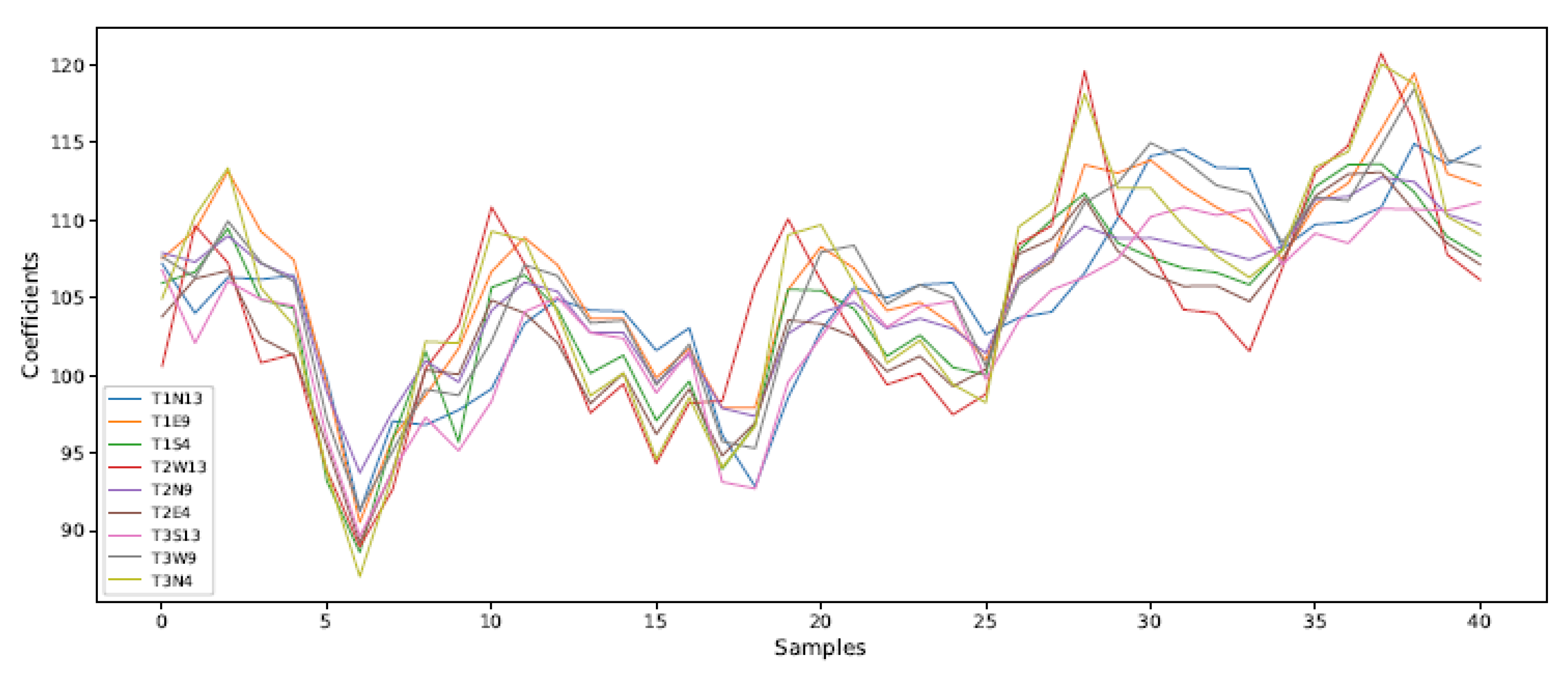
Figure 14.
Wind speed forecast comparison.
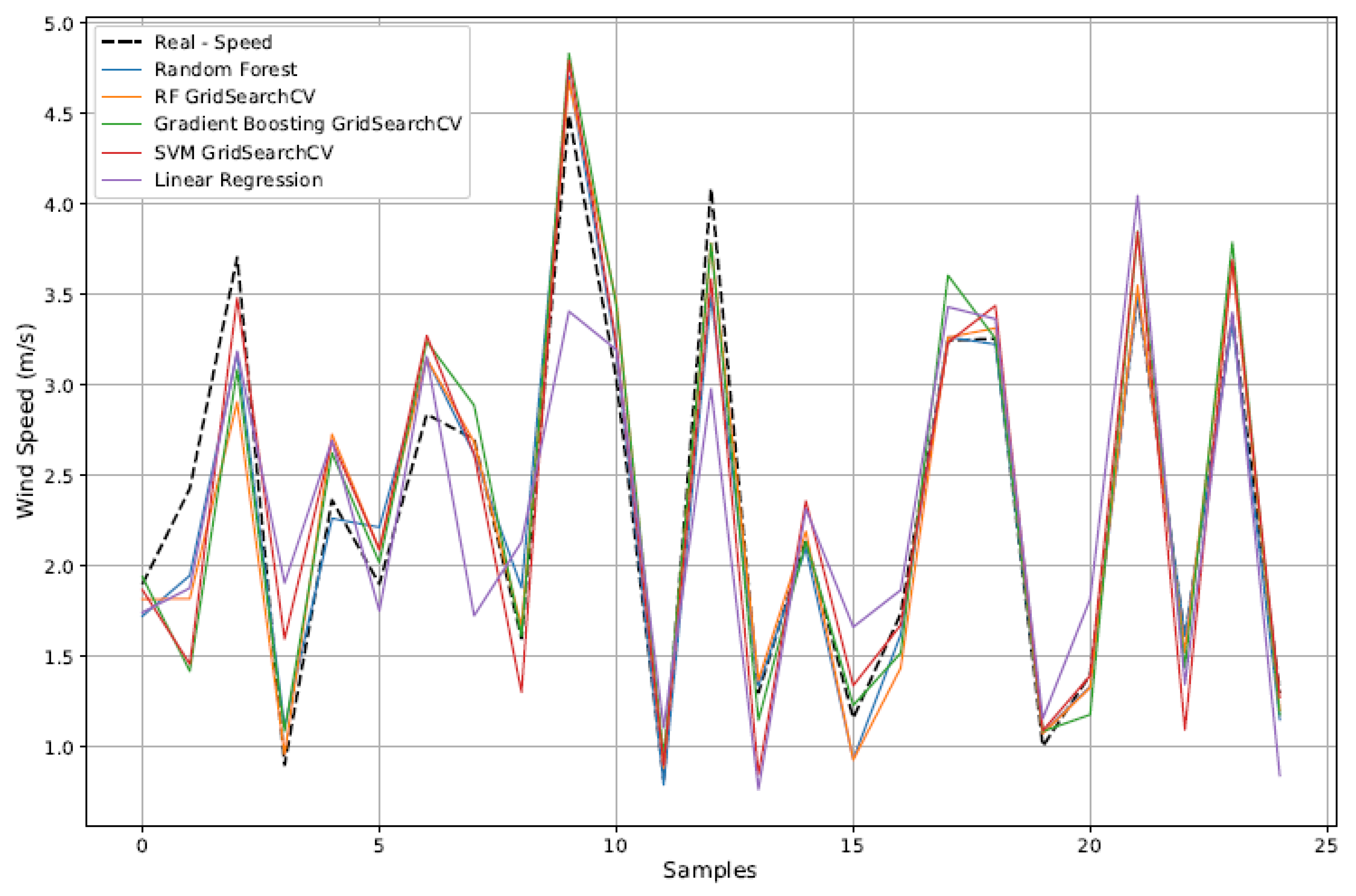
Figure 15.
Wind direction forecast comparison.
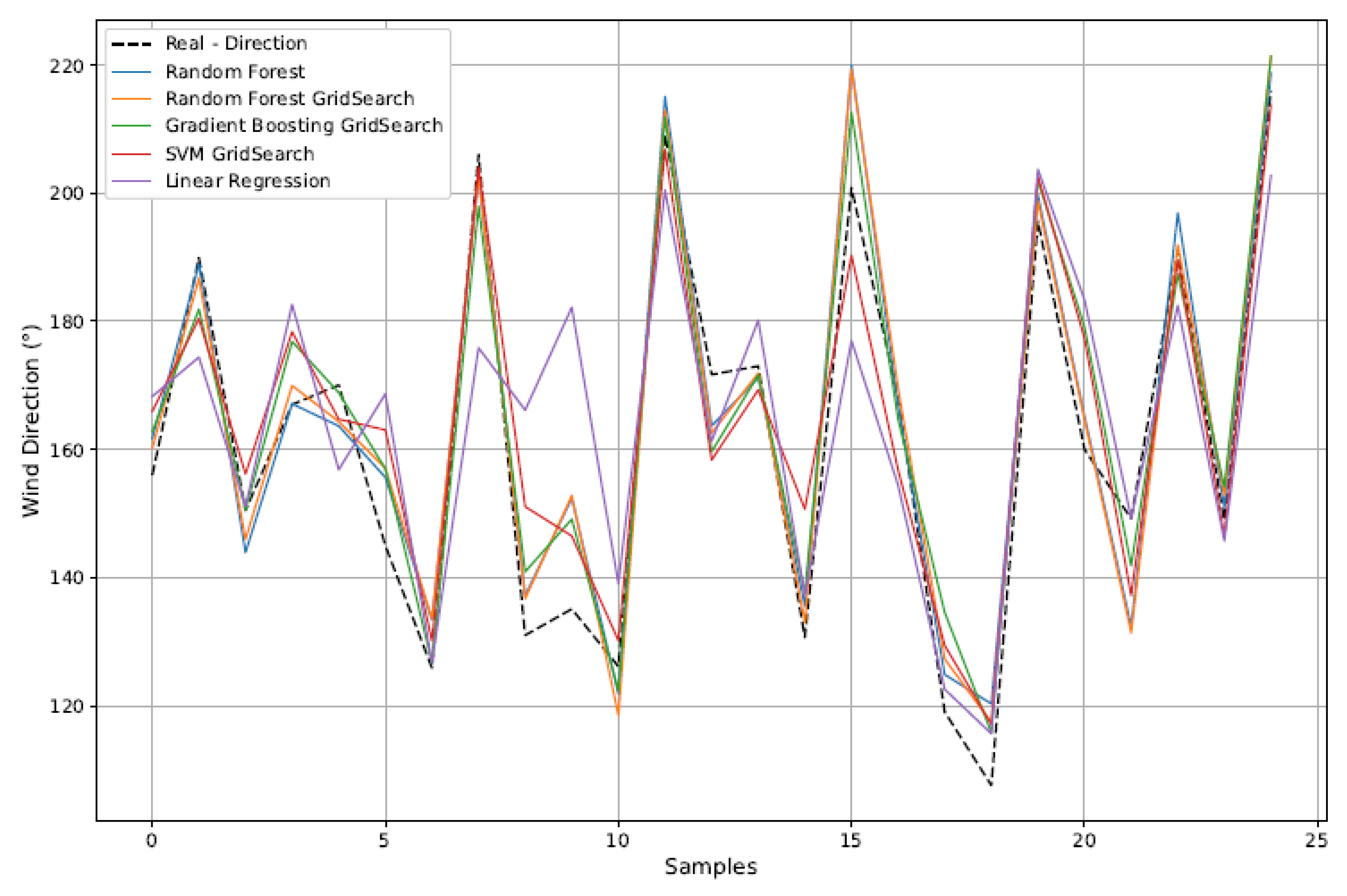

Table 1.
Distribution of temperature sensors.
| Sensor | Height | Direction | Depth |
|---|---|---|---|
| T1N13 | 1 m | North | 13.5 cm |
| T1E9 | 1 m | East | 9.0 cm |
| T1S4 | 1 m | South | 4.5 cm |
| T2W13 | 2 m | West | 13.5 cm |
| T2N9 | 2 m | North | 9.0 cm |
| T2E4 | 2 m | East | 4.5 cm |
| T3S13 | 3 m | South | 13.5 cm |
| T3W9 | 3 m | West | 9.0 cm |
| T3N4 | 3 m | North | 4.5 cm |
The label of each sensor follows the pattern Th De , where h is the height (m), D is the direction, and e is the depth (cm). For example, T1E9 is a sensor installed at 1 m height, on the East side, and 9.0 cm deep into the tree trunk.
Table 2.
Correlation between DWT coefficients and wind variables.
| Sensor Level | Direction | Speed |
|---|---|---|
| T1N13 | 0.5160 | 0.1800 |
| 1 | 0.0253 | -0.0687 |
| T1E9 | 0.4386 | 0.1580 |
| 1 | -0.0011 | 0.0141 |
| T1S4 | 0.4191 | 0.1421 |
| 1 | 0.0397 | 0.0320 |
| T2W13 | 0.3686 | 0.1548 |
| 1 | -0.0593 | -0.0063 |
| T2N9 | 0.4526 | 0.1528 |
| 1 | 0.0187 | -0.0234 |
| T2E4 | 0.4514 | 0.1741 |
| 1 | -0.0309 | -0.0030 |
| T3S13 | 0.5229 | 0.1723 |
| 1 | 0.0068 | -0.0128 |
| T3W9 | 0.5147 | 0.1762 |
| 1 | 0.0377 | 0.0085 |
| T3N4 | 0.4271 | 0.1489 |
| 1 | -0.0744 | -0.0007 |
Table 3.
Wind speed model performance.
| Model | MSE | R2 | MAPE |
|---|---|---|---|
| RF (no optimization) | 0.189 | 0.839 | 18.53% |
| RF (optimized) | 0.172 | 0.854 | 16.44% |
| GB (optimized) | 0.232 | 0.803 | 20.96% |
| SVM (optimized) | 0.263 | 0.776 | 22.33% |
| LR | 0.537 | 0.544 | 38.27% |
Table 4.
Wind direction model performance.
| Model | MSE R2 MAPE | ||
|---|---|---|---|
| RF (no optimization) | 184.16 | 0.861 | 6.83% |
| RF (optimized) | 176.13 | 0.867 | 6.60% |
| GB (optimized) | 240.33 | 0.819 | 8.16% |
| SVM (optimized) | 460.34 | 0.653 | 10.86% |
| LR | 691.35 | 0.479 | 14.16% |
Disclaimer/Publisher’s Note: The statements, opinions and data contained in all publications are solely those of the individual author(s) and contributor(s) and not of MDPI and/or the editor(s). MDPI and/or the editor(s) disclaim responsibility for any injury to people or property resulting from any ideas, methods, instructions or products referred to in the content. |
© 2025 by the authors. Licensee MDPI, Basel, Switzerland. This article is an open access article distributed under the terms and conditions of the Creative Commons Attribution (CC BY) license (http://creativecommons.org/licenses/by/4.0/).
Copyright: This open access article is published under a Creative Commons CC BY 4.0 license, which permit the free download, distribution, and reuse, provided that the author and preprint are cited in any reuse.


