
Submitted:
09 October 2025
Posted:
13 October 2025
You are already at the latest version
Abstract
In this paper we prove the existence and unicity of the minimum risk equivariant
estimator (MIRE) for the univariate linear normal models, under the action
of the subgroup of the affine group which leaves the column space of the design
matrix invariant and using the framework of the intrinsic analysis of statistical estimation
which uses the square of the Rao distance as the loss function, which
expectation behaves very different to the corresponding of the square error loss
when we work with small samples, and supplying also an intrinsic bias measure
for any equivariant estimator. This estimator is studied and compared with the
standard maximum likelihood estimator (MLE) in terms of its intrinsic risk and
bias, showing explicitly its differences, apparent with small samples, fortunately
small for large sample sizes. Moreover, an approximate and very simple estimator
is also suggested, which reduces the majority of bad behaviour of MLE, of intrinsic
risk and bias, for small samples.
Keywords:
Equivariant estimator
; Information metric
; Riemannian risk
; Intrinsic bias
1. Introduction
The Fisher information matrix of a regular parametric family of probability distributions induces a natural Riemannian structure on the parameter space [1,2,3]. This structure provides the foundation for the intrinsic analysis of statistical estimation, see [4,5] and, beyond statistics, it has also been shown to reveal connections with physical laws [6].
In this intrinsic framework, estimators are assessed through tools that do not depend on any particular parametrization of the model. Consequently, non-intrinsic criteria such as the squared error loss should be replaced by intrinsic measures. A natural choice is the squared Riemannian (Rao) distance, which serves as an intrinsic loss function. The associated risk can behave very differently from that based on squared error loss, especially in small-sample regimes. Similarly, the classical definition of bias must be reformulated in terms of a vector field determined by the geometry of the model, whose squared norm provides a natural intrinsic bias measure.
The estimator itself should also be intrinsic, i.e., independent of parametrization. Consider, for instance, the exponential distribution under two parametrizations,
where is the positive real numbers indicator. The UMVU estimator computed under each parametrization and are not related by . This apparent inconsistency arises because UMVU estimators rely on non-intrinsic notions such as unbiasedness and variance. As a result, the UMVU estimator is parametrization-dependent and cannot be regarded as intrinsically defined.
When the statistical model is invariant under the action of a transformation group on the sample space, it is natural to restrict attention to equivariant estimators, i.e., estimators U satisfying
where is the transformation group acting on the space of all samples of size n and is the induced transformation on the parameter space . This restriction ensures logical consistency: only equivariant estimators remain coherent under data transformations. It is therefore a requirement that should be imposed prior to any attempt to minimize an intrinsic risk function.
As an illustration, consider the estimation of the unconstrained mean of a p–variate normal distribution. The MLE of (which really defines and intrinsic estimator) based on a sample of size n, is just the sample mean vector . However, for , the James–Stein estimator is known to have smaller quadratic risk [7]. In our view, this does not undermine the MLE. Although the James–Stein estimator enjoys a lower risk under the non-intrinsic quadratic loss, it lacks the essential property of equivariance, which is crucial from the intrinsic perspective.
In this work we focus on classical statistical estimation, as is standard in the absence of prior knowledge. Nonetheless, intrinsic Bayesian approaches based on non-informative priors are also possible [5,8], and represent an interesting avenue for future research. Here, we adopt the squared Rao distance as a natural loss function, since it is the conceptually simplest intrinsic analogue of the quadratic loss, despite potential computational challenges. For a broader background on statistical estimation and its intrinsic developments, see [9,10,11,12].
Specifically, we consider the univariate linear normal model with a fixed design matrix. First, we explicitly characterize the class of equivariant estimators under the action of a suitable subgroup of the affine group–namely, those affine transformations of the data that leave the column space of the design matrix unchanged. This subgroup is the largest one that preserves the model’s structure. Next, we prove the existence and uniqueness of the estimator within this class that minimizes intrinsic risk, i.e., the equivariant estimator that minimizes the mean squared Rao distance. We also derive an explicit expression for the intrinsic bias of any equivariant estimator.
Furthermore, we compare the intrinsic bias and risk of the proposed estimator with those of the MLE, highlighting their differences in small samples and showing how these differences diminish as the sample size grows. Finally, we propose a computable approximation of the optimal estimator, which mitigates most of the intrinsic bias and risk issues that affect the MLE in finite samples.
2. Equivariant estimators for linear models
Let us consider the univariate linear normal model,
where is a random vector, is a matrix of known constants with , is a vector of unknown parameters to be estimated and is the fluctuation or error of about . We assume that the errors are unbiased, independent, with the same variance and following a n–variate normal distribution, that is , where is the identity matrix. Therefore distributes according to an element of the parametric family of probability distributions with parameter space , a – dimensional simply connected real manifold. Hereafter, we shall identify the elements of with column vectors, when necessary.
Denote by
where E is a subspace of and is the group of orthogonal matrices with entries from . Define F as the subspace of spanned by the columns of , that is . Observe that , , and if then . Moreover, every induces, in F and , two isomorphisms isomorphisms preserving the Euclidean norm in each subspace.
is invariant under the action of the subgroup of the affine group in given by the family of transformations
where .
Observe that induces an action on the parameter space given by
where this result is obtained taking into account that is the projection matrix into F and thus, if there exists a unique such that and .
Since the family is invariant under the action of , it is natural to restrict our attention to the class of equivariant estimators of i.e. an estimator satisfying for all .
Proposition 1.
Let be an equivariant estimator of . Then belongs to the family where,
Proof. Let . The equivariance condition for involves,
for any .
Any can be written in a unique form as where and . Specifically
If we choose in the previous expressions, we obtain
First we focus on . If we let , we have with
Now observe that (5) is satisfied for any and in , in particular for and . Therefore
But which leads to
From (4),
Next, we consider . Let and in (), it follows
Accordingly, it is enough to determine on . Let us take a unit vector such that . Then ().
for any . Observe that any arbitrary unit vector in can be written as for a proper . Therefore, for any , , we have
Observe also that if then and, choosing , we have that . This implies .
□
Observe that the standard maximum likelihood estimator, MLE, for the present model is an equivariant estimator, with .
3. Minimum Riemannian risk estimators
In the framework of intrinsic analysis, where the loss function is the square of the Rao distance, the Riemannian distance induced by the information metric in the parameter space , once the class of the equivariant estimators has been determined a natural question arises: which is the equivariant estimator that minimizes the risk?
First of all, we summarize the basic geometric results corresponding to the model (1) which are going to be used hereafter. We are going to use a standardized version of the information metric, given by the usual information metric corresponding to this linear model divided by a constant factor n, i.e. the number of rows of matrix . This metric is given by
which is, up to a linear coordinate change, the Poincaré hyperbolic metric of the upper half space , see [13]. The Riemannian curvature is constant and negative and the unique geodesic, parameterized by the arc–length, which connects two points and , when , is given by:
where s is the arc–length, and are vectors whose components, and also , are convenient real integration constants, such that , , , being the Riemannian distance between and . Finally, K is given by . When , the geodesic is given by
where B is a positive integration constant.
The Rao distance between the points and is
where
and
or, equivalently,
Let be the inverse of the exponential map corresponding to Levi-Civita connection and its components corresponding to the basis field . Then, we have
It is well know that the Riemannian distance induced by the information metric is invariant under equivariant estimator transformations. We shall supply a direct and alternative proof for the linear model setting.
Proposition 2.
The Rao distance ρ given by (11) is invariant under the action of the induced group by on the parameter space, . In other words
Proof: Observe that
and taking into account that is the projection matrix into F, we have
Therefore
and the invariance of and trivially follows. □
Proposition 3.
acts transitively on Θ.
Proof: The transitivity follows observing that a is an arbitrary positive real number and is the projection matrix into F with . □
Since , and thus , is invariant under the action of and acts transitively on , the distribution of does not depend on , and therefore, the risk of any equivariant estimator remains constant and independent of the target parameter provided that this risk is finite. More precisely, observe that if we let
from (1) and (4) we clearly have that with a rank m idempotent covariance matrix, and and are independent random variables following a chi-square distribution with m and degrees of freedom, equal to the dimensions of F and since and are quadratic forms based on the projection matrices on these subspaces of and (or ) and are independent random vectors. Therefore, since and , we have that
and
or
which have a distribution which depend only on and , independent random variables with fixed distribution, whatever the value of .
Since the risk of any equivariant estimator remains constant on the parameter space, it’s enough to examine it at one point, for instance at the point . Let us denote the expectation with respect to the n–variate linear normal model by and by E the . We can prove the following propositions.
Proposition 4.
If we have:
for any .
Proof: From (14) and (13), since
we have
developing the square of the difference and taking into account that the standard Euclidean norm of a vector is less or equal to the absolute value of the sum of its components, we obtain
Notice that both bounds (22) and (23) are invariant under the action of the induced group on the parameter space.
As we mentioned before, from [14], it is enough to prove that the risk is finite at . Taking into account (16) it follows, from (23), that
Observe that if Q has a chi-square distribution with k degrees of freedom
Therefore, since and are independent random variables following a central chi-square distribution with m and degrees of freedom, we have
and
Then, taking the average, it follows that
Since n and m are positive integers being , we conclude that the risk is finite if . □
Proposition 4 is a sufficient condition for the existence of the Riemannian risk of the equivariant estimator , thus
is well defined for , which we shall assume hereafter.
Proposition 5.
There exists a unique minimizer of the Riemannian risk given by Φ.
Proof:
Let us consider the Riemannian risk at as a function of s, that is
The particular selection of , from which F follows, relies on the Riemannian structure of induced by the information metric. The Riemannian curvature is constant and equal to and taking into account (10) we have that
is a geodesic in ; precisely a geodesic parameterized by the arc–length, see [13] for further details.
Then, following [15], the real valued function
is strictly convex. Since almost surely convexity of a stochastic process carries over the mean of a process, the map F is strictly convex as well.
On the other hand, from Fatou’s Lemma as or . This, together with the strict convexity of F yield the existence of a unique minimizer of the function F, which depends on n and m.
Finally, since the map is a strictly monotonous function; must exist a unique , namely , such that . □
In fact, this result guarantees the unicity of the MIRE, although a numerical analysis is required to obtain it explicitly (see next section). It could be useful to develop a simple approximate estimator, that shall be referred hereafter a-MIRE, obtained, luckily, minimizing a convenient upper bound of . Since
we shall have
and therefore
the upper bound it is clearly a convex functions with an absolute minimum attained when satisfy
Furthermore, given an arbitrary m, we have
and, therefore, a-MIRE is very close to MLE for large values of n. Observe also that it is possible to compute a-MIRE for , a condition which is slightly stronger that the result required for the existence of MIRE in proposition (4).
A further aspect is the intrinsic bias of the equivariant estimators. In fact connections between minimum risk, bias and invariance have been established, see [14]. Since the action of the group G is not commutative, we cannot guarantee the unbiasedness of the MIRE and an additional analysis must be performed. First of all we are going to compute the vector bias, see [4], a quantitative measure of the bias which is compatible with Lehmann results.
Let and be the components of corresponding to the basis field , . With matrix notation, . Furthermore, let us define for and ; taking into account (16), (19) and from (11) and (15) we have
where
and
Let be the intrinsic bias vector corresponding to an equivariant estimator evaluated at the point and let be their components. In matrix notation, . We have
Proposition 6.
If , the bias vector is finite and
where and are independent random variables following a chi-square distribution with m and degrees of freedom respectively.
Moreover, the square of the norm of the bias vector is constant and given by
Proof: Observe that if we have
where denotes the Riemannian norm at the tangent space at .
On the other hand taking into account (31) and defining as in (16) observe that , is independent of and and has the same distribution. Then we have
and since it follows that .
is obtained directly from (31). The distribution of and follow from basic properties of multivariate normal distribution. Finally, the norm of the bias vector field follows from (32) and (8).
□
We may remark, finally, that the norm of the bias vector field of any equivariant estimator, , is invariant under the action of the induced group, , on the parameter space and since this group acts transitively on , this quantity must be constant, which is clear from (33).
4. Numerical Evaluation
In this section we are going to compare, numerically, the MIRE estimator with the standard MLE. Observe that both estimators only differ in the estimation of the parameter (or ). Precisely, the MIRE and the MLE of are, respectively,
namely, they only differ by the factor , since .
In order to compare MLE with the MIRE we have computed the factor , the intrinsic risk and the square of the norm of the bias vector for each estimators. All the computations have been performed using Mathematica 10.2.
Moreover, we have suggested a rather simple approximation for , or , which allow us to approximate MIRE estimator through (29), i.e.
The corresponding estimator, that shall be referred hereafter as a-MIRE, has been also compared with MLE and MIRE in terms of intrinsic risk.
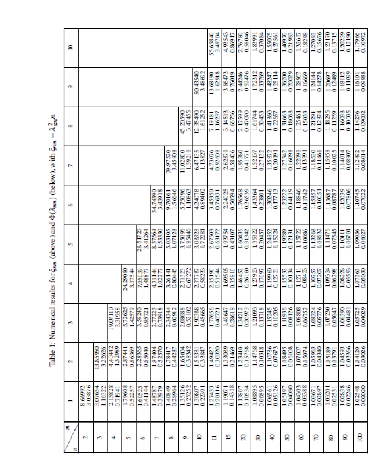
The results are summarized in the following figures which summarize the tables given in the Appendix, see [16] for a convincing argument for the use of plots over tables. In Figure 1 numerical results of (left) and (right) are displayed graphically. Observe that, for m fixed, as n increases goes to zero and goes to one. The exact numerical values are given in the Appendix, Table 1.
Figure 1.
Numerical results for (left) and (right), with .
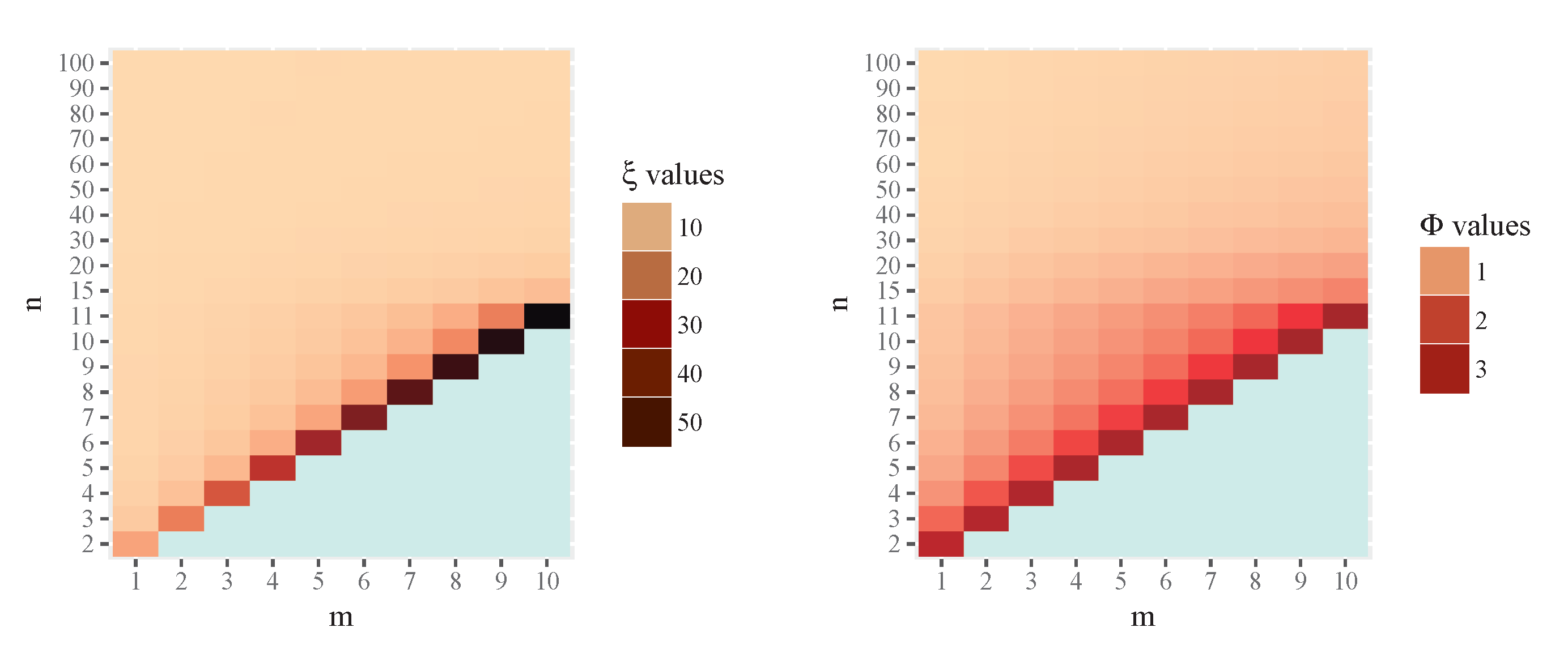
Figure 2.
Numerical results for (left) and (right), with .
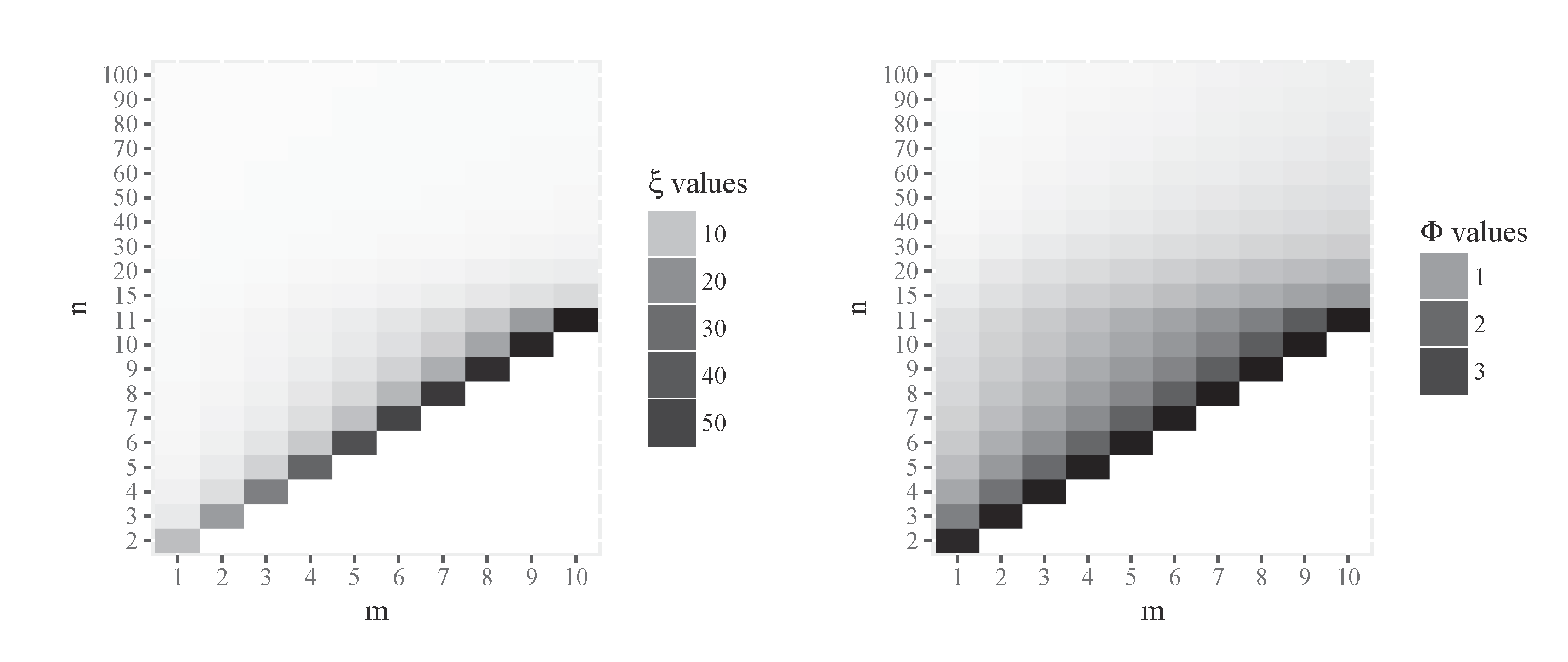
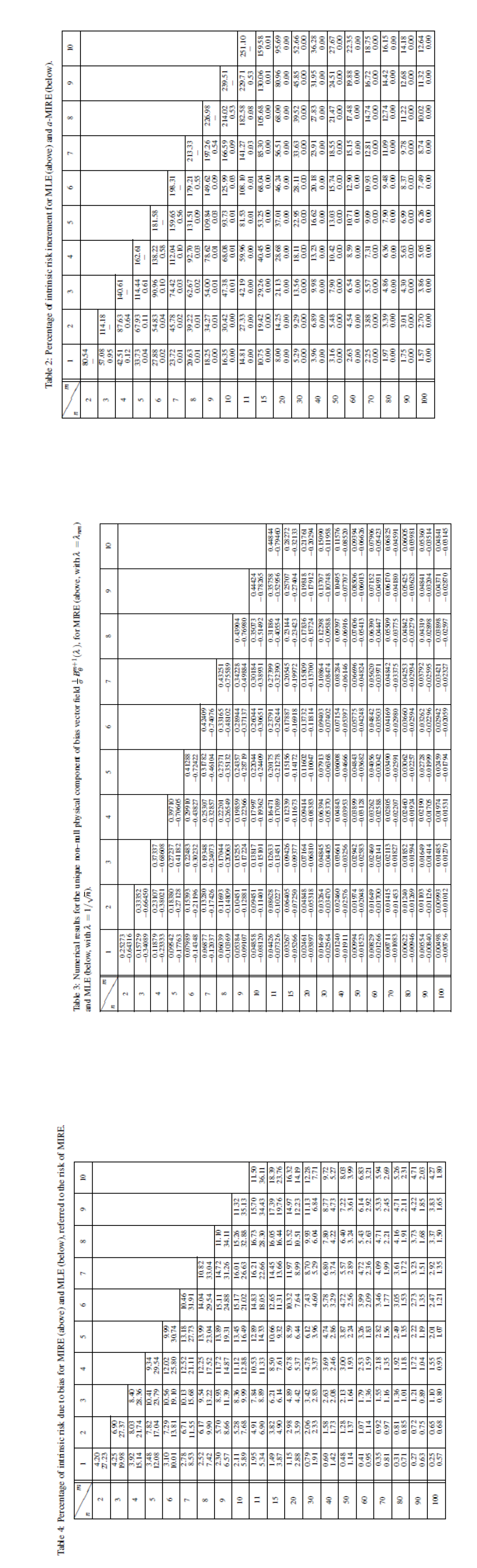
Figure 3 shows graphically the percentage of intrinsic risk increment for MLE (left) and a-MIRE (right), that is
respectively, for some values of n and m. The exact numerical results are given in the Appendix, Table 2.
Observe that if we approximate the MIRE by the MLE for a certain value of m, the relative difference of risk decreases as n increases. Notice that these relative differences of risks are rather moderate or small (about 10-15%) only if . Let us remark also the non appropriate behavior of the MLE for small values of . This regards to the intrinsic risk increment: when we use MLE instead of MIRE this increment oscillates between and when with m from 1 to 10. On the other hand, the behavior of the a-MIRE is reasonably good, with its intrinsic risk very similar to the risk of the MIRE estimator: here the percentage on risk increment is less than for all studied cases and also this percentage decreases as n increases. In fact this percentage is lower than 1‰ when , which indicates the extraordinary degree of approximation, being therefore the a-MIRE a reasonable and useful approximation of MIRE. In particular as an example, for a two way analysis of variance, with a and b levels for factors A and B respectively, with a single replicate for treatment we shall have
with and , while the corresponding quantity for MLE is .
In particular if and we shall have
and , which is sensibly different. At this moment, it could be useful to recall that the quadratic loss and the squared of the Riemannian distance behaves very different, see [5].
Figure 3.
Percentage of intrinsic risk increment for MLE (left) and a-MIRE (right).
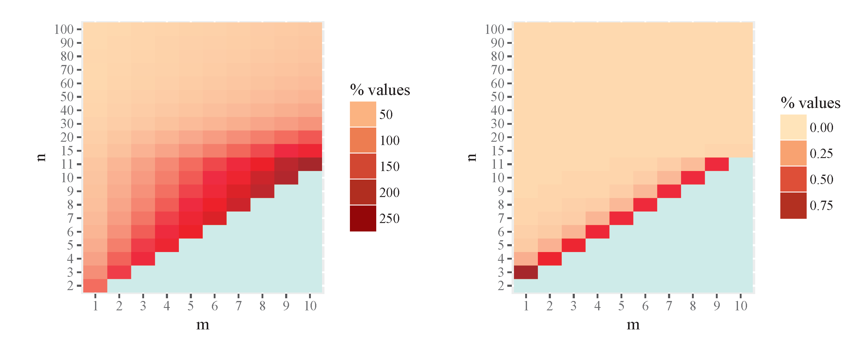
Figure 4.
Percentage of intrinsic risk increment for MLE (left) and a-MIRE (right).
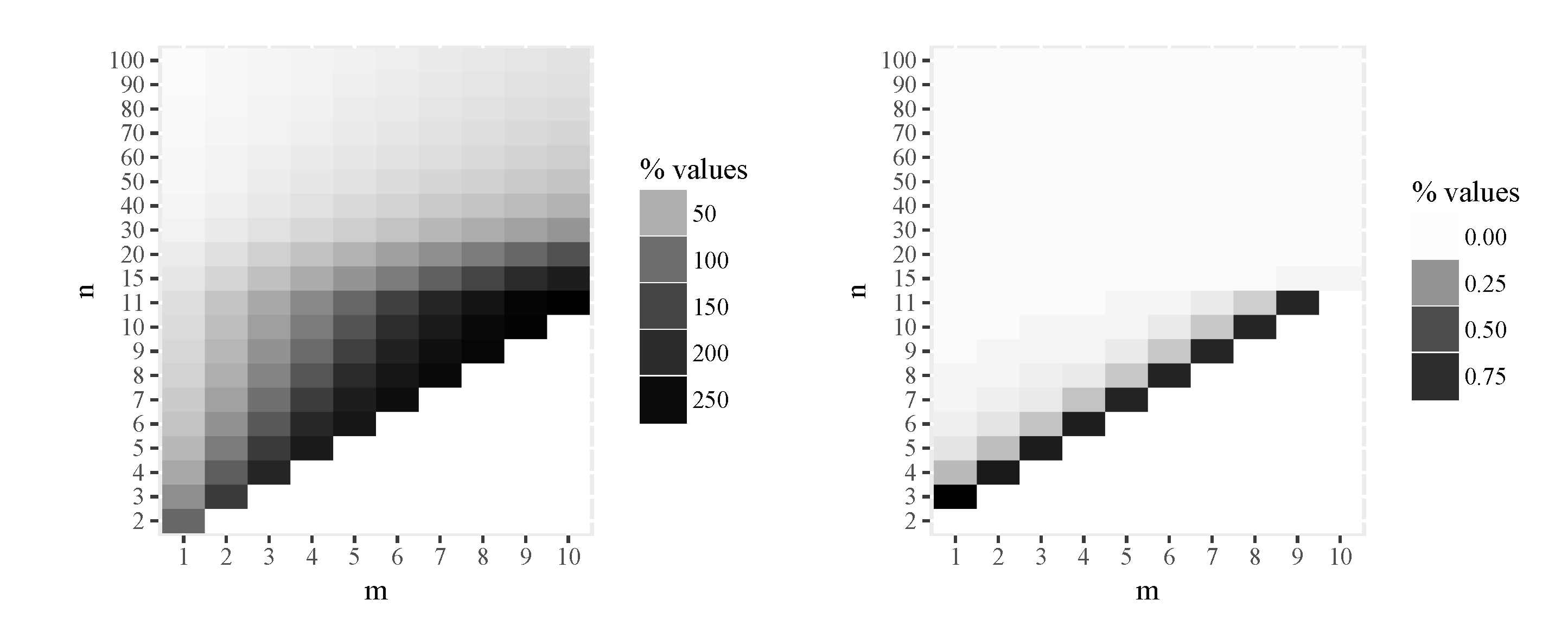
Figure 5 displays graphically the numerical results of the component of the bias vector divided by , i.e. the unique non zero physical component of this vector field, for MIRE (left) and MLE (right), and respectively, for some values of n and m. Observe the sign differences, meaning that MIRE overestimates, in average, while MLE underestimates this quantity, in average as well. This follows from the equation of the geodesics of the present model (9). The exact numerical values are given in the Appendix, Table 3.
Figure 5.
Numerical results for the unique non–null physical component of bias vector field , for MIRE (left, with ) and MLE (right, with ).
Figure 5.
Numerical results for the unique non–null physical component of bias vector field , for MIRE (left, with ) and MLE (right, with ).
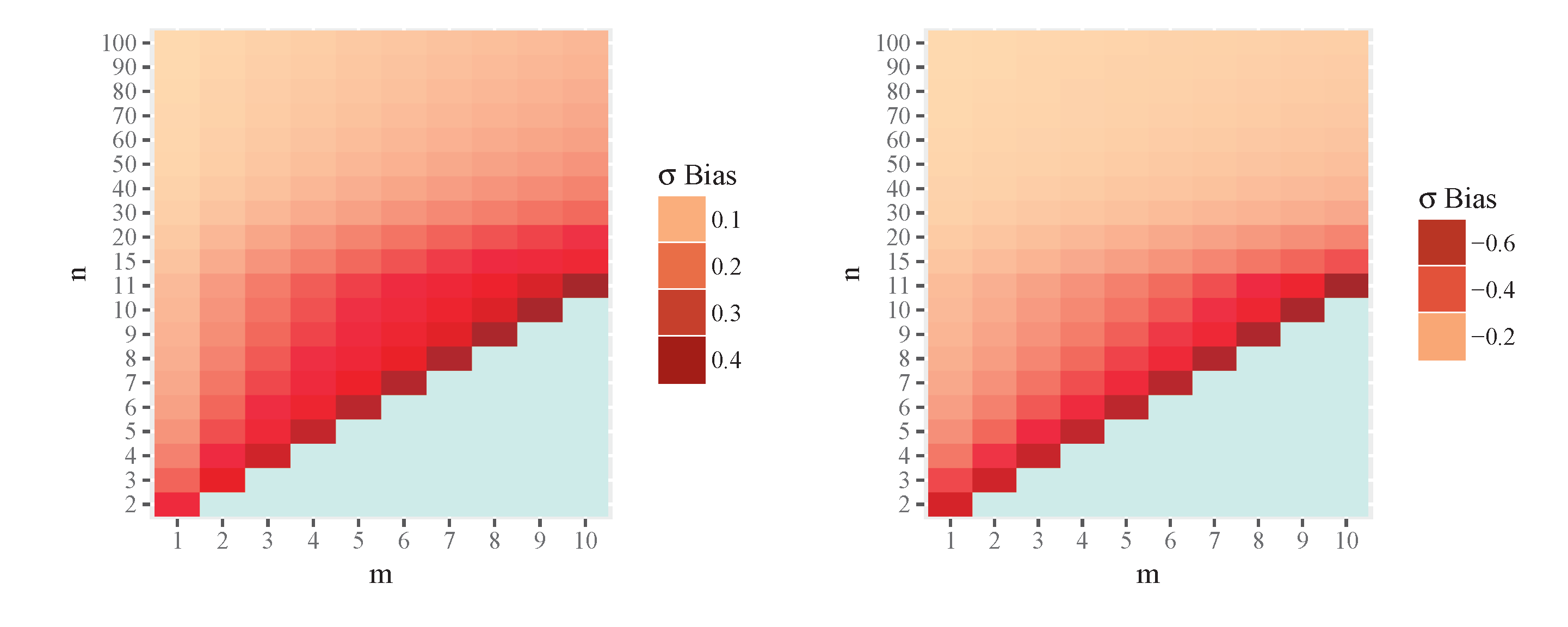
Figure 6.
Numerical results for the unique non–null physical component of bias vector field , for MIRE (left, with , positive values) and MLE (right, with , negative values).
Figure 6.
Numerical results for the unique non–null physical component of bias vector field , for MIRE (left, with , positive values) and MLE (right, with , negative values).
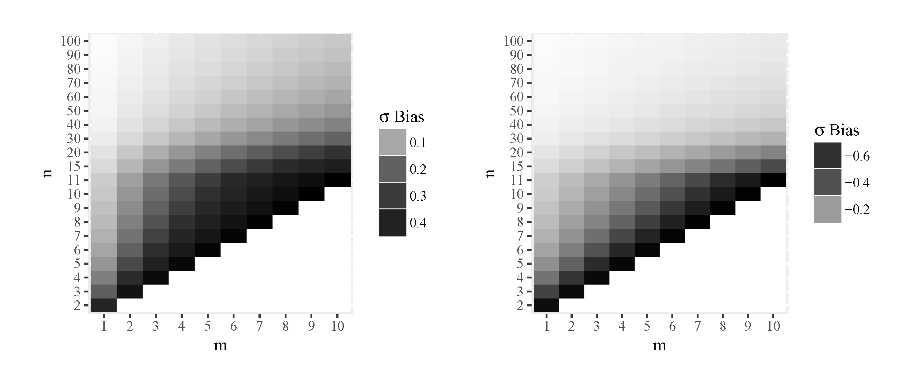
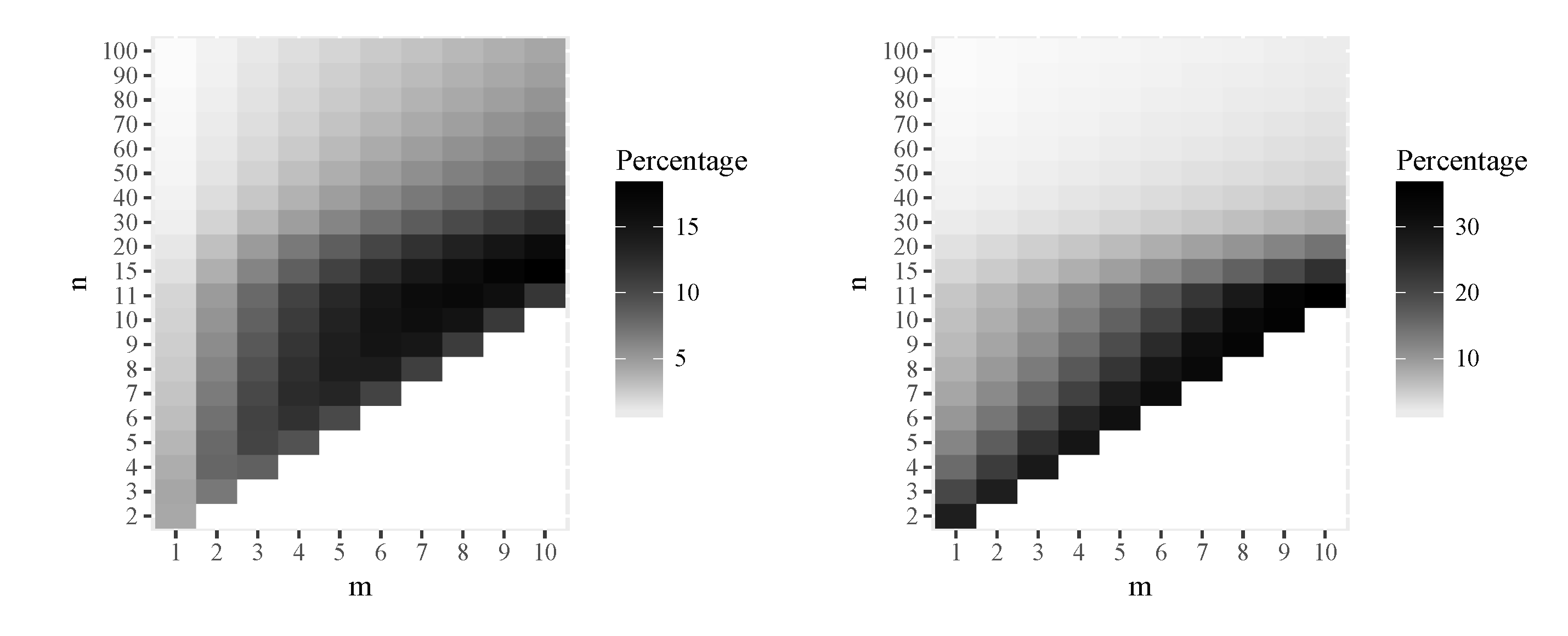
Figure 7 shows graphically the numerical results of the percentage of intrinsic risk due to bias for MIRE and MLE, that is
respectively, for some values of n and m. Observe that the bias is moderate, with respect the intrinsic risk, in both estimators. The bias of MIRE estimator is smaller than the bias of MLE for small values of m and the opposite for large values. The exact numerical results are given in the Appendix, Table 4.
Figure 7.
Percentage of intrinsic risk due to bias for MIRE (left) and MLE (right), referred to the risk of MIRE.
Figure 7.
Percentage of intrinsic risk due to bias for MIRE (left) and MLE (right), referred to the risk of MIRE.
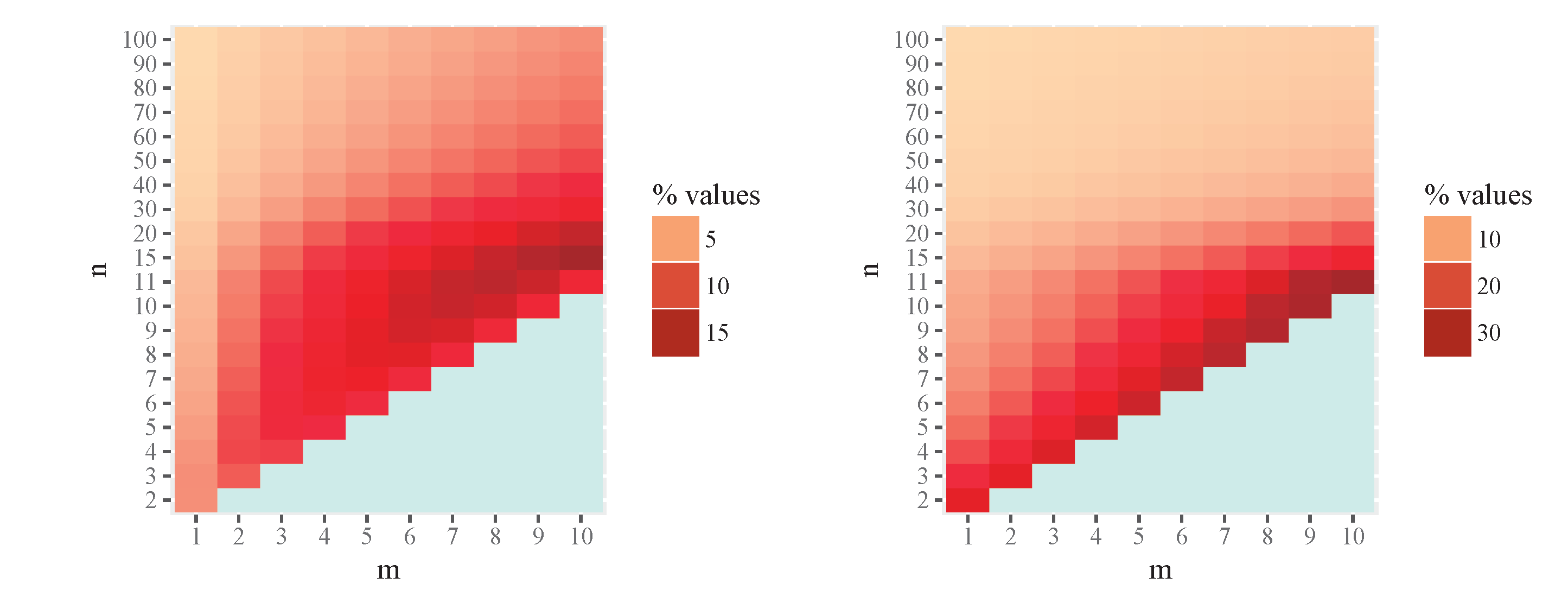
Figure 8.
Percentage of intrinsic risk due to bias for MIRE (left) and MLE (right), referred to the risk of MIRE.
Figure 8.
Percentage of intrinsic risk due to bias for MIRE (left) and MLE (right), referred to the risk of MIRE.
Acknowledgements: We have to thank the referees and the editor comments and suggestions for the improvement of this paper.
Appendix
References
- Rao, C. Information and accuracy attainable in the estimation of statistical parameters. Bull. Calcutta Math. Soc. 1945, 37, 81–91. [Google Scholar]
- Burbea, J.; Rao, C. Entropy differential metric, distance and divergence measures in probability spaces: a unified approach. J. Multivar. Anal. 1982, 12, 575–596. [Google Scholar] [CrossRef]
- Burbea, J. Informative geometry of probability spaces. Expo. Math. 1986, 4, 347–378. [Google Scholar]
- Oller, J.; Corcuera, J. Intrinsic Analysis of the Statistical Estimation. Ann. Stat. 1995, 23, 1562–1581. [Google Scholar] [CrossRef]
- García, G.; Oller, J. What does intrinsic mean in statistical estimation? Sort 2006, 2, 125–146. [Google Scholar]
- Bernal-Casas, D.; Oller, J. Variational Information Principles to Unveil Physical Laws. Mathematics 2024, 12, 3941. [Google Scholar] [CrossRef]
- Muirhead, R. Aspects of Multivariate Statistical Theory; John Wiley & Sons Inc.: New York, NY, USA, 1982. [Google Scholar]
- Bernardo, J.; Juárez, M. Intrinsic estimation. In Bayesian Statistics 7; Bernardo, J., Bayarri, M., Berger, J., Dawid, A., Hackerman, W., Smith, A., West, M., Eds.; Oxford University Press: Berlin, Germany, 2003; pp. 465–476. [Google Scholar]
- Lehmann, E.; Casella, G. Theory of Point Estimation; Springer Science & Business Media: New York, NY, USA, 2006. [Google Scholar]
- ichi Amari, S. Information Geometry and Its Applications; Springer: Tokyo, 2016. [Google Scholar]
- Ay, N.; Jost, J.; Lê, H.V.; Schwachhöfer, L. Information Geometry; Springer: Cham, 2017. [Google Scholar]
- Nielsen, F. An Elementary Introduction to Information Geometry. Entropy 2020, 22, 1100. [Google Scholar] [CrossRef] [PubMed]
- Burbea, J.; Oller, J. The information metric for univariate linear elliptic models. Stat. Decis. 1988, 6, 209–221. [Google Scholar] [CrossRef]
- Lehmann, E. A general concept of unbiasedness. Ann. Math. Stat. 1951, 22, 587–592. [Google Scholar] [CrossRef]
- Karcher, H. Riemannian Center of Mass and Mollifier Smoothing. Commun. Pure Appl. Math. 1977, 30, 509–541. [Google Scholar] [CrossRef]
- Gelman, A.; Pasarica, C.; Dodhia, R. Let’s practice what we preach: turning tables into graphs. Am. Stat. 2002, 56, 121–130. [Google Scholar] [CrossRef]
Disclaimer/Publisher’s Note: The statements, opinions and data contained in all publications are solely those of the individual author(s) and contributor(s) and not of MDPI and/or the editor(s). MDPI and/or the editor(s) disclaim responsibility for any injury to people or property resulting from any ideas, methods, instructions or products referred to in the content. |
© 2025 by the authors. Licensee MDPI, Basel, Switzerland. This article is an open access article distributed under the terms and conditions of the Creative Commons Attribution (CC BY) license (http://creativecommons.org/licenses/by/4.0/).
Copyright: This open access article is published under a Creative Commons CC BY 4.0 license, which permit the free download, distribution, and reuse, provided that the author and preprint are cited in any reuse.


