
Submitted:
09 October 2025
Posted:
15 October 2025
You are already at the latest version
Abstract
Geospatial modeling based on a combination of remote sensing data and machine learning methods currently is a common way for thematic mapping of forest ecosystems. However, the reliability of such mapping strongly depends on the initial classification of the reference data used for model training. In modern vegetation science, there are different classification approaches that coexist, but most of them were originally developed regardless of digital mapping practices, and were rarely analyzed on comparative suitability and benefits for geospatial modelling tasks. To fill this gap, we compared the performance of geospatial models for mixed and broadleaf forest types, provided by two different classification approaches, based on floristic and dominant concepts. Both classifications were applied on the same dataset of field plots, collected in the North-Western Caucasus region. We considered geospatial variables of different types, including optical satellite imagery, DEM and its derivatives, bioclimatic and soil features, to analyze their informativeness, and to obtain their optimal combinations via multistage feature selection. We trained the set of models with different variables’ sets and machine learning methods (Random Forest, CatBoost, LDA, and kNN) for both classifications, and evaluated their accuracy via nested cross-validation. As a result, forest types, obtained by different approaches, had very little matching, just like the compositions of the respective variables’ sets, selected for models’ training. Bioclimatic and soil variables were more effectie, than DEM-based and optical satellite-based ones, despite their coarser spatial resolution. Floristic-based geospatial models clearly outperformed the dominant ones in terms of forest types’ separability and potential predictive accuracy. Therefore, a floristic classification approach may be preferable for forests with complex species composition not only in terms of common ecological sense, but also in terms of reliability of geospatial modelling and its derivative mapping results.
Keywords:
vegetation classification
; forest mapping
; species composition
; mountain forests
; spatial modelling
; remote sensing
; Northern Caucasus
1. Introduction
Mapping vegetation is an important tool for inventory of biota’s habitats and biodiversity generally [Terrestrial…, 2014]. Nowadays, geospatial modeling based on a combination of remote sensing data and machine learning methods is a common way for thematic mapping of vegetation, as such frameworks allow to obtain consistent results for large-scale areas with relatively little labor and time investment [Wu et al., 2021; Koldasbayeva et al., 2024]. At the same time, the geospatial model realism and the derivative map informatively strongly depend on the researcher’s initial perception of vegetation diversity for the reference data used for model training, i.e., on the thematic classification of phytocoenoses [Miller, Franklin, 2002; Immitzer, Atzberger, 2023]. In modern vegetation science, there are different classification approaches coexisting together, but most of those were originally developed regardless of contemporary digital mapping practices. Therefore, any existing approach needs to be analyzed on its suitability and limitations before applying it for actual mapping tasks.
Historically, the dominant-species classification approach, which considers dominance (high abundance) of the same species as the criterion to unite several phytocoenoses into a group, was developed before all others. It corresponds with an intuitive perception of the most prominent structural features of phytocoenoses. However, phytocoenoses often, especially under warm or temperate climate conditions, have complex composition and structure (e. g. consist of several vertical layers), and vegetation variability is influenced by multiple different forces (both exogenous and endogenous). Because of this, simple naming based on a dominant plant species often cannot reflect real reasons and degree of vegetation categories’ distinctiveness satisfactorily.
To improve the informativeness of the dominant approach, different ways were proposed, like considering more than one dominant species when naming classification categories, or adding physiognomy/ecotope/spatial characteristics into the names. For example, one way used considers one or several dominant species in the uppermost phytocoenose layer [Whittaker, 1978], notably: this is close to contemporary remote sensing possibilities to distinguish vegetation types. Other commonly used ways consider dominant species (plants or lichens) of each vegetation layer [Du Rietz 1930; Trass & Malmer 1978] and, together with this, dominant life forms of plants and phytocoenose topographic localization [Sukachev 1928; Aleksandrova 1978]. Such early classifications, as already noted, often were developed intuitively, without articulated and formalized rules, especially when researchers dealt with polydominant phytocoenoses. The informality strongly impeded comparison between classification units (especially newer) established by different researchers, as well as development in general. That is why dominant-based species classifications were criticized, and other approaches appeared [De Caceres et al., 2015].
Floristic (or ecological-floristic) approach proposed by J. Braun-Blanquet [1928, 1964] is to recognize vegetation types based on the peculiarities of their floristic composition, i. e. on a more or less broad set of plant (and lichen often) taxa of species or intra-species rank. Phytocoenoses’ resemblance by floristic composition is because taxa of similar habitat needs grow together on sites of suitable environmental conditions, whereas the taxa of strongly contrasting habitat needs do not grow there. Thus, within the floristic classification approach, the presence of a certain taxa combination is considered as an important diagnostic feature of each distinct classification unit. That is why the term ‘syntaxon’ is used to designate any classification unit, and a floristic classification system is often named ‘syntaxonomy’ [Westhoff, van der Maarel, 1978; Peet, Roberts, 2013; De Caceres et al., 2015].
Different classification approaches, even if applying to the same initial data, can produce sets of classes that are very dissimilar, both in semantics and elemental composition. The degree of discrepancy depends on both the depth of the methodological differences and the species composition of the communities being analyzed. In the large-scale study Costanza et al. [Costanza et al., 2018] compared three different classification systems, based on dominant, floristic and data-driven unsupervised approaches, using over 117000 forest inventory plots across the United States. According to their results, only 20% of classes had one-to-one analogs across systems. These well-matched forest types were formed mainly due to their narrow ecological niches and little diversity of tree species composition.The mere fact of great differences between the floristic and dominant classifications does not distinguish one approach as more correct or reliable. The choice of one classification scheme over another depends on the specific situation and the scenarios for the subsequent use of the obtained results. Dominant approach initially provides an intuitive, relatively universal and easy-to-implement classification scheme for the forest ecosystems, especially when only top-layer tree species are taken into account, which determines its widespread use for remote sensing-based forest mapping [Zhu, Liu, 2014; Liu et al., 2018; Polyakova et al., 2023; Grabska-Szwagrzyk et al., 2023; Lai et al., 2024]. However, when the forest stands are generally mixed of different species without clear dominants, such classification becomes more formal than substantial, and provides little benefit for spatial differentiation of natural forest types [Gonçalves, 2017; Martínez Pastur, 2024]. Floristic classification, on the contrary, is better suited to describe the structure of forests with complex species composition and is often used for biodiversity conservation tasks [Shulte et al., 2024; de Almeida et al., 2024; Sharma et al., 2025], though in cost of generally more sophisticated and case-specific implementation. Although these features of the two classification approaches are well-known, studies that directly compare their performance in the context of geospatial modelling and/or forest type mapping tasks using the same reference data for a specific area are extremely rare. To fill this gap, in the current study, we focused on the broadleaf and mixed coniferous-broadleaf forests of the northwestern part of the Caucasus Mountains.
The Caucasus Mountains are one of the global hotspot regions in terms of general biodiversity: the flora and fauna of this area are rich, and include a large number of endemic taxa[Myers et al., 2000]. But at present and in the future, the biodiversity of the Caucasus is under threat of degradation both due to the intensification of economic development (often unreasonable) of this territory [Akatova et al., 2016], and under the influence of global climate change [Gottfried et al., 2012; Schickhoff et al., 2021]. Comprehensive solutions for biodiversity conservation in the Caucasus require inventory and mapping of forests and other ecosystems, employing approaches that will enable systematization and the most reliable display of the maximum amount of relevant information. Complex polydominant species composition makes broadleaf and mixed coniferous-broadleaf forests here a potentially the most challenging target for forest types’ mapping by geospatial modelling methods.
Previous studies in the North Caucasus region were mostly focused on local mapping of coniferous and mixed coniferous-deciduous forests [Pshegusov et al., 2020] or individual coniferous species, like fir, spruce [Komarova et al., 2016] and pine [Sablirova et al., 2016]. Such kind of works are naturally adopted the dominant approach for forest classification, as relatively pure samples of selected tree species are used for geospatial model training, and resulting forest types are constructed based on independently predicted species probabilities. Studies of another kind utilized the well-known MaxEnt framework [Philips et al., 2017] for spatial modelling of potential habitats (ecological niches) for selected tree species [Shevchenko, Geraskina, 2019; Akobia et al., 2022; Pshegusov et al., 2022] and forest communities [Shevchenko et al., 2025]. The results of such modeling may represent potential, but not actual spatial distribution of target species and communities, and they are barely interpretable in terms of reliability of spatial discrimination between different forest types.
The aim of our study is to evaluate and compare the potential performance of geospatial modelling for different types of mixed and broadleaf forests in the northwestern Caucasus, obtained by floristic and dominant classification approaches. To do this we:
- obtain and compare the results of two classifications on the same reference dataset of field plots;
- prepare geospatial variables of different types and origins, analyze their informativeness for discrimination between obtained forest types, and select the optimal combinations for models’ training;
- train the set of models with different combinations of variables and machine learning methods for both classifications, and evaluate their overall and per-class predictive accuracy metrics.
The results of our work may allow choosing the optimal approach of reference data interpretation, geospatial variables selection, and machine learning methods for the prospective task of mapping the forest types in the region.
2. Materials and Methods
2.1. Study Area
The study area included mountainous and foothill areas in the south of the Kras-nodar Krai and in the Republics of Adygea and Karachay-Cherkessia (west of Mount Elbrus) (Figure 1). In the system of physical and geographical zoning, these territories belong to the Greater Caucasus, mainly to the Western high-mountain province [Gvozdetskiy, 1963]. Complex mountain structures belonging to the Alpine orogeny [Gvozdetskiy, 1963] on the eastern boundary of the study area have altitudes up to 4047 m above sea level (Mount Dombay-Ulgen). Based on the absolute altitude, the territory is divided into the following altitudinal belts [Safarov, Olisaev, 1990]: below 200 m — foothill, 200-600 m — low-montane, 600-1400 m — mid-montane, 1400-2000 m — high-montane, 2000-2400 m — subalpine, above 2400 m — alpine.
The climate of the northwestern Caucasus is considered temperate and humid. The average annual temperature is 8–11 °C, the average temperature in January is 4–5 °C below zero, whereas in July and August it is approximately 15 °C. The annual precipitation ranges from 500 to 3000 mm. In the mountains, with every 100 meters of elevation, the average annual temperature drops by no more than 0.5 °C; at the same time, the annual precipitation increases with elevation and reaches its maximum at an altitude of 2300–2400 m [Agricultural-climatic 1961; Makunina 1986].
In the study area, forest composition is subject to altitudinal zonation. Lower 600 m a.s.l., within the foothills and the low-montane belts, the most widespread are oak forests (dominated by Quercus robur L., Q. petraea (Matt.) Liebl., and somewhere Q. hartwissiana Stev.) and hornbeam (Carpinus betulus L.) forests that grow most on Greyic Phaeozems Albic soils and, the ones situated on southern slopes, on Rendzic Leptosols Eutric soils. Also, maple (Acer campestre L., A. platanoides L.), ash (Fraxinus excelsior L.) or black-alder (Alnus glutinosa (L.) Gaertn.) may dominate some forests in these belts. Between 600 and 1600 m, within the mid-montane and the high-montane belts, the most common are oriental beech (Fagus orientalis Lipsky) and fir-beech (Abies nordmanniana (Stev.) Spach, Fagus orientalis) forests growing on Haplic Cambisols Eutric soils. Above 1600 m, within the high-mountain belt, dark conifer (Abies nordmanniana, Picea orientalis (L.) Link) forests, growing on montane Umbric Albeluvisols Abruptic soils, are widespread. Those are accompanied, within the subalpine belt from the western extreme of the northwestern Caucasus to the western border of the Mount Elbrus district, with birch (Betula pendula Roth, B. litwinowii Doluch.) forests and somewhere maple (Acer trautvetteri Medw., A. pseudoplatanus L.) forests with beech trees. Whereas pine (Pinus sylvestris L.) forests often occur within the high-montane and subalpine belts of the Mount Elbrus district. Along rivers, in all altitudinal belts, common are grey alder (Alnus incana (L.) Moench) forests and willow (Salix alba L., S. fragilis L., S. caprea L.) forests with admixture of aspen (Populus tremula L.) trees. [Gulisashvili et al., 1975; IUSS, 2022].
The long history of anthropogenic transformation of forests in the northwestern Caucasus has led to a significant reduction in their area and an increase in negative phenomena such as avalanches, mudflows, rockfalls, soil erosion, and a reduction in the area of animal and plant habitats [Shevchenko, Geraskina, 2019; Nakhutsrishvili, 2013; Piotrovskij, 1988; Kazankin, 1984]. Nevertheless, the forests here still represent unique highly productive communities [Shevchenko et al., 2019], are distinguished by a high diversity of endemic and relict species of forest flora, and perform important environment-regulating functions [Altukhov, Litvinskaya, 1989; Akatova et al., 2016].
2.2. Field Data
The field data were collected in 2014–2024 yrs. during a systematic route survey of the least fragmented forest areas of the North-West Caucasus (Figure 1). The routes crossed river valleys perpendicularly: from the riverbed to the watershed or from the lower forest line to the upper one. Along the routes, we established temporary square sample plots of 100 m2 area at a distance of at least 200 m from each other. Within each sample plot, we compiled the forest vegetation relevé [Mueller-Dombois, Ellenberg, 1974] that included, for each vegetation layer, the list of vascular plant species, made as complete as possible, and registration of percentage cover for each revealed species. We consider three vegetation layers: the canopy layer (large trees), the understory layer (shrubs and tree recruitments), and the field layer (herbs and dwarf shrubs).
From the acquired forest-vegetation database, we extracted 558 relevés of widely distributed types of deciduous and mixed conifer-deciduous forests whose upper canopy layer is composed of broadleaf trees. In these stands, dominating tree species are various, including hornbeam (Carpinus betulus), beech (Fagus orientalis), oak (Quercus spp.), maple (Acer spp.), ash (Fraxinus excelsior), aspen (Populus tremula) and birch (Betula pendula), with a minor admixture of black alder (Alnus glutinosa), elm (Ulmus glabra Huds.) and coniferous species like fir (Abies nordmanniana), pine (Pinus sylvestris), spruce (Picea orientalis) and yew (Taxus baccata L.). The selected forest plots were of different naturalness level and conservation value. E.g., beech and fir-beech stands are better preserved, whereas aspen ones are the most disturbed and include a lot of non-forest plant species. Therefore, forests of similar canopy composition are quite different in the whole floristic composition and syntaxonomic state, due to the ecotopes where those are situated.
2.3. Field Data Classification
We classified the initial field data by forest type using two methodological approaches: floristic and dominant. For each approach, two classification variants were obtained: generalized and detailed.
2.3.1. Floristic Classification
To perform the floristic classification for the initial field plots, the respective relevés were combined into the gross two-way table designed like «plant species (rows) separately by layers vs. relevés (columns)» and containing the species abundance values in the non-empty cells. Further, this gross table was processed and analyzed with the Juice program package [Tichy, 2002]. The processing implied permutation of rows and columns to group together (1) species of similar distribution and ecological needs (regardless of the layers the species belong to), (2) relevés containing similar sets of the grouped similar species. During the analysis, we expertly judged the species ecological similarity based on the experience of field research. Pairwise group comparisons of each species frequency were utilized to reveal the differentiating species. The frequency difference threshold of 40% was applied as the criterion to conclude the species may play the differentiating role between two groups [Bergmeyer et al., 1990]. When there were no differentiating species in a pair of groups, the two were combined into a new larger group which was further involved in the same analysis. The finally composed groups were considered as syntaxa of lower levels (associations or their subassociations and variants). To determine their syntaxonomic state, the published data on floristic composition and species frequency in the earlier established forest syntaxa in Caucasian and Euxinian regions were engaged in the analysis [Quézel et al., 1980; Passarge, 1981a, b; Korzhenevskiy, 1982; Korzhenevskiy, Kiselev, 1982; Korotkov, Belonovskaya, 1987; Grebenshchikov et al., 1990; Didukh, 1996; Frantsuzov, 2006; Tzonev et al., 2006; Korkmaz et al., 2008; Yıldırım, Kılınç, 2011; Ugurlu et al., 2012; Košir et al., 2013; Sokolova, 2022; Novak et al., 2019; Akatova, Ermakov, 2020; Ermakov et al., 2023]. This comparative analysis was carried out in the synoptic two-way table that combined the new and earlier established syntaxa and was designed like «plant species (rows) vs. syntaxa (columns)», and containing species’ frequency values within the non-empty cells. In each pair composed like «a published syntaxon vs. a preliminary new syntaxon», presence/absence of each species was analyzed, and frequencies of species being common for both syntaxa were compared. Based on the same difference threshold of 40% the actually new syntaxones were separated from those, which can be associated with the published ones. Further, for each lower syntaxon confirmed to be new [Shevchenko, Braslavskaya, 2021, 2025; Shevchenko et al., 2025] its diagnostic species were selected from the differentiating species list based on the Φ (Phi) index values. This index indicates species concentrations in syntaxa (so-called species fidelities) within a relevé dataset [Chytrý et al., 2002]. The threshold value of Φ>30 (p<0.01) was applied to define diagnostic species for a new syntaxon. The confirmed new lower syntaxa were assigned to higher ones (alliances, orders, classes) based on published prodromus manuals [Korotkov et al., 1990; Ermakov, 2012; Mucina et al., 2016], which contain the comparative information on the diagnostic species of higher syntaxa.
2.3.2. Dominant Classification
Dominant classification, when applying to the forests, in the most straightforward implementation determines a forest type based on a comparison of the proportions of species (or groups of species) in the projective canopy cover of the main tree layer. This simple approach is widely used for remote sensing-oriented tasks and applications, though the exact classification rules, like initial species grouping or dominance threshold’s values, can vary and are commonly case-specific.
We used the following algorithm to obtain a generalized version of the dominant classification:
- All tree species were combined into four general groups, according to the traditional stratification employed in Russian forestry: dark coniferous (in our case – spruce, fir and yew species), light coniferous (pine), hard-leaved (beech, elm, hornbeam, oak, maple and ash) and soft-leaved stands (all other broadleaf species).
- For each plot, the fractions of these groups in the total canopy cover of the tree layer were determined.
- Plots were classified based on the minimal Euclidean distance between the obtained fraction values and the set of reference fraction patterns (Table 1), representing all possible balanced combinations of four species group fractions. Fraction values in plots and in the patterns were treated as point coordinates in 4-dimensional Euclidean space, so the plots were grouped around the nearest pattern points and classified according to their forest class labels.
Detailed classes were further obtained by identifying plots with a canopy cover fraction of individual species greater than 0.5 within each generalized class. Groups of plots where the fraction of any individual species did not exceed 0.5 were transferred to the detailed classification as mixed types. If a generalized class was not subdivided into several detailed classes, it was transferred entirely to the detailed classification without changing its designation. The resulting small classes (fewer than 5 plots) were either combined into mixed classes or excluded from further analysis if no other classes with suitable species composition were found.
2.3.3. Classifications’ Comparison
To compare the results of field data classification based on two different methodological approaches, we used several standard statistical metrics: Jaccard Index (JI) [jaccard] for simple pairwise classes comparison; Modified Adjusted Rand Index (MARI) [Sundquist et al., 2022] and Adjusted Mutual Information (AMI) measure [Vinh et al., 2009] for overall classifications concordance assessment. JI calculated as the ratio of the number of common elements between two compared classes to the sum of all unique elements of these classes (JI = 1 for the identical classes, JI = 0 for classes without any common elements). Rand Index and Mutual Information criterion with different adjustments and modifications (like MARI and AMI we used) are widely used in cluster analysis tasks to assess the similarity of different clustering results, while using different approaches to assess this similarity. The first is based on pairwise comparisons of elements; the second uses the principles of information theory. MARI and AMI both normalized and adjusted for random effects, so for both indices, the value of 1 represents a perfect concordance of classifications and the value of 0 represents concordance at the same level as with random classification. We utilized proxy [proxy] (JI) and aricode [aricode] (MARI and AMI) packages in the R programming environment [R] for these metrics computation.
2.4. Geospatial Variables
We used a set of well-known and widely used open geospatial data from the Google Earth Engine (GEE) cloud platform catalog [GEE] as independent variables for constructing classification models. Based on their origin and the nature of the ecosystem properties described, these data can be divided into four groups: (1) optical satellite multispectral images, (2) digital elevation model (DEM) and derivative characteristics, (3) bioclimatic parameters, and (4) soil properties. Access to the data and all necessary operations for preparing the geospatial variables described below were performed using the built-in GEE functionality, unless otherwise noted.
2.4.1. Optical Satellite Data
Time series of high-resolution optical multispectral images and the features derived from them are currently widely used for geospatial modeling of various forest characteristics. Intra-annual changes in spectral reflectance values of image pixels are correlated with changes in plant phenological phases, so indicators characterizing the rate and heterogeneity of these changes can be used to identify forest species structure.
In this work, we used materials from the Harmonized Landsat Sentinel-2 (HLS) project [HLS], which combines optical data obtained from the US Geological Survey's Landsat [Landsat] and the European Space Agency's Sentinel-2 [Sentinel-2] series of satellites into a global, homogeneous, multi-year series of multispectral observations with a spatial resolution of 30 m and a frequency of every 2-3 days. We used HLS images of the surface reflectance (SR) values in ten spectral bands of visual, near (NIR) and short-wave (SWIR) infrared ranges, combined with values of brightness temperature from the first thermal infrared Landsat band (labeled as TIRS1 in GEE catalog). Landsat and Sentinel-2 have six similar SR-bands – Blue, Green, Red, NIR, SWIR1 and SWIR2 [HLSL], which can be combined in the unified time series, while the rest four – three Red-Edge bands, and the “wide” NIR band – originate only from Sentinel-2 [HLSS].
We used all available HLS data captured in the 2015-2024 year period with the precomputed cloud cover value of 35% or less to compose a single intra-annual temporal set of aggregated cloudless satellite images (composites) covering the entire study area.
Composites were produced for 25 intra-annual time intervals, the centers of which were sequenced from the 1st to the 361st day of the year in 15-day increments (i.e., 1st, 16th, 31st, and so on up to 361st). The width of each time interval was 29 days, meaning each interval overlapped with each of its two neighboring intervals by two weeks. Images selected within a single time interval were aggregated into a composite at the pixel level by finding medoid pixels (pixels with the minimal Euclidean distance to the median values of each spectral band). Pixel values affected by clouds, cloud-shadows and sensor saturation were excluded from the analysis based on the corresponding masks accompanying the original satellite images. Thus, for each pixel in each spectral channel, a time series of 25 values was obtained.
In addition to the original spectral bands, we also calculated normalized ratios for all variants of their pairwise combinations (excluding the TIRS1 thermal band). Normalized band ratios [Crippen, 1990] are generalized functional analogues of well-known vegetation indices such as NDVI or SWVI and are calculated using the formula:
where NRi+n,i – the value of the normalized ratio of the band with the ordinal number i+n to the band with the ordinal number i; Bi – the value of the pixel in the image band with the ordinal number i; Bi+n – the value of the pixel in the image band with the ordinal number i+n; i – an integer in the range from 1 to N-1; n – an integer in the range from 1 to N-i; N – the total number of bands in the image. In our case, 45 such pairwise ratios can be obtained from 10 spectral bands. Thus, the complete set of source satellite data consisted of 56 time series (11 initial bands plus 45 derivatives) containing 25 composite images each, equivalent to 1,400 geospatial variables. Variables’ values for model training were extracted from the resulting composites by averaging pixel values in a buffer with a radius of 50 m from the coordinates of the field plots’ centers.
NRi+n,i = Bi+n / (Bi+Bi+n),
To reduce feature space dimensionality while preserving the maximum variation in the obtained time series, we utilized Functional Principal Component Analysis (FPCA), which has previously been successfully applied to transform satellite image time series into variables for geospatial modeling [Pesaresi et al., 2022]. FPCA implements transformations similar to classical principal component analysis for data represented not as single variable values, but as a series of measurements for each sample element. We used the functionality of the R package fdapace [fdapace], in particular the FPCA function, to transform the time series of values extracted from satellite images into several principal components that together describe at least 95% of the original variation. Data gaps in the series were preliminarily filled by simply averaging two adjacent values. The resulting number of derived variables (i.e., principal components) for each of the spectral bands and their normalized ratios varied from 4 to 8, and the total number of geospatial variables based on satellite data was thus reduced to 356 (i.e., approximately 4 times).
2.4.2. DEM and Its Derivatives
We used the Copernicus DEM digital surface model [CopDEM] with a spatial resolution of 30 m as a basis for generating variables characterizing the orographic properties of the study area. In addition to the elevation model itself (i.e., absolute heights above sea level), we obtained a number of derived morphometric indicators, including slope steepness, slope northness, and eastness (sine and cosine of the slope aspect angle), six types of slope curvature (mean, minimal, maximal, plan, profile, and twist), Topographic Position Index, Surface Area to Planar Area rugosity, Vector Ruggedness Measure, and the results of automatic geomorphological classification of relief into seven types (so-called geomorphones): flat, slope, pit, channel, pass, ridge, and peak. All these metrics were calculated using the R package MultiscaleDTM functionality (Qfit, TPI, SAPA, and VRM functions) [MultiscaleDTM] for a 5x5 pixel sliding window.
In addition to the morphometric characteristics, we also used a number of hydrological indicators and indices available for calculation in WhiteBox Tools [Whitebox]: distance to stream, cost distance to water, elevation above stream, specific catchment area, Downslope Index, Stream Power Index, Sediment Transport Index, and Topographic Wetness Index. Thus, the total number of geospatial variables describing the properties of the terrain was 28 – the value of elevation above sea level, 19 morphometric, and 8 hydrological indicators. The values of the variables for modeling were extracted in a way similar to satellite data.
2.4.3. Bioclimatic Variables
We used a standard set of 19 bioclimatic variables from WorldClim V1 data [WorldClim] as geospatial variables characterizing the climatic conditions of the study area. These bioclimatic variables represent annual trends, seasonality, and extreme or limiting values of air temperature and precipitation at 1 km spatial resolution. Variable values for modeling were extracted from the coordinates of the plot centers.
2.4.4. Soil Features
We used SoilGrids 2.0 data as variables characterizing the soil properties of the study area. The SoilGrids data represent the worldwide geospatial prediction results of globally fitted models for 11 soil properties: silt, sand, clay, and coarse fragment content, pH, bulk density, cation exchange capacity, total nitrogen, organic carbon content, density, and stock. All properties were predicted for six soil depth layers: 0-5, 5-15, 15-30, 30-60, 60-100, and 100-200 cm, except for the organic carbon stock, which is represented only for the 0-30 cm layer. In total, the data contain 61 soil variables at 250 m spatial resolution. Variable values for modeling, as in the case of bioclimatic data, were extracted from the coordinates of the plot centers.
2.4.5. Auxiliary Data
To confirm the absence of destructive changes in forest cover at the sample plot locations since initial surveys, we used Google Dynamic World (GDW) data [GDW]. GDW is a near-real-time dataset based on Sentinel-2 satellite images that includes mapping and probabilities predictions for nine land-use/land-cover (LULC) classes at 10 m spatial resolution. Using GDW data for 2024, we created a composite image of the median probabilities for the LULC classes for the study area and then extracted the mean values of these probabilities within a 50-m-radius buffer from the coordinates of the field plot centers (similar to HLS data). Using the obtained values, we excluded from further analysis plots for which the probability of the “trees” class was lower than the probability of any other class.
2.4.6. Variables’ Combinations
The initial composition of variables, in addition to directly influencing predictive performance, also determines potential scenarios for further use of the resulting models. E.g., fine scale mapping requires variables with the respective spatial resolution, while analysis of cause-and-effect relationships between ecosystem elements is meaningful only if the utilized variables can be briefly interpreted in physical terms. Therefore, in our work, we considered four combinations of initial geospatial data for constructing classification models:
- Optical satellite-based variables only;
- High spatial resolution variables (satellite and DEM-based);
- Environmental variables (DEM-based, bioclimatic, and soil);
- All available variables.
All procedures described below were performed independently for each of these four original sets of variables.
2.5. Feature Selection Procedure
We used a combination of basic and advanced feature selection techniques to optimize the set of analyzed geospatial variables and to gain a general understanding of the potential informativeness of different source data types before classification models’ training.
2.5.1. Filtering by Variation and Correlation
Firstly, we filtered out variables with the low amount of variance. Particularly, variables with identical values for over than 95% of our sample plots, were excluded from the further analysis. Then, the remaining variables were filtered based on pairwise correlation. We used the R package klaR [klaR] to perform a hierarchical clustering based on variables pairwise, a correlation matrix with the threshold value of 0.95 (i.e., variables with mutual correlation of 0.95 or higher were grouped in the single cluster). Then, from each resulting group, one variable with the lowest value of its average correlation with the variables of the other (closest) cluster was selected, and the remaining variables in the group were excluded from further analysis. For this procedure, we computed both classical Pearson’s and Spearman’s correlation coefficients and used the higher of the two values as a pairwise correlation measure for clustering.
2.5.2. Filtering by FOCI
At the second stage of variables selection, we employed Feature Ordering by Conditional Independence (FOCI) algorithm [FOCI], implemented in the eponymous R package. FOCI is a model-free feature selection algorithm for continuous and binary data that employs the rank-based conditional dependence coefficient (CODEC). CODEC values are bounded between 0 and 1, and have a natural interpretation as a nonlinear generalization of the partial R2 (coefficient of determination) statistic for measuring conditional dependence by regression. FOCI utilizes a stepwise forward selection scheme, by iteratively evaluating CODEC between the target (response) and the independent variables and applying the best one of these variables (providing the highest CODEC) increasement to the resulting variables set at every step. By default, the selection stops at the first step with no CODEC improvement.
For classification tasks (like in our case), FOCI can be performed separately for each class in one-vs-all manner (i.e. initial classification is transformed to a number of binary classifications), and the final variables set is combined from all features selected at least for one class. This final set of variables was used for further training of the classification model.
To assess the relative informativeness of variables in the final set, we used the respective CODEC increase rates obtained during FOCI. To characterize a variable's overall contribution to classes’ separability, we calculated the weighted average of the CODEC increase values across all classes using their sample fractions as weights. If a variable was missing from the final set for a particular class, its contribution to the CODEC increase for that class was considered zero.
2.6. Machine Learning Algorithms
We considered two currently widely used machine learning algorithms based on decision trees – Random Forest (RF) [Breiman, 2001] and CatBoost (CB) [catboost], and two classical classification methods – Linear Discriminant Analysis (LDA) [lda], which is based on linear separability between classes, and the simple k-Nearest Neighbors approach (kNN) [knn].
RF builds an ensemble of decision trees, independently trained on the random subsamples, and uses its outputs for the final prediction computation (so-called “bagging” prediction). We employed an R-based RF realization from the package ranger [ranger] with the splitrule parameter set to “extratrees”, which enables Extremely Randomized Trees algorithm for decision trees growing [ERT] – the faster, more randomized and often the more efficient type of RF. Unlike the RF, CB utilized an iterative gradient boosting procedure to build a single, but fine-tuned decision tree. We employed an R-based CB realization from the eponymous package catboost [catboost]. For LDA and kNN algorithms, we used the respective R-packages MASS (function lda) and kknn (function kknn).
All considered methods have a number of parameters required to be expertly set or tuned for the optimal model training and better predictive performance. The list of parameters for every algorithm with the respective values or tuning ranges, used in our study, is given in the Supplementary Materials (Table S1).
In addition to these four machine learning algorithms, we also tested the performance of a simple featureless (variable-free) classification model, which uses the most frequent class in the training sample for predictions on the new data. Such models provide the reference values for performance metrics, which help to quantify the application effect of the more complicated modeling methods on the same data.
All procedures required for models training, tuning and performance assessment were organized via the R-based mlr3 framework [mlr3].
2.7. Models Training and Performance Assessment
We utilized a 5-fold repeated spatial nested cross-validation (CV) procedure on the initial dataset for model training, tuning and performance assessment. To organize the five relatively independent spatial groups of nearly equal size for the CV, we employed the stratified anti-clustering technique from the R-package anticlust [anticlust]. Anti-clustering, in contrary to traditional clustering, provides the groups of equal size by maximizing between-group similarity (or within-group heterogeneity), so we used a value reciprocal to the Euclidean distance between field plots (based on XYZ-coordinates) as a measure for algorithm to maximize within and minimize between groups. The intersection of the both obtained classifications (their detailed versions) was used for stratification during the anti-clustering to provide the universal CV-folds with the same classes’ proportions, but at the cost of the potential partial overlapping of the folds’ spatial extents.
The nested CV proceeds as follows:
- One group is randomly reserved as a test dataset;
- All other groups are used for model parameters tuning by a standard CV procedure, where the groups recursively treated as a validation dataset for the model, trained on the remaining data;
- The model is trained on the full dataset (except the group reserved for testing) with the optimal parameter values, selected based on the aggregated model’s CV performance statistic;
- Trained model is used for prediction over the reserved test group, and its test performance measures are evaluated;
- Steps 1-4 are repeated until all groups have served as a test dataset;
- Acquired model’s test performance statistic is aggregated over all CV-folds.
Considering an unavoidable imbalance of the class sizes in our dataset, we employed a simple size balancing technique based on random repeats of the existing sample elements for the training CV-folds during the nested CV procedure, while the test folds remained unbalanced for the model performance evaluation. For the size balancing, we used the same dataset stratification, as was obtained for the anti-clustering, to ensure the folds’ equal contribution to the balanced sample.
We utilized the default model-based optimization (MBO) procedure [mlr3 book mbo], provided by mlr3 framework via mlr3mbo package [mlr3mbo], with 25 evaluation rounds for the automatic model parameters tuning. MBO (a.k.a. Bayesian optimization) is a complex “black-box” tuning method that employs a so-called “surrogate model” to find the (sub)-optimal values (within the given ranges) for the tunable parameters. Generally, this procedure can be considered as a self-guided version of an iterative random search among the parameter combinations, which yields the superior results with the limited number of model evaluation rounds.
Considering the randomized nature of RF, CB and MBO, we perform the 20 repetitions of the nested CV procedure to acquire the basic statistical metrics for the distributions of the model performance measures – mean, standard deviation, minimum and maximum values across all CV-folds and repetitions (i.e. 100 evaluations).
Matthews Correlation Coefficient (MCC) [mcc] was used as a measure of model performance during MBO, as well as a primary test performance statistic. MCC is regarded as an unbiased and the most informative single score, describing the quality of the classification predictions based on the classes’ confusion matrix [Powers, 2020]. Technically, it is a generalization of the Pearson’s correlation coefficient between the two binary variables with the extension for multiclass cases. In addition to MCC, we computed another two well-known metrics for the overall model’s test performance:
- Overall accuracy (OAcc) – proportion of the correctly classified cases to the total sample size;
- Balanced accuracy (BAcc) – standard accuracy, corrected by using classes’ sizes as weights for correctly classified cases during computation;
All used performance metrics are bound by the upper value of 1 for the perfect predictions, while the value of 0 indicates the total mismatch (OAcc, BAcc) or random concordance (MCC).
We utilized a standard paired Wilcoxon test [wilcoxon] on a series of MCC values across all CV-folds and repetitions to evaluate the statistical significance of differences in the aggregated MCC mean values, acquired for models trained with different variable sets and machine learning algorithms. A p-value of 0.01 was used as a significance threshold.
Besides the overall performance statistics, we calculated the standard confusion matrices (CMs) of models’ cross-validated predictions with the related per-class accuracy metrics, including Recall (proportion of the correctly classified cases to the true class size), Precision (proportion of the correctly classified cases to the predicted class size), F1-score (harmonic mean of Recall and Precision) and already mentioned MCC. As the predictions from all CV-folds and repetitions were used for CM computation, classes’ frequencies in the resulted CMs were averaged across the nested CV repetitions (i.e. divided by 20) to preserve the initial class sizes during summarizing.
3. Results
The initial sample size (558) was reduced to 515 field plots during the data processing and analysis. The primary sources of data omission included landcover changes, too close placement of some plots (which results in non-unique variable data entries), too small sizes of some distinguished forest types (less than 5 plots) and partial gaps in geospatial variables.
3.1. Field Data Classification
According to the floristic classification approach, the analyzed forests belong to four syntax of the order hierarchical level (Table 2;) those are Carpinetalia betuli (F10 - hornbeam forests, about 55% of the analyzed dataset), Rhododendro pontici–Fagetalia orientalis (F20 - beech forests that can be pure or include conifer admixture, 38%), Quercetalia pubescenti-petraeae (F30 - xerophytic oak forests, 4.5%), and Acero trautvetteri–Betuletalia litwinowii (F40 - subalpine mesophytic birch forests, 2.7%). The alliances’ names are not designated because the syntaxonomy of Caucasian forest alliances is still under revision and development. Hornbeam forests are presented by eight syntaxa of the lower hierarchical levels, and four of those (F11-F14) comprehend 75% of this group. Beech forests are presented by seven syntaxa of the lower levels, and Typical mesophytic beech forests (F21) cover about 50% of this group. Each of the rest orders, F30 and F40, is presented by 1 syntaxon of the lower level. Thus, the detailed floristic classification includes 17 lower syntaxa in total.
According to the dominant approach, the field data were also divided into the four generalized forest types (Table 3): hard-leaved broadleaf (around 74% of the dataset), mixed coniferous-broadleaf (12%), mixed broadleaf (12%), and soft-leaved broadleaf (2.7%) forests. Hard-leaved broadleaf type consisted of five detailed classes, including forests with dominance of beech (36% of generalized class’s plots), hornbeam (27%), oak (14%), and ash (1.5%) species together with the mixed stands (22%) without any single dominant specie. Mixed coniferous-broadleaf type included the four detailed classes – the mixed stands (37%) and the forests with the dominance of beech (35%), fir (15%) and hornbeam (13%) species. Mixed broadleaf type was divided into two detailed classes of nearly equal size for the hard-leaved and the soft-leaved dominated stands. Both these classes were combined from a number of groups with the dominance of different species, individually too small to be considered as separate classes. Finally, soft-leaved broadleaf type, represented by birch-dominated stands, had no any detailed sub-divisions. In total, the detailed dominant classification consisted of 12 forest types.
The results of pairwise comparison of groups between two classifications based on Jaccard Index (JI) are represented in Figure 2. Only floristic subalpine open mesophytic birch forests (F40) and dominant soft-leaved broadleaf forests with birch dominance (D40) classes had a completely identical list of elements, while for the vast majority of both generalized and detailed classes JI has near-zero values. Hard-leaved broadleaf forests class (D10) of dominant classification had moderate intersections with floristic hornbeam (F10) and beech (F20) forests with JI of 0.45 and 0.36 respectively. Among the detailed classes, only three pairs demonstrated a moderate compound similarity: typical mesophytic beech forests (F21) and hard-leaved broadleaf forests with beech dominance (D11) with JI = 0.56, typical mesophytic mixed fir and beech forests (F25) and mixed coniferous-broadleaf forests with beech dominance (D22) with JI = 0.41, xerophytic sessile oak forests (F30) and hard-leaved broadleaf forests with oak dominance (D14) with JI = 0.44.
We obtained the MARI = 0.03 and the AMI = 0.16 for the generalized classifications’ comparison, and the respective values of 0.27 and 0.35 for the detailed variants. These indices’ rates indicate a relatively low overall concordance for the both classifications’ variants, which naturally complements the predominantly low pairwise JI values.
3.2. Feature Selection
The final number of variables selected for classification models training ranged from 9 to 67, depending on the classification type and the composition of the original dataset (Table 4). On average, detailed classification types require 2-3 times more variable, than generalized ones.
Acquired average cumulative CODEC values varied in 54-89% range, with systematically higher rates for the floristic classification compared to the dominant one, and for the generalized over detailed variants. At the same time, the difference in values between different initial sets of variables within the same classification was relatively small – from 3 to 7 p.p.
The environmental variable set was the most effective initial data combination in terms of average CODEC value per one selected variable for the detailed floristic and the both variants of the dominant classification. For the generalized floristic classification, it also had the highest CODEC value but was inferior in effectiveness to the set of all available variables. The initial set of high spatial resolution variables had the highest CODEC value for the detailed floristic, the optical satellite-based set – for the generalized dominant, and the all-available set – for the detailed dominant classification.
Bioclimatic variables had the highest averaged cumulative CODEC values (29-83%) within both the environmental and all-available variable sets for all classification types, followed by the SoilGrids variables (5-25%) for the all cases except the detailed dominant classification with the all-available variables set, where the satellite-based variables were more effective. Generally, the DEM-based variables had the lowest impact on CODEC values (0-3%) in cases of environmental and all-available variable sets, but performed roughly on par with the satellite-based variables in the hi-res set. While satellite-based variables had a relatively low impact on the all-available set (2-16%), solely they provided the highly competitive cumulative CODEC values, but at the cost of a larger number of selected variables.
The final variable sets, selected for different classification types, generally had rather unique compositions with 2-40% of common variables (Figure 3). This state was also true, when only the five most effective variables (based on CODEC increasement rates) from every set were analyzed. The detailed variants of floristic and dominant classifications had the highest fraction of shared variables (40%) in case of the environmental initial variable set, and the 43% (3/7) of intersection for the most effective variables, when the all-available initial set was employed. The environmental initial variable set generally provided the most similar sets after the feature selection with 22-40% of common variables, while the rest of the cases had intersections of maximum 20%. It is worth noting, that the intersections between generalized and detailed variants of the same classification type (no matter, floristic or dominant) had the same (or even lower) rates compared to the inter-type cases.
Among the most effective features, selected from the all-available initial set for the different classification types, bioclimatic variables had both the highest impact and occurrence (Table 5). WorldClim temperature seasonality (monthly temperature standard deviation) was the only variable ranked in the top five for all classification types. It also had the highest average CODEC value for the detailed floristic and generalized dominant classifications. Mean temperature of the wettest quarter, minimal temperature of the coldest month, and precipitation of the coldest quarter together provided more than 75 of total 86.4 p.p. for cumulative CODEC value in case of the generalized floristic classification. Precipitation of the warmest quarter was the most effective variable for the detailed dominant classification. SoilGrids variables, including total nitrogen content (for 0-5 and 15-30 cm soil layers), cation exchange capacity (0-5), soil bulk density (15-30) and organic carbon density (0-5), while represented in the top five lists for all cases except the detailed dominant classification, had much lower CODEC values. Optical satellite-based variables had a minor representation in tops only for the dominant classification variants, and there are no DEM-based variables among the most effective features for any classification type.
The full list of selected features with the respective averaged CODEC values depending on classification type and employed initial variable set are represented in Tables S3–S6 of the Supplementary Materials.
3.3. Models’ Performance
According to the performance evaluation results (Table 6), the best predictive models for the generalized floristic classification had an average MCC values in 80-84% range with the respective Overall Accuracy (OAcc) values of 89-91% and Balanced Accuracy (BAcc) of 83-91%, depending on the origin of the utilized variable set. The analogous models for the generalized dominant classification acquired noticeably lower accuracy metrics’ values – MCC of 54-60%, OAcc of 80-83% and BAcc of 70-76%. The models for the detailed classification variants characterized by the much lower performance rates: MCC of 44-53%, OAcc of 48-56%, BAcc of 51-58% – for the floristic, and MCC of 41-44%, OAcc of 49-52%, BAcc of 43-47% – for the dominant.
Variables originated from the all-available initial set provided models with the significantly better performance (in terms of mean MCC), compared to another variable sets in the most analyzed cases, except the hi-res variables for generalized floristic and detailed dominant classifications, and the environmental variables for the generalized dominant variant (in these cases models of two origins performed on par).
Random Forest and CatBoost machine learning algorithms provided the significantly better average models’ performance toward LDA and kNN for all analyzed cases. RF was the best for the generalized variants of both classifications, CB – for the detailed floristic classification, and for the detailed dominant classification, both algorithms performed on par. Aggregated performance metrics of all models, obtained in our study, are represented in Table S7 of the Supplementary Materials
The best obtained geospatial classification models performed better than respective featureless reference models for all classification types. The effect of spatial modeling application, expressed in mean OAcc increasement rates, varied from 10 p.p. for the generalized dominant to 39 p.p. for the detailed floristic classification. The mean BAcc increasement rates varied from 39 to 66 p.p.
At per-class level, the best obtained model for the generalized floristic classification demonstrated consistently high accuracy values (Table 7). Oak forests class (F30) with MCC of 77% (F1-score = 78%) had the lowest accuracy result due to confusion with Hornbeam forests (F10). Subalpine open forests class (F40) had the highest individual accuracy rates with both MCC and F1-score of 95%. Hornbeam (F10) and Beech (F20) forests classes had a minor mutual confusion, which resulted in an MCC of 82% (F1-score = 92%) and 85% (F1-score = 91%) respectively.
For the generalized dominant classification, the per-class accuracy results were significantly lower (Table 8). Soft-leaved broadleaf forests class (D40, which is identical to floristic F40) had the best MCC and F1-score of 90%, while Mixed broadleaf forests class (D30) achieved only MCC of 26% (F1-score = 31%) due to high confusion with Hard-leaved broadleaf forest class (D10). The latter, being the biggest class in terms of sample size, had a high F1-score of 90%, but only 60% by MCC because of significant confusion with D20 and D30 classes. Mixed coniferous-broadleaf forests class (D20) had more balanced accuracy metrics’ values with a moderate confusion levels – MCC of 77% (F1-score=80%).
Among the detailed forest types of the floristic classification, besides the Subalpine birch forests (F40) which is identical to the respective generalized class, only Hygromesophytic hornbeam forests (F12) and Semi-opened post-cut hygromesophytic hornbeam forests with an admixture of quaking aspen and fir trees (F16) classes reached relatively high accuracy rates with MCC of about 75% and F1-score of 76-78% (Table 9). On the other side, Xeromesophytic beech forests (F23) confused with various hornbeam (F12, F13) and beech (F21, F22, F24) forests types, and demonstrated the lowest separability with MCC of only 3% (F1-score = 7%). Xeromesophytic hornbeam forests with a little admixture of sessile oak trees (F15) also were totally mismatched with the other hornbeam types (F11, F13, F14) and the oak forests (F30), resulted in MCC of 11% (F1-score = 15%). Hygromesophytic beech forests class (F22) demonstrated the third-worst accuracy statistics with MCC of 28% (F1-score = 31%) by confusing mainly with Typical mesophytic beech forests (F21) and Hygromesophytic hornbeam forests (F12). The remaining classes had mediocre-to-moderate accuracy rates with MCC of 45-67% and F1-score of 49-69%, mainly caused by confusions within the respective generalized classes. It is worth noting that Typical mesophytic mixed fir & beech forests (F26) and Semi-opened hygromesophytic mixed fir & beech forests (F25) classes had almost exclusively mutual mismatches which leaving the potential of classification accuracy increment by combining them into one joint class.
In case of the dominant classification, leaving aside the Soft-leaved birch dominated forests (D40, identical to F40), only the most frequent detailed class – Hard-leaved broadleaf forests with beech dominance (D11), achieved the MCC rate over the 70% with F1-score of 79% (Table 10). The remaining classes demonstrated low-to-mediocre separability with MCC of 10-56% and F1-score of 12-60%. Most of them had a broad list of confused classes, including those of different generalized types.
4. Discussion
As we already mentioned in Introduction, the different forest type classification approaches are rarely produce classes with similar composition of elements (field plots), even for the same initial dataset [Costanza et al., 2018], and our local results are perfectly match with these previous findings. Only subalpine birch forests are naturally separated from the main massif of broadleaf and coniferous-broadleaf forests, in both the floristic and dominant classification variants, due to the contrasting species composition and specific growing conditions of these forests within the mountain ecosystem. However, for all other forests with a more complex species composition due to the overlapping ecological niches of different species, the degree of similarity between the classes identified within the two different approaches is minimal. This fact emphasizes the high importance of the initial choice of approach for interpreting the training data for further geospatial modeling, since such significant differences greatly limit the possibilities for analytically converting the results of one classification to another without the use of initial field survey data.
A direct consequence of the significant differences between classification results is an equally large difference in the composition of the optimal sets of variables selected for model construction. Moreover, this difference is observed not only for classifications based on different approaches, but also for classifications of different levels of detail within a single approach. These results emphasize the importance of a task-specific feature selection procedure as a necessary step in the geospatial modeling process for balancing the complexity and performance of the resulting model. In many modern studies aimed at regional-scale forest mapping in the context of species composition, remote sensing imagery and its derivatives are most often used as the main variables for modeling, due to their superior temporal and spatial resolution [Grabska et al., 2019; Wan et al., 2021; Bolyn et al., 2022; Polyakova et al., 2023; Lai et al., 2024]. At the same time, the environmental variables (most commonly DEM-based ones), if used, are considered as optional, supporting predictors for the further model performance improvement [Zhu, Liu, 2014; Liu et al., 2018; Pesaresi et al., 2022; Grabska-Szwagrzyk et al., 2023; Liu et al, 2024]. Variables’ importance in such studies is commonly assessed after model training, utilizing specific techniques embedded in the training procedure, e.g. by random forest’s mean decrease in tree nodes’ impurity or permutation accuracy scores. Although such methods are very popular due to their versatility and ease of use, they also known for their drawbacks, like model-dependency, scores’ bias, insensitivity to mutual dependencies of variables, etc. [Strobl et al., 2007]. The preliminary, model-agnostic feature selection in our study has demonstrated that, when directly compared, bioclimatic and soil variables, despite their much higher coarser spatial resolution, were more effective than satellite-based and DEM-based variables. This may be due to several reasons.
Generally, the impact of climatic and soil factors on spatial distribution of different forest types is clearly revealed for large-scale data, which cover a broad spectrum of habitat conditions over several biomes [Costanza et al. 2018; Bonanella et al., 2022], but can be negligible for smaller regions. However, altitudinal zonation of mountainous regions determines the concentration of various (including contrasting) natural conditions in a relatively compact area, preserving the importance of such variables even at the local scale.
On the other hand, since the positive effect of using all available variables together on the total amount of explained variation (cumulative CODEC values) is relatively small, we can conclude that variables of different types may contain roughly the same useful information. It is not surprising, as WorldClim and SoilGrids data are the results of geospatial modeling themselves, so they have already contained the most part of variance from their original predictors (which include the same topographic, climatic and vegetation variables mostly originated from the satellite imagery). In such case, during the feature selection procedure bioclimatic and soil data turn out to be more preferable than generic DEM-based and optical satellite-based variables, as more complete and effective (in terms of useful variance per one variable) proxies of the main factors, which determine the spatial distribution of forest ecosystems. This is also consistent with the optimization results of the hi-res initial variables’ set, where WorldClim and SoilGrids data are absent. DEM elevation, as the most direct factor of habitat conditions in mountainous regions, became the most informative variable for all analyzed variants of forest type classification in this case (see Table S4 in Supplementary materials), while the overall amount of explained variance remained at the close levels. The optical satellite-based features solely can explain the amount of variance highly competitive with environmental data, but at the cost of increasing the optimal variable set size by about two times, even with the employment of data compression techniques like FPCA. This automatically makes them less effective in direct comparison with environmental variables, when performing feature selection.
Another aspect, which can affect the variables’ importance, is data quality. The main problem with using modern global DEMs (including the Copernicus DEM we used) as variables for geospatial modeling is that they are remote-sensing-based models of the Earth's surface, not models of an actual terrain. Because the tree canopy almost completely masks the microtopography, various morphological and hydrological indices derived from these DEMs are ineffective when compared to small ground-based sample plots, a problem that was fully evident in our study. The SoilGrids data used in this work are the result of global modeling of soil characteristics based on highly inconsistent and spatially irregular training data, especially for the Russian Federation territory, which in turn seriously limits the reliability of these data at regional and local scales. Furthermore, the main variables in modeling soil properties in SoilGrids were the same climate and terrain data used in our study. However, according to our results, these soil models still contain a small amount of additional useful information when used in combination with bioclimatic variables. At least, cation exchange capacity (in the 0-5 cm layer), which is the characteristic of soil fertility, was included in the optimized variable sets for all types of analyzed classifications. At the same time, the other selected soil variables, like bulk density or carbon and nitrogen content, were explicitly type-specific.
In general, the most universal approach, based on initially using the broadest possible set of all available geospatial variables and then optimizing this set for a specific reference data, leads to the best model performance. However, different initial combinations of task-relevant data can yield similar results in terms of both cumulative CODEC values and resulting model accuracy, so they can be flexibly varied based on the task at hand. For example, using high-resolution satellite data for fine-scale digital mapping of current forest types and less detailed but easily interpreted environmental variables to predict changes in their spatial distribution depending on changing environmental conditions.
Based on the results of our assessments, floristic classification models outperformed the dominant ones both on generalized and detailed levels. Therefore, our case study may be considered as an evincive example of situation, when more complex floristic classification approach has provided more beneficial results not only in terms of ecological sense, but for geospatial modelling reliability. Moreover, such situations are not necessarily limited by mountainous forests, as quite similar results (though with much more limited data and simplified methodology) were previously obtained for the mixed coniferous-deciduous stands, located in the South-West of the Moscow region [Belyaeva et al., 2018]. Involving more data from different regions in comparative analysis similar to ours may provide a better understanding of the applicability domain for dominant and floristic classification approaches in the plane of geospatial modelling and mapping of forest types and attributes.
Machine learning methods based on decision trees, especially varieties of random forests, are currently the de facto standard for complex classification tasks in geospatial modelling [Hengl et al., 2018]. Therefore, the superiority of Extremely Randomized Trees and CatBoost models in our benchmark results was somewhat expected. Although the generalized forest types have demonstrated a high separability by the obtained geospatial models, a reliable discrimination between the detailed classes remains a much more challenging task. Overall accuracy metrics for the forest types’ classification models are typically ranged between 50 and 90 p.p. (with even broader ranges for individual classes), and depend heavily on the classes’ number and detail level [Bradter et al., 2011; Clark et al., 2018; Agrillo et al., 2021]. Particularly, the higher level of generalization is associated with higher accuracy, so in the aspect of potential predictive performance, our results confirmed this tendency.
The reasons for relatively low separability of detailed classes may be both insufficient reliability of the available geospatial data (in terms of measurement and spatial quality) and lack of additional variables, representing unaccounted but significant specific factors for the functioning and development of forest ecosystems. It's worth recognizing that these limitations are currently difficult to overcome. Publicly available data suitable for use as variables for geospatial modeling are, in most cases, based on the same or similar sources as those used in our work. Obtaining higher-quality data for forest mapping requires the widespread use of more sophisticated measurement methods, such as laser scanning for constructing detailed terrain and tree canopy models. At the same time, accounting for additional environmental factors requires painstaking expert work with alternative sources of information (if available), such as historical maps and documents to reconstruct the dynamics of the territory's development and the degree of human impact. Both require significant time, labor, and therefore financial investment, without any obvious potential economic benefit, especially in remote mountainous areas, where most forests are of more conservation value than industrial use.
Once a classification model is properly trained, the obtaining of its geospatial predictions for forest type mapping is a mere technical issue. However, such mapping is only meaningful if the model includes all forest types found in the analyzed area. Therefore, in the future, we plan to expand the reference dataset by classifying the relevés from coniferous and mixed broadleaf-coniferous forests of the region. Based on our findings, we will use this data to construct a more comprehensive and reliable model suitable for creating a forest type map of the North-West Caucasus.
5. Conclusions
In our study, we acquired floristic and dominant classification versions for the same dataset of field plots, which represented mixed and broadleaf forest types of the North-Western Caucasus region. Further, we compared these classification results and analyzed the potential performance of geospatial models, trained with these data and spatial variables of different sources and types. The results of our comparison and analysis provided the following findings:
- Forest types, obtained by two different approaches, have very little matching both for generalized and detailed levels of the classifications. It is a natural situation for complex, multi-dominant tree stands;
- The compositions of optimal variables’ sets for geospatial modelling of forest types, provided by different classification approaches, are quite unique, including the cases of generalized and detailed variants of the same classification. Therefore, the task-specific feature selection is a required step for further model training;
- Bioclimatic and soil variables turned out to be more effective in terms of informativeness, than DEM-based and optical satellite-based ones, despite their coarser spatial resolution, which is most likely due to the mountainous nature of the study region;
- Floristic-based geospatial models clearly outperformed the dominant ones in terms of forest types’ separability and potential predictive accuracy. Therefore, the floristic classification approach may be preferable for forests with complex species composition not only in terms of common ecological sense, but also in terms of reliability of geospatial modelling and its derivative mapping results. At the same time, it is worth noting that the accuracy of such modeling still depends heavily on the desired level of classification detail.
These findings may be useful for further works focused on the geospatial modelling or mapping of forest types in the Caucasus or similar regions, characterized by the mountainous relief and/or the complex species composition of tree stands.
Supplementary Materials
The following supporting information can be downloaded at the website of this paper posted on Preprints.org.
Author Contributions
Conceptualization, E.G., T.B., N.S.; methodology, E.G.; field survey, N.S., T.B.; data curation, T.B., N.S.; formal analysis, E.G., T.B., N.S.; software, E.G.; validation, E.G.; resources, E.G., N.S.; writing—original draft preparation, E.G., T.B., N.S.; writing—review and editing, E.G., T.B., N.S.; visualization, E.G.; supervision, N.S.; project administration, N.S.; funding acquisition, N.S. All authors have read and agreed to the published version of the manuscript.
Funding
The study was carried out with the financial support of the Russian Science Foundation № 25-24-00169, https://rscf.ru/project/25-24-00169/.
Data Availability Statement
We encourage all authors of articles published in MDPI journals to share their research data. In this section, please provide details regarding where data supporting reported results can be found, including links to publicly archived datasets analyzed or generated during the study. Where no new data were created, or where data is unavailable due to privacy or ethical restrictions, a statement is still required. Suggested Data Availability Statements are available in section “MDPI Research Data Policies” at https://www.mdpi.com/ethics.
Acknowledgments
In this section, you can acknowledge any support given which is not covered by the author contribution or funding sections. This may include administrative and technical support, or donations in kind (e.g., materials used for experiments). Where GenAI has been used for purposes such as generating text, data, or graphics, or for study design, data collection, analysis, or interpretation of data, please add “During the preparation of this manuscript/study, the author(s) used [tool name, version information] for the purposes of [description of use]. The authors have reviewed and edited the output and take full responsibility for the content of this publication.”
Conflicts of Interest
The authors declare no conflicts of interest.
Abbreviations
The following abbreviations are used in this manuscript:
| DEM | Digital Elevation Model |
| LDA | Linear Discriminant Analysis |
| kNN | k Nearest Neighbors |
| JI | Jaccard Index |
| MARI | Modified Adjusted Rand Index |
| AMI | and Adjusted Mutual Information |
| GEE | Google Earth Engine |
| HLS | Harmonized Landsat Sentinel-2 |
| SR | Surface Reflectance |
| NIR | Near InfraRed |
| SWIR | Short-Wave InfraRed |
| TIRS | Thermal InfraRed Sensor |
| NDVI | Normalized Difference Vegetation Index |
| SWVI | Short-Wave Vegetation Index |
| FPCA | Functional Principal Component Analysis |
| GDW | Google Dynamic World |
| LULC | Land Use/Land Cover |
| FOCI | Feature Ordering by Conditional Independence |
| CODEC | COnditional Dependence Coefficient |
| RF | Random Forest |
| CB | CatBoost |
| CV | Cross-Validation |
| MBO | Model-Based Optimization |
| MCC | Matthews Correlation Coefficient |
| OAcc | Overall Accuracy |
| BAcc | Balanced Accuracy |
| CM | Confusion Matrix |
References
- Terrestrial Habitat Mapping in Europe: an Overview; Ichter, J., Evans, D., Richard, D., Eds.; Publications Office of the European Union: Luxembourg, Luxembourg, 2014; pp. 1–154. [CrossRef]
- Wu, T.; Luo, J.; Gao, L.; Sun, Y.; Dong, W.; Zhou, Y.; Liu, W.; Hu, X.; Xi, J.; Wang, C.; et al. Geo-Object-Based Vegetation Mapping via Machine Learning Methods with an Intelligent Sample Collection Scheme: A Case Study of Taibai Mountain, China. Remote Sens. 2021, 13, 249. [CrossRef]
- Koldasbayeva, D.; Tregubova, P.; Gasanov, M.; et al. Challenges in data-driven geospatial modeling for environmental research and practice. Nat. Commun. 2024, 15, 10700. [CrossRef]
- Miller, J.; Franklin, J. Modeling the distribution of four vegetation alliances using generalized linear models and classification trees with spatial dependence. Ecol. Model. 2002, 157, 227–247. [CrossRef]
- Immitzer, M.; Atzberger, C. Tree Species Diversity Mapping—Success Stories and Possible Ways Forward. Remote Sens. 2023, 15, 3074. [CrossRef]
- Whittaker, R.H. Dominance-types. In: Classification of plant communities; Whittaker, R.H., Ed.; Dr. W. Junk bv. Publishers: The Hague, Netherlands, 1978; pp. 65–79.
- Du Rietz, G.E. Vegetationsforschung auf soziationsanalytischer Grundlage. Handb. Biol. Arbmeth., 1930, 11(795), 293–480. (In German).
- Trass, H., Malmer, N. North European approaches to classification. In Classification of plant communities; Whittaker, R.H., Ed.; Dr. W. Junk bv. Publishers: The Hague, Netherlands, 1978; pp. 203–233. [CrossRef]
- Sukachev, V.N. Vegetation communities: introduction to phytosociology, 4th ed.; Kniga: Leningrad, USSR, 1928; pp. 1–232. (in Russian).
- Aleksandrova, V.D. Russian approaches to classification. In Classification of plant communities, Whittaker, R.H., Ed.; Dr. W. Junk bv. Publishers: The Hague, Netherlands, 1978; pp. 167–200.
- De Cáceres, M., Chytrý, M., Agrillo, E., Attorre, F., Botta-Dukát, Z., Capelo, J., Czúcz, B., Dengler, J., Ewald, J., Faber-Langendoen, D., Feoli, F., Franklin, S.B., Gavilán, R., Gillet, F., Jansen, F., Jiménez-Alfaro, B., Krestov, P., Landucci, F., Lengyel, A., Loidi, J., Mucina, L., Peet, R.K., Roberts, D.W., Roleček, J., Schaminée, J.H.J, Schmidtlein, S., Theurillat, J.-P., Tichý, L., Walker, D.A., Wildi, O., Willner, W., Wiser, S.K. A comparative framework for broad-scale plot-based vegetation classification. Appl. Veg. Sci. 2015, 18(4), 543–560. [CrossRef]
- Braun-Blanquet, J. Pflanzensoziologie: Gründzuge der Vegetationskunde; Springer: Berlin, Germany, 1928; pp. 1–631. (In German).
- Braun-Blanquet, J. Pflanzensoziologie. Grundzüge der Vegetationskunde, 3 Aufl.; Wien–New York, Austria–USA, 1964; pp. 1–865. (In German). [CrossRef]
- Westhoff, V., van der Maarel E. The Braun-Blanquet approach. In Classification of plant communities; Dr. W. Junk bv. Publishers: The Hague, Netherlands, 1978; pp. 287–399. [CrossRef]
- Peet, R.K., Roberts, D.W. Classification of natural and semi-natural vegetation. In Vegetation ecology, 2nd еd.; van der Maarel, E., Franklin, J., Eds.; John Wiley & Sons, Ltd.: Chichester, United Kingdom, 2013; pp. 28–70. [CrossRef]
- Costanza, J.K.; Faber-Langendoen, D.; Coulston, J.W.; et al. Classifying forest inventory data into species-based forest community types at broad extents: exploring tradeoffs among supervised and unsupervised approaches. For. Ecosyst. 2018, 5, 8. [CrossRef]
- Zhu, X.; Liu, D. Accurate mapping of forest types using dense seasonal Landsat time-series. ISPRS J. Photogramm. Remote Sens. 2014, 96, 1–11. [CrossRef]
- Liu, Y.; Gong, W.; Hu, X.; Gong, J. Forest Type Identification with Random Forest Using Sentinel-1A, Sentinel-2A, Multi-Temporal Landsat-8 and DEM Data. Remote Sens. 2018, 10, 946. [CrossRef]
- Polyakova, A.; Mukharamova, S.; Yermolaev, O.; Shaykhutdinova, G. Automated Recognition of Tree Species Composition of Forest Communities Using Sentinel-2 Satellite Data. Remote Sens. 2023, 15, 329. [CrossRef]
- Grabska-Szwagrzyk, E.; Tiede, D.; Sudmanns, M.; Kozak, J. Map of forest tree species for Poland based on Sentinel-2 data. Earth Syst. Sci. Data 2024, 16, 2877–2891. [CrossRef]
- Lai, X.; Tang, X.; Ren, Z.; Li, Y.; Huang, R.; Chen, J.; You, H. Study on the Influencing Factors of Forest Tree-Species Classification Based on Landsat and Sentinel-2 Imagery. Forests 2024, 15, 1511. [CrossRef]
- Gonçalves, A.C. Multi-species stand classification: Definition and perspectives. In Forest Ecology and Conservation; IntechOpen: Rijeka, Croatia, 2017; pp. 3–23.
- Martínez Pastur, G.J.; Loto, D.; Rodríguez-Souilla, J.; Silveira, E.M.O.; Cellini, J.M.; Peri, P.L. Different Approaches of Forest Type Classifications for Argentina Based on Functional Forests and Canopy Cover Composition by Tree Species. Resources 2024, 13, 62. [CrossRef]
- Schulte, L.; Quoss, L.; Comer, P.J.; Lumbierres, M.; Oceguera Conchas, E.; Pereira, H.M.; Valdez, J.W. Identifying critical vegetation types for biodiversity conservation in the Americas. Glob. Ecol. Conserv. 2024, 50, e02831. [CrossRef]
- de Almeida, C.; Reid, J.L.; de Lima, R.A.F.; Pinto, L.F.G.; Viani, R.A.G. High-diversity Atlantic Forest restoration plantings fail to represent local floras. Perspect. Ecol. Conserv. 2025, 23, 6–11. [CrossRef]
- Sharma, A.; Bhardwaj, D.R.; Thakur, C.L.; Katoch, N.; Sharma, J.P. Floristic diversity and dominance patterns of Sal (Shorea robusta Gaertn. f.) forests in North Western Himalayas: implications for conservation and sustainable management. Front. For. Glob. Change 2025, 8, 1524808. [CrossRef]
- Myers, N., Mittermeier, R.A., Mittermeier, C.G., Da Fonseca, G.A.B., Kent, J. Biodiversity hotspots for conservation priorities. Nature. 2000, 403(6772), 853–858. [CrossRef]
- Akatova, T., Bibin, A., Grabenko, E., Zagurnaya, Yu. Key biotopes in managed forests of Krasnodarskiy kray and Adygeya Republic (North Caucasus montane region). Sustain. For. 2018, 3(47), 29-35.
- Gottfried, M., Pauli, H., Futschik, A., Akhalkatsi, M., Barančok, P., Alonso, J.L.B., Coldea, G., Dick, J., Erschbame, B., Calzado, M.R.F., Kazakis, G., Krajči, J., Larsson, P., Mallaun, M., Michelsen, O., Moiseev, D., Moiseev, P., Molau, U., Merzouki, A., Nagy, L., Nakhutsrishvili, G., Pedersen, B., Pelino, G., Puscas, M., Rossi, G., Stanisci, A., Theurillat, J.-P., Tomaselli, M., Villar, L., Vittoz, P., Vogiatzakis, I., Grabherr, G. Continent-wide response of mountain vegetation to climate change. Nat. Clim. Ch. 2012, 2(2), 111–115.
- Schickhoff, U., Bobrowski, M., Mal, S., Schwab, N., Singh, R.B. The world’s mountains in the Anthropocene. In Mountain landscapes in transition: effects of land use and climate change; Schickhoff, U., Singh, R.B., Mal, S., Eds.; Springer Nature Switzerland AG: Cham, Switzerland, 2021; pp. 1–144.
- Pshegusov, R.Kh.; Tembotova, F.А.; Sablirova, Yu.M. Main Patterns of the Spatial Localization of Various Types of Coniferous and Coniferous-Deciduous Forests of the Northern Macroslope of the Western Caucasus Based on Earth Remote Sensing. For. Sci. Issues 2020, 2, 1–11. [CrossRef]
- Komarova, A.F.; Kuksina, N.V.; Zudkin, A.G. Mapping of the North-West Caucasus Dark-Coniferous Forests with Neural Network Approach. Sovr. Probl. DZZ Kosm 2016, 13, 157–166. (In Russian).
- Sablirova, Yu.M.; Pshegusov, R.Kh.; Mollaeva, M.Z.; Khakunova, E.M. Mapping of Pine Forests in the National Park "Prielbrusye" Based on Remote Sensing Data. Izv. RAS SamSC 2016, 18, 356–361. (In Russian).
- Phillips, S.J.; Anderson, R.P.; Dudík, M.; Schapire, R.E.; Blair, M.E. Opening the Black Box: An Open-Source Release of Maxent. Ecography 2017, 40, 887–893. [CrossRef]
- Shevchenko, N.; Geraskina, A. Northwest Caucasus Forest Spreading Evaluation by GIS Modeling and Historical and Geographic Data Analysis. Ecol. Ques. 2019, 30, 47–55.
- Akobia, I.; Janiashvili, Z.; Metreveli, V.; et al. Modelling the Potential Distribution of Subalpine Birches (Betula spp.) in the Caucasus. Community Ecol. 2022, 23, 209–218. [CrossRef]
- Pshegusov, R.; Tembotova, F.; Chadaeva, V.; Sablirova, Y.; Mollaeva, M.; Akhomgotov, A. Ecological Niche Modeling of the Main Forest-Forming Species in the Caucasus. For. Ecosyst. 2022, 9, 100019. [CrossRef]
- Shevchenko, N.E.; Braslavskaya, T.Y.; Geraskina, A.P. Geospatial Modelling of the Widespread Broadleaved Forest Syntaxa of Order Carpinetalia betuli P. Fukarek 1968 in the North-Western Caucasus. Ecol. Montenegrina 2025, 87, 77–89.
- Gvozdetskiy, N.A. The Caucasus: An Essay on Nature; Nauka: Moscow, Russia, 1963; pp. 1–264. (In Russian).
- Safarov, I.S.; Olisaev, V.A. Caucasian Forests: Social and Ecological Functions; Ir: Vladikavkaz, Russia, 1991; pp. 1–271. (In Russian).
- Natural Earth – Free Vector and Raster Map Data at 1:10m, 1:50m, and 1:110m Scales. Available online: https://www.naturalearthdata.com/ (accessed on 3 October 2025).
- Agricultural-climatic handbook for the Krasnodarskiy Region; Knizhnoe Izdatel’stvo: Krasnodar, USSR, 1961; pp. 1–466. (In Russian).
- Makunina, A.A. Physical Geography of Mountain Areas in the USSR; MSU: Moscow, Russia, 1986; pp. 1–166. (In Russian).
- Gulisashvili, V.Z.; Makhatadze, L.B.; Prilipko, L.I. The Caucasus Vegetation; Nauka: Moscow, Russia, 1975; pp. 1–234. (In Russian).
- IUSS Working Group WRB. World Reference Base for Soil Resources. International soil classification system for naming soils and creating legends for soil maps. 4th ed.; International Union of Soil Sciences (IUSS): Vienna, Austria, 2022; pp. 1–236.
- Piotrovskij, V.B. The History of the Folks of the North Caucasus from Ancient Times to the End of the 18th Century; Nauka: Moscow, Russia, 1988; pp. 1–544. (In Russian).
- Kazankin, A.P. Assessment of the Degree of Anthropogenic Degradation of Mountain Ecosystems by Changing the Forest Cover of River Basins. Russ. J. Ecol. 1984, 6, 12–17. (In Russian).
- Shevchenko, N.E.; Kuznetsova, A.I.; Tebenkova, D.N.; Smirnov, V.E.; Geraskina, A.P.; Gornov, A.V.; Grabenko, E.A.; Tikhonova, E.V.; Lukina, N.V. Successional Dynamics of Vegetations and Soil Carbon Stocks in Coniferous-Broad-Leafed Forests on the North-Western Caucasus. Lesoved. 2019, 3, 163–176. (In Russian).
- Altukhov, M.D.; Litvinskaya, S.A. The Conservation of Plants and Vegetation in the North-West Caucasus; Knizhnoe Izdatel’stvo: Krasnodar, Russia, 1989; pp. 1–189. (In Russian).
- Akatova, Yu.S.; Ermakov, N.B. Communities of Broadleaved Woodlands in the Lower Part of the Forest Belt of the Belaya River Basin (North-Western Caucasus). Pl. Biol. Hort. 2020, 3, 65–78. (In Russian).
- Mueller-Dombois, D., Ellenberg, H. Aims and methods of vegetation ecology; John Wiley & Sons, Ltd: New York, USA, 1974; pp. 1–547.
- Tichy, L. JUICE, software for vegetation classification. J. Veg. Sci. 2002, 13(3), 451–453. [CrossRef]
- Bergmeier, E., Härdtle, W., Mierwald, U., Nowak, B., Peppler, C. Vorschläge zur syntaxonomischen Arbeitsweise in der Pflanzensoziologie. Kiel. Not. Pflanzenk. Schleswig-Holstein Hamb., 1990, 20, 92–103. (In German).
- Quézel, P., Barbéro, M., Akman, Y. Contribution à l'étude de la végétation forestière d'Anatolie septentrionale. Phytocoenol. 1980, 8(3/4), 365–519. (In French) . [CrossRef]
- Passarge, H. Carpineta im kartalinischen Kaukasus. Phytocoenol. 1981a, 9(4), 533–545. (In German).
- Passarge, H. Über Fagetea im kartalinischen Kaukasus. Fedd. Repert. 1981b, 92(5–6), 413–431. (In German) . [CrossRef]
- Korzhenevskiy, V.V. Sessile-oak forests on southern macro-slope of the Main Ridge of the Crimea Mountains. Tr. Nikit. Bot. sad. 1982, 86, 36–46. (In Russian).
- Korzhenevskiy, V.V., Kiselev, O.A. Phytocoenosystem of oriental-beech forests on the southern macroslope of the Main Range of the Crimean Mountains. Tr. Nikit. Bot. sad. 1982, 86, 26–35. (In Russian).
- Korotkov, K.O., Belonovskaya, E.A. Syntaxonomy of dark-coniferous forests of the Caucasus, No. 1324-В87; Biologicheskie nauki [Biological Sciences]–VINITI: Moscow, Russia, 1987; pp. 1–42. (In Russian).
- Grebenshchikov, O.S., Shanina, A.A., Belonovskaya, E. A. Forests on the west extreme of the Bol’shoy Caucasus. In Biota of the ecosystems in the Bol’shoy Caucasus; Nauka: Мoscow, USSR, 1990; pp. 63–84. (In Russian).
- Didukh,Ya.P. Nemoral forests in the Mountain Crimea of the class Querco-Fagetea Br.-Bl. et Vlieg. 1937. In Ukr. Phytosoc. Collect.; Phytosociocentre: Kiyv, Ukraine, 1996; Series A, Issue 3, pp. 34–51. (In Ukrainian).
- Frantsuzov, А.А. Floristic classification of forests with Fagus orientalis Lypsky and Abies nordmanniana (Stev.) Spach in the Belaya River basin (Western Caucasus). Veg. Rus. 2006, 9, 76–85. (In Russian). [CrossRef]
- Tzonev, R., Dimitrov, M., Chytrý, M., Roussakova, V., Dimova, D., Gussev, C., Pavlov, D., Vulchev, V., Vitkova, A., Gogoushev, G., Nikolov, I., Borisova, D., Ganeva, A. Beech forest communities in Bulgaria. Phytocoenol. 2006, 36(2), 247–279. [CrossRef]
- Korkmaz, H., Yalçin, E., Kutbay, H. G., Berk, E., Bilgin, A. Contribution to the knowledge of the syntaxonomy and ecology of macchie and forest vegetation in Paphlagonia, North Anatolia, Turkey. Acta Botanica Gallica, 2008, 155(4), 495–512. [CrossRef]
- Yıldırım, C., Kılınç, M. İnegöl Dağı (Amasya-Türkiye) Orman Vejetasyonu Üzerine Fitososyolojik Bir Arastırma [A phytosociological Research on the Forest Vegetation of Inegöl Mountain (Amasya-Turkey)]. Kastam. Univ. J. For. Fac. 2011, 11(1), 27–43. (In Turkish).
- Ugurlu, E., Roleček, J., Bergmeier, E. Oak woodland vegetation in Turkey – a first overview based on multivariate statistics. Appl. Veg. Sci. 2012, 15(4), 590–608. [CrossRef]
- Košir, P., Casavecchia, S., Čarni, A., Škvorc, Ž., Zivkovic, L., Biondi, E. Ecological and phytogeographical differentiation of oak-hornbeam forests in southeastern Europe. Plant Biosyst. 2013, 147(1), 84–98. [CrossRef]
- Sokolova, T.A. Validation of syntaxa of forest vegetation of the Belaya River basin (North-Western Caucasus). Raznoobr. Rast. Mir. 2022, 2(13), 60–64. (In Russian).
- Novák, P., Zukal, D., Kalníková, V., Chytrý, K., Kavgacı, A. Ecology and syntaxonomy of Colchic forests in south-western Georgia (Caucasus region). Phytocoenol. 2019, 49(3), 231–248. [CrossRef]
- Ermakov, N.B., Plugatar, Yu.V., Leiba, V.D. Classification of beech (Fagus orientalis) forests of the Western Caucasus. Veg. Rus. 2023, 47, 112–132. (In Russian). [CrossRef]
- Shevchenko, N.E., Braslavskaya, T.Yu. Broad-leaved forests in the North-Western Caucasus. I. Order Carpinetalia betuli P. Fukarek 1968. Veg. Rus. 2021, 42, 118–145. (In Russian). [CrossRef]
- Shevchenko, N.E., Braslavskaya, T.Yu. Broad-leaved forests in the North-Western Caucasus. I. New syntaxa of order Rhododendro pontici–Fagetalia orientalis Passarge 1968. Veg. Rus. 2021 (in press).
- Chytrý, M., Tichy, L., Holt, J., Botta-Dukát, Z. Determination of diagnostic species with statistical fidelity measures. J. Veg. Sci. 2002, 13(1), 79–90. [CrossRef]
- Korotkov, K.O., Morozova, O.V., Belonovskaya, E.A. The USSR vegetation syntaxa prodromus; Piblished by Dr. G. Vilchek: Moscow, USSR, 1991; pp. 1–346.
- Ermakov, N.B. Prodromus of higher syntaxa of Russian vegetation. In Contemporary state of main concepts in vegetation science; by Mirkin, B.M., Naumova, L.G.; Gilem: Ufa, Russia, 2012; pp. 377–483. (In Russian).
- Mucina, L., Bültmann, H., Dierßen, K., Theurillat, J.-P., Raus, T., Čarni, A., Šumberová, K., Willner, W., Dengler, J., Gavilán García, R., Chytrý, M., Hájek, M., Di Pietro, R., Iakushenko, D., Pallas, J., Daniëls, F.J.A., Bergmeier, E., Santos Guerra, A., Ermakov N., Valachovič, M., Schaminée, J.H J., Lysenko, T., Didukh, Y.P., Pignatti, S., Rodwell, J.S., Capelo, J., Weber, H.E., Solomeshch, A., Dimopoulos, P., Aguiar, C., Hennekens, S.M., Tichý, L. Vegetation of Europe: hierarchical floristic classification system of vascular plant, bryophyte, lichen, and algal communities. Appl. Veg. Sci. 2016, 19(Suppl. 1); 3–264. [CrossRef]
- Jaccard, P. Distribution de la flore alpine dans le Bassin des Dranses et dans quelques régions voisines. Bull. Soc. Vaudoise Sci. Nat. 1901, 37, 241–272.
- Sundqvist, M.; Chiquet, J.; Rigaill, G. Adjusting the Adjusted Rand Index. Comput. Stat. 2023, 38, 327–347. [CrossRef]
- Vinh, N.X.; Epps, J.; Bailey, J. Information Theoretic Measures for Clusterings Comparison: Variants, Properties, Normalization and Correction for Chance. J. Mach. Learn. Res. 2010, 11, 2837–2854.
- Meyer, D.; Buchta, C. proxy: Distance and Similarity Measures. R package version 0.4-27, 2022. Available online: https://CRAN.R-project.org/package=proxy (accessed on 3 October 2025).
- Chiquet, J.; Rigaill, G.; Sundqvist, M. aricode: Efficient Computations of Standard Clustering Comparison Measures. R package version 1.0.3, 2023. Available online: https://CRAN.R-project.org/package=aricode (accessed on 3 October 2025).
- R Core Team. R: A Language and Environment for Statistical Computing; R Foundation for Statistical Computing: Vienna, Austria, 2024. Available online: https://www.R-project.org/ (accessed on 3 October 2025).
- Gorelick, N.; Hancher, M.; Dixon, M.; Ilyushchenko, S.; Thau, D.; Moore, R. Google Earth Engine: Planetary-Scale Geospatial Analysis for Everyone. Remote Sens. Environ. 2017, 202, 18–27. [CrossRef]
- Claverie, M.; Ju, J.; Masek, J.G.; Dungan, J.L.; Vermote, E.F.; Roger, J.-C.; Skakun, S.V.; Justice, C. The Harmonized Landsat and Sentinel-2 Surface Reflectance Data Set. Remote Sens. Environ. 2018, 219, 145–161. [CrossRef]
- NASA HLS HLSL30 v002. Available online: https://developers.google.com/earth-engine/datasets/catalog/NASA_HLS_HLSL30_v002 (accessed on 3 October 2025).
- NASA HLS HLSS30 v002. Available online: https://developers.google.com/earth-engine/datasets/catalog/NASA_HLS_HLSS30_v002 (accessed on 3 October 2025).
- Crippen, R.E. Calculating the Vegetation Index Faster. Remote Sens. Environ. 1990, 34, 71–73. [CrossRef]
- Pesaresi, S.; Mancini, A.; Quattrini, G.; Casavecchia, S. Functional Analysis for Habitat Mapping in a Special Area of Conservation Using Sentinel-2 Time-Series Data. Remote Sens. 2022, 14, 1179. [CrossRef]
- Zhou, Y.; Chen, H.; Iao, S.; Kundu, P.; Zhou, H.; Bhattacharjee, S.; Carroll, C.; Chen, Y.; Dai, X.; Fan, J.; et al. fdapace: Functional Data Analysis and Empirical Dynamics. R package version 0.6.0, 2024. Available online: https://CRAN.R-project.org/package=fdapace (accessed on 3 October 2025).
- ESA. Copernicus Global Digital Elevation Model. 2024. [CrossRef]
- Ilich, A.R.; Misiuk, B.; Lecours, V.; Murawski, S.A. MultiscaleDTM: An Open-Source R Package for Multiscale Geomorphometric Analysis. Trans. GIS 2023, 27, 1234–1252. [CrossRef]
- Lindsay, J.B. WhiteboxTools: An Open-Source Geospatial Analysis Platform. Comput. Geosci. 2016, 96, 277–285. [CrossRef]
- Hijmans, R.J.; Cameron, S.E.; Parra, J.L.; Jones, P.G.; Jarvis, A. Very High Resolution Interpolated Climate Surfaces for Global Land Areas. Int. J. Climatol. 2005, 25, 1965–1978. [CrossRef]
- Poggio, L.; de Sousa, L.M.; Batjes, N.H.; Heuvelink, G.B.M.; Kempen, B.; Ribeiro, E.; Rossiter, D. SoilGrids 2.0: Producing Soil Information for the Globe with Quantified Spatial Uncertainty. SOIL 2021, 7, 217–240. [CrossRef]
- Brown, C.F.; Brumby, S.P.; Guzder-Williams, B.; Birch, T.; Hyde, S.B.; Mazzariello, J.; Czerwinski, W.; Pasquarella, V.J.; Haertel, R.; Ilyushchenko, S.; et al. Dynamic World, Near Real-Time Global 10 m Land Use Land Cover Mapping. Sci. Data 2022, 9, 251. [CrossRef]
- Weihs, C.; Ligges, U.; Luebke, K.; Raabe, N. klaR Analyzing German Business Cycles. In Data Analysis and Decision Support; Baier, D., Decker, R., Schmidt-Thieme, L., Eds.; Springer: Berlin/Heidelberg, Germany, 2005; pp. 335–343.
- Azadkia, M.; Chatterjee, S. A Simple Measure of Conditional Dependence. arXiv 2019, arXiv:1910.12327. [CrossRef]
- Breiman, L. Random Forests. Mach. Learn. 2001, 45, 5–32. [CrossRef]
- Dorogush, A.V.; Ershov, V.; Gulin, A. CatBoost: Gradient Boosting with Categorical Features Support. arXiv 2018, arXiv:1810.11363. [CrossRef]
- Fisher, R.A. The Use of Multiple Measurements in Taxonomic Problems. Ann. Eugen. 1936, 7, 179–188. [CrossRef]
- Samworth, R.J. Optimal Weighted Nearest Neighbour Classifiers. Ann. Stat. 2012, 40, 2733–2763. [CrossRef]
- Wright, M.N.; Ziegler, A. Ranger: A Fast Implementation of Random Forests for High Dimensional Data in C++ and R. J. Stat. Softw. 2017, 77, 1–17. [CrossRef]
- Geurts, P.; Ernst, D.; Wehenkel, L. Extremely Randomized Trees. Mach. Learn. 2006, 63, 3–42. [CrossRef]
- Venables, W.N.; Ripley, B.D. Modern Applied Statistics with S, 4th ed.; Springer: New York, NY, USA, 2002; ISBN 0-387-95457-0.
- Schliep, K.; Hechenbichler, K. kknn: Weighted k-Nearest Neighbors. R package version 1.4.1, 2025. Available online: https://CRAN.R-project.org/package=kknn (accessed on 3 October 2025).
- Lang, M.; Binder, M.; Richter, J.; Schratz, P.; Pfisterer, F.; Coors, S.; Au, Q.; Casalicchio, G.; Kotthoff, L.; Bischl, B. mlr3: A Modern Object-Oriented Machine Learning Framework in R. J. Open Source Softw. 2019, 4, 1903. [CrossRef]
- Papenberg, M.; Klau, G.W. Using Anticlustering to Partition Data Sets into Equivalent Parts. Psychol. Methods 2021, 26, 161–174. [CrossRef]
- Schneider, L.; Becker, M. Advanced Tuning Methods and Black Box Optimization. In Applied Machine Learning Using mlr3 in R; Bischl, B., Sonabend, R., Kotthoff, L., Lang, M., Eds.; CRC Press: Boca Raton, FL, USA, 2024. Available online: https://mlr3book.mlr-org.com/advanced_tuning_methods_and_black_box_optimization.html (accessed on 3 October 2025).
- Powers, D.M.W. Evaluation: From Precision, Recall and F-Measure to ROC, Informedness, Markedness and Correlation. arXiv 2020, arXiv:2010.16061. [CrossRef]
- Wilcoxon, F. Individual Comparisons by Ranking Methods. Biom. Bull. 1945, 1, 80–83. [CrossRef]
- Grabska, E.; Hostert, P.; Pflugmacher, D.; Ostapowicz, K. Forest Stand Species Mapping Using the Sentinel-2 Time Series. Remote Sens. 2019, 11, 1197. [CrossRef]
- Wan, H.; Tang, Y.; Jing, L.; Li, H.; Qiu, F.; Wu, W. Tree Species Classification of Forest Stands Using Multisource Remote Sensing Data. Remote Sens. 2021, 13, 144. [CrossRef]
- Bolyn, C.; Lejeune, P.; Michez, A.; Latte, N. Mapping Tree Species Proportions from Satellite Imagery Using Spectral–Spatial Deep Learning. Remote Sens. Environ. 2022, 280, 113205. [CrossRef]
- Liu, P.; Ren, C.; Wang, Z.; Jia, M.; Yu, W.; Ren, H.; Xia, C. Evaluating the Potential of Sentinel-2 Time Series Imagery and Machine Learning for Tree Species Classification in a Mountainous Forest. Remote Sens. 2024, 16, 293. [CrossRef]
- Strobl, C.; Boulesteix, A.-L.; Zeileis, A.; Hothorn, T. Bias in Random Forest Variable Importance Measures: Illustrations, Sources and a Solution. BMC Bioinform. 2007, 8, 25. [CrossRef]
- Bonannella, C.; Hengl, T.; Heisig, J.; Parente, L.; Wright, M.N.; Herold, M.; de Bruin, S. Forest Tree Species Distribution for Europe 2000–2020: Mapping Potential and Realized Distributions Using Spatiotemporal Machine Learning. PeerJ 2022, 10, e13728. [CrossRef]
- Belyaeva, N.G.; Chernen'kova, T.V.; Morozova, O.V.; Sandlerskii, R.B.; Arkhipova, M.V. Comparing Eco-Phytocoenotic and Eco-Floristic Methods of Classification to Estimate Coenotic Diversity and to Map Forest Vegetation. Contemp. Probl. Ecol. 2018, 11, 729–742.
- Hengl, T.; Nussbaum, M.; Wright, M.N.; Heuvelink, G.B.M.; Gräler, B. Random Forest as a Generic Framework for Predictive Modeling of Spatial and Spatio-Temporal Variables. PeerJ 2018, 6, e5518. [CrossRef]
- Bradter, U.; Thom, T.J.; Altringham, J.D.; Kunin, W.E.; Benton, T.G. Prediction of National Vegetation Classification Communities in the British Uplands Using Environmental Data at Multiple Spatial Scales, Aerial Images and the Classifier Random Forest. J. Appl. Ecol. 2011, 48, 1057–1065. [CrossRef]
- Clark, M.L.; Buck-Diaz, J.; Evens, J. Mapping of Forest Alliances with Simulated Multi-Seasonal Hyperspectral Satellite Imagery. Remote Sens. Environ. 2018, 210, 490–507. [CrossRef]
- Agrillo, E.; Filipponi, F.; Pezzarossa, A.; Casella, L.; Smiraglia, D.; Orasi, A.; Attorre, F.; Taramelli, A. Earth Observation and Biodiversity Big Data for Forest Habitat Types Classification and Mapping. Remote Sens. 2021, 13, 1231. [CrossRef]
Figure 1.
Study area and field plots (given by red squares). Background elevation raster – Cross-blended Hypsometric Tints from Natural Earth dataset [NaturalEarth]; KBR – abbreviation for Kabardino-Balkarian Republic.
Figure 1.
Study area and field plots (given by red squares). Background elevation raster – Cross-blended Hypsometric Tints from Natural Earth dataset [NaturalEarth]; KBR – abbreviation for Kabardino-Balkarian Republic.
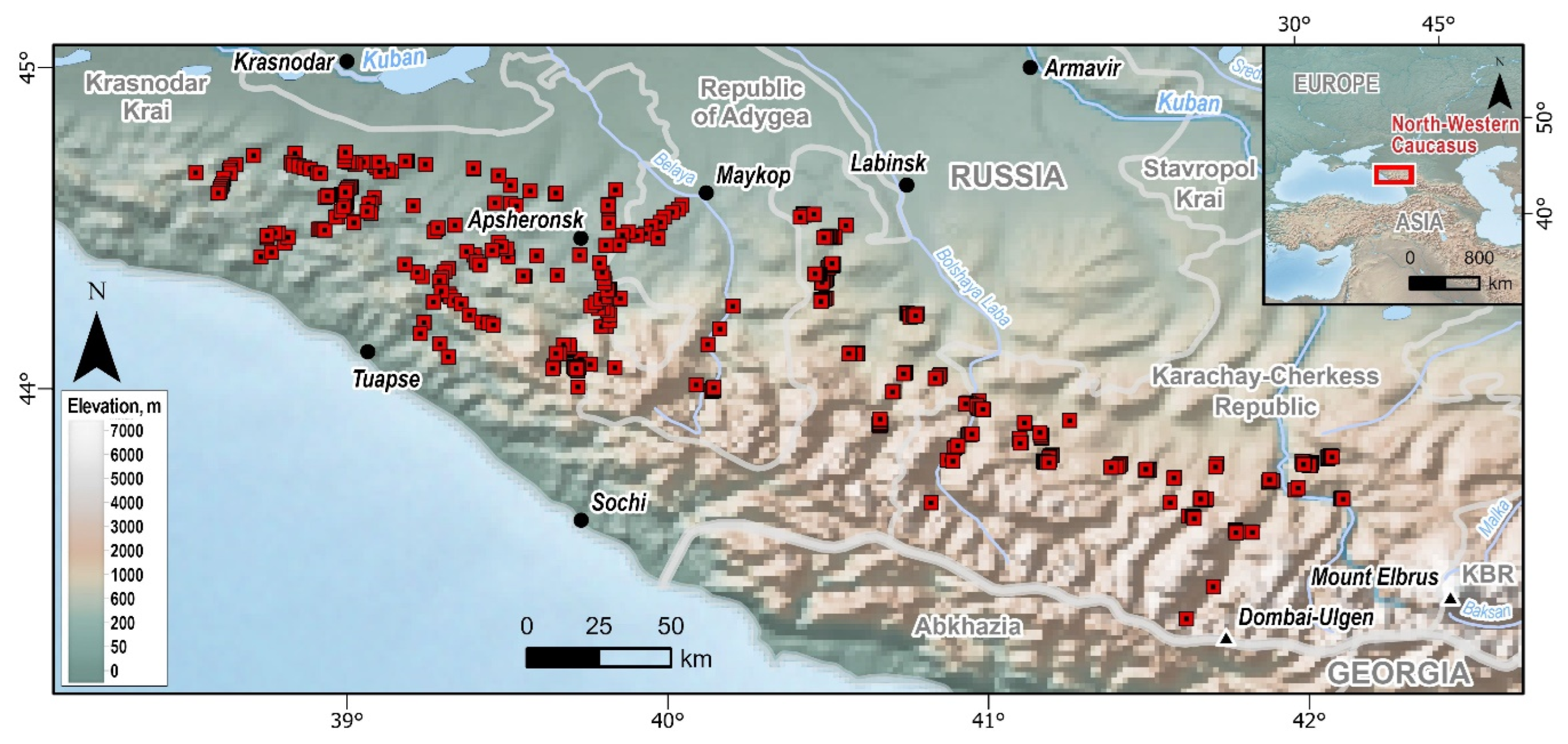
Figure 2.
The matrices of pairwise Jaccard index values between the floristic and the dominant classification: (a) Generalized classes; (b) Detailed classes. Classes’ designations are given according to Table 2 and Table 3.
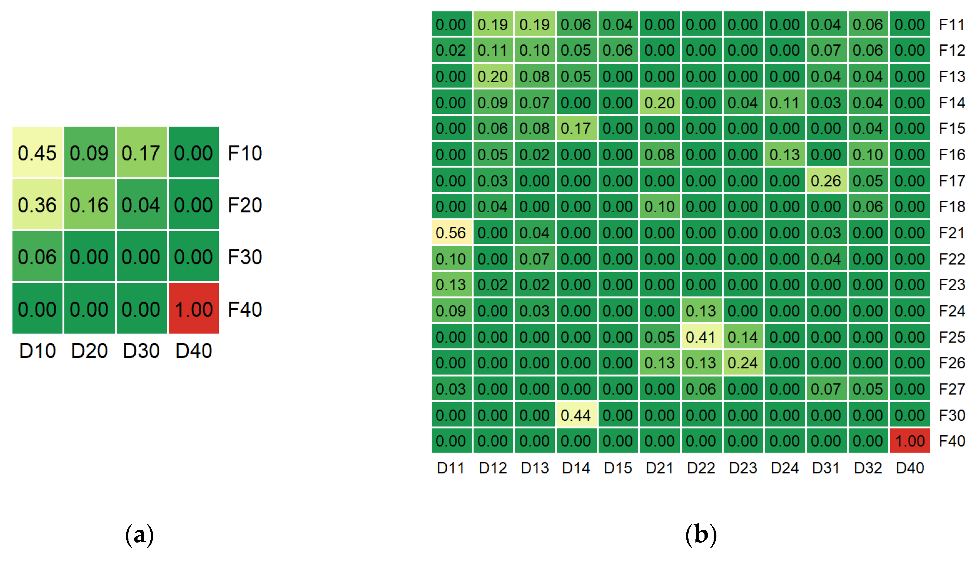
Figure 3.
Pairwise fractions of shared variables, selected for the different classification types, depending on the initial variable set: (a, e) All available variables; (b, f) Environmental variables; (c, g) High spatial resolution variables; (d, h) Optical satellite-based variables. The upper row (a, b, c, d) represents the results for the entire selected variable set, the lower row (e, f, g, h) – for the 5 topmost effective variables in every set. Classification types: FG – floristic generalized, FD – floristic detailed, DG – dominant generalized, DD – dominant detailed.
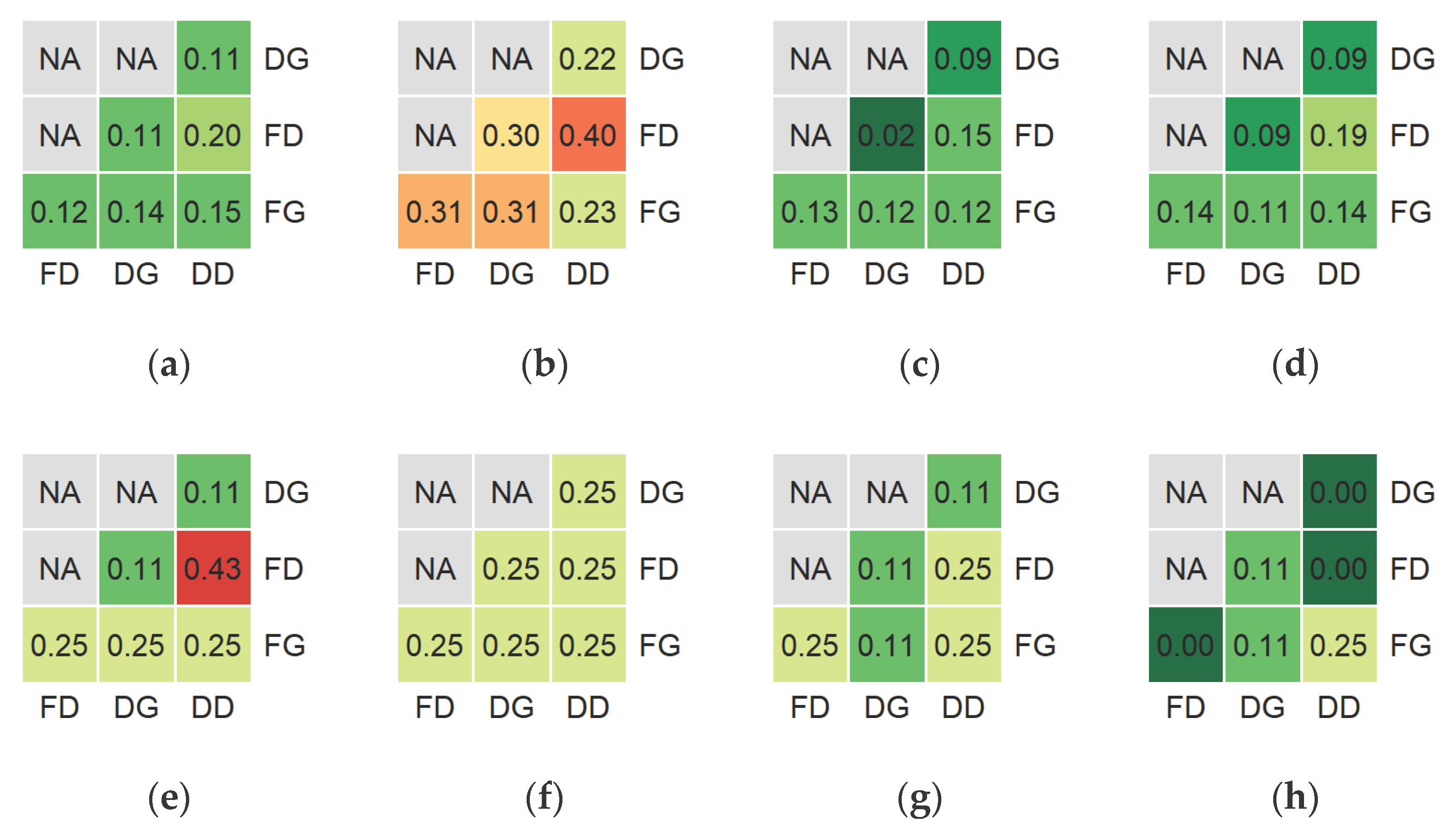

Table 1.
Reference fraction patterns for tree species groups and the respective generalized forest types for the dominant classification.
Table 1.
Reference fraction patterns for tree species groups and the respective generalized forest types for the dominant classification.
| Tree cover canopy fraction for groups of species: | Generalized forest type |
|||
|---|---|---|---|---|
| Dark coniferous |
Light coniferous |
Hard-leaved broadleaf |
Soft-leaved broadleaf |
|
| 1.0 | 0 | 0 | 0 | Dark coniferous |
| 0 | 1.0 | 0 | 0 | Light coniferous |
| 0 | 0 | 1.0 | 0 | Hard-leaved broadleaf |
| 0 | 0 | 0 | 1.0 | Soft-leaved broadleaf |
| 0.5 | 0.5 | 0 | 0 | Mixed coniferous |
| 0 | 0 | 0.5 | 0.5 | Mixed broadleaf |
| 0.5 | 0 | 0 | 0.5 | Mixed coniferous-broadleaf |
| 0 | 0.5 | 0.5 | 0 | |
| 0 | 0.5 | 0 | 0.5 | |
| 0.5 | 0 | 0.5 | 0 | |
| 0.33 | 0.33 | 0.33 | 0 | |
| 0.33 | 0.33 | 0 | 0.33 | |
| 0.33 | 0 | 0.33 | 0.33 | |
| 0 | 0.33 | 0.33 | 0.33 | |
| 0.25 | 0.25 | 0.25 | 0.25 | |
Table 2.
Floristic classification results.
| Class ID 1 | Reference Syntaxon name2 | Forest type | Sample size |
Sample fraction, % |
|
|---|---|---|---|---|---|
| FG | FD | ||||
| F10 | ord. Carpinetalia betuli (within: cl. Carpino-Fagetea) |
Hornbeam forests | 282 | 54.8 | |
| F11 | ass. Tamo communis–Carpinetum betuli var. typica |
Typical mesophytic hornbeam forests | 73 | 14.2 | |
| F12 | ass. Aro maculati–Carpinetum betuli | Hygromesophytic hornbeam forests | 48 | 9.3 | |
| F13 | ass. Tamo communis–Carpinetum betuli var. Staphylea colchica |
Thermophylized mesophytic hornbeam forests | 46 | 8.9 | |
| F14 | comm. Abies nordmannianae–Carpinus betulus var. typica |
Typical mesophytic beech forests with a little admixture of fir trees | 43 | 8.3 | |
| F15 | ass. Tamo communis–Carpinetum betuli var. Festuca drymeja |
Xeromesophytic hornbeam forests with a little admixture of sessile oak trees | 29 | 5.6 | |
| F16 | comm. Abies nordmannianae–Carpinus betulus var. Juncus effusus |
Semi-opened post-cut hygromesophytic hornbeam forests with admixture of quaking aspen & fir trees | 18 | 3.5 | |
| F17 | comm. Abies nordmannianae–Carpinus betulus var. Populus tremula |
Post-cut mesophytic hornbeam forests with an admixture of quaking aspen & fir trees | 16 | 3.1 | |
| F18 | ass. Dryopterido filicis-maris–Carpinetum betuli var. Alnus glutinosa |
Post-cut hygromesophytic hornbeam forests with admixture of black alder & fir trees | 9 | 1.7 | |
| F20 | ord. Rhododendro pontici–Fagetalia orientalis (within: cl. Carpino-Fagetea) |
Beech and conifer-beech forests | 196 | 38.1 | |
| F21 | ass. Myosotido amoenae–Fagetum orientalis subass. typicum |
Typical mesophytic beech forests | 90 | 17.5 | |
| F22 | ass. Aro maculati–Fagetum orientalis | Hygromesophytic beech forests | 24 | 4.7 | |
| F23 | ass. Lonicero caprifolii–Fagetum orientalis | Xeromesophytic beech forests | 22 | 4.3 | |
| F24 | ass. Myosotido amoenae–Fagetum orientalis subass. piceetosum orientalis |
Typical mesophytic beech forests with a little admixture of dark-conifer trees (fir, spruce) | 21 | 4.1 | |
| F25 | ass. Sambuco nigrae–Fagetum orientalis subass. typicum |
Typical mesophytic mixed fir & beech forests | 16 | 3.1 | |
| F26 | ass. Sambuco nigrae–Fagetum orientalis subass. typicum var. Rubus caesius |
Semi-opened hygromesophytic mixed fir & beech forests | 12 | 2.3 | |
| F27 | ass. Polygonato verticillati–Fagetum orientalis | Post-meadow mesophytic beech forests with a little admixture of pine, aspen, and birch trees | 11 | 2.1 | |
| F30 | ord. Quercetalia pubescenti-petraeae (within: cl. Quercetea pubescentis) |
Xerophytic open oak forests | 23 | 4.5 | |
| F30 | ass. Phleo phleoidis–Quercetum petraeae | Xerophytic sessile oak forests | 23 | 4.5 | |
| F40 | ord. Acero trautvetteri–Betuletalia litwinowii (within: cl. Betulo–Alnetea viridis) |
Subalpine open deciduous krummholz and scrub communities | 14 | 2.7 | |
| F40 | ass. Rhododendro caucasici–Betuletum litwinowii var. Calamagrostis arundinacea |
Subalpine open mesophytic birch forests | 14 | 2.7 | |
1 FG denotes the IDs for the generalized classification variant, FD – for the detailed one. 2 Complete syntaxon names are given in Table S2 of Supplementary Materials.
Table 3.
Dominant classification results.
| Class ID 1 | Forest type | Sample size |
Sample fraction, % |
|
|---|---|---|---|---|
| DG | DD | |||
| D10 | Hard-leaved broadleaf forests: | 379 | 73.6 | |
| D11 | with beech dominance | 135 | 26.2 | |
| D12 | with hornbeam dominance | 103 | 20 | |
| D13 | with mixed composition | 83 | 16.1 | |
| D14 | with oak dominance | 52 | 10.1 | |
| D15 | with ash dominance | 6 | 1.2 | |
| D20 | Mixed coniferous-broadleaf forests: | 62 | 12 | |
| D21 | with mixed composition | 23 | 4.5 | |
| D22 | with beech dominance | 22 | 4.3 | |
| D23 | with fir dominance | 9 | 1.7 | |
| D24 | with hornbeam dominance | 8 | 1.6 | |
| D30 | Mixed broadleaf forests: | 60 | 11.7 | |
| D31 | with hard-leaved dominance | 32 | 6.2 | |
| D32 | with soft-leaved dominance | 28 | 5.4 | |
| D40 | Soft-leaved broadleaf forests: | 14 | 2.7 | |
| D40 | with birch dominance | 14 | 2.7 | |
1 DG denotes the IDs for the generalized classification variant, DD – for the detailed one.
Table 4.
Aggregated feature selection results based on FOCI procedure.
| Classification type |
Initial variable set |
N | CODEC, % |
CODEC/N, % |
CODEC by variables’ type, % | |||
|---|---|---|---|---|---|---|---|---|
| Sat | DEM | WCB | Soil | |||||
| Floristic Generalized |
All | 9 | 86.4 | 9.6 | 2.3 | 2.1 | 77.5 | 4.5 |
| Env | 10 | 89.1 | 8.9 | – | 0.0 | 82.8 | 6.3 | |
| HiRes | 13 | 86.0 | 6.6 | 19.8 | 66.2 | – | – | |
| Sat | 19 | 86.9 | 4.6 | 86.9 | – | – | – | |
| Floristic Detailed |
Env | 28 | 66.7 | 2.4 | – | 2.2 | 42.2 | 22.4 |
| All | 48 | 71.2 | 1.5 | 15.1 | 2.2 | 29.3 | 24.6 | |
| HiRes | 67 | 71.5 | 1.1 | 53.0 | 18.5 | – | – | |
| Sat | 65 | 67.5 | 1.0 | 67.5 | – | – | – | |
| Dominant Generalized |
Env | 11 | 60.3 | 5.5 | – | 0.7 | 37.6 | 22.1 |
| All | 15 | 65.2 | 4.3 | 11.1 | 2.2 | 38.4 | 13.5 | |
| HiRes | 16 | 60.5 | 3.8 | 30.7 | 29.8 | – | – | |
| Sat | 21 | 67.4 | 3.2 | 67.4 | – | – | – | |
| Dominant Detailed |
Env | 28 | 53.8 | 1.9 | – | 1.6 | 31.0 | 21.2 |
| HiRes | 34 | 55.7 | 1.6 | 34.7 | 21.0 | – | – | |
| All | 37 | 59.7 | 1.6 | 16.1 | 2.8 | 32.1 | 8.8 | |
| Sat | 37 | 56.8 | 1.5 | 56.8 | – | – | – | |
Table designations: N – the number of selected features, CODEC – averaged cumulative value of the conditional dependence coefficient, Sat – optical satellite-based variables, DEM – DEM-based variables, WCB – WorldClim bioclimatic variables, Soil – SoilGrids variables, All – set of all available variables, Env – set of environmental variables, HiRes – set of high spatial resolution variables.
Table 5.
The top five most effective variables, selected from the all-available initial set for the different classification types.
Table 5.
The top five most effective variables, selected from the all-available initial set for the different classification types.
| Variable type |
Variable description |
CODEC, % | |||
|---|---|---|---|---|---|
| FG | FD | DG | DD | ||
| WCB | Temperature seasonality (standard deviation) | 2.2 | 12.0 | 37.6 | 4.5 |
| Soil | Cation exchange capacity in the 0-5 cm layer | 2.3 | 2.3 | 2.3 | 3.1 |
| WCB | Precipitation of the warmest quarter | 0.0 | 5.3 | 0.9 | 17.5 |
| WCB | Precipitation of the coldest quarter | 7.6 | 7.2 | 0.0 | 6.5 |
| WCB | Mean temperature of the wettest quarter | 38.0 | 1.3 | 0.0 | 0.0 |
| WCB | Mean of monthly temperature ranges (diurnal range) | 0.0 | 1.9 | 0.0 | 3.4 |
| Soil | Organic Carbon density in the 0-5 cm layer | 0.0 | 0.6 | 2.6 | 0.0 |
| WCB | Minimal temperature of the coldest month | 29.6 | 0.0 | 0.0 | 0.0 |
| Soil | Total Nitrogen content in the 15-30 cm layer | 0.0 | 0.0 | 7.6 | 0.0 |
| Sat | FPC7 of the NR between RE2 and RE3 spectral bands | 0.0 | 0.0 | 7.4 | 0.0 |
| Soil | Bulk density of the fine earth fraction in the 15-30 cm layer | 0.0 | 6.1 | 0.0 | 0.0 |
| Soil | Total Nitrogen content in the 0-5 cm layer | 0.0 | 5.8 | 0.0 | 0.0 |
| Sat | FPC4 of the Green spectral band | 0.0 | 0.0 | 0.0 | 4.0 |
Table designations: CODEC – averaged value of the conditional dependence coefficient by classification type (top 5 values are in bolds): FG – floristic generalized, FD – floristic detailed, DG – dominant generalized, DD – dominant detailed; WCB – WorldClim bioclimatic variables, Soil – SoilGrids variables, Sat – satellite-based variables, FPCn – n-th functional principal component, NR – normalized ratio, RE2, RE3 – 2nd and 3rd red-edge spectral bands. .
Table 6.
Aggregated performance metrics for the best obtained classification models.
| Classification type |
Variable set |
Best MLA |
MCC, % | Overall Accuracy, % | Balanced Accuracy, % | |||||||||
|---|---|---|---|---|---|---|---|---|---|---|---|---|---|---|
| min | mean | max | SD | min | mean | max | SD | min | mean | max | SD | |||
| Floristic Generalized |
All | RF | 74.4 | 84.4 | 96.6 | 7.7 | 83.5 | 90.9 | 98.1 | 4.8 | 81.1 | 91.4 | 99.1 | 5.7 |
| HiRes | RF | 68.6 | 83.8 | 94.7 | 9.3 | 81.6 | 90.6 | 97.1 | 5.7 | 63.7 | 87.4 | 97.7 | 10.1 | |
| Env | CB | 68.8 | 82.7 | 96.6 | 8.7 | 80.6 | 90.0 | 98.1 | 5.3 | 74.8 | 89.0 | 99.1 | 6.8 | |
| Sat | RF | 58.9 | 80.4 | 98.2 | 11.8 | 77.7 | 88.9 | 99.0 | 6.7 | 49.1 | 83.0 | 93.8 | 13.0 | |
| none | Ref | 0.0 | 0.0 | 0.0 | 0.0 | 53.4 | 54.8 | 55.3 | 0.9 | 25.0 | 25.0 | 25.0 | 0.0 | |
| Floristic Detailed |
All | CB | 35.8 | 52.8 | 71.5 | 9.5 | 40.8 | 56.2 | 73.8 | 9.1 | 46.1 | 58.0 | 72.9 | 6.5 |
| HiRes | CB | 35.3 | 50.4 | 62.7 | 7.6 | 39.8 | 54.5 | 66.0 | 7.3 | 40.5 | 51.4 | 60.8 | 4.9 | |
| Sat | CB | 36.9 | 48.9 | 68.0 | 8.9 | 42.7 | 53.3 | 70.9 | 8.2 | 41.2 | 50.3 | 64.0 | 5.6 | |
| Env | CB | 33.6 | 44.3 | 57.5 | 6.0 | 36.9 | 47.8 | 60.2 | 6.1 | 38.3 | 50.6 | 59.8 | 4.6 | |
| none | Ref | 0.0 | 0.0 | 0.0 | 0.0 | 17.5 | 17.5 | 17.5 | 0.0 | 5.9 | 5.9 | 5.9 | 0.0 | |
| Dominant Generalized |
All | RF | 53.2 | 59.9 | 66.6 | 2.7 | 78.6 | 83.4 | 86.4 | 1.9 | 63.1 | 72.6 | 78.7 | 4.0 |
| Env | RF | 51.4 | 58.3 | 70.9 | 4.4 | 73.8 | 81.3 | 86.4 | 2.5 | 66.7 | 76.4 | 85.8 | 5.6 | |
| HiRes | RF | 44.1 | 55.3 | 62.8 | 3.5 | 76.7 | 80.7 | 84.5 | 1.6 | 55.1 | 73.2 | 82.0 | 6.0 | |
| Sat | RF | 42.5 | 53.6 | 71.8 | 6.3 | 71.8 | 80.4 | 88.3 | 3.9 | 59.7 | 69.8 | 78.1 | 4.4 | |
| none | Ref | 0.0 | 0.0 | 0.0 | 0.0 | 72.8 | 73.6 | 74.8 | 1.1 | 25.0 | 25.0 | 25.0 | 0.0 | |
| Dominant Detailed |
HiRes | RF | 32.1 | 44.0 | 50.5 | 4.7 | 40.8 | 52.1 | 58.3 | 4.4 | 40.1 | 46.4 | 60.2 | 6.3 |
| All | RF | 33.3 | 43.9 | 52.3 | 4.6 | 41.7 | 51.9 | 59.2 | 4.3 | 35.8 | 47.2 | 61.4 | 6.2 | |
| Sat | RF | 31.8 | 42.7 | 53.1 | 4.8 | 41.7 | 51.1 | 60.2 | 4.3 | 33.6 | 43.3 | 55.5 | 3.3 | |
| Env | CB | 22.9 | 40.7 | 54.0 | 8.3 | 33.0 | 49.4 | 61.2 | 7.3 | 35.4 | 45.7 | 60.8 | 6.5 | |
| none | Ref | 0.0 | 0.0 | 0.0 | 0.0 | 26.2 | 26.2 | 26.2 | 0.0 | 8.3 | 8.3 | 8.3 | 0.0 | |
Table designations: Variable set – origin of the optimized variable subset used for the model training (bolds have the significantly higher MCC mean values toward the regulars), All – all available variables, HiRes – high spatial resolution variables, Env – environmental variables, Sat – optical satellite-based variables; Best MLA – machine learning algorithm provided the highest mean MCC value for the particular variable set (in bold, if the difference in MCC mean values toward all other algorithms was statistically significant), RF – Random Forest, CB – CatBoost, Ref – featureless reference model; min, mean, max, SD – minimum, mean, maximum and Standard Deviation values of performance metrics acquired across all CV-folds and repetitions.
Table 7.
Confusion matrix and related accuracy statistics for the Generalized Floristic classification model based on the filtered set of all available variables.
Table 7.
Confusion matrix and related accuracy statistics for the Generalized Floristic classification model based on the filtered set of all available variables.
| Class ID |
F10 | F20 | F30 | F40 | Sums | Accuracy metrics, % | ||||
|---|---|---|---|---|---|---|---|---|---|---|
| True | Predicted | Recall | Precision | F1 | MCC | |||||
| F10 | 256.6 | 17.8 | 6.7 | 1.0 | 282.0 | 277.7 | 91.0 | 92.4 | 91.7 | 81.8 |
| F20 | 17.0 | 178.4 | 0.0 | 0.6 | 196.0 | 196.2 | 91.0 | 91.0 | 91.0 | 85.4 |
| F30 | 4.1 | 0.0 | 18.9 | 0.0 | 23.0 | 25.6 | 82.2 | 74.0 | 77.9 | 76.9 |
| F40 | 0.0 | 0.0 | 0.0 | 14.0 | 14.0 | 15.6 | 100.0 | 89.7 | 94.6 | 94.6 |
Table 8.
Confusion matrix and related accuracy statistics for the Generalized Dominant classification model based on the filtered set of all available variables.
Table 8.
Confusion matrix and related accuracy statistics for the Generalized Dominant classification model based on the filtered set of all available variables.
| Class ID |
D10 | D20 | D30 | D40 | Sums | Accuracy metrics, % | ||||
|---|---|---|---|---|---|---|---|---|---|---|
| True | Predicted | Recall | Precision | F1 | MCC | |||||
| D10 | 350.7 | 11.8 | 15.6 | 1.0 | 379.0 | 399.0 | 92.5 | 87.9 | 90.1 | 60.1 |
| D20 | 5.6 | 50.9 | 4.7 | 0.9 | 62.0 | 66.0 | 82.1 | 77.2 | 79.6 | 76.7 |
| D30 | 42.1 | 3.1 | 14.9 | 0.0 | 60.0 | 35.2 | 24.8 | 42.4 | 31.3 | 25.9 |
| D40 | 0.8 | 0.3 | 0.0 | 13.0 | 14.0 | 14.9 | 92.9 | 87.3 | 90.0 | 89.7 |
Table 9.
Confusion matrix and related accuracy statistics for the Detailed Floristic classification model based on the filtered set of all available variables.
Table 9.
Confusion matrix and related accuracy statistics for the Detailed Floristic classification model based on the filtered set of all available variables.
| Class ID |
F11 | F12 | F13 | F14 | F15 | F16 | F17 | F18 | F21 | F22 | F23 | F24 | F25 | F26 | F27 | F30 | F40 | Sums | Accuracy metrics, % | ||||
|---|---|---|---|---|---|---|---|---|---|---|---|---|---|---|---|---|---|---|---|---|---|---|---|
| True | Predicted | Recall | Precision | F1 | MCC | ||||||||||||||||||
| F11 | 38.1 | 0.6 | 16.9 | 6.3 | 2.9 | 1.2 | 0.0 | 0.0 | 1.0 | 0.1 | 0.5 | 2.1 | 0.1 | 0.0 | 0.0 | 2.5 | 1.0 | 73.0 | 65.3 | 52.1 | 58.3 | 55.1 | 48.2 |
| F12 | 0.0 | 38.3 | 0.0 | 0.0 | 0.0 | 0.0 | 0.0 | 0.0 | 0.0 | 6.1 | 3.7 | 0.0 | 0.0 | 0.0 | 0.0 | 0.0 | 0.0 | 48.0 | 50.6 | 79.8 | 75.7 | 77.7 | 75.4 |
| F13 | 8.9 | 0.0 | 25.5 | 4.4 | 5.2 | 0.2 | 0.3 | 0.3 | 0.0 | 0.0 | 0.1 | 0.0 | 0.0 | 0.0 | 0.0 | 1.4 | 0.0 | 46.0 | 54.9 | 55.3 | 46.4 | 50.5 | 45.4 |
| F14 | 4.3 | 0.0 | 1.6 | 24.4 | 2.8 | 1.1 | 4.8 | 2.1 | 0.0 | 0.0 | 0.0 | 0.0 | 0.7 | 1.4 | 0.0 | 0.1 | 0.0 | 43.0 | 46.5 | 56.6 | 52.4 | 54.4 | 50.2 |
| F15 | 11.3 | 0.0 | 7.0 | 3.9 | 3.6 | 0.0 | 0.0 | 0.0 | 0.0 | 0.0 | 0.0 | 0.0 | 0.0 | 0.0 | 0.0 | 3.4 | 0.0 | 29.0 | 19.0 | 12.2 | 18.7 | 14.8 | 11.1 |
| F16 | 0.0 | 0.0 | 0.0 | 0.6 | 0.0 | 13.5 | 2.8 | 1.2 | 0.0 | 0.0 | 0.0 | 0.0 | 0.0 | 0.0 | 0.0 | 0.0 | 0.0 | 18.0 | 17.6 | 74.7 | 76.4 | 75.6 | 74.7 |
| F17 | 0.0 | 0.0 | 0.0 | 2.6 | 0.0 | 1.6 | 11.7 | 0.1 | 0.0 | 0.0 | 0.0 | 0.0 | 0.0 | 0.0 | 0.0 | 0.0 | 0.0 | 16.0 | 19.6 | 73.1 | 59.7 | 65.7 | 64.9 |
| F18 | 0.0 | 0.0 | 0.0 | 2.5 | 0.0 | 0.0 | 0.1 | 6.5 | 0.0 | 0.0 | 0.0 | 0.0 | 0.0 | 0.0 | 0.0 | 0.0 | 0.0 | 9.0 | 10.1 | 71.7 | 64.2 | 67.7 | 67.2 |
| F21 | 1.0 | 0.2 | 0.0 | 0.9 | 0.0 | 0.0 | 0.0 | 0.0 | 52.5 | 11.6 | 10.6 | 3.1 | 0.1 | 0.1 | 10.0 | 0.0 | 0.0 | 90.0 | 73.8 | 58.3 | 71.2 | 64.1 | 57.8 |
| F22 | 0.2 | 6.6 | 0.0 | 0.0 | 0.0 | 0.0 | 0.0 | 0.0 | 5.5 | 8.8 | 1.0 | 2.1 | 0.0 | 0.0 | 0.0 | 0.0 | 0.0 | 24.0 | 31.9 | 36.5 | 27.5 | 31.3 | 27.8 |
| F23 | 0.0 | 5.0 | 2.0 | 0.9 | 0.0 | 0.1 | 0.0 | 0.0 | 9.7 | 2.3 | 1.4 | 0.2 | 0.0 | 0.0 | 0.6 | 0.0 | 0.0 | 22.0 | 19.6 | 6.4 | 7.2 | 6.7 | 2.8 |
| F24 | 1.2 | 0.0 | 0.0 | 0.0 | 0.0 | 0.0 | 0.0 | 0.0 | 2.7 | 3.0 | 2.3 | 10.8 | 0.0 | 0.0 | 0.4 | 0.0 | 0.8 | 21.0 | 19.2 | 51.2 | 56.1 | 53.6 | 51.7 |
| F25 | 0.0 | 0.0 | 0.0 | 0.0 | 0.0 | 0.0 | 0.0 | 0.0 | 0.0 | 0.0 | 0.0 | 0.0 | 11.5 | 4.5 | 0.0 | 0.0 | 0.0 | 16.0 | 18.5 | 71.9 | 62.3 | 66.8 | 65.8 |
| F26 | 0.0 | 0.0 | 0.0 | 0.1 | 0.0 | 0.0 | 0.0 | 0.0 | 0.0 | 0.0 | 0.0 | 0.0 | 6.1 | 5.8 | 0.0 | 0.0 | 0.0 | 12.0 | 11.7 | 48.3 | 49.6 | 49.0 | 47.8 |
| F27 | 0.0 | 0.0 | 0.0 | 0.0 | 0.0 | 0.0 | 0.0 | 0.0 | 2.5 | 0.1 | 0.0 | 0.0 | 0.0 | 0.0 | 8.4 | 0.0 | 0.0 | 11.0 | 19.4 | 76.4 | 43.4 | 55.4 | 56.4 |
| F30 | 0.6 | 0.0 | 2.0 | 0.0 | 4.6 | 0.0 | 0.0 | 0.0 | 0.0 | 0.0 | 0.0 | 0.0 | 0.0 | 0.0 | 0.0 | 15.9 | 0.0 | 23.0 | 23.2 | 69.1 | 68.7 | 68.9 | 67.5 |
| F40 | 0.0 | 0.0 | 0.0 | 0.0 | 0.0 | 0.0 | 0.0 | 0.0 | 0.0 | 0.0 | 0.0 | 1.0 | 0.0 | 0.0 | 0.0 | 0.0 | 13.0 | 14.0 | 14.7 | 92.9 | 88.4 | 90.6 | 90.4 |
Table 10.
Confusion matrix and related accuracy statistics for the Detailed Dominant classification model based on the filtered set of all available variables.
Table 10.
Confusion matrix and related accuracy statistics for the Detailed Dominant classification model based on the filtered set of all available variables.
| Class ID |
D11 | D12 | D13 | D14 | D15 | D21 | D22 | D23 | D24 | D31 | D32 | D40 | Sums | Accuracy metrics, % | ||||
|---|---|---|---|---|---|---|---|---|---|---|---|---|---|---|---|---|---|---|
| True | Predicted | Recall | Precision | F1 | MCC | |||||||||||||
| D11 | 112.7 | 5.0 | 4.8 | 0.2 | 5.2 | 2.0 | 3.3 | 0.0 | 0.0 | 1.0 | 1.0 | 0.0 | 135.0 | 149.8 | 83.4 | 75.2 | 79.1 | 71.3 |
| D12 | 4.2 | 47.2 | 10.5 | 16.0 | 1.0 | 10.9 | 0.9 | 0.1 | 0.3 | 8.4 | 2.8 | 1.0 | 103.0 | 98.3 | 45.8 | 48.0 | 46.9 | 34.0 |
| D13 | 18.5 | 22.7 | 12.0 | 16.7 | 0.0 | 2.4 | 1.1 | 0.0 | 1.9 | 3.3 | 4.6 | 0.0 | 83.0 | 40.9 | 14.5 | 29.4 | 19.4 | 10.6 |
| D14 | 1.0 | 6.9 | 5.7 | 38.5 | 0.0 | 0.0 | 0.0 | 0.0 | 0.0 | 0.0 | 0.0 | 0.0 | 52.0 | 76.6 | 74.0 | 50.3 | 59.9 | 55.8 |
| D15 | 1.1 | 1.1 | 1.6 | 1.0 | 1.2 | 0.0 | 0.0 | 0.0 | 0.0 | 0.1 | 0.1 | 0.0 | 6.0 | 7.3 | 20.0 | 16.4 | 18.1 | 17.1 |
| D21 | 0.0 | 0.4 | 0.6 | 0.0 | 0.0 | 13.7 | 5.7 | 0.0 | 2.6 | 0.1 | 0.0 | 0.0 | 23.0 | 37.0 | 59.4 | 36.9 | 45.5 | 43.7 |
| D22 | 2.5 | 0.0 | 0.0 | 0.0 | 0.0 | 1.2 | 13.5 | 4.9 | 0.0 | 0.0 | 0.0 | 0.0 | 22.0 | 32.4 | 61.4 | 41.7 | 49.7 | 48.0 |
| D23 | 0.0 | 0.0 | 0.0 | 0.0 | 0.0 | 1.0 | 6.2 | 1.8 | 0.0 | 0.0 | 0.0 | 0.0 | 9.0 | 6.8 | 20.0 | 26.7 | 22.9 | 21.9 |
| D24 | 0.0 | 0.0 | 0.0 | 0.0 | 0.0 | 2.1 | 0.0 | 0.0 | 3.9 | 2.0 | 0.0 | 0.0 | 8.0 | 12.4 | 48.8 | 31.6 | 38.3 | 38.1 |
| D31 | 7.0 | 5.8 | 3.7 | 1.2 | 0.0 | 1.9 | 0.9 | 0.0 | 2.7 | 7.3 | 1.6 | 0.0 | 32.0 | 27.2 | 22.8 | 26.8 | 24.7 | 20.2 |
| D32 | 3.0 | 9.3 | 2.2 | 3.1 | 0.0 | 1.9 | 0.0 | 0.0 | 1.1 | 5.1 | 2.5 | 0.0 | 28.0 | 12.5 | 8.8 | 19.6 | 12.1 | 9.9 |
| D40 | 0.0 | 0.0 | 0.0 | 0.0 | 0.0 | 0.0 | 0.9 | 0.0 | 0.0 | 0.0 | 0.0 | 13.1 | 14.0 | 14.1 | 93.6 | 92.9 | 93.2 | 93.1 |
Disclaimer/Publisher’s Note: The statements, opinions and data contained in all publications are solely those of the individual author(s) and contributor(s) and not of MDPI and/or the editor(s). MDPI and/or the editor(s) disclaim responsibility for any injury to people or property resulting from any ideas, methods, instructions or products referred to in the content. |
© 2025 by the authors. Licensee MDPI, Basel, Switzerland. This article is an open access article distributed under the terms and conditions of the Creative Commons Attribution (CC BY) license (http://creativecommons.org/licenses/by/4.0/).
Copyright: This open access article is published under a Creative Commons CC BY 4.0 license, which permit the free download, distribution, and reuse, provided that the author and preprint are cited in any reuse.


