
Submitted:
04 October 2025
Posted:
08 October 2025
You are already at the latest version
Abstract
The airborne wind turbine (AWT) employs a flying energy conversion to harvest the stronger winds blowing at higher altitudes. This study presents an aeroelastic evaluation of AWT which carries a flying rotor installed inside a buoyant shell. A considerable aerodynamic impact on the structural integrity of the full-scale system is modeled using fluid–structure interaction (FSI) approach. Both the fluid model and structure model are formulated separately and validated by a series of benchmark numerical data. To analyze the structural aeroelasticity, the aerodynamic loads from the fully-resolved computational model are coupled using one-way FSI to the structural model of the blade and shell to perform the non-linear static analysis. For detailed investigation, various wind loads from the bare and shell rotor configurations are imposed on the flexible structure. The generated torque, aerodynamic loads, tip deflection, stress estimation and operational stability of the proposed energy system are computed. The nonlinear aeroelastic characteristics in each case are found to be within the chosen design criteria according to material, operational speed and structural limits. Most importantly, the significant power gain justifies the structural response of the blade to withstand the shell induced loads at rated conditions in the shell configuration.
Keywords:
aeroelastic modeling
; airborne wind turbine
; computational fluid dynamics
; aerodynamic and structural performance
; fluid–structure interaction
; finite element method
; renewable energy
1. Introduction
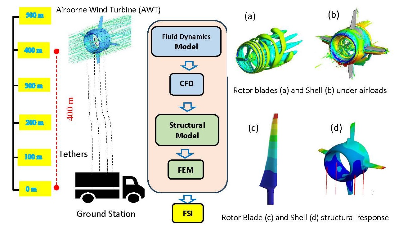
Since the last decade, new trends in the wind turbine industry have steadily grown with the objective of novel harvesting technologies in favor of renewable energies [1]. Especially the airborne wind energy systems (AWESs) [2] have many undeniable advantages over traditional wind turbines to capture untapped energy [3] referred to as airborne wind energy (AWE) [4] of atmosphere layers. On the other hand, tower-based wind turbines have limited potential to harness the consistent winds blowing at elevated heights [5] due to the high-rise buildings, tower constraints, uneven terrain [6] and meteorological conditions. Subsequently, a technique of buoyant airborne turbine (BAT) is introduced as a unique representative of the AWT. Technically, the hardware configuration of the BAT energy system consists of a small size of rotor placed inside a helium-filled buoyant shell [7] while the entire assembly is lifted to operate at 400 m height. Despite beneficial yield, the AWT often confronts the challenges of increased wind speeds that might result in aeroelastic instabilities [8] of the wind converter which can be devastating to the rotor blades. Hence, accurate FSI modeling is crucial to investigate the BAT energy system.
The aerodynamic behavior of the BAT can be characterized by the ducted wind turbine (DWT) [9,10] or diffuser augmented wind turbine (DAWT) [11,12]. In contrast to the solid duct in DWT, the BAT is equipped with a flexible buoyant shell. Consequently, the enclosed helium gas generates the aerostatic lift to raise the BAT system at desired altitudes. From a numerical point of view [13], many researchers opted to investigate the aerodynamic performance of the ducted or shell-based turbines using a numerical approach. Different studies were carried out to evaluate the DWTs by employing the blade element momentum (BEM) and computational fluid dynamics (CFD) numerical approaches [14]. The Reynolds-averaged Navier–Stokes (RANS) based CFD simulations were conducted while enclosing the rotor inside an airfoil-based shroud [15], duct [16] and stepped duct [17]. Likewise, in the BAT system, many authors incorporated the RANS-CFD approach for the evaluation of the aerodynamic performance of 2-bladed rotor [18,19] and 3-bladed rotor [20] in a buoyant shell configuration. However, the majority of these analyses focus on the aerodynamic aspect of the DWTs in terms of performance analysis. For this reason, in this present study, the CFD analysis together with finite element method (FEM) analysis [21] was performed to analyze the structural integrity of AWT through FSI analysis.
The applicability of FSI analysis that combines the fluid and structural modules to compute the power output, stresses, and deflection has been broadly discussed in the literature. From the FSI modeling perspective of the rotor [22], most researchers extensively applied the CFD and FEM techniques to measure the aeroelastic responses on horizontal axis wind turbines (HAWTs) [23] and NREL phase VI wind turbines [24]. Similarly, the elasto-flexible membrane blade [25], vertical axis wind turbines (VAWTs) [26] and floating offshore wind turbines [27] were also put forward for numerical analysis. A CFD study was conducted using 20 kW NREL wind turbine by implementing morphing features [28]. The reliability of 15MW blades rotor of HAWT was assessed through FSI Simulations by combining Kriging model and Monte Carlo simulation. The promising results of our study can be expand into the creation of digital twins for wind turbines [29]. The optimization of the structural topology of H-Rotor blade based on a one-way FSI approach by coupling URANS with density based topology optimization method. The blade mass can be easily reduced by around 60% with the devised approach [30]. The slender blades of a full-scale floating 15 MW wind turbine were analyzed by establishing CFD-FEA approach under wave-induced motions on the wind field [31]. A general FSI framework combining CFD, FEA and multi-body dynamics (MBD) was proposed to evaluate the detailed stress distributions on the composite structures of wind turbine blade [32].
The aeroelastic response of the NREL 5 MW wind turbine under diverse inflow conditions by integrating an improved actuator line model ALM with an equivalent beam model [33]. The dynamic response of the H-type floating VAWT platform was explored using the coupled CFD-FEM method [34]. At present, artificial intelligence (AI) [35] playing an important role in the design and optimization of offshore floating wind turbines [36]. A fully coupled aero-elastic-hydro-mooring framework by CFD and FEM, NREL 5 MW HAWT mounted on a semi-submersible platform, was investigated under combined wind and wave loading [36]. The ANSYS-based one-way FSI study was conducted to assess the blade lifespan of two small-scale wind turbines under different wind speeds [37]. Recently, a deep learning based framework that integrates CNN-BEM-FEM models to perform FSI analysis for a composite blade of a tidal turbine [38]. Two-way FSI for a 4.5 MW wind turbine was carried out by integrating the Large eddy simulation (LES) and structural dynamics to investigate the aeroelastic responses considering the flexibility of the blade and tower [39]. The simulated time series via BEM and CFD based modeling approaches can be incorporated with the data-driven approach of high fidelity aeroelastic analysis [40].
Most of these aeroelastic analyses generally provide reasonable results by taking into account the geometric nonlinearities to estimate the large blade deflections and blade-tower interaction. Despite the undertaken research, very limited literature is available regarding the FSI modeling of the ducted or shell turbine. There only a few attempts have been made to understand the FSI behavior of a buoyant shell [41] and ducted turbine [42]. Moreover, the available literature is incapable of providing detailed information regarding the aerodynamic and nonlinear structural design [43] of the rotor in ducted/shell configuration. Therefore, it is imperative to account for these research gaps and significantly contribute to a more detailed study to gain insight into the three-dimensional (3D) aeroelastic modeling of the AWT. Hence, a one-way FSI analysis that couples [44] the higher resolution methods of CFD and FEM is performed by investigating the structural behaviors [45] together with the safe functionality of the rotor. Most importantly, the characteristics of the analyzed problem are deeply examined with respect to the complex loading of the shell around the rotor blades.
The prime aim of this paper is to present a one-way FSI analysis for an airborne wind turbine at full scale. The task of a reliable aeroelastic model is accomplished by coupling the CFD and FEM models of the blade as well as the shell geometry. To maintain the proper stiffness, the blade is reinforced geometrically through a shear web. Similarly, the structural aspects of the shell’s deformable envelope are supposed to be a semi-rigid structure. Furthermore, the blade and shell were simplified by orthotropic and anisotropic material properties, respectively. The pressure loads in terms of fully converged steady-state are computed using CFD and then directly transferred to the structural surface. To determine the structural responses, nonlinear static structural analysis is performed using the developed FEM model. The main contribution is being made to enhance the clarity of the current study by explaining the rotor and shell models in parallel from CFD and FEM viewpoints throughout the paper. The results obtained using the one-way FSI approach are based on six operational conditions while the tip deformations and maximum stresses are found to be within structural limits. In addition, the numerical framework of the presented FSI model can be applied to many similar applications, such as ducted wind devices, a ducted propeller for urban air mobility and tidal turbines.
2. Bat Energy System
A 3-bladed upwind rotor consisting of the twisted and tapered shape of blades [46] was employed in a ring-shaped buoyant shell. The outer blade shape was composed of three different airfoils and was originally designed to operate at an airborne altitude of 400 m height. The radius of the rotor blade has span of 2.51 m that is a representative of a power output of 30kW under rated tip speed ratio (TSR) of 6.5. On the other hand, the outer aerodynamic shape of the shell [20] was modeled using a Delft University airfoil (DU 93-W-210). This airfoil was selected because of its characteristics of a moderate cambered of 2.85% and a maximum relative thickness of 21%. The main aim of the installation of the shell around the rotor blades is to provide beneficial velocity speed-up at the rotor plane. The major advantage of aerostatic lift comes from the buoyant force . This upward buoyancy force is generated from the helium gas enclosed inside the internal volume of the shell. The two main aerodynamic components of the BAT energy system i.e., rotor and shell are shown in Figure 1. The details of the geometric models will be discussed in subsection 4.1 whereas the specifications of the rotor and shell are outlined in Table 1.
3. One-Way FSI Analysis
The modeling framework of the fluid-structure interaction (FSI) analysis [47] is composed of the coupling of the fluid model (CFD model) and structural model (FEM model). There are two main approaches of coupling to solve the model for the FSI analysis, namely two-way coupling and one-way coupling. The two-way FSI is a direct coupling approach, the fluid model and structural model are solved simultaneously but separately to acquire and exchange the resulting data of pressure loads and displacement, respectively. On the other hand, in a one-way coupling model, the fully converged aerodynamic loads in the steady-state are obtained from CFD and are transferred to the FEM model to predict the response behavior of a single blade. The procedure is executed in such a way that the resulting displacement data is not mapped back to the fluid model. Furthermore, the one-way coupling is particularly suited for initial modeling purposes within a reasonable computing cost. For this reason, the one-way FSI coupling method is selected for aeroelastic modeling in this study as explained in Figure 2.
3.1. Fluid Model
The fluid model was developed using the ANSYS-CFX® software [48] to evaluate the CFD simulations. The CFD solver employs the finite volume method (FVM) approach for spatial discretization. The steady and incompressible RANS equations are incorporated to calculate the averaging flow quantities as wind loads on the resulting model. Mathematically, the governing equations of the mass and momentum are given as [49,50]:
Here the terms and denote the fluid density, pressure, dynamic viscosity and body force, respectively. The unknown term represents the Reynolds stress. To simulate turbulent flow, the shear stress transport (SST) model [51] was enabled at preprocessing level. The SST model was chosen because of its well-known capability in handling the external flows over the surface of wind turbines and wings [52]. The SST turbulence model is a two-equations model that expresses the two additional transport equations in the following form of Eq. (3) and Eq. (4):
The left-hand side of Eqs. (3) and (4) represent the change and transport of the turbulent kinetic energy and turbulent dissipation rate , respectively. Likewise, on the right-hand side of Eqs. (3) and (4) express the rate of production, turbulent diffusion, and rate of diffusion of k and ω, respectively. The term in Eq. (4) defines the blending function which acts as a switch for certain values between standard k–ε and k–ω turbulence models.
3.2. Structural Model
The FEM approach of the ANSYS static structural module [53] allows breaking the spatial domain of the model into quadrilaterals and triangle elements. The governing equation in static structural analysis () is expressed in differential form as conservation of momentum and is known as Cauchy’s equation of motion [54].
Here is the density, stands for the body force per unit mass in i-th direction, refers to the del, or nabla operator and is the Cauchy stress tensor. Hence, the partial differential expression of Cauchy’s equation that is governing the static equilibrium of the body takes the following forms:
Here the represents the body force per unit volume.With the assumption of large deformation, the strain-displacement relations reflect the following form of the compatibility equations [55]:
The stress and strain relationship of orthotropic material [56] can be described as a constitutive equation with respect to an orthonormal coordinate system. The symmetry transformations of orthotropic materials about all three orthogonal planes are as follows [57]:
Here is Young’s modulus in the i-th direction, is the shear modulus in ij plane, is the Poisson ratios.
4. Method of Solution
4.1. Geometric Models
The geometry of the rotor blade was modeled using the S-series of thick-airfoils family i.e., S-820, S-819 and S-821[58]. Similarly, the DU 93-W-210 airfoil and NACA-0012 airfoil were used to constitute the torus body of the shell and the projected wing, respectively. The geometric configuration, dimensions and shape of incorporated airfoils of the single blade and shell are shown in Figure 3. In view of the structural analysis, geometries were further segmented in multiple surfaces and a shear web was additionally introduced as illustrated in Figure 4 (a) and (b).
4.2. Mesh Models
For the fluid model in CFD analysis, a hexahedron mesh of high resolution was applied to constructed geometries based on 3D blocking topologies in ANSYS ICEM. First, the mesh generation of a single rotor was accomplished by adopting a C-type blocking topology. Second, the shell geometry was meshed using a series of O-grid topologies. The generated mesh of rotor and shell geometry is shown in Figure 5 (a) and (b). For the structural model in FEM analysis, a surface mesh of the rotor and shell was generated by a mean of 4-node shell-181 elements based on 2D blocking topologies illustrated in Figure 5 (c) and (d). To build a body-fitted mesh, a combination of quadrilateral and triangle cell shapes was incorporated within the ANSYS ICEM.
4.3. Boundary Conditions (BCs) and Domains
For the CFD model, the stationary domain was established to act as the outer fluid domain. The shell was modeled inside while the rotating domain carrying the mesh model of the rotor blades was placed inside the gap into . In steady-state analysis, a rotor blade with a faster simulation approach of Frozen Rotor was applied to impart the associated momentum terms into flow unlike the actuator disc approach where blade geometries need not be modeled. The non-conformal mesh connections were defined at overlapped interfaces. The domain sizes and boundary conditions (BCs) of the inlet and out are depicted in Figure 6 (a). The pressure loads obtained from the CFD analysis were then input into the static structural model to act as pressure BC. The other BCs input for the FEM software was the rotor’s rpm, fixed support at the root region and remote displacement (rigid support) for the shell geometry as shown in Figure 6 (b) and (c).
4.4. Shell Elements and Material Distribution
For model simplification, orthotropic and Kevlar-49 material properties based on the linear elastic model were selected to examine the rotor blade and shell in static structural analysis, respectively, as given in Table 2. Generally, the thin blades of wind turbines are produced with composite layups. The orthotropic material as a subset of composite material is primarily intended to reduce the material modeling efforts in structural analysis.
The selection of the shell-181 element is the most suitable choice when the thickness of the structure is significantly smaller than the other dimensions of the structure. The shell thickness of the blade is defined as sectional property and is calculated by the following relation [59].
In general, the direction of the x-axis of shell-181 is oriented by the nodal connectivity running from I-node to J-node (see Figure 7 (a)). Therefore, the element orientation was determined by using an orientation definition of the element coordinate system corresponding to the surface geometry of the blade as shown in Figure 7 (b). A varying thickness ranging from 5 mm (root) to 2 mm (tip) was used for the blade surface while a uniform thickness of 1 mm was used for the shell surfaces. Referring to Figure 8 (a), a familiar distribution of chord length and twist angle is gradually changing from the root to the tip region of the blade. A similar trend just like geometric entities can be observed in the case of material thickness and mass distribution as shown in Figure 8 (b).
4.5. Mesh Sensitivity Analysis
An assessment of the sensitivity of the mesh was performed for both the CFD and FEM models well before the FSI analysis. The CFD models of the blade and shell were analyzed at rated conditions using four sets of mesh models and performance parameters were monitored in each simulation. The gradual refinement of the mesh model from mesh 1 to mesh 4 permits the selection of the appropriate mesh density in terms of performance indicator and iteration time. Finally, mesh 3 was selected based on the percentage difference (between mesh 3 and mesh 4) of <1% and average time saving of >7% as described in Table 3.
For the mesh density of the FEM blade model, a modal analysis was performed on four different sets of meshes. The modal analysis is the fundamental dynamic analysis that provides the natural frequencies and mode shapes of the blade. In each set of meshes from mesh 1 to mesh 4, the FEM model was constrained at the root region of the blade and six modal frequencies (Hz) were calculated and compared as shown in Table 4. Based on the percentage difference, the FEM mesh model with 74,404 mesh elements was finally selected for further in-depth analysis of the non-linear static structural analysis of the blade. Likewise, several FEM meshes of different mesh densities for the buoyant shell were analyzed and a mesh with an element size of 1,46,130 was selected for further analysis. However, for brevity, the mesh sensitivity table of the shell is not included here.
5. Results and Discussion
5.1. Model Validation
The CFD model of the shell rotor must be verified to correctly determine the pressure load on the surface of rotor blades and buoyant shell. For model validation, the CFD model of the shell rotor was simulated at the rated wind speed () against varying TSRs ranging from . All the cases were run in steady-state flow for a minimum of 1200 iterations. The convergence criteria were set to to achieve a stable CFD solution. Next, the CFD model of the rotor in shell configuration was analyzed by processing the numerical data. The mechanical torque and thrust force acquired from the CFD model in shell configuration were used for the estimation of the total power output produced by the rotor. Similarly, the power coefficient of the shell rotor , the rotor thrust coefficient , rotor torque coefficient , can be calculated from the following relations:
Here the , and denotes the density of air at 400 m height, rated wind velocity and the blade radius, respectively. This extracted CFD data of various simulations were employed to generate curve. As the next step, curve of the fully resolved CFD model was compared with the ducted turbines available in the literature. Among the variety of ducted configurations, the chosen geometries of NACA-5415 (D1) [60], NACA-5415 (D2) [61] and DonQi [16] resembled more closely the shell’s shape of the current study.
Figure 9 displays a higher peak value of in the present study (DU-93-W-210) is 8% higher with respect to NACA-5415 (D1). Contrariwise, value is approximately 14% and 18 % less than those of NACA-5415 (D2) and DonQi ducted models. The discrepancies in model results are thought to be inherently associated with multiple factors that include the tip clearance, function of airfoil thickness and camber line, bending of the duct cross-section and numerical techniques. In fact, a scenario of different numerical techniques seems intuitive herein to explain the inconsistencies in the comparative analysis of the results because the performance of the rotor inside the DonQi duct was computed by the actuator disc model (ADM). Similarly, the NACA-5415 (D1) and NACA-5415 (D2) calculations were carried out via a semi-analytical method. In this regard, the ADM technique mimics the rotatory analysis of the rotor inside the duct through surface forces instead of actual blade geometry. The other notable limitations are evenly distributed rotor forces and the disregarded kinematics of the rotor’s wake.
The FEM model of the blade was validated with the model results calculated from the Numerical Manufacturing And Design (NuMAD) [62] tool. Basically, NuMAD is a quite user-friendly, stand-alone, MATLAB-based pre-processor for the FEM solver. First of all, the original blade model was replicated in the NuMAD graphics user environment. The material properties along with the desired design thickness were assigned to each blade section and shear web accordingly. As a further step, another program PreComp [63] was called to compute the stiffness and inertial properties of the blade at user-specified stations. PreComp calculates the detailed structural properties of the blade using an improved laminate theory.
For the calculation of the natural frequencies and mode shapes, the main output files of the PreComp were utilized as input files for another program BModes [64]. BModes takes the inputs in terms of the blade geometry, rotor speed and material distribution across the span of the blade. A salient feature of BModes is that it calculated the desired solution data by employing a cantilevered boundary condition at the blade root. However, the available version of BModes can only handle calculating the isotropic material properties of the structure instead. Hence, the modal analysis of the actual blade FEM model has been separately performed again with isotropic material properties to achieve comparable results in terms of modal parameters. For validation purposes, the natural frequencies of mode 1 and mode 2 obtained from both the solution solver are compared and found to be in close agreement as shown in Figure 10. The equation of FEM modal analysis is as follows;
Here and are the stiffness and mass matrices, respectively. Here, is called the angular frequency of a structure and are related to natural frequency in cycle per second (Hz) and represents the mode shape corresponds to certain .
5.2. Mode Shapes of Blade
Based on the modal characteristics [65], the free-vibration FEM procedure permits to evaluate the various mode shapes. A single FEM blade model rightly addresses the local solutions with non-rotating and fixed boundary conditions to the blade root. The first six vibration modes of the blade in flapwise and edgewise directions extracted from the FEM model are depicted in Figure 11 and Figure 12, respectively. As can be seen from mode shapes, the flapwise mode is dominating in the 1st, 3rd, 4th, 5th and 6th modes of free vibration. On the other hand, the edgewise mode is dominated by the 2nd mode and a slight glimpse appears in the 1st and 6th modes as well in Figure 12. These mode shape patterns are in line with the previous literature [23] which confirms the validity of the present FEM model.
5.3. Aerodynamic Forces and Augmentation
This section briefly describes the torque coefficient curves and the possible reasons behind the augmentation. Additionally, the aerodynamic forces on blade and shell structures are also discussed. An important curve of are replicated [20] here to illustrate the influence of wind speeds at a constant on the bare rotor and shell rotor as shown in Figure 13 (a). The predictions of rotor torque coefficient obtained from CFD indicates that the consistently raises with an increase in wind speed. As expected, the noticeable gain of ~66% higher torque coefficient is achieved with the same swept size of the rotor installed inside a shell under optimal conditions. The difference between the two examined configurations is quite profound at every given wind speed . This the increment can be further associated with mass swallowed by the rotor plane enclosed in the shell configuration. Figure 13 (b) shows the mass flow rate with varying values.
Despite the velocity disturbance at the rotor plane, using the ANSYS CFX built-in function accurately calculates the mass flow rate while accounting for these flow variations. This automatically integrates the local conditions over the specified surface, regardless of any disturbances caused by the rotor. One can notice a higher in case of shell rotor than that of the bare rotor under rated conditions. It can be easily seen that increases quite significantly with an increase in the given wind speed at constant TSR. This resulting increase in is mainly associated with shell geometry around rotor blades. Meanwhile, also holds a directly proportional relation with the wind speed .
An in-depth explanation requires the local velocity and pressure distributions. Figure 14 (a) presents a contour map of the normalized velocity in the yz-plane on a cross-section of the shell boundary. Under optimal conditions, the acceleration of airflow is less visible than the rotor tip. However, the relative magnitude of velocity appears to be comparatively high in the throat area and diminishes at the trailing edge. The disruptive action of the expansion ratio in the divergent section slows down the axial component further downstream of the rotor. (b) demonstrates the significant effect of the normalized pressure on the shell. In this pressure contour, the magnitude of the normalized pressure is considerably high at stagnation points such as the leading edge of the shell’s profile and stabilizing wing. High pressure is evident in the entire frontal portion of the shell. Herein, it is reasonable to summarize that the converged section largely causes a faster movement of the flow. Meanwhile, abrupt changes that occur in a narrow and diverged section indicate a larger diffusion of momentum, eddying flows and pressure recovery.
and corresponding mass flow rate .
To quantify the impact of tangential and normal forces with respect to the rotor blade, the rotor torque coefficient and rotor thrust coefficient , are drawn across the blade span as shown in Figure 15 (a) and (b). The distribution of both and of a single blade exhibits a quite similar behavior that tends to rise at the inboard region and then continues to increase gradually between . After that the maximum value of and approximately happens to appear in the outboard region and finally diminishes afterward in both configurations. Overall, higher aerodynamic forces in terms of and are achieved in the shell rotor compared to the bare rotor comes. Aerodynamically, the axial force experienced by the shell meaningfully contributes to the generate a higher thrust force in the case of the shell rotor. For this reason, a glimpse of the aerodynamic loadings on the shell is presented in terms of axial , tangential and normal forces at the three different spans (08%, 50%, and 85%) of the shell as shown in Figure 16. It can be seen that notable transition occurs in all loadings at an angular position of 90°, 180°, 270° and 0°/360° because of the shadow effects of the four stabilizing wings at these locations.
and thrust coefficients in bare and shell rotors.
5.4. Aeroelastic Structural Responses
The blade total deformations under three operational conditions of bare configuration and three operational conditions of shell configuration are depicted in Figure 17 (a)–(f). One can clearly observe that all the maximum deformations occur on the blade tip region for all operational conditions regardless of the type of configuration. This is also evidently visible that the blade-tip deflection consistently increases as the wind speed increases from to However, the tip deflection is considerably higher in order of magnitude under the shell configuration than that of the bare configuration. There are obvious results that stem from the fact that the rotor in the shell configuration experiences higher wind loads due to the flow augmentation effect of the shell structure around the rotor plane. It is therefore intuitive that the accelerated flow owing to the shell configuration is inherently associated with the increasing deflection on the rotor blade. Hence, relatively increased loads on the blade surface are supported by the higher power-producing cycle of the rotor in the shell configuration. For more clarity, the results can be described as percentages to further support the discussion related to tip deflection.
It is evident that when wind speed increases from 14–18 m/s the percentage increase in deflection is around 45% in the bare rotor configuration. This further increases and approaches 51% when wind speed shifts from 18 m/s to 22 m/s. This means that the tip deflection increased on an average of 47% corresponding to each time increase of 4 m/s in the free stream wind velocity. A similar trend is quite dominating in the shell configuration where 61% and 56% increase in deflection occur in 14–18 m/s and 18–22 m/s, respectively. On the other hand, when comparing the deflection of both the rotor configurations against each other few more aspects of the structural simulation can be uncovered. In the operational condition of 14 m/s, the deflection remains just below 6% in the shell configuration. However, the rated operational condition of 18 m/s approximately exhibits an 18% increase in tip deflection. Similarly, an increase of 21% is observed on the blade tip at higher wind loads of 22 m/s of the proposed airborne wind energy system. The observed increase in deformation with rising aerodynamic forces, despite the absence of a direct relationship, can be attributed to the complex, nonlinear response of rotor blades to wind loads. This complex interaction between aerodynamic loading, material response, rotational inertia, and geometric irregularities introduce fluctuating loads that further intensify these deformation effects.
Figure 18 shows the blade stress analysis of both the bare and shell configurations. The magnitude of the maximum stress was calculated normal to all three x-axis, y-axis and z-axis directions corresponding to and . The stress value is almost similar in both configurations in the x-axis at 14 m/s. One can visually see the stress magnitude is considerably high (>150%) in the z-axis direction in all cases of wind velocities. On the other hand, the equivalent stress exhibits a value very close to the z-axis stress magnitude since the z-axis direction contributed a much higher percentage than those of the other two axes. The profound effect of the stress concentration on the z-axis (flapwise deflection) is owing to the axial velocity in the z-direction during all the aerodynamic simulations. By considering the individual configuration, the stress increment is identified on an average of >45% and >55% corresponds to the bare and shell configuration.
Overall, the equivalent stress distribution on the rotor blade in shell configuration increases in all three cases of wind velocity 14 m/s, 18 m/s and 22 m/s up to 5%, 17% and 20%, respectively. In the worst case with a wind speed of 40 m/s, the maximum stress would reach by doubling the maximum stress values at 22 m/s on approximately 325 MPa based on linear relation. On the other hand, the tensile strength of most of the reinforced polymer composites ranges from 1000–2400 MPa. Generally, the material safety factor for wind turbine composite blades is around 2.2. In this case, the material safety factor is about 3.07, which is higher than the traditional benchmark of 2.2. This indicates the blade is unlikely to experience material failure under the given operational conditions.
As mentioned earlier, the goal of introducing a single shear web was to enhance the representative loads carrying capability of the blade. Figure 19 displays the stresses and strain induced in the shear web under wind loads of . The normalized values of stress and strain are drawn to determine how internal response could be mapped spanwise in the shell and bare rotor. The equivalent strain in terms of normal and shear stress components is estimated using the following relations;
Likewise, the von Mises stress or equivalent stress is written as:
The stress and strain data obtained from Eqs. (22) and (23) are then normalized by dividing the maximum value of the stress and strain data and plotted against the spanwise length of the shear web. The curves of stress and strain in each configuration are visually identical but differ in terms of the observed peak. The predicted values of stress and strain on the normalized numerical scale exhibit an increment of 17% and 20% in the shell rotor as compared to the bare rotor, respectively. The maximum value of stress and strain occurs about 0.4 span of the shear web. Considering the importance of region of this peak value, the outer shape of the blade has already been designed by employing an S-821 airfoil having a thickness of . The mounting evidence of structural analysis clearly justifies the use of a thick family of airfoils in modeling the blade. Additionally, the positioning of the S-821 airfoil was originally designed to facilitate the structural strength at the root region of the blade.
5.5. Operational Stability
Figure 20 shows the Campbell diagram of the blade model plotted from the initial modal analysis. A typical Campbell diagram provides an overall view of the vibration excitation that can occur on a rotating component during routine operation. The rotor blade was fixed at the root region while rotational velocity was applied clockwise in tabular form with an interval of 100 rpm having zero initial velocity. The first ten-mode shapes were subjected to generate the diagram in free vibration analysis. The natural frequencies of the system are plotted along the y-axis and the rotational velocity of the rotor on the x-axis. To meet structural and aerodynamic criteria, this frequency band indicates that operating the turbine above 611 rpm (red triangle) should be prohibited in all cases. It is pertinent to mention here that the design or rated operational speed of the rotor is 446 rpm and it is way below the computed threshold of the prohibited speed. In the worst-case scenario, the one possible situation the rotor blade might encounter is when it tends to achieve the TSR of 9.5 corresponding to the rotational velocity of 651 rpm at a rated wind speed of 18 m/s. However, it is already known from the aerodynamic analysis that the rotor must rotate near to rated rpm to optimize the power-producing cycle which restricts to avoid blade failure. Furthermore, the working operation of the rotor is reasonably stable in all the given rotational speeds other than that of the higher TSR close to the critical speed.
5.6. Deformation of Shell
To predict the deformation on the surface of the shell, the pressure loads were imported from the CFD solver at various load conditions. The pressure data from the CFD was perfectly mapped on the shell main as well as the four projected wings. These FEM simulations for the non-linear static structural analysis of the shell were simulated separately other than the rotor blades. For structural analysis of the shell, the sufficient deformation capacity of lower regions of the shell corresponding to the tethers joint must be ensured. Efforts were being made to model the tether’s effects through rigid support links to represent a physical consistent behavior of the shell structure. The simulations were carried out at three wind speeds of , and while the results of the total deformation can be seen in Figure 21 (a), (b) and (c). A relatively less deformation appears at the bottom half of the shell where the shell is constrained at four points using remote displacement boundary conditions. It is also visible that most of the deformation appears on the upper half of the shell.
The increment of wind velocity of from to shows a percentage change of 37% in deformation. On the other hand, when velocity changes from to a percentage change of about 20.4% is observed. Hence, the structural elements by carrying both the membrane stiffness and bending stiffness, the shell structure can be considered equivalent to the semi-rigid structure. Keeping in view the deformation of the shell, the rotor was purposefully placed with a tip clearance of around 590 mm (0.59 m) from the main body of the shell as shown in Figure 21 (d). In this perspective, the calculated deformation is quite reasonable that further ensures the smooth and safe working of the rotor inside the shell. From a static structural analysis viewpoint, the results are quite realistic with the underlying assumptions of the rigid tethers and semi-rigid structure of the shell.
6. Conclusions
The current study has been carried out to analyze the aeroelastic response of the airborne wind turbine (AWT). Two vital components of the AWT namely the rotor and shell have been studied through an approach based on the one-way fluid-structure interaction (FSI) analysis. The fluid model was first established to apply a range of wind loads which was undertaken for each simulation case using a fully-resolved CFD model. These wind loads in terms of CFD pressure load are transferred to the FEM model to predict the response behavior of the AWT for airborne applications. The blade and shell under augmented loads were further investigated for non-linearities that could indicate structural deformations and stresses. The important conclusions are listed below.
- The augmentation effects of the shell around the rotor yielded a substantial gain of 66% in generated torque as compared to the bare rotor. Conversely, the impact of the shell exerted a higher aerodynamic force on the rotor blades in the shell configuration. Thus, a trade-off between performance enhancement and the structural integrity of AWT is mandatory while operating at a high altitude.
- The blade structure reinforced by a shear web showed larger tip deflections (18% increment) in shell configuration than that of the bare rotor under rated conditions. This implies that the maximum tip deflection (~ 32 mm) at a rated wind speed of , indicating that the blade is least vulnerable to experience a strike with the surrounding structure. The results further revealed that the tip deflection increased by an average of 47% corresponding to an increment of 4 m/s in the wind speed.
- The maximum stresses built in the orthotropic blade were examined to be 160 MPa, which are well below the material strength limits of the composite. Additionally, there was no discernible material failure observed during non-linear static structural analysis. The rotational speed of the rotor was found to be quite stable and reasonably safe at a rated condition of 446 rpm.
- The predicted result of the FEM of the shell also ensured the functional operability of the rotor within the design requirement by indicating a limited deformation (~ 22 mm) of the shell surface. Overall the one-way FSI analysis is the preferable choice to evaluate the aerodynamic loads and non-linear structural responses using a dedicated CFD module coupled with the FEM module.
The present study fully focused on the aeroelastic responses for the design solution of an airborne wind energy harvester to operate at higher altitudes. An interesting line of future research would be to employ more realistic features on the rotor and shell by taking into account composite layups and membrane elements using a two-way FSI approach.
Author Contributions
Conceptualization, writing—original draft preparation, review and editing, Q.S.A. and M.-H.K.; methodology, software, validation, formal analysis, investigation, data curation, Q.S.A.; resources, supervision, project administration, funding acquisition, M.-H.K.; All authors have read and agreed to the published version of the manuscript.
Funding
This work was partly supported by the Korea Planning and Evaluation Institute of Industrial Technology (KEIT) grant funded by the Korea government (MOTIE) (Project number: RS-2024-00507617).
Data Availability Statement
Dataset available on request from the authors.
Conflicts of Interest
The authors declare no conflicts of interest.
Nomenclature
| shell exit area [ | ||
| shell area at rotor plane [ | ||
| power coefficient of shell rotor | ||
| power coefficient | ||
| thrust coefficient of rotor | ||
| torque coefficient of rotor | ||
| Young’s modulus | ||
| thrust force | ||
| axial force | ||
| force of buoyancy | ||
| normal force | ||
| tangential force | ||
| shear modulus | ||
| number of blades | ||
| rates power | ||
| total generated power | ||
| blade radius | ||
| mechanical torque | ||
| rated wind speed | ||
| chord length | ||
| natural frequency | ||
| mass flow rate | ||
| mass per unit length | ||
| thickness of shell-181 element | ||
| inner rotating domain | ||
| outer stationary domain | ||
| equivalent strain | ||
| rated tip speed ratio | ||
| Poisson’s ratio | ||
| air density at high altitudes | ||
| equivalent stress | ||
| altitude | ||
| wind speed | ||
| local radius | ||
| twist angle | ||
| azimuth rotation | ||
| tip speed ratio | ||
| density | ||
| angular speed | ||
| Stress | ||
| Young modulus | ||
| Strain | ||
| Cauchy stress tensor | ||
| Body force | ||
| Dispalcement | ||
| Shear modulus | ||
| Abbreviations | ||
| 2D | Two-dimensional | |
| 3D | Three-dimensional | |
| AWE | Airborne Wind Energy | |
| AWES | Airborne Wind Energy System | |
| AWT | Airborne Wind Turbine | |
| BAT | Buoyant Airborne Turbine | |
| BC | Boundary Condition | |
| BEM | Blade Element Momentum (model/theory) | |
| CFD | Computational Fluid Dynamics | |
| DAWT | Diffuser Augmented Wind Turbine | |
| DU | Delft University | |
| DWT | Ducted Wind Turbine | |
| FEM | Finite Element Method | |
| FoS | Factor of Safety | |
| FSI | Fluid–Structure Interaction | |
| FVM | Finite Volume Method | |
| HAWT | Horizontal Axis Wind Turbine | |
| NACA | National Advisory Committee for Aeronautics | |
| NREL | National Renewable Energy Laboratory | |
| NuMAD | Numerical Manufacturing And Design | |
| RANS | Reynolds-averaged Navier–Stokes (equations) | |
| rpm | Revolutions per Minute | |
| SST | Shear Stress Transport | |
| TSR | Tip Speed Ratio | |
| VAWT | Vertical Axis Wind Turbine | |
References
- Watson, S.; Moro, A.; Reis, V.; Baniotopoulos, C.; Barth, S.; Bartoli, G.; Bauer, F.; Boelman, E.; Bosse, D.; Cherubini, A.; et al. Future Emerging Technologies in the Wind Power Sector: A European Perspective. Renewable and Sustainable Energy Reviews 2019, 113, 109270. [CrossRef]
- Cherubini, A.; Papini, A.; Vertechy, R.; Fontana, M. Airborne Wind Energy Systems: A Review of the Technologies. Renewable and Sustainable Energy Reviews 2015, 51, 1461–1476. [CrossRef]
- Bechtle, P.; Schelbergen, M.; Schmehl, R.; Zillmann, U.; Watson, S. Airborne Wind Energy Resource Analysis. Renew Energy 2019, 141, 1103–1116. [CrossRef]
- Archer, C.L.; Delle Monache, L.; Rife, D.L. Airborne Wind Energy: Optimal Locations and Variability. Renew Energy 2014, 64, 180–186. [CrossRef]
- Archer, C.L.; Caldeira, K. Global Assessment of High-Altitude Wind Power. Energies (Basel) 2009, 2, 307–319. [CrossRef]
- Bansal, R.C.; Bhatti, T.S.; Kothari, D.P. On Some of the Design Aspects of Wind Energy Conversion Systems. Energy Convers Manag 2002, 43, 2175–2187. [CrossRef]
- Benjamin W. Glass US Patent for Lighter-Than-Aircraft for Energy Producing Turbines (Patent No. US 9000605 B2) 2015, 2, 22.
- Hansen, M.O.L.; Sørensen, J.N.; Voutsinas, S.; Sørensen, N.; Madsen, H.A. State of the Art in Wind Turbine Aerodynamics and Aeroelasticity. Progress in Aerospace Sciences 2006, 42, 285–330. [CrossRef]
- Saleem, A.; Kim, M.H. Effect of Rotor Tip Clearance on the Aerodynamic Performance of an Aerofoil-Based Ducted Wind Turbine. Energy Convers Manag 2019, 201, 112186. [CrossRef]
- Khamlaj, T.A.; Rumpfkeil, M.P. Analysis and Optimization of Ducted Wind Turbines. Energy 2018, 162, 1234–1252. [CrossRef]
- Liu, Y.; Yoshida, S. An Extension of the Generalized Actuator Disc Theory for Aerodynamic Analysis of the Diffuser-Augmented Wind Turbines. Energy 2015, 93, 1852–1859. [CrossRef]
- Hansen, M.O.L.; Sørensen, N.N.; Flay, R.G.J. Effect of Placing a Diffuser around a Wind Turbine. Wind Energy 2000, 3, 207–213. [CrossRef]
- Ahmed, M.R.; El Damatty, A.A.; Dai, K.; Ibrahim, A.; Lu, W. Parametric Study of the Quasi-Static Response of Wind Turbines in Downburst Conditions Using a Numerical Model. Eng Struct 2022, 250, 113440. [CrossRef]
- Bai, C.J.; Chen, P.W.; Wang, W.C. Aerodynamic Design and Analysis of a 10 KW Horizontal-Axis Wind Turbine for Tainan, Taiwan. Clean Technol Environ Policy 2016, 18, 1151–1166. [CrossRef]
- Aranake, A.C.; Lakshminarayan, V.K.; Duraisamy, K. Computational Analysis of Shrouded Wind Turbine Configurations Using a 3-Dimensional RANS Solver. Renew Energy 2015, 75, 818–832. [CrossRef]
- Dighe, V. V.; de Oliveira, G.; Avallone, F.; van Bussel, G.J.W. Characterization of Aerodynamic Performance of Ducted Wind Turbines: A Numerical Study. Wind Energy 2019, 22, 1655–1666. [CrossRef]
- Jafari, S.A.H.; Kosasih, B. Flow Analysis of Shrouded Small Wind Turbine with a Simple Frustum Diffuser with Computational Fluid Dynamics Simulations. Journal of Wind Engineering and Industrial Aerodynamics 2014, 125, 102–110. [CrossRef]
- Saeed, M.; Kim, M.H. Aerodynamic Performance Analysis of an Airborne Wind Turbine System with NREL Phase IV Rotor. Energy Convers Manag 2017, 134, 278–289. [CrossRef]
- Saleem, A.; Kim, M.H. Aerodynamic Analysis of an Airborne Wind Turbine with Three Different Aerofoil-Based Buoyant Shells Using Steady RANS Simulations. Energy Convers Manag 2018, 177, 233–248. [CrossRef]
- Ali, Q.S.; Kim, M. Quantifying Impacts of Shell Augmentation on Power Output of Airborne Wind Energy System at Elevated Heights. Energy 2022, 239, 121839. [CrossRef]
- Ali, A.; De Risi, R.; Sextos, A. Finite Element Modeling Optimization of Wind Turbine Blades from an Earthquake Engineering Perspective. Eng Struct 2020, 222, 111105. [CrossRef]
- Santo, G.; Peeters, M.; Van Paepegem, W.; Degroote, J. Effect of Rotor–Tower Interaction, Tilt Angle, and Yaw Misalignment on the Aeroelasticity of a Large Horizontal Axis Wind Turbine with Composite Blades. Wind Energy 2020, 23, 1578–1595. [CrossRef]
- Wang, L.; Quant, R.; Kolios, A. Fluid Structure Interaction Modelling of Horizontal-Axis Wind Turbine Blades Based on CFD and FEA. Journal of Wind Engineering and Industrial Aerodynamics 2016, 158, 11–25. [CrossRef]
- Lee, K.; Huque, Z.; Kommalapati, R.; Han, S.E. Fluid-Structure Interaction Analysis of NREL Phase VI Wind Turbine: Aerodynamic Force Evaluation and Structural Analysis Using FSI Analysis. Renew Energy 2017, 113, 512–531. [CrossRef]
- López, I.; Piquee, J.; Bucher, P.; Bletzinger, K.U.; Breitsamter, C.; Wüchner, R. Numerical Analysis of an Elasto-Flexible Membrane Blade Using Steady-State Fluid–Structure Interaction Simulations. J Fluids Struct 2021, 106, 103355. [CrossRef]
- Marzec, Ł.; Buliński, Z.; Krysiński, T. Fluid Structure Interaction Analysis of the Operating Savonius Wind Turbine. Renew Energy 2021, 164, 272–284. [CrossRef]
- Rodriguez, S.N.; Jaworski, J.W. Strongly-Coupled Aeroelastic Free-Vortex Wake Framework for Floating Offshore Wind Turbine Rotors. Part 2: Application. Renew Energy 2020, 149, 1018–1031. [CrossRef]
- Nejadkhaki, H.K.; Sohrabi, A.; Purandare, T.P.; Battaglia, F.; Hall, J.F. A Variable Twist Blade for Horizontal Axis Wind Turbines: Modeling and Analysis. Energy Convers Manag 2021, 248, 114771. [CrossRef]
- Keprate, A.; Bagalkot, N.; Siddiqui, M.S.; Sen, S. Reliability Analysis of 15MW Horizontal Axis Wind Turbine Rotor Blades Using Fluid-Structure Interaction Simulation and Adaptive Kriging Model. Ocean Engineering 2023, 288, 116138. [CrossRef]
- Marzec, L.; Buliński, Z.; Krysiński, T.; Tumidajski, J. Structural Optimisation of H-Rotor Wind Turbine Blade Based on One-Way Fluid Structure Interaction Approach. Renew Energy 2023, 216, 118957. [CrossRef]
- Zhang, D.; Liu, Z.; Li, W.; Zhang, J.; Cheng, L.; Hu, G. Fluid-Structure Interaction Analysis of Wind Turbine Aerodynamic Loads and Aeroelastic Responses Considering Blade and Tower Flexibility. Eng Struct 2024, 301, 117289. [CrossRef]
- Deng, Z.S.; Xiao, Q.; Huang, Y.; Yang, L.; Liu, Y.C. A General FSI Framework for an Effective Stress Analysis on Composite Wind Turbine Blades. Ocean Engineering 2024, 291, 116412. [CrossRef]
- Huang, Y.; Yang, X.; Zhao, W.; Wan, D. Aeroelastic Analysis of Wind Turbine under Diverse Inflow Conditions. Ocean Engineering 2024, 307, 118235. [CrossRef]
- Liu, Q.; Bashir, M.; Iglesias, G.; Miao, W.; Yue, M.; Xu, Z.; Yang, Y.; Li, C. Investigation of Aero-Hydro-Elastic-Mooring Behavior of a H-Type Floating Vertical Axis Wind Turbine Using Coupled CFD-FEM Method. Appl Energy 2024, 372, 123816. [CrossRef]
- Alves Ribeiro, J.; Alves Ribeiro, B.; Pimenta, F.; M.O. Tavares, S.; Zhang, J.; Ahmed, F. Offshore Wind Turbine Tower Design and Optimization: A Review and AI-Driven Future Directions. Appl Energy 2025, 397, 126294. [CrossRef]
- Huang, H.; Liu, Q.; Iglesias, G.; Li, C. Advanced Multi-Physics Modeling of Floating Offshore Wind Turbines for Aerodynamic Design and Load Management. Energy Convers Manag 2025, 346, 120437. [CrossRef]
- Shakya, P.; Thomas, M.; Seibi, A.C.; Shekaramiz, M.; Masoum, M.A.S. Fluid-Structure Interaction and Life Prediction of Small-Scale Damaged Horizontal Axis Wind Turbine Blades. Results in Engineering 2024, 23, 102388. [CrossRef]
- Xu, J.; Wang, L.; Luo, Z.; Wang, Z.; Zhang, B.; Yuan, J.; Tan, A.C.C. Deep Learning Enhanced Fluid-Structure Interaction Analysis for Composite Tidal Turbine Blades. Energy 2024, 296, 131216. [CrossRef]
- Zhang, D.; Liu, Z.; Li, W.; Cheng, L.; Hu, G.; Zhang, J.; Cheng, L.; Hu, G.; Xu, J.; Wang, L.; et al. A Variable Twist Blade for Horizontal Axis Wind Turbines: Modeling and Analysis. Ocean Engineering 2024, 301, 114771. [CrossRef]
- Hermes, A.; Zahle, F.; Riva, R.; Madsen, J.; Bergami, L.; Skovby, C. High Fidelity Aeroelastic Stability Analysis of Operating Wind Turbines. Renew Energy 2025, 253, 123424. [CrossRef]
- Saeed, M.; Kim, M.H. Airborne Wind Turbine Shell Behavior Prediction under Various Wind Conditions Using Strongly Coupled Fluid Structure Interaction Formulation. Energy Convers Manag 2016, 120, 217–228. [CrossRef]
- Borg, M.G.; Xiao, Q.; Allsop, S.; Incecik, A.; Peyrard, C. A Numerical Structural Analysis of Ducted, High-Solidity, Fibre-Composite Tidal Turbine Rotor Configurations in Real Flow Conditions. Ocean Engineering 2021, 233, 109087. [CrossRef]
- Jokar, H.; Vatankhah, R.; Mahzoon, M. Nonlinear Vibration Analysis of Horizontal Axis Wind Turbine Blades Using a Modified Pseudo Arc-Length Continuation Method. Eng Struct 2021, 247, 113103. [CrossRef]
- Kampitsis, A.; Kapasakalis, K.; Via-Estrem, L. An Integrated FEA-CFD Simulation of Offshore Wind Turbines with Vibration Control Systems. Eng Struct 2022, 254, 113859. [CrossRef]
- Di Paolo, M.; Nuzzo, I.; Caterino, N.; Georgakis, C.T. A Friction-Based Passive Control Technique to Mitigate Wind Induced Structural Demand to Wind Turbines. Eng Struct 2021, 232, 111744. [CrossRef]
- Ali, Q.S.; Kim, M. Design and Performance Analysis of an Airborne Wind Turbine for High-Altitude Energy Harvesting. Energy 2021, 230, 120829. [CrossRef]
- Sigrist, J.-F. Fluid–Structure Interaction; John Wiley & Sons Limited, 2015; ISBN 9781119952275.
- ANSYS CFX- User Guide, Release 16.1 2015.
- Patankar, S. V. Numerical Heat Transfer and Fluid Flow, Series in Computational Methods in Mechanics and Thermal Sciences; 1980; ISBN 978-0891165224 0.
- H K Versteeg and W Malalasekera An Introduction to Computational Fluid Dynamics; Pearson Education Limited, 2007; ISBN 9780131274983.
- Menter, F.R. Zonal Two Equation K-ω, Turbulence Models for Aerodynamic Flows. In Proceedings of the 24th Fluid Dynamics Conference, July 6-9, 1993, Orlando, Florida, AIAA-93-2906; 1993.
- Rezaeiha, A.; Montazeri, H.; Blocken, B. On the Accuracy of Turbulence Models for CFD Simulations of Vertical Axis Wind Turbines. Energy 2019, 180, 838–857. [CrossRef]
- 1 2015.
- Akhtar S. Khan, S.H. General Principles. In Continuum Theory of Plasticity; 1995; p. 440.
- Liu, J. min; Lu, C. jing; Xue, L. ping Investigation of Airship Aeroelasticity Using Fluid-Structure Interaction. Journal of Hydrodynamics 2008, 20, 164–171. [CrossRef]
- Torregrosa, A.J.; Gil, A.; Quintero, P.; Cremades, A. On the Effects of Orthotropic Materials in Flutter Protection of Wind Turbine Flexible Blades. Journal of Wind Engineering and Industrial Aerodynamics 2022, 227, 105055. [CrossRef]
- Eslami, H.; Jayasinghe, L.B.; Waldmann, D. Nonlinear Three-Dimensional Anisotropic Material Model for Failure Analysis of Timber. Eng Fail Anal 2021, 130, 105764. [CrossRef]
- Tangier, J.L.; Somers, D.M. NREL Airfoil Families for HAWTs; 1995;
- Hansen, M.O.L. Sources of Loads on a Wind Turbine. In Aerodynamics of Wind Turbines Aerodynamics; Earthscan, 2015; pp. 139–146 ISBN 9781844074389.
- Bontempo, R.; Manna, M. Performance Analysis of Open and Ducted Wind Turbines. Appl Energy 2014, 136, 405–416. [CrossRef]
- Bontempo, R.; Manna, M. Effects of the Duct Thrust on the Performance of Ducted Wind Turbines. Energy 2016, 99, 274–287. [CrossRef]
- Berg, J.; Resor, B. Numerical Manufacturing and Design Tool (NuMAD V2. 0) for Wind Turbine Blades: User’s Guide; 2012;
- Bir, G.S. User’s Guide to PreComp (Pre-Processor for Computing Composite Blade Properties); 2005;
- Bir, G.S. User’s Guide to BModes (Software for Computing Rotating Beam Coupled Modes); 2007;
- Pagnini, L.C.; Piccardo, G. Modal Properties of a Vertical Axis Wind Turbine in Operating and Parked Conditions. Eng Struct 2021, 242, 112587. [CrossRef]
Figure 1.
Model description of the airborne wind energy system (BAT system).
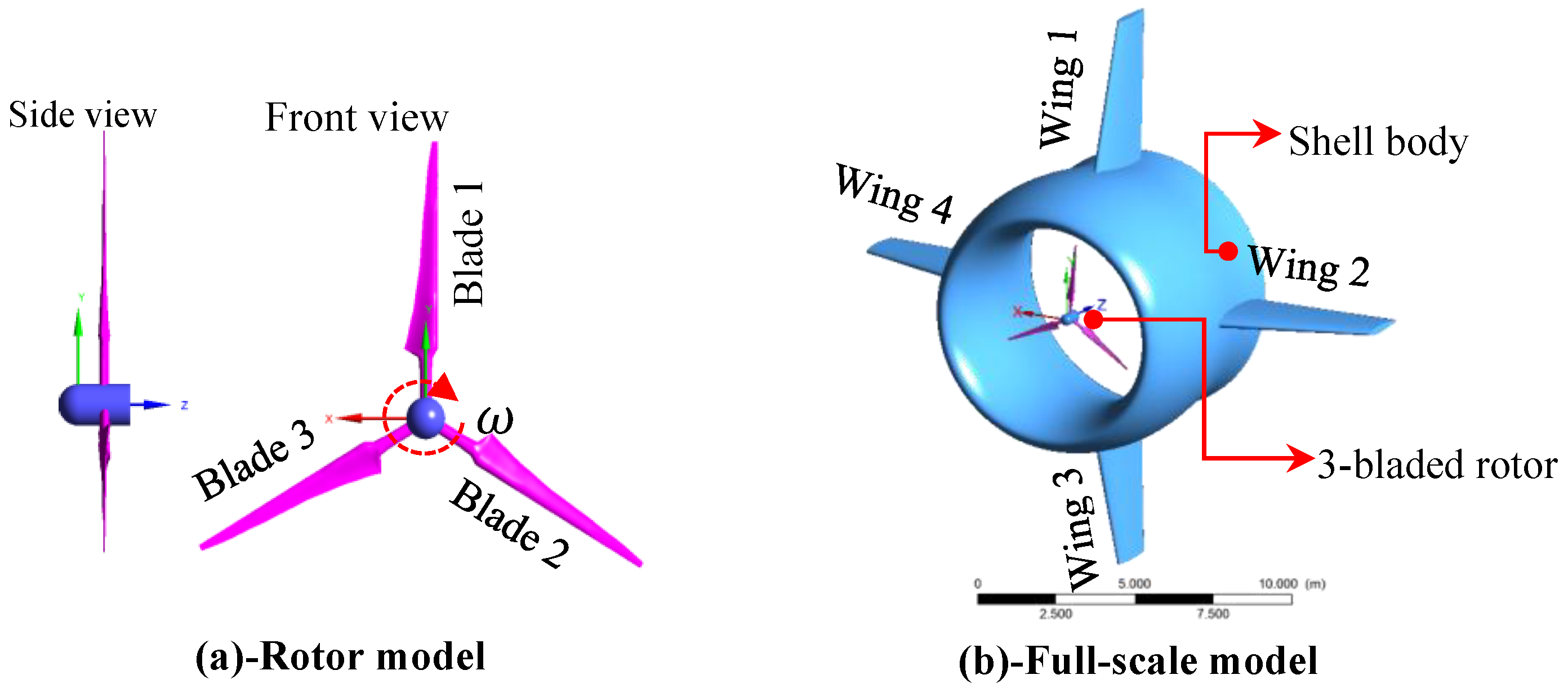
Figure 2.
One-way fluid-structure interaction (FSI) analysis of airborne energy system.
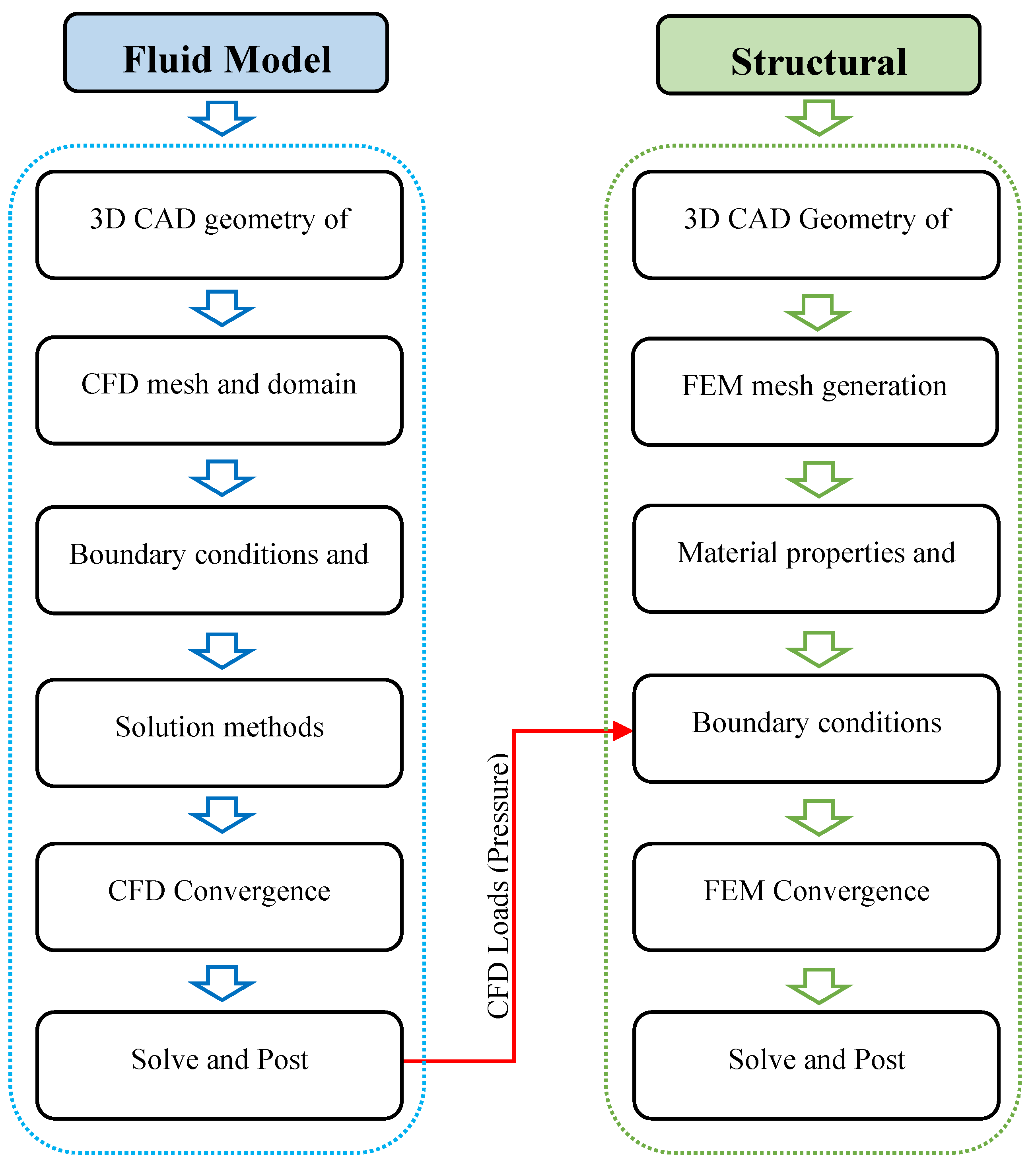
Figure 3.
Detail description of blade (spanwise direction) and shell (axial direction) geometries.
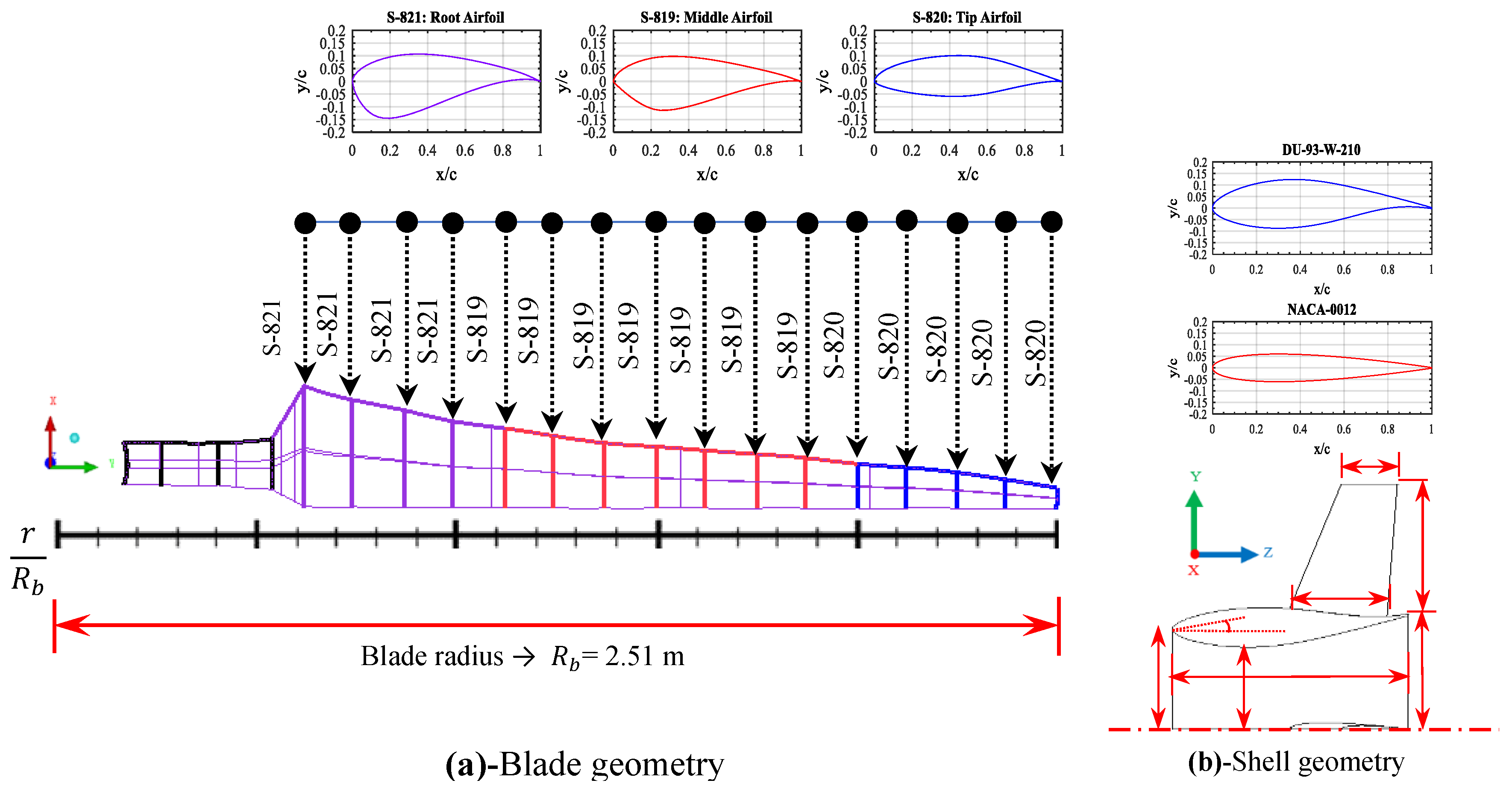
Figure 4.
Various sections of blade and shell surface geometries.
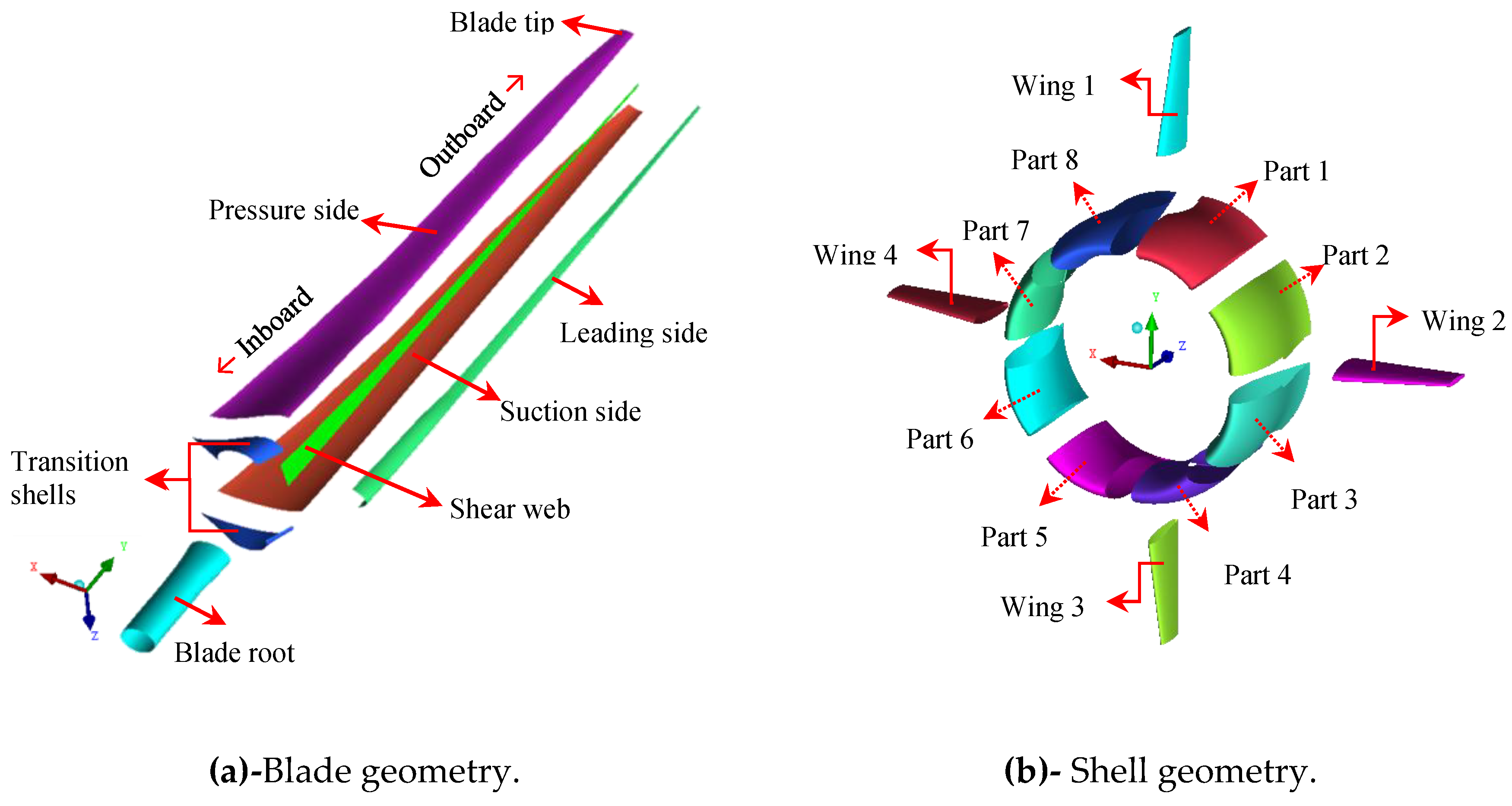
Figure 5.
Description of mesh models of blade and shell in CFD and FEM modelings.
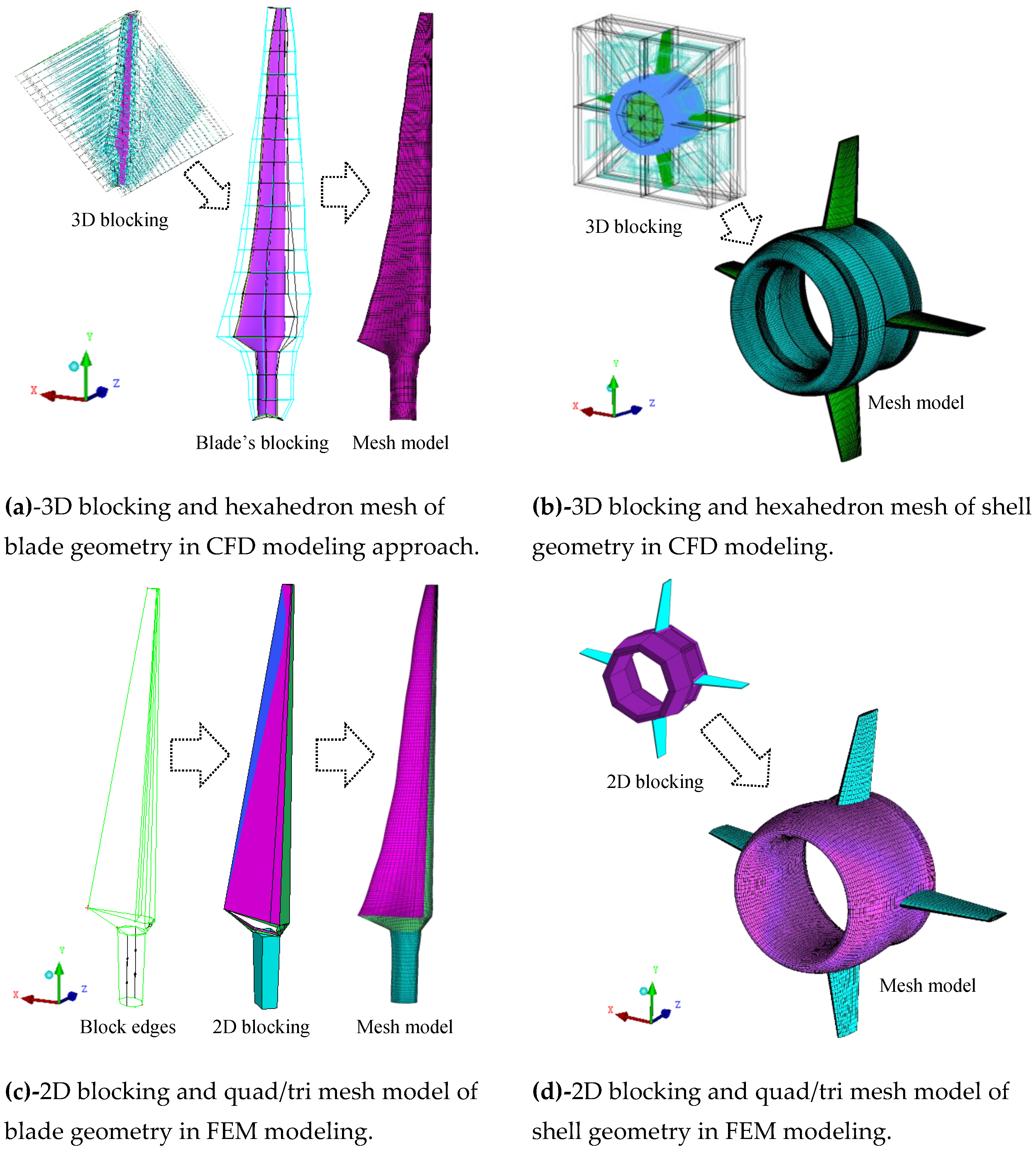
Figure 6.
Computational domain and boundary conditions (BCs) in CFD and FEM modelings.
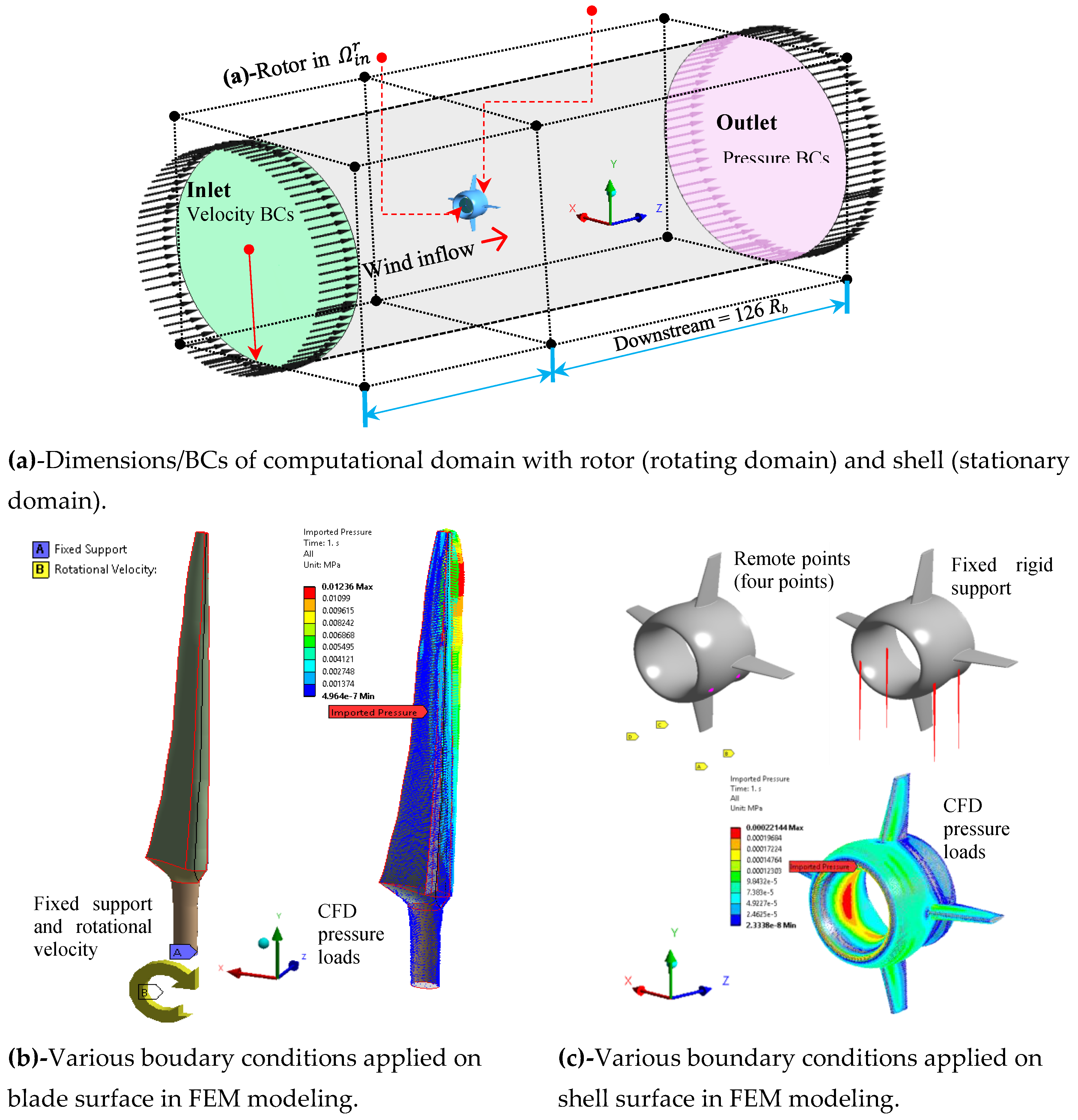
Figure 7.
Configuration of Shell-181 elements and typical material orientation on surface of blade.
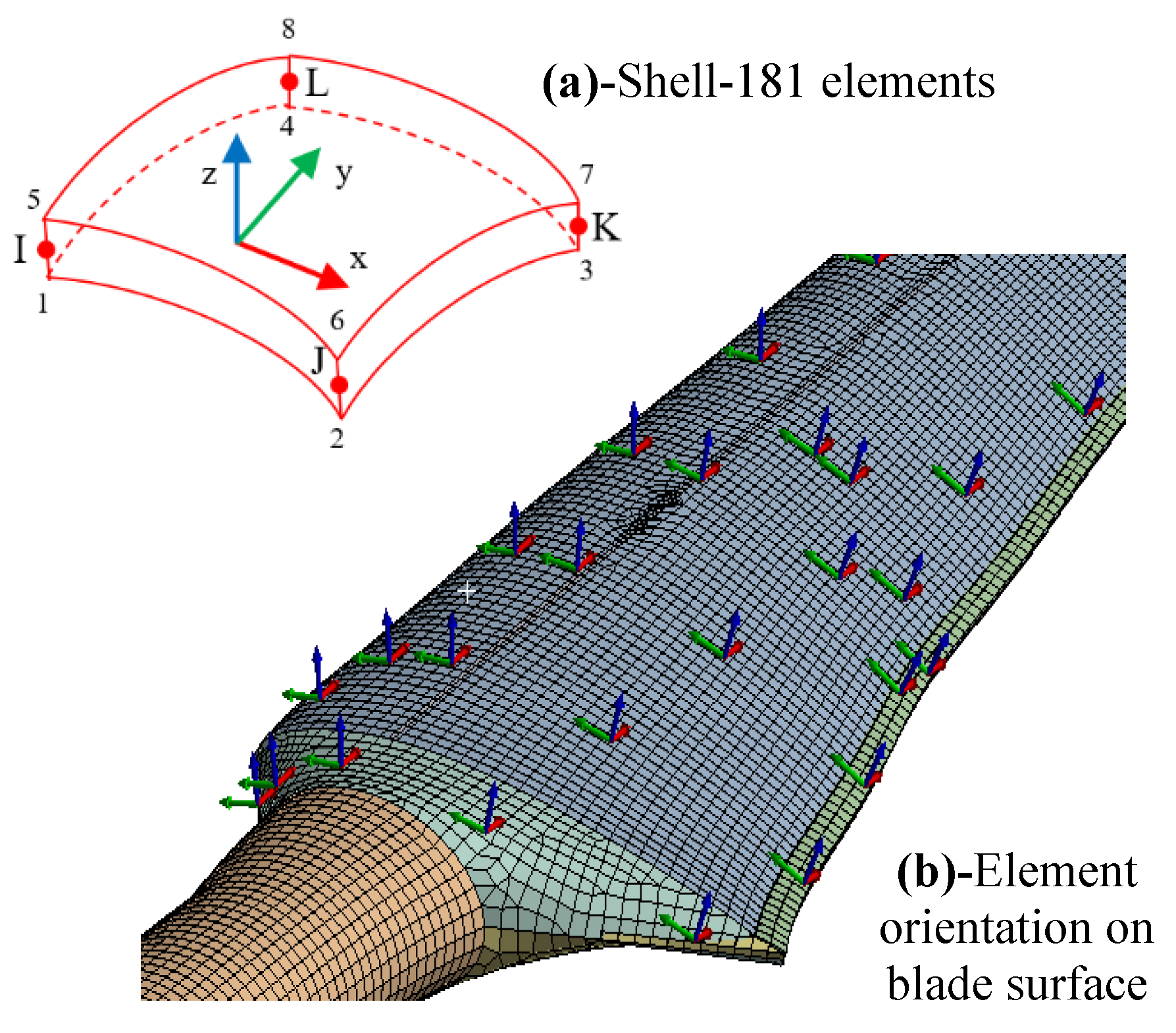
Figure 8.
Distribution of chord length, twist angle, material thickness and mass across blade geometry.
Figure 8.
Distribution of chord length, twist angle, material thickness and mass across blade geometry.
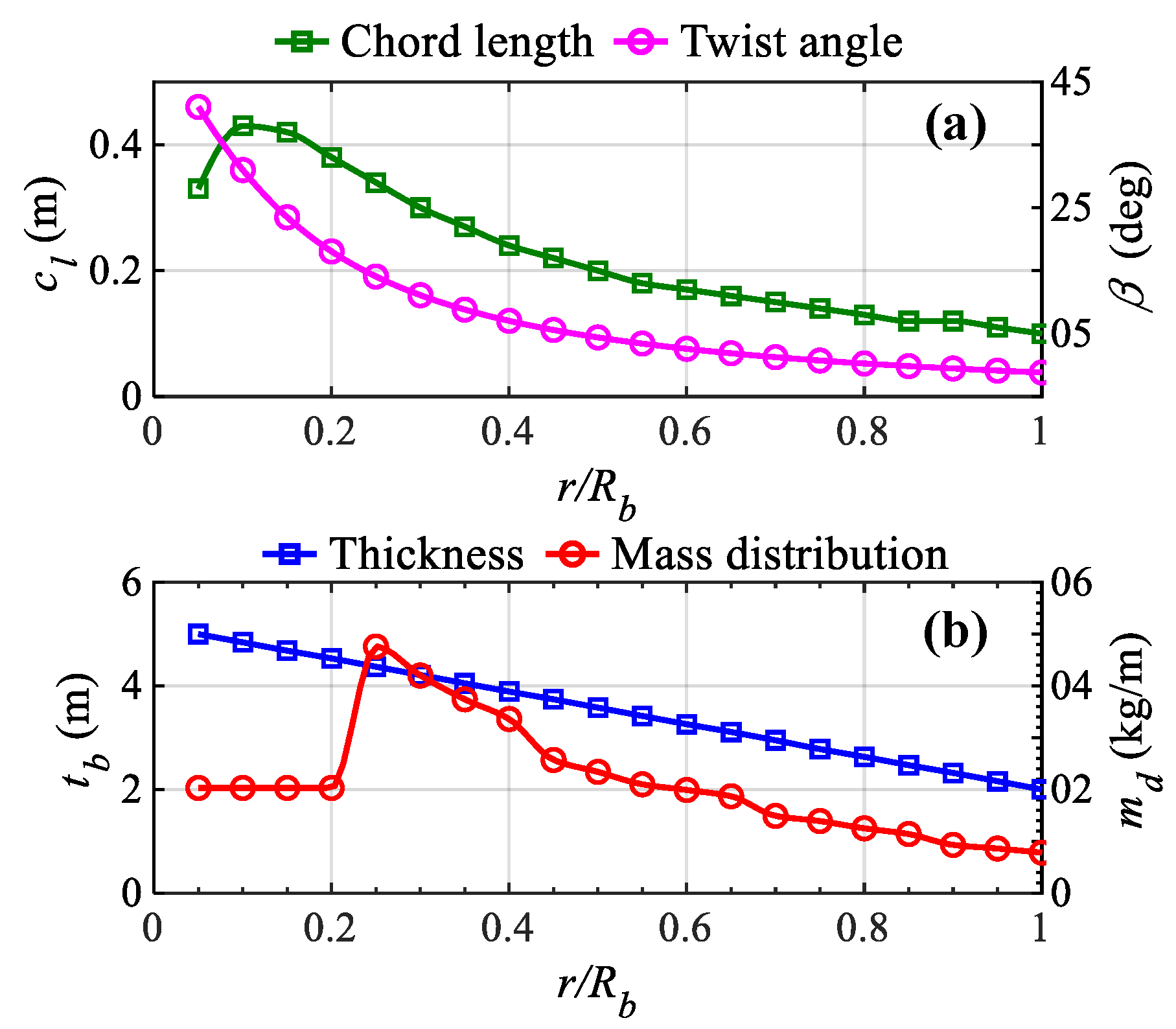
Figure 9.
Validation of fully-resolved CFD model by comparing with airfoil-based ducted models.
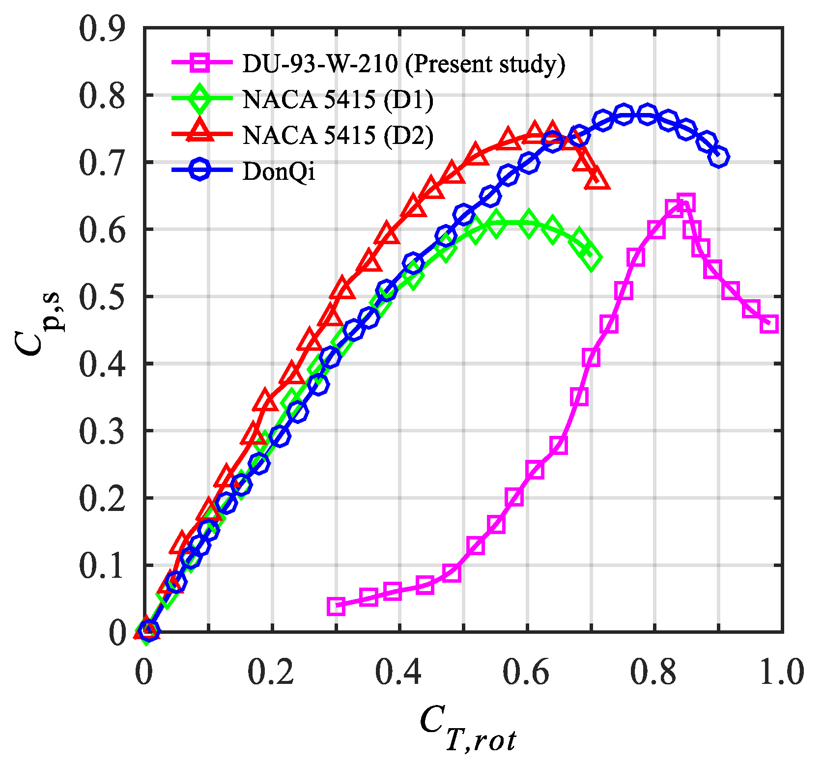
Figure 10.
Validation of FEM blade model by comparing with NuMAD blade models.
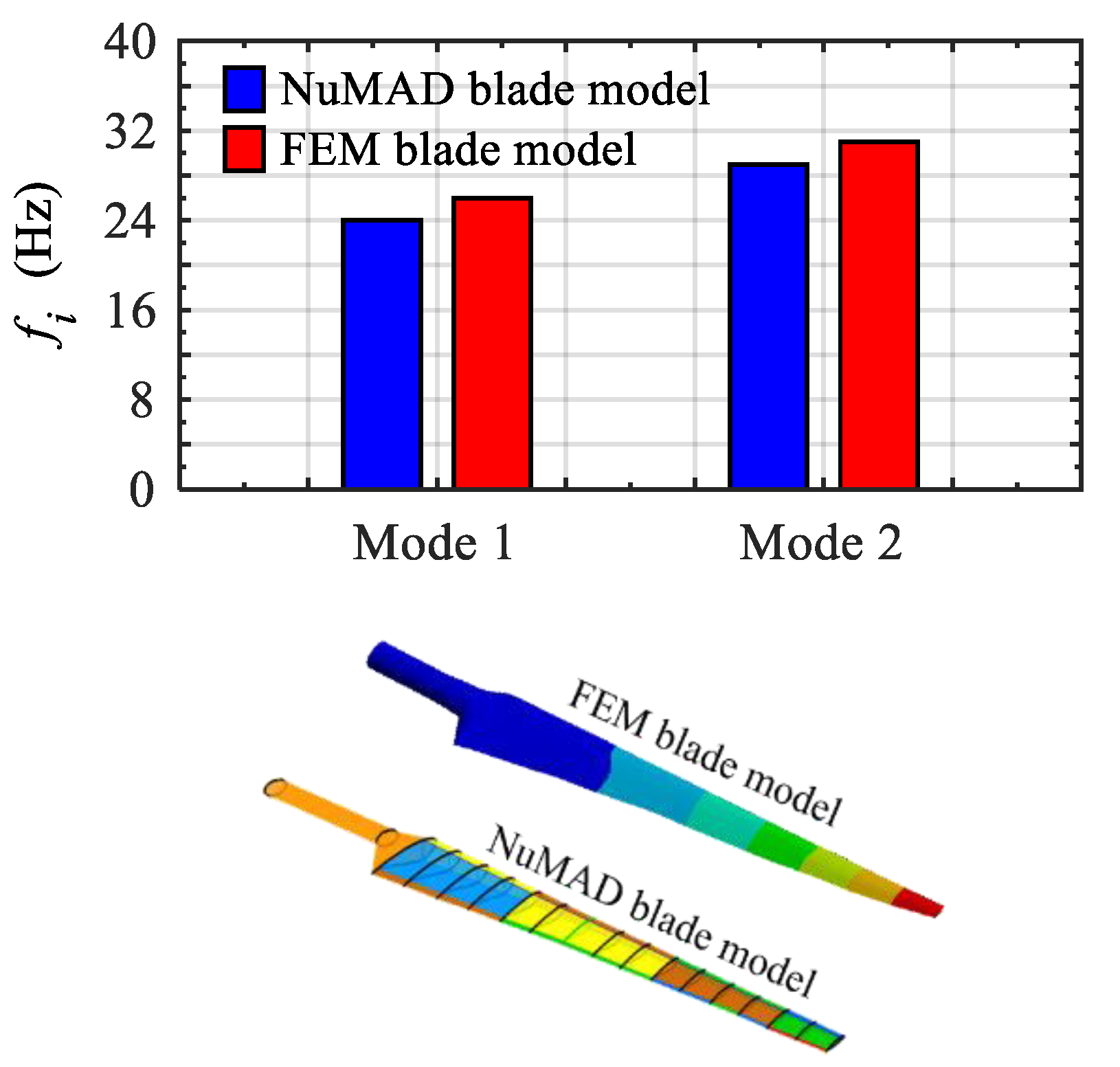
Figure 11.
Flapwise modes of a single blade.
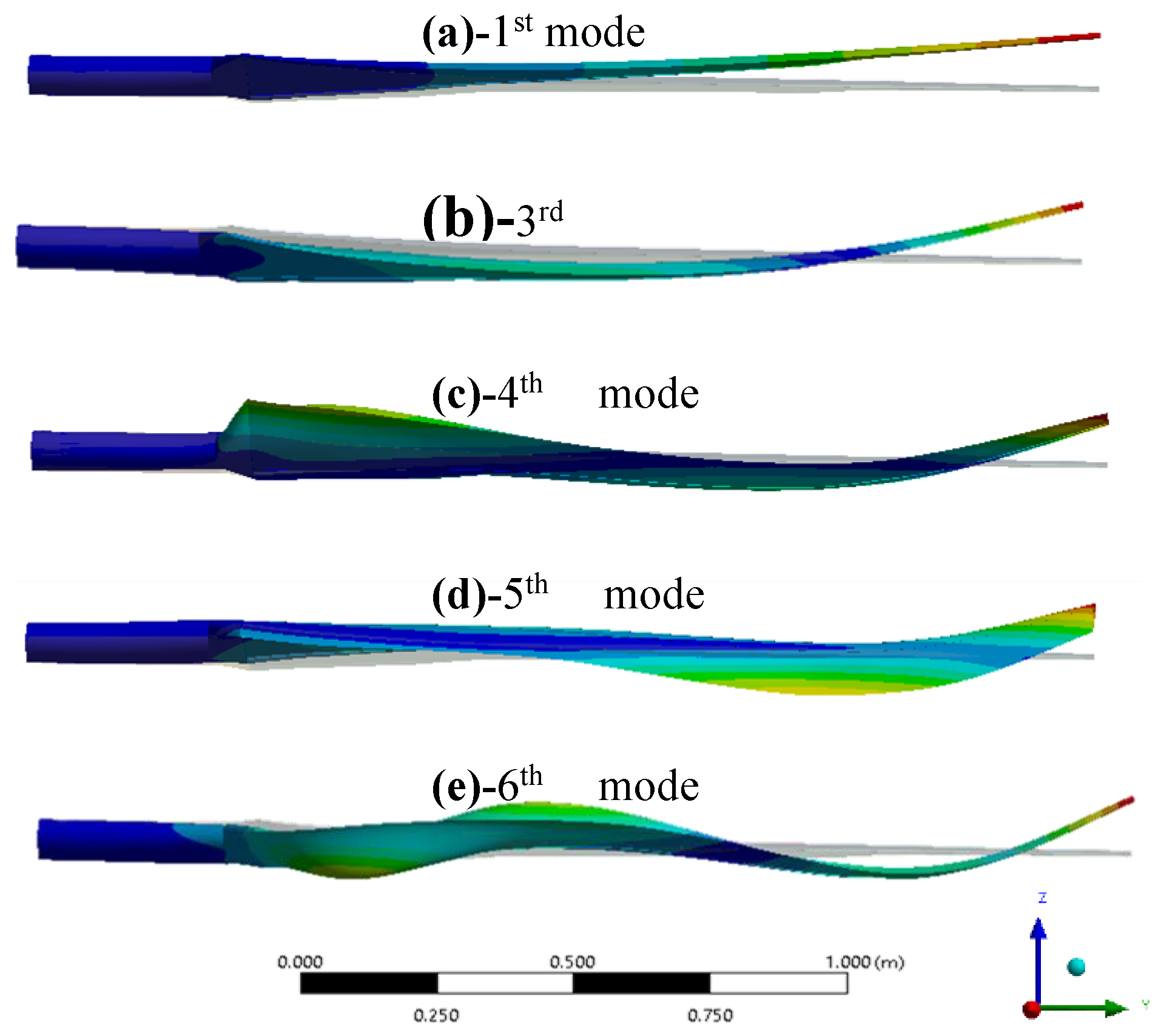
Figure 12.
Edgewise modes of a single blade.
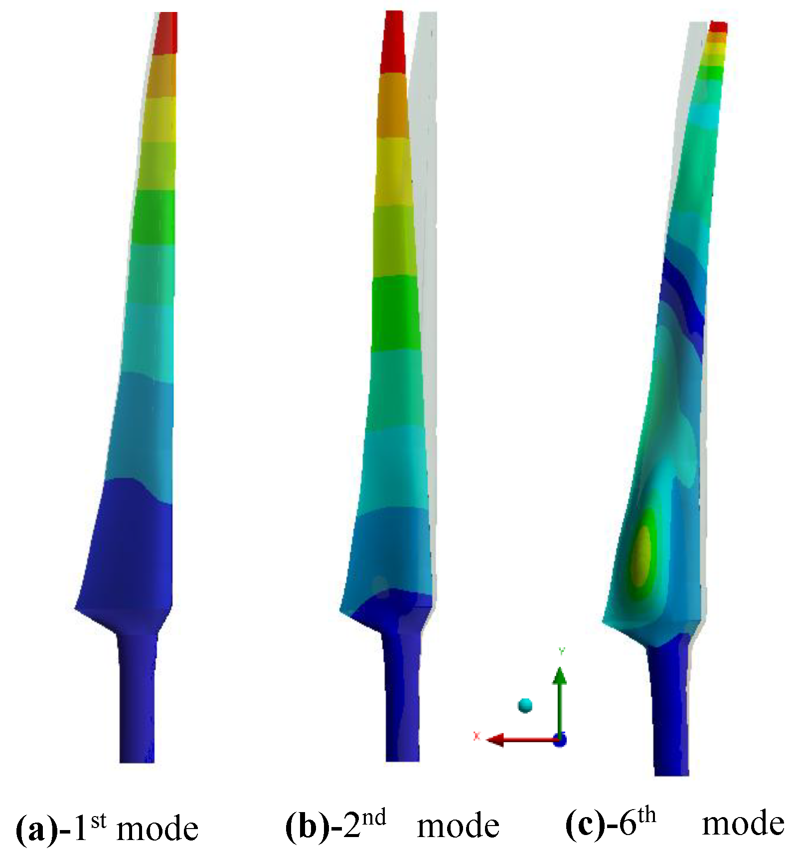
Figure 13.
Performance curves of torque cofficient
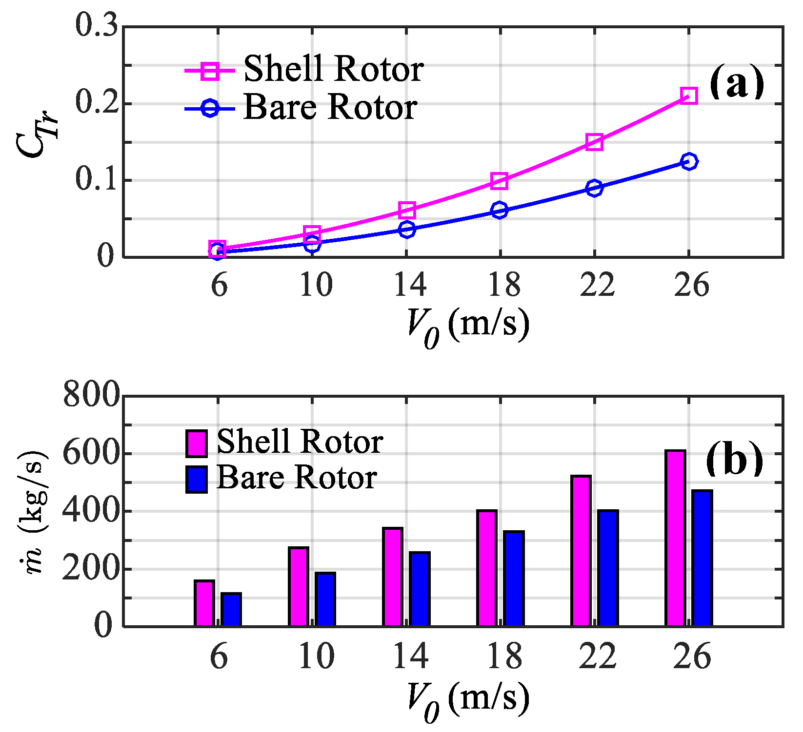
Figure 14.
Normalized velocity and pressure across rotor blade in shell configuration.
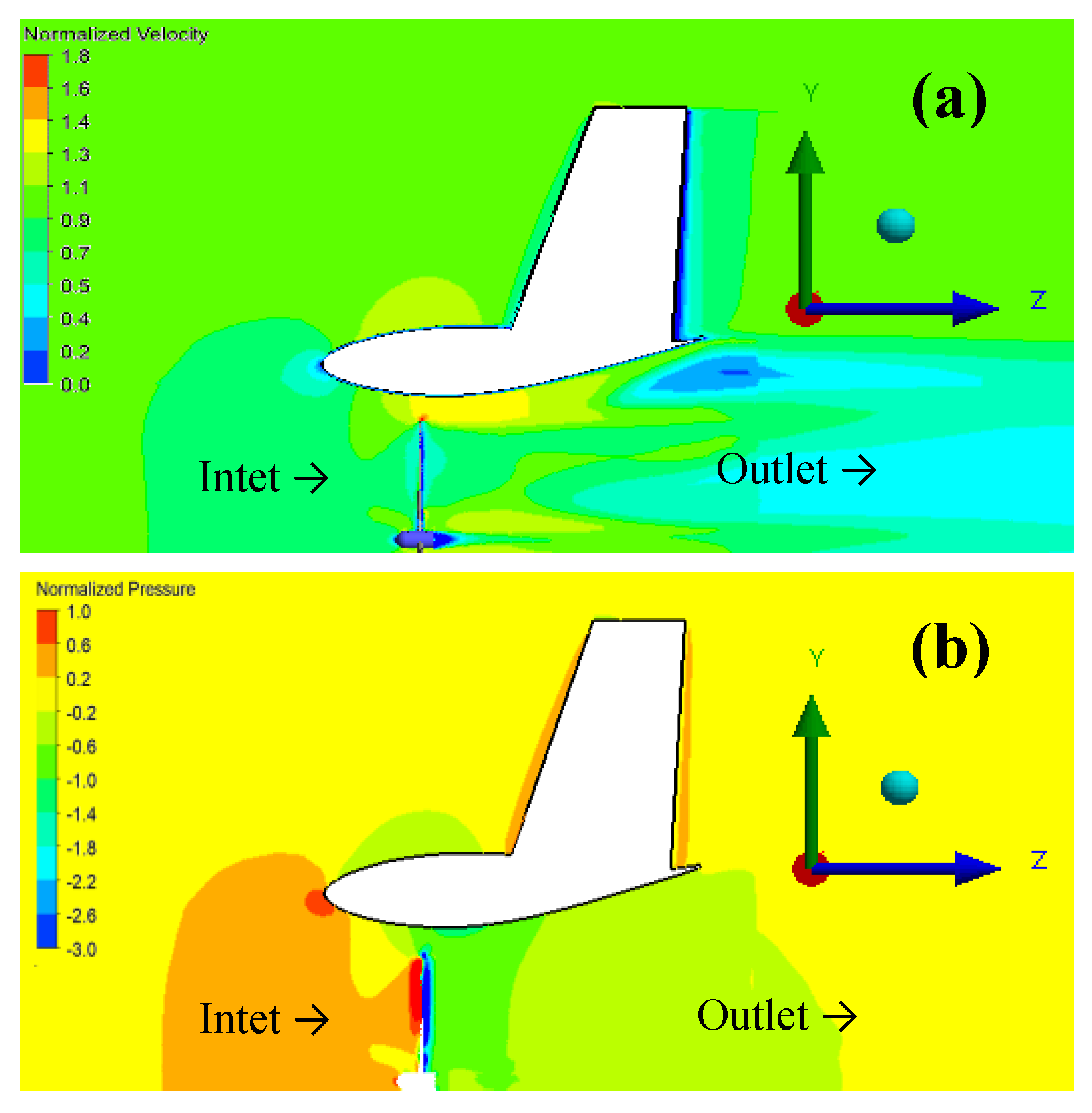
Figure 15.
Spanwise distribution of torque
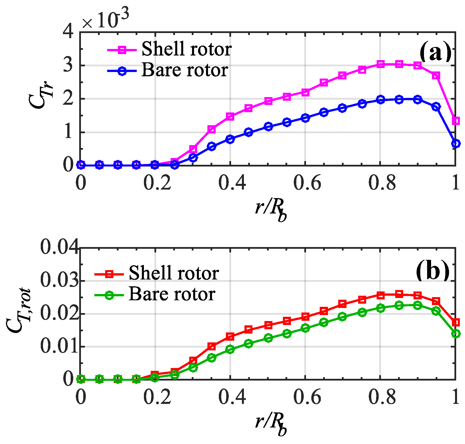
Figure 16.
Azimuth variation of axial, tangential and normal forces on the shell structure.
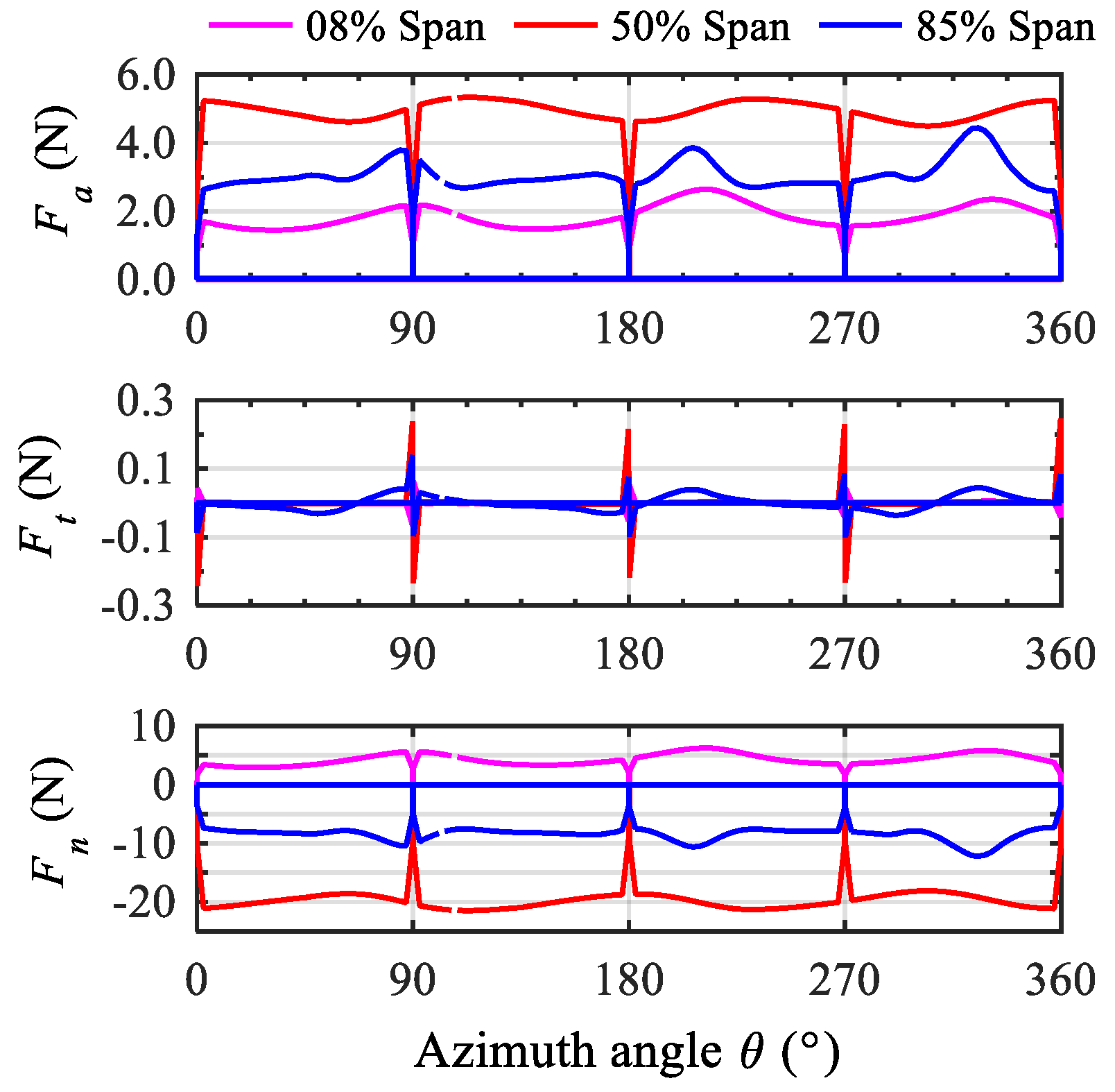
Figure 17.
Total deformation of the blade under bare and shell configuration using various wind velocities.
Figure 17.
Total deformation of the blade under bare and shell configuration using various wind velocities.
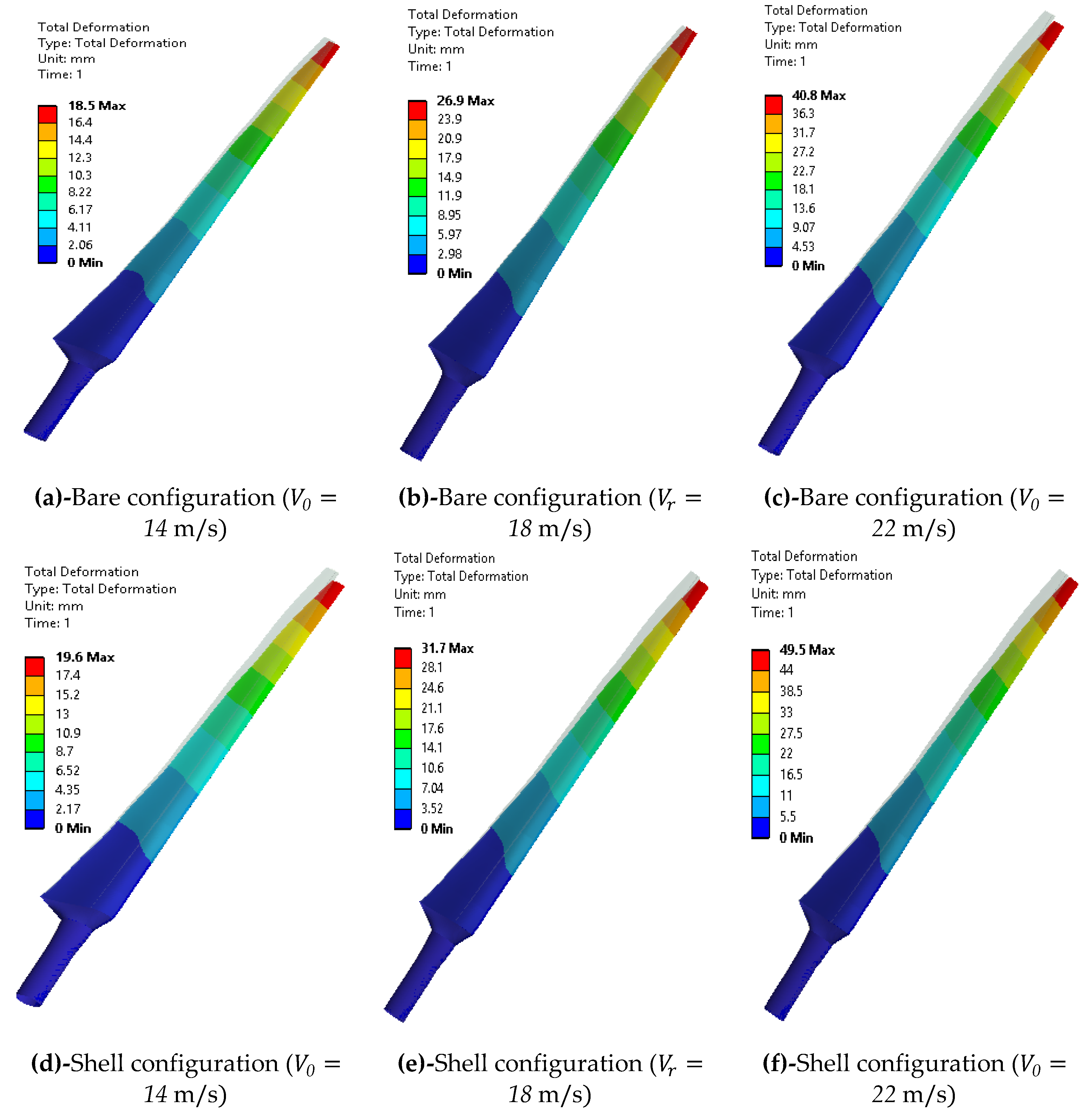
Figure 18.
Directional stresses on the blade surface in bare rotor and shell rotor.
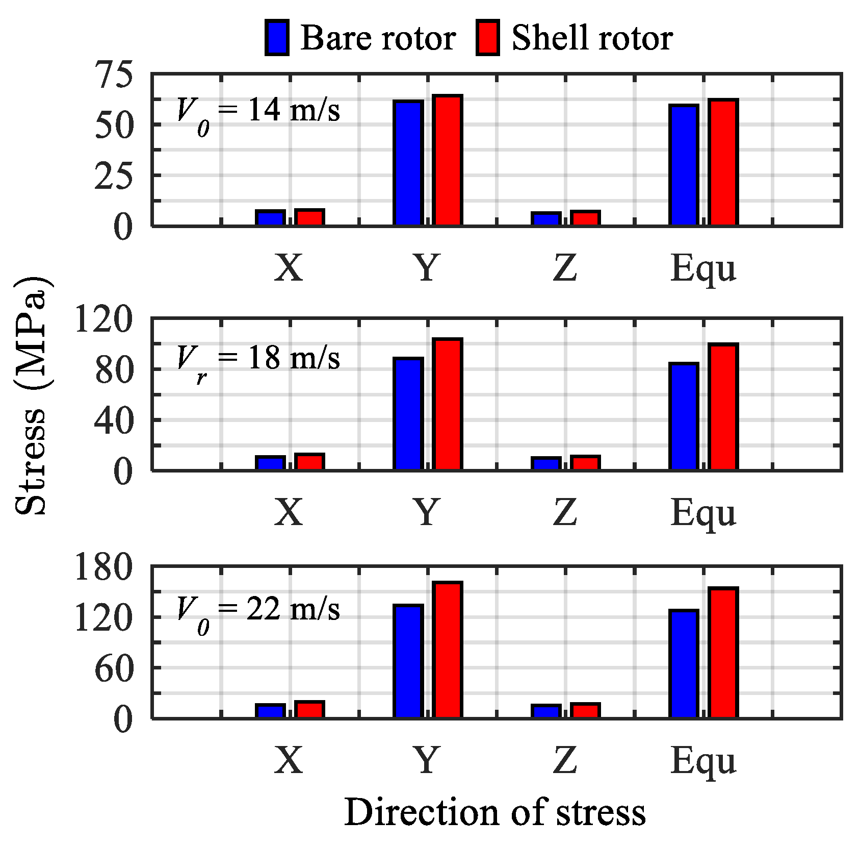
Figure 19.
Mapping of normalized stress and strain along a span of the shear web in bare and shell rotors.
Figure 19.
Mapping of normalized stress and strain along a span of the shear web in bare and shell rotors.
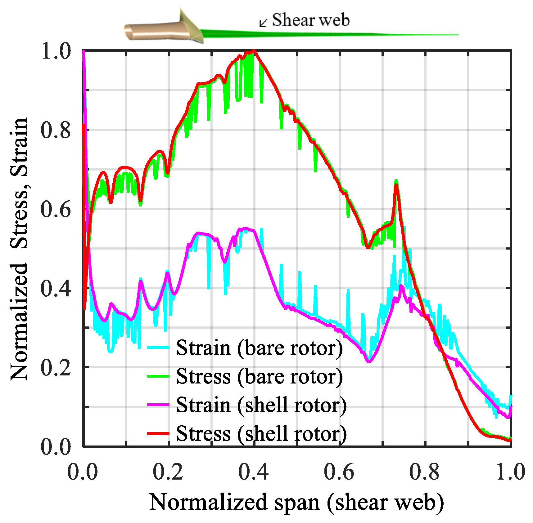
Figure 20.
Campbell diagram of the rotor with various rotational speeds and related natural frequencies.
Figure 20.
Campbell diagram of the rotor with various rotational speeds and related natural frequencies.
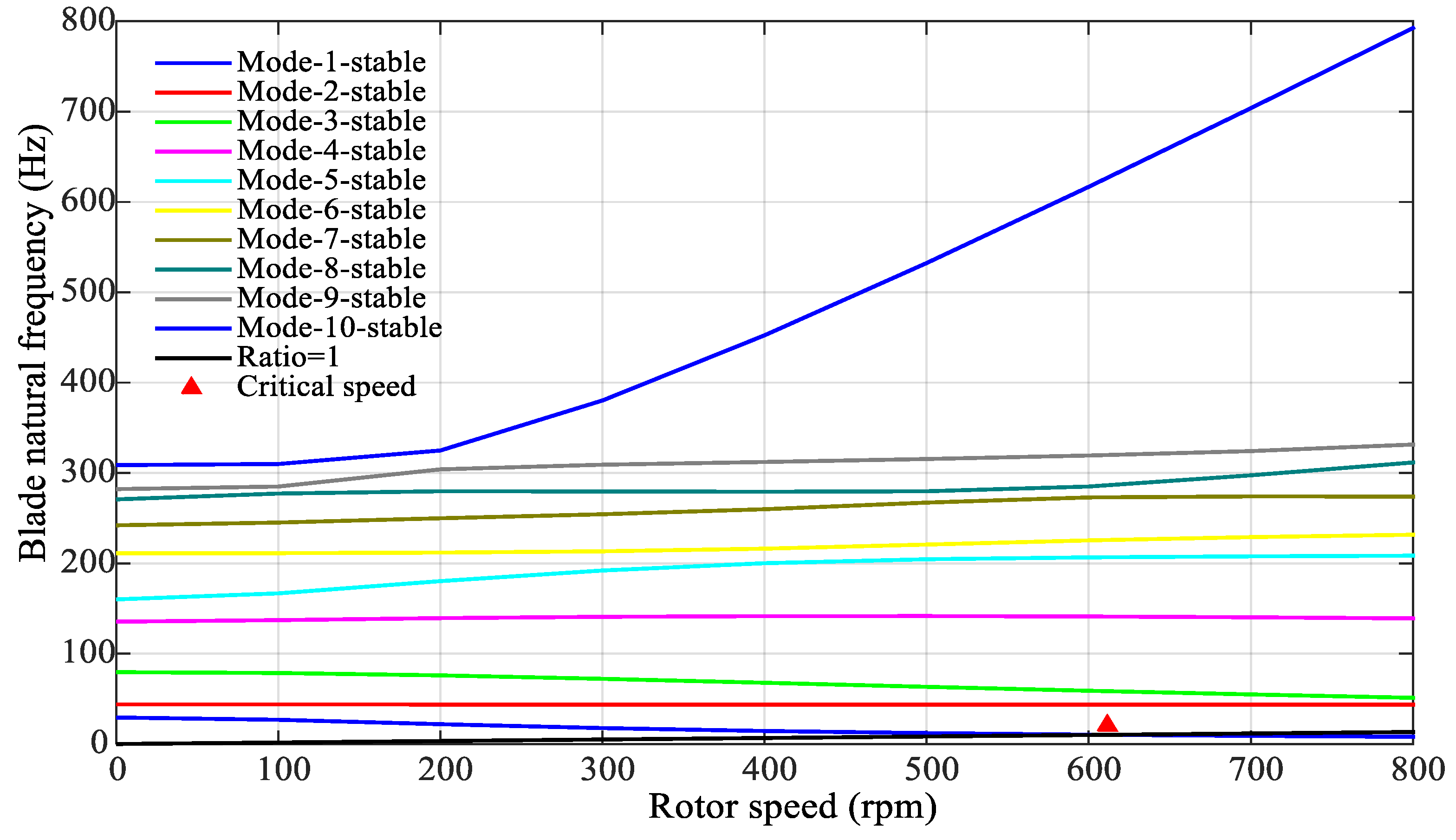
Figure 21.
Total deformation on the true scale of shell structure under various wind loads.
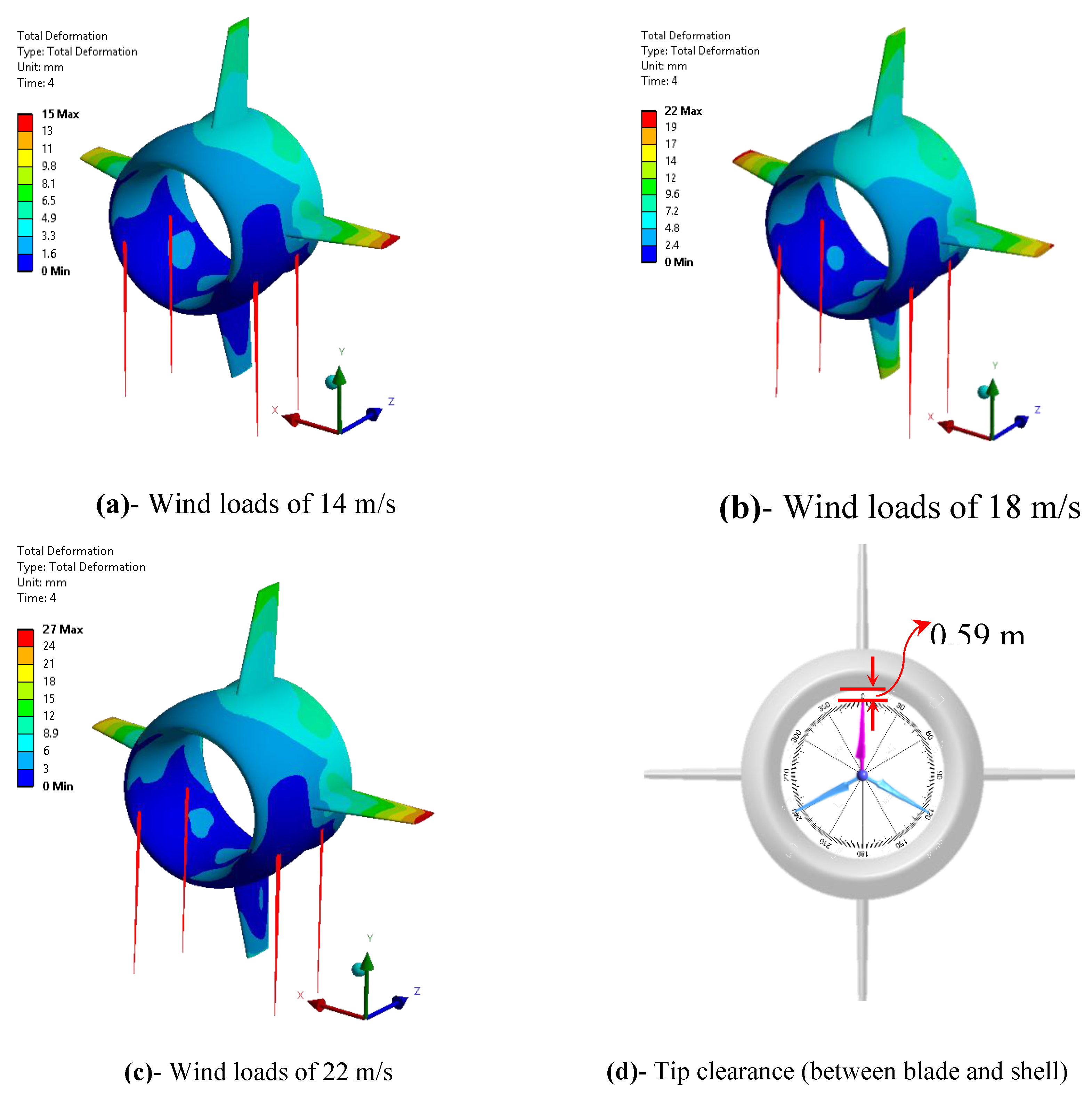

Table 1.
Specifications of rotor and shell in BAT energy system.
| Rotor specification | Shell specifications | ||||||
| Description | Parameter | Value | Units | Description | Parameter | Value | Units |
| Rated power output | 30 | kW | Payload (rotor + shell) | 75 | kg | ||
| Power coefficient | 0.48 | – | Generator + drivetrain | 120 | kg | ||
| Blade radius | 2.51 | m | Helium gas weight | 35 | kg | ||
| Rated TSR | 6.5 | – | Factor of safety | 1.2 | – | ||
| Wind speed (rated) | 18 | m/s | Total downward force | 2.70 | kN | ||
| Air density (400 m) | 1.179 | kg/m3 | Shell volume | 155 | m3 | ||
| Generator efficiency | 92 | % | Gravitational force | 9.81 | m/s2 | ||
Table 2.
Material properties table for blade and shell.
| Material | ρ | Ex | Ey | Ez | Gxy | Gyz | Gxz | νxy | νyz | νxz |
| Units | (Kg/m3) | (GPa) | (GPa) | (GPa) | (GPa) | (GPa) | (GPa) | (-) | (-) | (-) |
| Blade’s material | 1500 | 110 | 7.60 | 7.60 | 5.45 | 2.95 | 2.95 | 0.32 | 0.36 | 0.35 |
| Shell’s material | 1440 | 124 | - | - | - | - | - | 0.36 | - | - |
Table 3.
CFD mesh sensitivity analysis of rotor and shell structure.
| CFD mesh results of rotor blades | |||||
| Total mesh elements → | 12 million | 15 million | 17 million | 20 million | % diff |
| Parameter (units)↓ | mesh 1 | mesh 2 | mesh 3 | mesh 4 | |
| Mechanical torque (Nm) | 533 | 548 | 567 | 572 | 0.88 |
| Single iteration time (s) | 145 | 188 | 224 | 249 | 10.57 |
| CFD mesh results of shell | |||||
| Total mesh elements → | 07 million | 08 million | 09 million | 10 million | % diff |
| Parameter (units)↓ | mesh 1 | mesh 2 | mesh 3 | mesh 4 | |
| Axial force (N) | 668 | 677 | 685 | 691 | 0.87 |
| Single iteration time (s) | 331 | 343 | 350 | 368 | 5.01 |
Table 4.
FEM mesh blade sensitivity analysis of blade.
| Mesh elements → | 22,973 | 36,626 | 74,404 | 1,67,065 | % diff |
| Natural frequency (units) mode ↓ | mesh 1 | mesh 2 | mesh 3 | mesh 4 | |
| Natural frequency (Hz) mode 1 | 30.50 | 30.54 | 29.36 | 29.55 | 0.63 |
| Natural frequency (Hz) mode 2 | 45.81 | 45.84 | 43.93 | 44.18 | 0.58 |
| Natural frequency (Hz) mode 3 | 79.43 | 79.49 | 79.52 | 79.83 | 0.39 |
| Natural frequency (Hz) mode 4 | 134.57 | 134.61 | 135.41 | 135.64 | 0.16 |
| Natural frequency (Hz) mode 5 | 160.17 | 160.24 | 160.05 | 160.37 | 0.19 |
| Natural frequency (Hz) mode 6 | 208.42 | 208.54 | 211.06 | 211.54 | 0.22 |
Disclaimer/Publisher’s Note: The statements, opinions and data contained in all publications are solely those of the individual author(s) and contributor(s) and not of MDPI and/or the editor(s). MDPI and/or the editor(s) disclaim responsibility for any injury to people or property resulting from any ideas, methods, instructions or products referred to in the content. |
© 2025 by the authors. Licensee MDPI, Basel, Switzerland. This article is an open access article distributed under the terms and conditions of the Creative Commons Attribution (CC BY) license (http://creativecommons.org/licenses/by/4.0/).
Copyright: This open access article is published under a Creative Commons CC BY 4.0 license, which permit the free download, distribution, and reuse, provided that the author and preprint are cited in any reuse.


