
Submitted:
03 October 2025
Posted:
07 October 2025
You are already at the latest version
Abstract
In recent years, the rapid rise in the popularity of cryptocurrencies has drawn increasing attention from investors, entrepreneurs, and the public. However, this rapid growth comes with risk: Many coins fail early and become what are known as ``dead coins", defined by a lack of recorded activity for more than a year. A substantial number of cryptocurrencies fail to reach the one-year mark, leading to significant financial losses for investors. This study compares deep neural network architectures Long Short-Term Memory (LSTM), Bidirectional LSTM (BiLSTM), and Gated Recurrent Unit (GRU) to estimate the likelihood of a coin's failure within 10 days. Among the three models, LSTM exhibited the most fluctuating and comparatively lower performance. Using the previous 180 days of data as input, GRU achieved the highest point accuracy of 0.7134, whereas BiLSTM exhibited the best performance when evaluated across input sequence lengths varying from 10 to 180 days, reaching an average accuracy of 0.676. These findings show how recurrent architectures can be used to anticipate short-term failures in cryptocurrency markets.
Keywords:
LSTM
; BiLSTM
; GRU
; cryptocurrency
; time series classification
; dead coins
1. Introduction
Cryptocurrencies are financial assets that exist in digital form and use cryptography for secure transactions within a decentralized system. In recent years, cryptocurrencies have gained popularity due to advantages such as enabling peer-to-peer transactions without intermediary financial institutions and providing secure and private financial transfers [24]. Bitcoin was the first cryptocurrency emerging with this notion, which was presented as a purely peer-to-peer version of electronic cash [25]. Since Bitcoin, millions of other cryptocurrencies have been created. As of July 2025, cryptocurrency tracking website CoinMarketCap stated the total number of cryptocurrencies tracked as 18.67 million [5]. One of the main reasons behind the popularity of cryptocurrencies is their potential to generate substantial long-term profit for investors. For example, Bitcoin’s price has increased roughly tenfold over the last five years, despite experiencing periods of sharp volatility during that time [8]. As noted by some cryptocurrency supporters, investors also appreciate that cryptocurrencies eliminate the need for central banks to control the money supply, since such banks are often linked to inflation and a decline in money’s value. [29].
Although cryptocurrencies can yield high returns, they are also highly susceptible to significant losses in value due to the fluctuating nature of the cryptocurrency market. Fluctuations in the value of a cryptocurrency may result from macroeconomic factors that influence the overall financial landscape, while they can also be affected by characteristic parameters of a coin, such as market activity, trading volume, closing price, opening price, and similar indicators. On the macroeconomic side, high interest rates might motivate investors to move their money from low-utility or speculative coins to safer assets, such as savings accounts. Similarly, during times of uncertainty, such as wars or economic crises, people tend to avoid risky financial moves, which can affect the cryptocurrency market. According to a case study, the start of the COVID-19 pandemic caused a crypto-rush, followed by an inverse trend as many investors left the market [20]. Such events can also result in the disappearance of certain cryptocurrencies from the market. Many other factors, such as the level of trust given to investors by the founder of a cryptocurrency, negative social media sentiments, or scandals, can lead to a rapid decline in a coin’s trading volume. For example, a leading cryptocurrency exchange, FTX, crashed in November 2022 after it was revealed that its affiliate, Alameda Research, relied heavily on speculative tokens [28]. This led to the withdrawals of many customers and the bankruptcy of both companies, causing significant disruption in the cryptocurrency market. Aside from scams, cryptocurrencies that are created as jokes or memes often lose their validity due to lack of practicality, while legitimate coins can become dead coins due to insufficient funding, developer departure, or declining market interest [22].
A cryptocurrency that has lost almost all its value or is no longer usable is known as a “dead coin" [22]. According to industry standards, cryptocurrencies are usually categorized as defunct or “dead" if their trading volume over three months is less than $1,000 [22]. Within the scope of this study, a dead coin is defined as a cryptocurrency with no activity within the past year. While there are many external factors affecting the value fluctuations and death of a cryptocurrency, these factors are hard to track and use for future predictions. On the other hand, quantitative parameters of a coin, categorized as time series data, can provide insights into whether the coin will continue to be traded or lose its value over time. These predictions can be useful for investors to manage their cryptocurrency portfolios and minimize potential losses.
In the context of time series, the goal of forecasting is to predict exact values, whereas classification assigns data to distinct categories based on its past behavior. Time Series Classification (TSC) is the task of training a classifier with sequential time series data to learn a mapping from input sequences to a probability distribution over possible class labels [9]. In many real-world scenarios, especially financial applications, classification of data can be more useful for decision-making than forecasting. This change in approach has led to the development of many TSC methods, particularly for use in finance.
This study places special emphasis on classifying time series data by predicting whether a cryptocurrency will become dead within the upcoming 10-day period. By analyzing the risk of cryptocurrencies’ dying, investors can reduce potential losses and enhance their portfolio management strategies. The classifications were based solely on the coins’ characteristics, specifically daily closing prices and trading volumes. We retrieved the time series data used in this study from Nomics1.
Historically, TSC problems have been solved with various methodologies such as k-Nearest Neighbors (k-NN), and Dynamic Time Warping (DTW) [1,35]. In more recent years, machine learning and deep learning methodologies have surfaced and they have been used for many time series forecasting and classification problems. Recurrent Neural Networks (RNNs) are particularly useful for capturing temporal patterns between data; hence, they are commonly used for sequential prediction problems [33]. In a study comparing various machine learning and deep learning models for forecasting Bitcoin price trends, RNNs were found to outperform other architectures, highlighting their effectiveness for cryptocurrency-related prediction tasks [14]. Among them, the Long Short-Term Memory (LSTM) and Gated Recurrent Unit (GRU) models demonstrated particularly strong performance, further supporting their suitability for modeling financial time series data. Therefore, LSTM, GRU, and Bidirectional LSTM (BiLSTM) architectures, which are specific forms of RNN, are selected in this study to assess their performance in predicting the risk of cryptocurrencies becoming dead coins.
The main objectives of this study can be summarized as follows:
- Creating variations of deep learning models using LSTM, GRU, and BiLSTM architectures by systematically altering the number of layers and units per layer to analyze their impact on predictive performance.
- Training these models with time series data of trading volume and closing price values of cryptocurrencies to predict the risk of a coin becoming dead within the following 10 days, and selecting the best-performing model for each architecture.
- Comparing the model performances across historical input windows of 10 to 180 past days to evaluate how the length of past data influences the performance of predicting a coin’s death risk within the following 10 days.
The remainder of this paper is organized as follows: Section 2 gives insights about the related work. Section 3 describes the dataset used in the study and its related preprocessing steps. Section 4 explains the deep learning architectures used in the experiments. Section 5 outlines the details of the experiment procedure and analyzes the results. Finally, the study is concluded with Section 6.
2. Related Work
Data instances recorded sequentially over time are referred to as time series data, which consist of ordered data points that carry meaningful information [9]. Time series data are useful for handling forecasting and classification tasks, enabling models to capture temporal patterns and trends over time. Therefore, it is applied in a wide range of fields, such as anomaly detection [23], weather prediction [36], and public health monitoring, including but not limited to predicting the transmission of COVID-19 [4]. Financial forecasting is also a key area that benefits from historical financial time series data to predict trends in the market to provide strategical insights to investors and speculators [32].
In early approaches to time series forecasting, statistical models, such as Autoregressive Integrated Moving Average (ARIMA), were used. A linear dynamic model can often provide a reasonable approximation for serial dependence in time series data, and ARIMA captures linear dependencies through autoregressive (AR) and moving average (MA) components [34]. Seasonal ARIMA (SARIMA) extends ARIMA to address seasonal patterns commonly seen in economic and business time series [34]. Furthermore, ArunKumar et al. [3] conducted a study in which the ARIMA and SARIMA models were used to predict the epidemiological trends of the COVID-19 pandemic in the top 16 countries that account for 70%–80% of global cumulative cases. Although conventional statistical models such as ARIMA and SARIMA have been extensively applied for time series forecasting, they are constrained by their assumption of linearity [3].
Machine learning methods have emerged as effective alternatives to statistical models in recent years, primarily due to their ability to capture complex, nonlinear relationships within time series data. One of the most commonly applied classification techniques is k-Nearest Neighbors (k-NN), known for its simplicity and effectiveness in time series classification tasks [1,6]. Another widely-adopted methodology is Dynamic Time Warping (DTW), which is a method to measure the similarity between two time series [35]. DTW has proven valuable in various domains, particularly in financial time series classification. For example, the study by [16] demonstrated that DTW can be used to extract short-term patterns from stock time series for analysis of stock trends. Additionally, [15] introduced the DTW algorithm as a key financial risk detection tool, emphasizing its effectiveness in identifying similarities within time series data, including that obtained from sensor networks.
Building on these classical approaches, neural networks have gained popularity for time series forecasting and classification tasks. Recurrent Neural Networks (RNNs) are the most widely used machine learning models for sequential prediction problems [33]. Within the family of RNNs, Long Short-Term Memory (LSTM) and Gated Recurrent Unit (GRU) architectures are widely used for modeling long-term dependencies in time series data, as they effectively address challenges such as vanishing gradients [17]. These architectures have become popular for time series forecasting applications due to their ability to capture complex temporal patterns. For instance, [10] developed LSTM-based models for stock trading, achieving robust portfolio performance in the German financial market. Similarly, [31] trained LSTM and GRU networks using the technical indicators (TI) and open, high, low, and close (OHLC) features of various stocks to predict the opening prices of the stocks for the following day. In this study, GRU achieved higher accuracy in most cases, reducing Mean Absolute Percentage Error (MAPE) to 0.62% for Google stock, compared to LSTM’s 1.05%. Likewise, [21] constructed eight models with different preprocessing and regularization steps for forecasting the stock prices of the companies AMZN, GOOGL, BLL, and QCOM. Although the models showed competing performance, it was significant that the four models combined with GRU outperformed the other four models combined with LSTM on the stock prices of AMZN, GOOGL, BLL, and QCOM with accuracies of 96.07%, 94.33%, 96.60%, and 95.38%, respectively.
Time series analysis can be applied to study cryptocurrency performance, and many studies already focus on forecasting their future values. Some of these studies propose hybrid deep learning approaches for cryptocurrency price prediction. For example, [27] proposed a hybrid model combining LSTM and GRU to forecast Litecoin and Monero prices over the next 1, 3, and 7 days. Although the proposed model did not present an effective result for the next 7 days, it outperformed traditional LSTM by reducing the Mean Squared Error (MSE) from 194.4952 to 5.2838 for Litecoin and 230.9365 to 10.7031 for Monero for 1-day forecasts, demonstrating strong performance for short-term price prediction. In another research, [7] integrated encoder–decoder principle with LSTM and GRU along with multiple activation functions and hyperparameter tuning for trend predictions in the stock and cryptocurrency market. For various individual stocks, stock index S&P, and Bitcoin as a cryptocurrency, autoencoder-GRU (AE-GRU) architecture significantly outperformed autoencoder-LSTM (AE-LSTM) architecture with higher prediction accuracy. In particular, AE-GRU obtained 0.5% MAPE for Bitcoin trend prediction, which is half of the value found in AE-LSTM. In another study, four methods, that are convolutional neural network (CNN), hybrid CNN-LSTM network (CLSTM), multilayer perceptron (MLP), and radial basis function neural network (RBFNN), were compared to predict the trends of six cryptocurrencies, including Bitcoin, Dash, Ether, Litecoin, Monero, and Ripple, within the next minute using 18 technical indicators. For all cryptocurrencies, CLSTM outperformed other architectures with an accuracy of 79.94% on Monero and 74.12% on Dash cryptocurrencies [2].
In another study, [11] examined the performance of LSTM in predicting the prices of Electro-Optical System (EOS), Bitcoin, Ethereum, and Dogecoin cryptocurrencies only using their historical closing prices. The results were compared to ARIMA approach using the RMSE (Root Mean Squared Error) metric. LSTM outperformed ARIMA for all cryptocurrencies, especially showing a 72-73% of RMSE reduction for EOS and Dogecoin, which have greater fluctuations in their closing prices compared to Bitcoin and Ethereum, demonstrating that LSTM performs significantly well for highly volatile cryptocurrencies. In a comparative study, [30] implemented LSTM, GRU, and BiLSTM trained on the daily closing prices of Bitcoin, Ethereum, and Litecoin cryptocurrencies in the last five years to forecast their prices. RMSE and the MAPE performance metrics were used to analyze the performance of the models, and BiLSTM surpassed other models with a MAPE value of 0.036 for Bitcoin, 0.124 for Ethereum, and 0.041 for Litecoin. Another study by [12] a probabilistic approach referred to as Probabilistic Gated Recurrent Unit (P-GRU) was proposed, incorporating stochasticity into the traditional GRU by enabling the model weights to have their distinct probability distributions in order to tackle the challenge coming from the volatile nature of cryptocurrencies, focusing on the prediction of Bitcoin prices. This novel method outperformed the other simple, time-distributed, and bidirectional variants of GRU and LSTM networks. The study was also expanded to predict the prices of six other cryptocurrencies by using transfer learning with the P-GRU model, contributing to the overall inquiry for cryptocurrency price prediction.
In line with our study, [26] proposed a method for assessing the death risk of cryptocurrencies over 30, 60, 90, 120, and 150 days, based on their past 30-day data of closing prices and daily trading volumes. In this study, simple RNN architecture was used for capturing temporal patterns in the data. The study showed that the probability of identifying dead cryptocurrencies increases with longer prediction windows, starting from roughly 37% for the prediction of death in the next 30 days, and reaching nearly 84% for the 150-day horizon. Building on this research, our study applies special forms of RNN to predict the death risk of cryptocurrencies in the following 10 days using varying number of input days. By providing short-term predictions, this approach may help protect investors from the risk of holding cryptocurrencies that are likely to fail rapidly.
3. Materials and Methods
3.1. Data Description and Preprocessing
The dataset2 is composed of time series data about the cryptocurrencies that died by March 1, 2023. We found 7312 such cryptocurrencies. According to our definition, the last transaction on these dead cryptocurrencies is before March 1, 2022. The dataset includes daily trade volume and closing price values for these cryptocurrencies, collected from various online markets. Data are missing for weekends and holidays.
To complete the time series, missing volume values are set to zero, and missing closing prices are filled in with the closing price of the previous day. In order to be used in the experiments, time series data for at least days are needed, where is the number of past days and is the number of future days. Only cryptocurrencies that have lived for at least 180 days, providing sufficient historical data to generate both positive and negative instances for the largest input window (), are included in the experiments; currencies with shorter lifespans are removed. In all experiments, , since we are interested in predicting if a cryptocurrency will die in the next 10 days. The values we experimented with are 10, 20, 30, 60, 90, 120, 150, and 180. Since both the volume and closing price values have large differences among the cryptocurrencies, we applied z-score normalization to each volume and closing price data for each remaining cryptocurrency.
The problem is to estimate how accurately we can predict if a cryptocurrency will die in the next days, given its time series data from the past days. In preparing the dataset, we opt to have a balanced number of positively and negatively labeled time series data. A positive instance represents the time series data of a cryptocurrency that will live less than days; similarly a negative instance represents the data of a cryptocurrency that will live days or more. Given the time series data for a cryptocurrency, many positive (P-labeled) and the same number of negative (N-labeled) instances are created, as shown in Figure 1. Each instance consists of the time series data of length days. Positive instances are formed from the last days, while negative instances are randomly selected from the previous days.
The number of cryptocurrencies with sufficient data and the number of instances created for each experiment are shown in Table 1.
3.2. Methodology
3.2.1. Long Short-Term Memory (LSTM)
LSTM is a type of RNN, addressing the vanishing gradient problem of conventional RNNs. The architecture of the LSTM cell is displayed in Figure 2. The forget gate selectively removes data that are no longer relevant in the cell state by applying a sigmoid function to the current input and the previous hidden state . Outputs near 0 lead to forgetting, while values near 1 retain information. The input gate adds new information to the cell state by first applying a sigmoid function to and , determining which values to update. It uses a sigmoid function to filter relevant information and combines it with a candidate vector generated via tanh to update the memory. The final cell state update is computed by the following equations:
where are learned parameters (weights and biases).
The output gate determines what information from the cell state is passed on as output. It applies a tanh function to the cell state and filters the result using a sigmoid gate based on and using the following equations:
3.2.2. Bidirectional LSTM (BiLSTM)
Bidirectional Long Short-Term Memory, or BiLSTM, is a powerful RNN that can process sequences both forward and backward. It improves performance on tasks containing sequential data by capturing both past and future contexts through the use of two distinct LSTM layers, one for each direction. BiLSTM architecture is illustrated in Figure 3.
3.2.3. Gated Recurrent Unit (GRU)
GRU is a type of RNN designed to capture temporal dependencies in sequential data while using a simplified gating mechanism compared to LSTM. The architecture of the GRU cell is depicted in Figure 4. GRU updates its hidden state based on the current input and the previous hidden state , processing sequential data one element at a time. Using these elements, a candidate activation vector is calculated at each time step. The hidden state is then updated for the following time step using this candidate vector.
Candidate activation vector is computed using the update gate and the reset gate . The update gate balances the contribution of the candidate vector and the previous hidden state , while the reset gate determines how much of the old hidden state to forget. Final hidden state is calculated using the following equations:
where are learned parameters (weights and biases).
4. Experiments and Results
For each of the LSTM, BiLSTM, and GRU experiments, we used 500 training epochs, a batch size of 64, and a validation split of 0.2. The number of layers and units per layer varied to find the highest accuracy for each model. For each combination of number of layers and units per layer, the number of days used as input was varied with the following values . The performance of the models was evaluated using the average accuracy values across validation steps. and represent the accuracy and Area Under Curve obtained for d number of days used in training, respectively. AUC was calculated to assess the model’s ability to rank cryptocurrencies according to their likelihood of dying. To investigate overall performance across varying input lengths, the average accuracy and average AUC across all input window sizes were computed for each combination of layer and unit configurations as in the following equations:
These metrics form the fundamental basis for comparing model performance.
4.1. LSTM
For LSTM, a total of ten different combinations of layer and unit per layer configurations were tested, the best-performing ones out of these configurations are presented in Table 2. The highest accuracy of 0.7018 was achieved with 4 layers and 64 units. Although it yielded the highest point accuracy, the corresponding accuracy curve exhibited significant fluctuations, which led to a lower overall AUC value compared to other configurations. Meanwhile, the highest overall AUC of 0.7689 was obtained with 1 layer and 32 units.
The accuracy curves of different numbers of layers and units are displayed in Figure 5. As illustrated in the graph, an accuracy of approximately 0.63 was achieved using a 10-day historical window. As the window size gradually increased up to 180 days, a general upward trend in accuracy was observed. The performance of the LSTM architecture is notably influenced by the number of layers and units, which leads to distinct characteristics in the resulting accuracy curves. The configuration with 4 layers and 64 units per layer achieved the highest accuracy of 0.7018; however, the corresponding curve exhibited a substantial drop around the 120-day mark, indicating potential instability. To reduce the impact of such an instability and to evaluate overall performance across varying historical window sizes, the average accuracy was calculated. The LSTM configuration with 4 layers, each containing 32 units, achieved the best accuracy = 0.6701 and the highest = 0.7293, making it the best-performing LSTM network across varying numbers of past training days.
4.2. GRU
For GRU configurations, a single-layer architecture was tested with eight different unit sizes ranging from 8 to 96. The highest accuracy values from these configurations are shown in Table 3. The configuration with 96 units gave the highest values for both accuracy and overall AUC, which are 0.7134 and 0.7817, respectively.
Among the multi-layer GRU configurations, only the 2-layer and 4-layer setups with 32 units per layer were included in the final graph, as they outperformed other multi-layer GRU variants. However, increasing the number of layers did not improve the performance of the GRU, as the highest accuracy values were consistently achieved with single-layer architectures, as shown in Table 3. The accuracy curves of all the GRU architectures considered are illustrated in Figure 6. The curves exhibited minor fluctuations, indicating a near-linear trend in accuracy rising from approximately 0.63 to 0.71. The single-layer configuration with 96 units per layer achieved the highest accuracy of = 0.6759, along with the highest AUC of = 0.7385 across all varying past training days.
4.3. BiLSTM
For BiLSTM configurations, four variants were evaluated, which are 1-layer with averaged hidden states, 2-layer with averaged hidden states, 1-layer with concatenated hidden states, and 2-layer with concatenated hidden states, respectively. Among these, the 2-layer averaged configuration achieved the highest average accuracy, hence its results are presented in the analysis.
The BiLSTM experiments included a 2-layer architecture evaluated with 12 different number of units per layer ranging from 8 to 176. In addition, a 4-layer configuration with 32 units per layer was tested based on the promising results observed in the LSTM experiments. However, this setup did not yield the best performance for BiLSTM. The highest accuracy values obtained for BiLSTM are presented in Table 4. The configuration with 80 units per layer achieved the highest point accuracy of 0.7098, whereas the configuration with 112 units per layer yielded the highest overall AUC of 0.7801. Both results were obtained using 180 past days as input.
The accuracy curves for all tested BiLSTM configurations are presented in Figure 7 to illustrate their comparative performance across varying historical window sizes. The best-performing configuration based on the average accuracy and AUC values for varying past training days was the 2-layer BilSTM with 112 units per layer. This configuration achieved an accuracy of = 0.676 and AUC of = 0.7377. The remaining configurations produced closely comparable results.
4.4. Performance Summary
The best-performing configurations of LSTM, GRU, and BiLSTM are illustrated in Figure 8. Overall, all architectures exhibit an upward trend in accuracy, increasing from approximately 0.63 to 0.71 as the number of past days increases.
The average accuracy and AUC values for the best-performing configurations of LSTM, GRU, and BiLSTM are summarized in Table 5. Based on these metrics, BiLSTM slightly outperforms the other models in terms of accuracy across varying number of past training days.
5. Conclusions
The death of a cryptocurrency can be influenced by two distinct categories of factors: intrinsic characteristics of the coin itself, such as closing price, trading volume, and market activity, and external macroeconomic conditions that shape the broader financial environment. Although macroeconomic factors may influence the death of a cryptocurrency, many are difficult to track or quantify due to limited data availability. This constraint represents a limitation of the present study, which therefore focuses on closing prices and trading volumes, as they are more consistent and accessible for cryptocurrencies.
To compare the predictive performance, LSTM, GRU, and BiLSTM architectures were investigated, with accuracy serving as the primary evaluation metric. For all three models, accuracy improved as the number of past days used as input increased, showing that having more historical data makes the predictions more reliable. The models produced similar accuracy values overall. However, LSTM exhibited the lowest accuracy and the most fluctuating performance between the experiments. On the other hand, GRU achieved the highest point accuracy of 0.7134 with a 180-day input window, while BiLSTM demonstrated the best overall performance across varying input lengths. Furthermore, no clear correlation was observed between the number of layers and the number of units per layer for any of the models. The optimal model configuration can be identified through exploration of various architecture combinations.
Overall, our findings suggest that it is possible to predict that a cryptocurrency will die in the next 10 days with roughly 70% accuracy by analyzing its performance over the last six months. This window provides investors with sufficient time to assess risk and sell the cryptocurrency they hold before a potential failure.
As future work, deep learning models could be trained on a larger number of cryptocurrencies to enhance generalizability. Furthermore, experimenting with historical windows longer than 180 days may better capture long-term trends in a cryptocurrency’s behavior. Finally, hybrid architectures that combine LSTM, GRU, and BiLSTM components could be investigated to potentially achieve improved predictive performance.
Author Contributions
Conceptualization, H.A.G.; methodology, D.E.K. and H.A.G.; software, D.E.K.; validation, H.A.G.; formal analysis, H.A.G.; investigation, D.E.K.; resources, D.E.K.; data curation, H.A.G.; writing—original draft preparation, D.E.K.; writing—review and editing, H.A.G.; visualization, D.E.K.; supervision, H.A.G.; project administration, H.A.G. All authors have read and agreed to the published version of the manuscript.
Funding
This research received no external funding.
Data Availability Statement
Data will be made available on request.
Acknowledgments
During the preparation of this manuscript/study, the author(s) used [ChatGPT, 4] for the purposes of formatting citation references, finding grammatical mistakes, and checking coherence and flow. The authors have reviewed and edited the output and take full responsibility for the content of this publication.
Conflicts of Interest
The authors declare no conflicts of interest. The funders had no role in the design of the study; in the collection, analyses, or interpretation of data; in the writing of the manuscript; or in the decision to publish the results.
Abbreviations
The following abbreviations are used in this manuscript:
| LSTM | Long Short-Term Memory |
| BiLSTM | Bidirectional Long Short-Term Memory |
| GRU | Gated Recurrent Unit |
| RNN | Recurrent Neural Network |
| ACC | Accuracy |
| AUC | Area Under Curve |
References
- Abanda, A. , Mori, U., & Lozano, J. A. (2019). A review on distance based time series classification. A. ( 33(2), 378–412. [CrossRef]
- Alonso-Monsalve, S. , Suárez-Cetrulo, A. L., Cervantes, A., & Quintana, D. (2020). Convolution on neural networks for high-frequency trend prediction of cryptocurrency exchange rates using technical indicators. Expert Systems with Applications, 1132. [Google Scholar] [CrossRef]
- ArunKumar, K. E. , Kalaga, D. V., Sai Kumar, C. M., Chilkoor, G., Kawaji, M., & Brenza, T. M. (2021). Forecasting the dynamics of cumulative COVID-19 cases (confirmed, recovered and deaths) for top-16 countries using statistical machine learning models: Auto-Regressive Integrated Moving Average (ARIMA) and Seasonal Auto-Regressive Integrated Moving Average (SARIMA). Applied Soft Computing, 103, 107161. [Google Scholar] [CrossRef]
- Chimmula, V. K. R. , & Zhang, L. (2020). Time series forecasting of COVID-19 transmission in Canada using LSTM networks. Chaos, Solitons & Fractals, 1098. [Google Scholar] [CrossRef]
- CoinMarketCap. (2025). Cryptocurrencies tracked by CoinMarketCap. CoinMarketCap Charts, /: , 2025, from https, 21 July 2025.
- Ding, H. , Trajcevski, G., Scheuermann, P., Wang, X., & Keogh, E. (2008). Querying and mining of time series data: Experimental comparison of representations and distance measures. Proceedings of the VLDB Endowment, 1(2), 1542–1552. [Google Scholar] [CrossRef]
- Dip Das, J. , Thulasiram, R. K., Henry, C., & Thavaneswaran, A. (2024). Encoder–Decoder Based LSTM and GRU Architectures for Stocks and Cryptocurrency Prediction. Journal of Risk and Financial Management. [CrossRef]
- Edwards, J. (2025). Bitcoin’s price history. Investopedia, /: , 2025, from https, 21 July 2025. [Google Scholar]
- Fawaz, H. I. , Forestier, G., Weber, J., Idoumghar, L., & Muller, P.-A. (2019). Deep learning for time series classification: A review. Data Mining and Knowledge Discovery. [CrossRef]
- Fister, D. , Perc, M., & Jagrič, T. (2021). Two robust long short-term memory frameworks for trading stocks. Applied Intelligence, 7177. [Google Scholar] [CrossRef]
- Fleischer, J. P. , von Laszewski, G., Theran, C., & Parra Bautista, Y. J. (2022). Time series analysis of cryptocurrency prices using long short-term memory. Algorithms. [CrossRef]
- Golnari, A. , Komeili, M. H., & Azizi, Z. (2024). Probabilistic deep learning and transfer learning for robust cryptocurrency price prediction. ( 255, 124404. [CrossRef]
- Gomede, E. (2024). Enhancing sequence prediction with bidirectional long short-term memory (BiLSTM): A synthetic data approach. Retrieved , 2025, from https://pub.aimind.so/enhancing-sequence-prediction-with-bidirectional-long-short-term-memory-bilstm-a-synthetic-data-b07a8e145ca3. 22 June.
- Goutte, S. , Le, H.-V., Liu, F., & von Mettenheim, H.-J. (2023). Deep learning and technical analysis in cryptocurrency market. Finance Research Letters, 0380. [Google Scholar] [CrossRef]
- Han, M. (2024). Systematic financial risk detection based on DTW dynamic algorithm and sensor network. Measurement: Sensors, 0125. [Google Scholar] [CrossRef]
- Han, T. , Peng, Q., Zhu, Z., Shen, Y., Huang, H., & Abid, N. N. (2020). A pattern representation of stock time series based on DTW. Physica A: Statistical Mechanics and its Applications, 550, 124161. [Google Scholar] [CrossRef]
- Hochreiter, S. , & Schmidhuber, J. (1997). Long short-term memory. Neural Computation, 1735. [Google Scholar] [CrossRef]
- Huang, Z. , Yang, F., Xu, F., Song, X., & Tsui, K.-L. (2019). Convolutional gated recurrent unit–recurrent neural network for state-of-charge estimation of lithium-ion batteries. IEEE Access. [CrossRef]
- Ingolfsson, T. M. (2021). Insights into LSTM architecture. Retrieved , 2025, from https://thorirmar.com/post/insight_into_lstm/. 22 June.
- Jabotinsky, H. Y. , & Sarel, R. (2023). How crisis affects crypto: Coronavirus as a test case. UC Law SF Law Review, 74(2), 433–?. Retrieved July 21, 2025. [Google Scholar]
- Lawi, A. , Mesra, H., & Amir, S. (2022). Implementation of long short-term memory and gated recurrent units on grouped time-series data to predict stock prices accurately. Journal of Big Data. [CrossRef]
- Ledger Academy. (2025). Dead coin. Retrieved , 2025, from https://www.ledger.com/academy/glossary/dead-coin. 21 July.
- Mejri, N. , Lopez-Fuentes, L., Roy, K., Chernakov, P., Ghorbel, E., & Aouada, D. (2024). Unsupervised anomaly detection in time-series: An extensive evaluation and analysis of state-of-the-art methods. Expert Systems with Applications. [CrossRef]
- Mirza, A. M. , Fernando, Y., Mergeresa, F., Wahyuni-Td, I. S., Ikhsan, R. B., & Fernando, E. (2023). Psychological risk, security risk and perceived risk of the cryptocurrency usage. In 2023 IEEE 9th International Conference on Computing, Engineering and Design (ICCED), Kuala Lumpur, Malaysia, pp. 1–5. [CrossRef]
- Nakamoto, S. (2008). Bitcoin: A peer-to-peer electronic cash system. Retrieved , 2025, from https://ssrn.com/abstract=3440802. Also available at, 21 July. [CrossRef]
- Özuysal, H. , Atan, M., & Güvenir, H. A. (2022). Kripto para birimlerinin ölme riskinin tahmini. Gazi İktisat ve İşletme Dergisi. [CrossRef]
- Patel, M. M. , Tanwar, S., Gupta, R., & Kumar, N. (2020). A deep learning-based cryptocurrency price prediction scheme for financial institutions. Journal of Information Security and Applications, 0258. [Google Scholar] [CrossRef]
- Reiff, N. (2024). The collapse of FTX: What went wrong with the crypto exchange? Investopedia, /: , 2025, from https, 21 July 2025. [Google Scholar]
- Rosen, A. (2025, May 22). Cryptocurrency basics: Pros, cons and how it works. NerdWallet, /: 21, 2025, from https, 22 May 2025; 21. [Google Scholar]
- Seabe, P. L. , Moutsinga, C. R. B., & Pindza, E. (2023). Forecasting cryptocurrency prices using LSTM, GRU, and bi-directional LSTM: A deep learning approach. Fractal and Fractional. [CrossRef]
- Sivadasan, E. T. , Mohana Sundaram, N., & Santhosh, R. (2024). Stock market forecasting using deep learning with long short-term memory and gated recurrent unit. Soft Computing, 3282. [Google Scholar] [CrossRef]
- Tang, Y. , Song, Z., Zhu, Y., Yuan, H., Hou, M., Ji, J., Tang, C., & Li, J. (2022). A survey on machine learning models for financial time series forecasting. ( 512, 363–380. [CrossRef]
- Tessoni, V. , & Amoretti, M. (2022). Advanced statistical and machine learning methods for multi-step multivariate time series forecasting in predictive maintenance. Procedia Computer Science. [CrossRef]
- Tiao, G. C. (2015). Time series: ARIMA methods. In J. D. Wright (Ed.), International Encyclopedia of the Social & Behavioral Sciences (2nd ed., pp. 316–321). Oxford: Elsevier. [CrossRef]
- Wang, W. , Lyu, G., Shi, Y., & Liang, X. (2018). Time series clustering based on dynamic time warping. In 2018 IEEE 9th International Conference on Software Engineering and Service Science (ICSESS) (pp. 487–490). [CrossRef]
- Zenkner, G. , & Navarro-Martinez, S. (2023). A flexible and lightweight deep learning weather forecasting model. ( 53(21), 24991–25002. [CrossRef]
| 1 |
https://nomics.com/. Developer of a crypto application programming interface designed to permit cryptocurrency trading. The company sunset their API product on Mar 31, 2023. |
| 2 | Data will be made available on request. |
Figure 1.
Creation of negative and positive instances from the time series data of 10 days (, ).
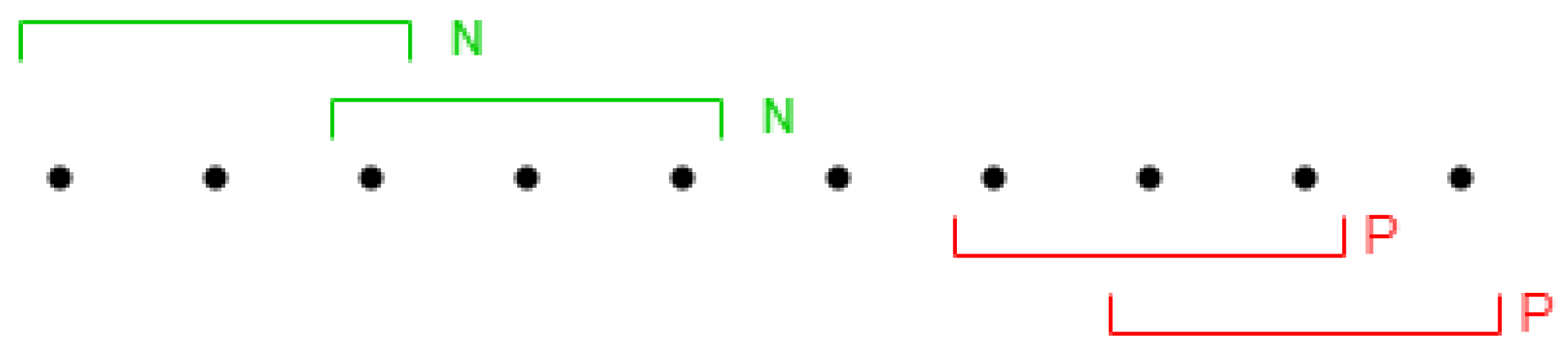
Figure 2.
LSTM Cell. [19]
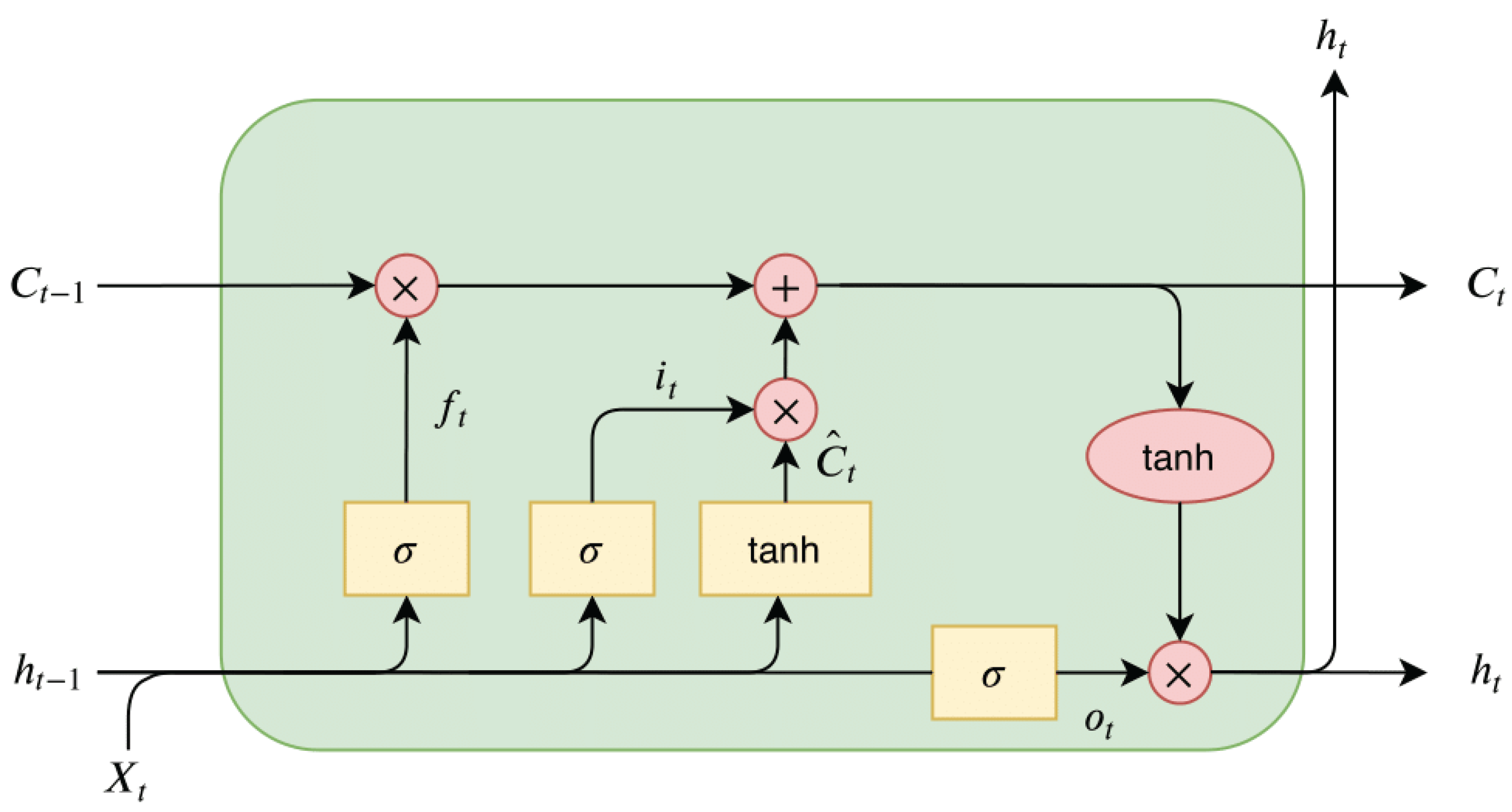
Figure 3.
BiLSTM Architecture. [13]
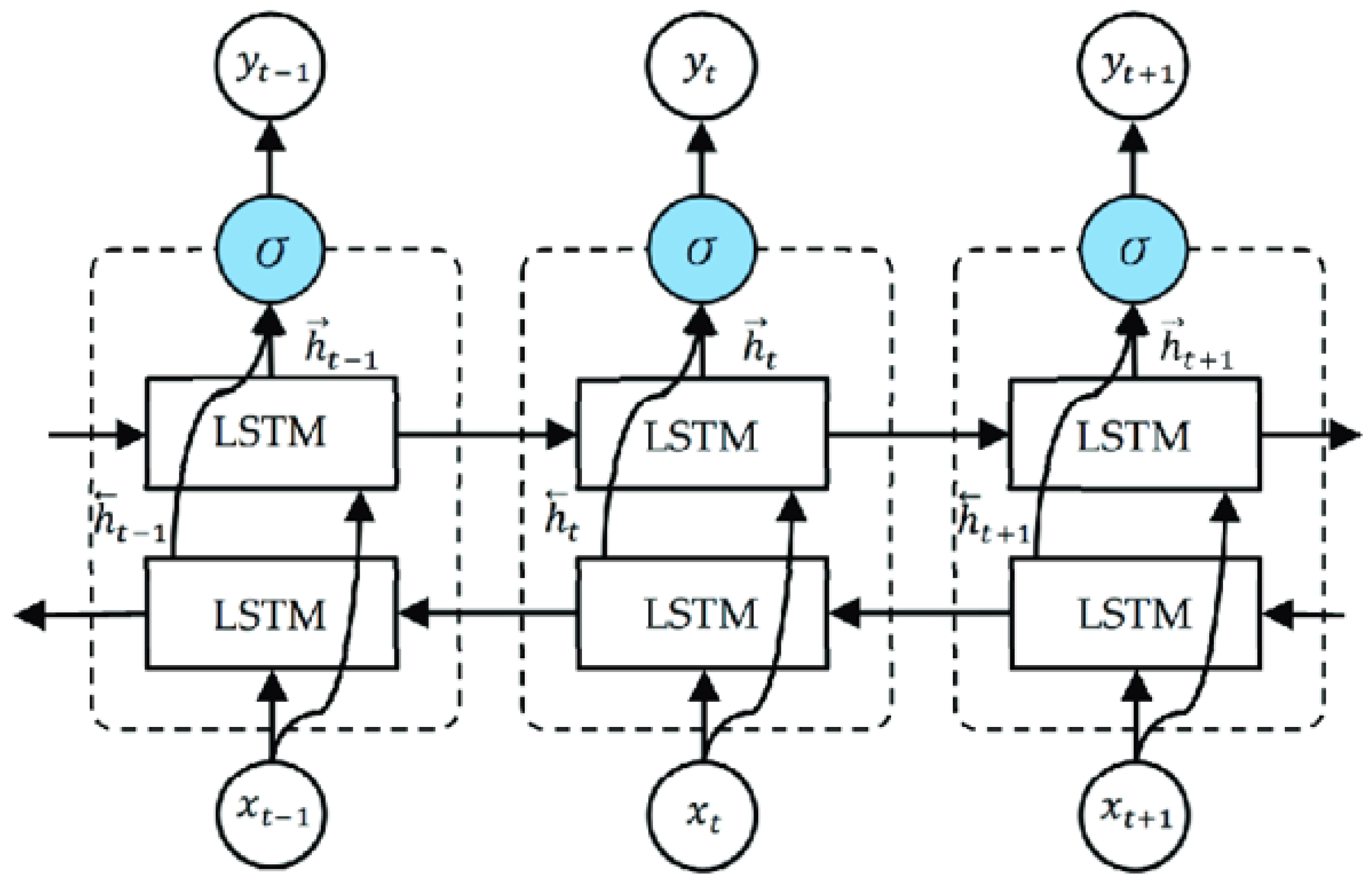
Figure 4.
GRU Cell. [18]
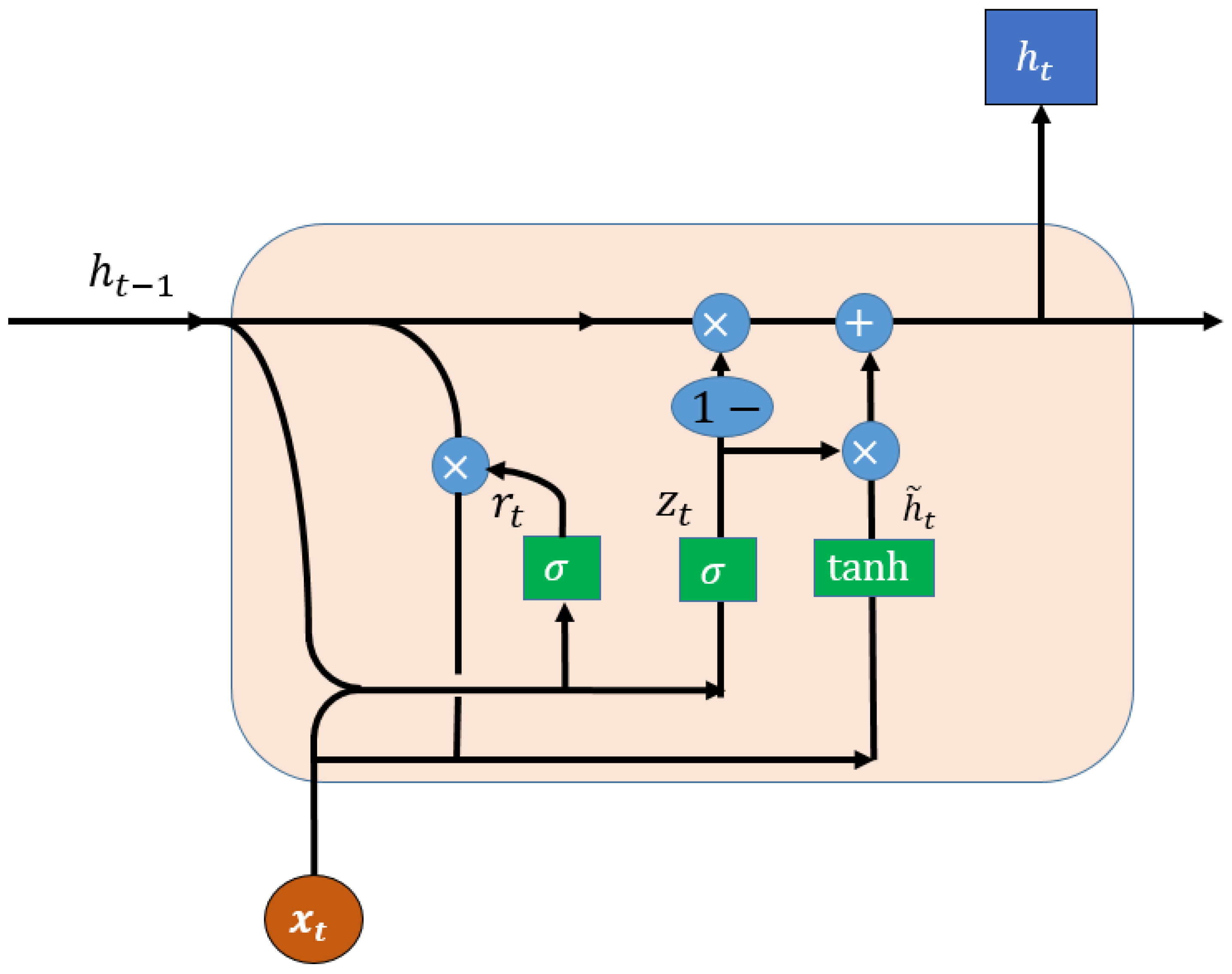
Figure 5.
Accuracy of LSTM Network. In , n and m are the number of layers and units per layer, respectively.
Figure 5.
Accuracy of LSTM Network. In , n and m are the number of layers and units per layer, respectively.
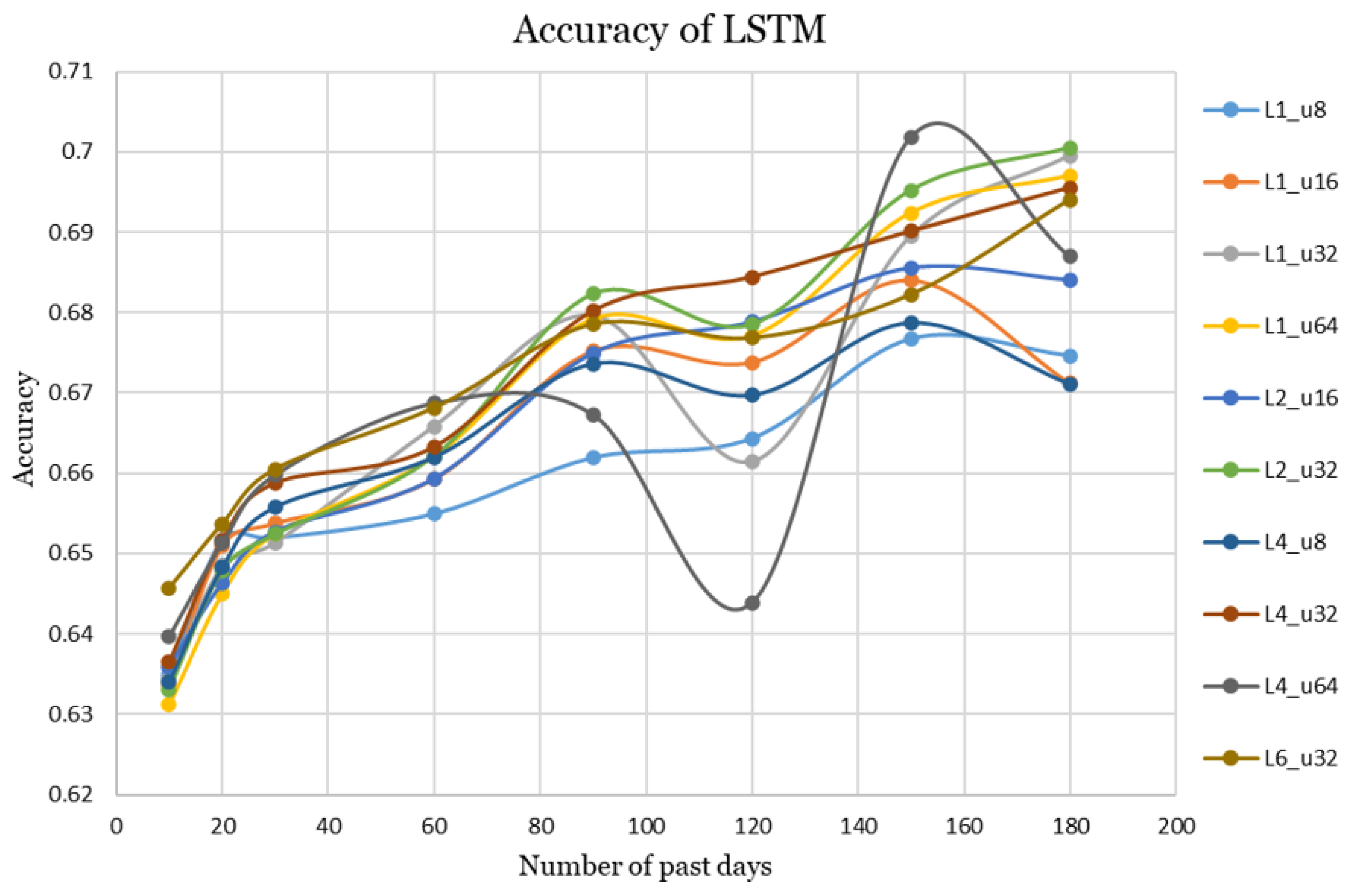
Figure 6.
Accuracy of GRU Network
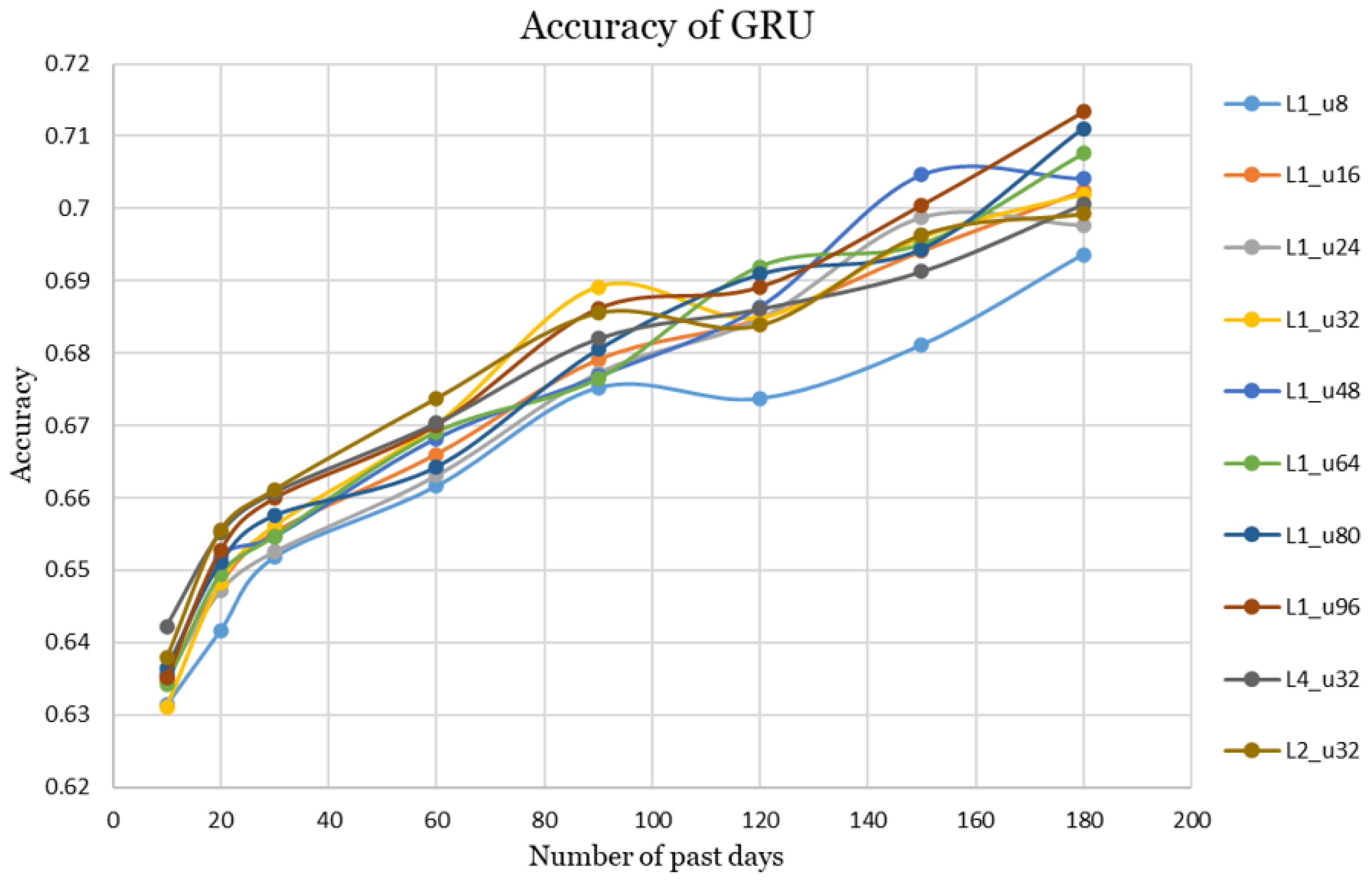
Figure 7.
Accuracy of BiLSTM Network
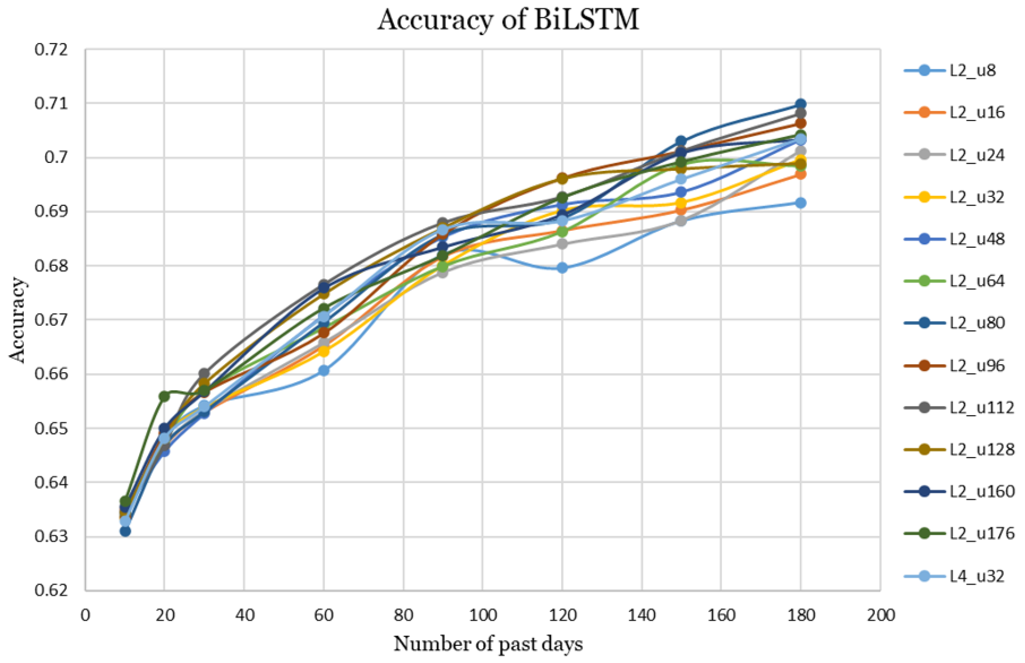
Figure 8.
Final Performance Comparison of LSTM, GRU, and BiLSTM
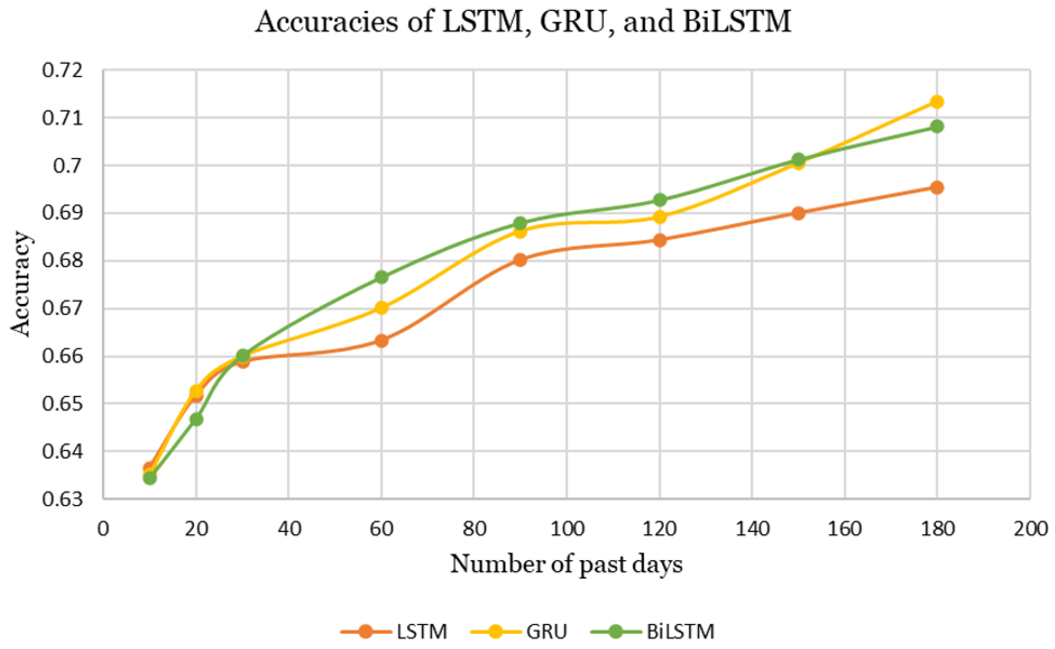

Table 1.
Data size for each experiment (: length of past data, #cryptocurrencies: number of cryptocurrencies with sufficient data, #instances: number of instances created, for ).
Table 1.
Data size for each experiment (: length of past data, #cryptocurrencies: number of cryptocurrencies with sufficient data, #instances: number of instances created, for ).
| 10 | 20 | 30 | 60 | 90 | 120 | 150 | |
|---|---|---|---|---|---|---|---|
| # cryptocurrencies | 4540 | 4338 | 4109 | 3422 | 2904 | 2442 | 2128 |
| # instances | 18160 | 17360 | 16440 | 13700 | 11620 | 9780 | 8520 |
Table 2.
Highest Performing Number of Layer and Unit Combinations of LSTM
| Layers | Units | Past days | F1-Score | Accuracy | Overall AUC |
|---|---|---|---|---|---|
| 1 | 32 | 180 | 0.7345 | 0.6995 | 0.7689 |
| 1 | 64 | 180 | 0.7336 | 0.697 | 0.7679 |
| 2 | 32 | 180 | 0.7358 | 0.7005 | 0.7647 |
| 4 | 64 | 150 | 0.7309 | 0.7018 | 0.7615 |
Table 3.
Highest Performing Number of Layer and Unit Combinations of GRU
| Layers | Units | Past days | F1-Score | Accuracy | Overall AUC |
|---|---|---|---|---|---|
| 1 | 64 | 180 | 0.7391 | 0.7076 | 0.775 |
| 1 | 80 | 180 | 0.7411 | 0.7111 | 0.7779 |
| 1 | 96 | 180 | 0.7438 | 0.7134 | 0.7817 |
| 1 | 128 | 180 | 0.7441 | 0.7087 | 0.7786 |
Table 4.
Highest Performing Number of Layer and Unit Combinations of BiLSTM
| Layers | Units | Past days | F1-Score | Accuracy | Overall AUC |
|---|---|---|---|---|---|
| 2 | 80 | 180 | 0.7427 | 0.7098 | 0.7792 |
| 2 | 96 | 180 | 0.7369 | 0.7063 | 0.7758 |
| 2 | 112 | 180 | 0.7449 | 0.7082 | 0.7801 |
| 2 | 176 | 180 | 0.7397 | 0.7042 | 0.7765 |
Table 5.
Final Performance Comparison of LSTM, GRU, and BiLSTM
| Architecture | Avg_Accuracy | Avg_AUC |
|---|---|---|
| LSTM | 0.6701 | 0.7293 |
| GRU | 0.6759 | 0.7385 |
| BiLSTM | 0.676 | 0.7377 |
Disclaimer/Publisher’s Note: The statements, opinions and data contained in all publications are solely those of the individual author(s) and contributor(s) and not of MDPI and/or the editor(s). MDPI and/or the editor(s) disclaim responsibility for any injury to people or property resulting from any ideas, methods, instructions or products referred to in the content. |
© 2025 by the authors. Licensee MDPI, Basel, Switzerland. This article is an open access article distributed under the terms and conditions of the Creative Commons Attribution (CC BY) license (http://creativecommons.org/licenses/by/4.0/).
Copyright: This open access article is published under a Creative Commons CC BY 4.0 license, which permit the free download, distribution, and reuse, provided that the author and preprint are cited in any reuse.


