Submitted:
04 October 2025
Posted:
06 October 2025
You are already at the latest version
Abstract
Objective: Psoriasis is a chronic, immune-mediated inflammatory disease associated with systemic comorbidities. Detecting subclinical changes in anterior segment parameters related to ocular involvement may be valuable for early diagnosis. This study aimed to classify anterior segment parameters of patients with psoriasis using machine learning (ML) algorithms and interpret them with explainable artificial intelligence (XAI) methods. Methods: Corneal densitometry and anterior segment measurements obtained from 190 participants (106 with psoriasis, 84 controls) using Pentacam HR were analyzed. Imputation of missing values, scaling, and SMOTE balancing were applied during the data preprocessing. Seven ML algorithms (Logistic Regression, SVM-RBF, Random Forest, Gradient Boosting, XGBoost, LightGBM, and CatBoost) were compared. Performance metrics such as accuracy, precision, sensitivity, F1 score, and ROC-AUC were evaluated. Variable importance was determined using SHAP analysis. Results: The best performance was achieved with the CatBoost model (accuracy: 81.4%; F1 = 0.82; ROC-AUC = 0.88). XGBoost and Random Forest ranked second. The SHAP analysis showed that the parameters Z40 (central corneal aberration), posterior densitometry (0–2 mm), and anterior densitometry (6–10 mm) were the most influential variables. Conclusions: Combining ensemble-based ML algorithms, particularly CatBoost, with XAI methods offers a powerful approach for the early and interpretable detection of ocular involvement in patients with psoriasis. This method may contribute to clinical decision support systems.
Keywords:
psoriasis
; anterior segment
; machine learning
; explainable artificial intelligence
; SHAP
1. Introduction
Psoriasis is a chronic, immune-mediated inflammatory disease affecting approximately 2–3% of the global population [1]. While psoriasis vulgaris is the most common form, joint involvement (psoriatic arthritis) and systemic inflammatory processes are also significant causes of morbidity. The etiopathogenesis of the disease is complex; genetic predisposition, immune system dysregulation, and the interaction of environmental factors all play a role in this process. Although psoriasis was long considered solely a dermatological disease, it is now recognized as a systemic inflammatory syndrome. It has been associated with numerous comorbidities, including cardiovascular disease, metabolic syndrome, obesity, diabetes, and gastrointestinal involvement [2].
Among these systemic effects, ocular findings are of particular importance. Although ocular involvement in patients with psoriasis is often overlooked, it is a complication that negatively affects patients’ quality of life. The most commonly reported ocular findings include conjunctivitis, blepharitis, keratoconjunctivitis sicca (dry eye syndrome), and uveitis [3]. Uveitis, in particular, is more common in cases of psoriatic arthritis and can lead to serious vision loss if left untreated. In addition, clinically subtle but subclinical changes in anterior segment parameters are also important indicators of the relationship between psoriasis and the eye [4].
The anterior segment is an anatomical region comprising the cornea, anterior chamber, iris, and lens. Parameters associated with this region include the central corneal thickness, anterior chamber depth (ACD), anterior chamber volume, angle measurements, corneal volume, and high-order aberrations. Inflammatory processes can affect these parameters, causing structural changes in the eye. Today, Scheimpflug-based devices (e.g., Pentacam) allow these parameters to be measured quickly, reliably, and non-invasively [5]. The high-resolution three-dimensional data obtained with Pentacam plays a critical role not only in the evaluation of primary ocular diseases such as keratoconus or glaucoma, but also in demonstrating the subclinical involvement of the eye in systemic inflammatory diseases such as psoriasis.
The rise in artificial intelligence (AI)-based methods in medicine in recent years has ushered in a new era in the development of clinical decision support systems. Artificial intelligence aims to mimic human-like learning and decision-making processes in computers. Machine learning (ML), an important subtopic in this field, offers powerful predictions beyond classical statistical methods owing to its ability to model complex and nonlinear relationships in data [6].
Machine learning methods are primarily categorized into three groups: supervised learning (classification, regression), unsupervised learning (clustering, dimensionality reduction), and reinforcement learning (learning through decision optimization). The most commonly used supervised algorithms in healthcare include Random Forest, Support Vector Machines, Gradient Boosting, XGBoost, LightGBM, and AdaBoost. Ensemble methods, in particular, are widely used in clinical research, providing good classification performance on multivariate and high-dimensional datasets [7,8].
However, despite providing high accuracy, ML models often have a “black box” nature. Knowing which parameters the model is using to make decisions is critically important for clinical applications. This is where explainable artificial intelligence (XAI) comes into play. XAI increases both scientific reliability and clinical applicability by making the decision-making processes of machine learning models transparent. Methods such as SHAP (SHapley Additive exPlanations) and LIME (Local Interpretable Model-agnostic Explanations) contribute to clinicians’ understanding of the results by visualizing the contribution of each parameter to the model. Thus, not only is the result obtained, the variables that led to that result can also be explained.
The use of ML and XAI applications in ophthalmology is increasingly prevalent. Promising results have been obtained in areas such as corneal ectasia detection, glaucoma risk analysis, keratoconus classification, and retinal image analysis [9]. In this context, analyzing anterior segment parameters in patients with psoriasis using ML algorithms and explaining them with XAI methods offers an innovative approach in terms of both increasing the diagnostic accuracy and detecting subclinical involvement at an early stage.
The aim of this study is to classify anterior segment parameters in patients with psoriasis using different machine learning algorithms and explain them using XAI methods. Thus, the goal is to predict ocular involvement at an early stage, provide decision support to clinicians, and lay the groundwork for individualized treatment approaches.
2. Materials and Methods
2.1. Study Design and Data Features
The aim of this study is to classify anterior segment parameters in psoriasis patients using ML methods and develop a prediction model that is integrated with explainable XAI methods. The study used corneal densitometric measurements and anterior segment parameters, obtained with the Scheimpflug imaging system (Pentacam HR) from patients who were diagnosed with psoriasis and visited the eye clinic at Sivas Cumhuriyet University Health Services Application and Research Hospital between 2021 and 2022. The mean age of the patients included in the study was 35.75 ± 13.32, while that of the control group was 33.99 ± 10.187. The dataset consisted of 106 observations (55.8%) in the psoriasis group and 84 observations (44.2%) in the control group. Since this created a slight imbalance between the classes, the Synthetic Minority Over-sampling Technique (SMOTE) was applied to the training data to enable the model to learn independently of the class distribution. SMOTE increased the number of examples in the control group from 84 to 106, balancing both classes. Table 1 shows the input and output factors/features used in the analysis.
2.2. ML and XAI Approaches
In this study, the data was stratified into 80% for training and 20% for testing. Missing values in numerical variables were imputed using the median and scaled using StandardScaler. Feature selection was performed on the training data using the SelectFromModel method based on Random Forest (n_estimators = 500), selecting variables above the median importance threshold. Since this step was implemented within the pipeline, there was no information leakage to the test data.
Seven different algorithms were evaluated during the modeling process: Logistic Regression (LR), Random Forest (RF), Gradient Boosting, Radial Basis Function kernel-based Support Vector Machine (SVM), Extreme Gradient Boosting (XGBoost), Light Gradient Boosting Machine (LightGBM), and Categorical Boosting (CatBoost). All models were trained using the same preprocessing and feature selection pipeline, and performance comparisons were only made of the test data. Model selection was based on test results, with the priority order set as accuracy > F1 > ROC-AUC. Accuracy, precision, recall, and F1 scores were calculated, and ROC-AUC values were reported based on probability predictions.
During the explainability phase, SHapley Additive Explanations (SHAP) analyses were performed for the model showing the best performance on the test data. TreeExplainer was used for tree-based models, LinearExplainer for Logistic Regression, and KernelExplainer for other methods such as SVM-RBF. The background matrix was created using features selected from the training data, while the evaluation matrix was created using features selected from the test data. Global variable importance rankings were determined using SHAP analyses and visualized using bar and beeswarm plots. With this approach, a balanced and explainable ML model was developed for the classification of anterior segment parameters in psoriasis patients. Ten-fold cross-validation (CV) was used to evaluate models predicting psoriasis patients. CV, a technique used to measure the generalizability of an ML model to unseen data, involves splitting the dataset into folds, training the model on a subset, and evaluating it on the remainder. In 10-fold CV, the dataset is divided into 10 equal parts, each part is used once for evaluation, and the remaining parts are used for training 10 times. This provides a robust assessment of the model’s performance and reduces variability in performance estimates [10,11].
2.3. Statistical Methods
This study, a range of Python (version 3.11.9) packages was employed to conduct machine learning and explainability (XAI) procedures. Data preprocessing and organization were performed using Pandas and NumPy. The Scikit-learn library was utilized to construct machine learning models, perform feature selection (SelectFromModel), preprocess data (StandardScaler, SimpleImputer, ColumnTransformer, Pipeline), and evaluate model performance metrics. The algorithms implemented included Logistic Regression, Random Forest, Gradient Boosting, Support Vector Classification (SVC), XGBoost, LightGBM, and CatBoost. The Joblib package was used to store model outputs, while matplotlib.pyplot supported visualization. Furthermore, the SHAP (SHapley Additive Explanations) library was applied to interpret model predictions and quantify feature importance
2.4. Categorical Boosting (CatBoost)
CatBoost is a machine learning approach that works with both categorical and numerical data. It stands out for its ability to reduce overfitting by eliminating noise points. This is achieved by adding previous values to areas with low-frequency features and high density. The approach is based on gradient-boosted decision trees. CatBoost overcomes the bias and prediction value drift of the gradient descent technique to correctly interpret data and analyze results. CatBoost comes in both CPU and GPU versions. In communities of equivalent size, the GSU application outperforms both state-of-the-art open-source GBDT GSU applications and XGBoost and LightGBM, enabling much faster training. The package also includes a fast CPU scoring application that outperforms XGBoost and LightGBM in communities of a similar size. CatBoost, in particular, excels at handling categorical features without the need for preprocessing and instantly converts original categories into numerical values. Noise points in models with overfitting are reduced by adding a previous value at low-frequency and high-density points. This improves the model’s generalization while reducing overfitting [12,13].
2.5. Extreme Gradient Boosting (XGBoost)
Chen and Guestrin created the XGBoost algorithm, an advanced Gradient Boosting approach that is similar to GB decision trees and machines. XGBoost is an advanced machine learning algorithm that is part of the ensemble learning technique family and built on the Gradient Boosting framework. In this method, a series of decision trees are created, each attempting to correct the errors of the previous one. It features regularization to prevent overfitting and parallelization during tree creation, allowing for parallel computation. Due to these features, it is a great candidate for large-scale datasets, offering much faster performance than many alternative implementations. Despite its advantages, XGBoost can be prone to overfitting if not properly tuned, especially when dealing with noisy data [14].
2.6. Random Forest (RF)
Random Forest enhances a model’s robustness by creating multiple decision trees for prediction, making the results more reliable. Each decision tree contains a unique set of features and training examples, making it useful for various prediction and classification applications. RF consists of numerous decision trees, each created with different data and features. It is incredibly accurate and robust, minimizes the likelihood of overfitting, and is more adaptable to multi-feature datasets and high-dimensional feature data [15].
2.7. Light Gradient Boosting Machine (LightGBM)
Microsoft introduced LightGBM, a data model based on Gradient Boosting decision trees (GBDTs), in 2017 [16]. Like previous development models, GBDT also converts weak learners into strong ones. LightGBM primarily uses an updated histogram method to enhance the computational power and accuracy of the predictive model. One-dimensional features are divided into several representative bins. The resulting bins are then combined to form a histogram. Each bin in the histogram has two types of data: gradient and total occurrence count. LightGBM scans multiple line graphs to determine the optimal segmentation point for nodes in multidimensional datasets. This model performs better than the GBDT method in terms of training time and space efficiency [17].
2.8. Gradient Boosting (GB)
Gradient Boosting (GB) is a supervised learning system that uses ensemble methods to build successive models to maximize a specific objective function. At each step, the technique attempts to reduce prediction errors by iteratively fitting weak learners—typically decision trees—to the residual errors of the current model. This iterative procedure aims to gradually improve the model’s performance, as detailed in [18]. The objective is to minimize a defined loss function by combining weak learners using an additive method. The procedure begins with the initialization of the model. The initial model F0(x) is formulated to minimize empirical risk and is expressed as follows:
In this equation, yi is the target value of the i-th data point, and c is a constant used to initialize the model. For regression tasks, the loss function L measures the difference between the predicted and actual values, in a similar way to the mean squared error. The total number of data points in the dataset is represented by N.
2.9. Support Vector Machine (SVM–Radial Basis Function (RBF))
Support Vector Machines (SVMs) are machine learning models that are commonly used for regression and classification. The main goal is to define a hyperplane that effectively separates the classes of the target variable. To achieve this, an SVM uses a kernel technique that transforms the data into a higher-dimensional space to discover the best decision boundary. Kernel-based techniques initially perform these complex transformations without first determining how the data should be effectively partitioned based on labels or outcomes. This feature leads to SVMs becoming massive datasets [19,20].
2.10. Logistic Regression (LR)
First proposed by Cox in the mid-20th century, Logistic Regression is one of the most widely used statistical procedures for evaluating binary outcomes such as “yes/no,” “dead/alive,” or “successful/unsuccessful.” In education research, Logistic Regression helps determine how student and teaching factors predict a specific educational outcome [21,22], while clinical risk prediction models typically calculate the likelihood of a diagnosis or health outcome based on specific factors. These approaches facilitate collaborative decision-making in medicine. They use individual-level data to assess the likelihood of diagnosis, disease progression, or outcomes. Traditionally, they are created using regression models such as LR, for which ML techniques are becoming increasingly popular. LR is a generalized linear model that explains or predicts the relationship between a categorical outcome variable and one or more predictors [23,24].
2.11. SHapley Contribution Explanations (SHAP)
An algorithm defines how data elements, features, or variables contribute to predictions or models. Machine learning is a subfield of artificial intelligence that uses algorithms to make accurate predictions or models without requiring explicit programming. Machine learning algorithms utilize statistical analysis to predict outcomes and update them as new data becomes available [25]. SHAP uses game theory principles to provide local explanations for the model’s predictions [26]. In game theory, the model represents the rules of the game, while the input features represent potential players who may participate in the game (observed features) or not (unobserved features). As a result, the SHAP technique calculates Shapley values by testing the model with various combinations of input features and calculating the average difference in the output (prediction) when a feature is present and when it is absent. This difference, known as the Shapley value, indicates the feature’s contribution to the model’s expected value. Consequently, Shapley values determine each feature’s contribution to the model’s prediction for a given input [27].
2.12. Confusion Matrix
A confusion matrix summarizes a classifier’s actual and predicted classifications. Performance is typically evaluated using the following metrics derived from the matrix: true positives (TPs), true negatives (TNs), false positives (FPs), and false negatives (FNs) [28].
2.13. Model Evaluation Metrics
Accuracy (ACC): Accuracy represents the ratio of correctly classified examples across all classes relative to the total number of predictions. It reflects the overall classification ability of the trained model [29].
Precision (PREC): Precision is defined as the ratio of true positive predictions among all examples that were classified as positive by the model [30].
Recall (Sensitivity): Recall measures the model’s ability to correctly identify true positive cases among all true positives. In other words, it represents the probability that a sample belonging to the positive class will be correctly recognized by the model [31].
F1 Score: The F1 score is the harmonic mean of precision and recall. This metric provides a balanced evaluation by including both false positives and false negatives [32].
AUC-ROC: The area under the receiver operating characteristic curve (AUC-ROC) is a reliable metric for evaluating a model’s discriminative capacity across different threshold levels. The ROC curve illustrates the relationship between sensitivity (true positive rate) and 1-specificity (false positive rate). A high AUC value indicates advanced discrimination ability; values close to 1.0 indicate exceptional classification adequacy, while values close to 0.5 indicate performance that is similar to chance [33].
3. Results
Seven different machine learning algorithms were compared in this study, and their accuracy, precision, recall, F1 score, and ROC-AUC performance are summarized in Table 2.
The CatBoost and XGBoost models achieved the highest accuracy rate (0.8140). The CatBoost model also had the highest F1 score (0.8182) and the highest ROC-AUC value (0.8766). The XGBoost model showed the highest precision (0.8824) value. The Random Forest model ranked third, with an accuracy of 0.7907 and an ROC-AUC of 0.8593. The LightGBM (0.7674 accuracy, 0.8074 ROC-AUC) and Gradient Boosting (0.7442 accuracy, 0.8074 ROC-AUC) models showed moderate performance. The SVM (RBF) model showed lower performance, with an accuracy of 0.6744 and an ROC-AUC of 0.7554. The lowest performance was observed for the Logistic Regression model (0.6279 accuracy, 0.6082 ROC-AUC).
The SHAP analysis performed for the CatBoost model determined the contribution levels of the variables to the model. The highest contribution was observed from the Z40 (central) variable (0.246), followed by Posterior CD 0–2 mm (GSU) (0.181) and Anterior CD 6–10 mm (GSU) (0.169). Medium contributions were observed from corneal volume (CoV) (0.149), flat keratometry (K1) (0.138), thinnest corneal thickness (CT) (0.136), central CD 0–2 mm (GSU) (0.136), anterior chamber volume (ACV) (0.128), vertical keratometry (K2) (0.117), and anterior chamber angle (ACA) (0.112). Smaller contributions were found for the variables Z40 (back) (0.099), Posterior Total (0–12 mm) (0.092), Z40 (front) (0.086), and anterior chamber depth (ACD) (0.079), while the variables making the smallest contributions were Posterior CD 2–6 mm (GSU) (0.078), Anterior CD (0–12 mm GSU) (0.061), total thickness (6–10) (0.052), Center Total (0–12 mm GSU) (0.052), RMS HOAs (central) (0.042), and RMS HOAs (front) (0.042). These results are summarized in Table 3.

Table 3.
Test performance of machine learning algorithms.
| Model | Accuracy | Precision | Recall | F1 Score | ROC-AUC |
|---|---|---|---|---|---|
| CatBoost | 0.8140 | 0.7826 | 0.8571 | 0.8182 | 0.8766 |
| XGBoost | 0.8140 | 0.8824 | 0.7143 | 0.7895 | 0.8377 |
| Random Forest | 0.7907 | 0.7727 | 0.8095 | 0.7907 | 0.8593 |
| LightGBM | 0.7674 | 0.7895 | 0.7143 | 0.7500 | 0.8074 |
| Gradient Boosting | 0.7442 | 0.7500 | 0.7143 | 0.7317 | 0.8074 |
| SVM (RBF) | 0.6744 | 0.6522 | 0.7143 | 0.6818 | 0.7554 |
| Logistic Regression | 0.6279 | 0.6316 | 0.5714 | 0.6000 | 0.6082 |
Table 4.
Importance ranking of variables based on SHAP analysis.
| Feature | Shap | |
|---|---|---|
| 0 | Z40(central) | 0.246204 |
| 1 | Posterior CD 0–2 mm (GSU) | 0.181423 |
| 2 | Anterior CD 6–10 mm (GSU) | 0.169333 |
| 3 | CoV | 0.149440 |
| 4 | K1 | 0.138394 |
| 5 | CT | 0.136007 |
| 6 | Central CD 0–2 mm (GSU) | 0.135759 |
| 7 | ACV | 0.127746 |
| 8 | K2 | 0.116788 |
| 9 | ACA | 0.111780 |
| 10 | Z40 (back) | 0.098672 |
| 11 | Posterior Total (0–12) mm (GSU) | 0.091918 |
| 12 | Z40 (front) | 0.086212 |
| 13 | ACD | 0.078599 |
| 14 | Posterior CD2–6 mm (GSU) | 0.077908 |
| 15 | Anterior CD (0–12) mm (GSU) | 0.060916 |
| 16 | Total thickness (6–10) | 0.052341 |
| 17 | Center Total (0–12) mm (GSU) | 0.051937 |
| 18 | RMS HOAs (central) | 0.042040 |
| 19 | RMS HOAs (front) | 0.041783 |
Figure 1 shows that the most decisive variable in the model’s decision-making process is Z40 (central). It is followed by Posterior CD 0–2 mm (GSU) and Anterior CD 6–10 mm (GSU), respectively. Variables contributing at a moderate level include corneal volume (CoV), keratometry values (K1, K2), thinnest corneal thickness (CT), central CD 0–2 mm, and anterior chamber parameters (ACV, ACA). More limited effects were observed for the Z40 (back/front), Posterior Total (0–12 mm), and anterior chamber depth (ACD) parameters. The lowest contribution was found to be associated with posterior and anterior total measurements, total thickness (6–10), and high-order aberrations (RMS HOAs, central/front
The summary of the SHAP analysis revealed that the variable with the highest contribution in the CatBoost model was Z40 (central). This was followed by Posterior CD 0–2 mm (GSU), Anterior CD 6–10 mm (GSU), CoV, K1, CT, central CD 0–2 mm (GSU), ACV, K2, and ACA. Variables making moderate contributions included Z40 (back), Posterior Total (0–12 mm) (GSU), Z40 (front), and ACD. Variables making smaller contributions were determined to be Posterior CD 2–6 mm (GSU), Anterior CD (0–12 mm) (GSU), total thickness (6–10), Center Total (0–12 mm) (GSU), RMS HOAs (central), and RMS HOAs (front).
Figure 2 shows the performance of the seven different classification models on the test set, evaluated using ROC curves. The LR model achieved the lowest AUC value (0.61) for differentiating between psoriasis patients and the control group. The CatBoost (0.88), Random Forest (0.86), and XGBoost (0.84) models, on the other hand, exhibited the highest AUC values, while LightGBM (0.81), Gradient Boosting (0.81), and SVM (0.76) showed moderate efficacy in differentiating psoriasis patients from the control group. Overall, the graph demonstrates that tree-based approaches outperform the linear model. The CatBoost model (0.88) was shown to be more effective than the other techniques in differentiating between psoriasis sufferers and control subjects.
4. Discussion and Conclusions
This study evaluated the performance of machine learning algorithms in classifying anterior segment parameters of psoriasis patients. The results indicate that tree-based methods, in particular, stand out. CatBoost was the most successful model, achieving 81% accuracy, 86% sensitivity, and 88% ROC-AUC. This finding reveals that this algorithm not only offers high classification success but also a significant advantage in correctly identifying affected individuals.
The XGBoost model achieved a similar accuracy rate (81%); however, despite its high precision (88%), its low sensitivity (71%) indicates that this model is effective in reducing false positives but more limited in capturing patients. Random Forest, on the other hand, stood out as a reliable alternative, demonstrating a balanced performance with 79% accuracy and 86% ROC-AUC. LightGBM (77% accuracy) and Gradient Boosting (74% accuracy), which showed moderate performance, were advantageous in terms of speed and efficiency but lagged behind CatBoost and XGBoost in terms of clinical sensitivity. Among the classical methods, SVM (RBF kernel) achieved 67% accuracy, while Logistic Regression achieved 63% accuracy and 61% ROC-AUC, representing the lowest performance values; this result indicates that linear methods are limited in heterogeneous and complex datasets such as ones involving psoriasis.
Compared with the literature, our findings are generally consistent. Indeed, as noted in the study by Yu et al. (2018), tree-based and deep learning-based methods provide higher accuracy for clinical data [34]. Dong et al. (2021) reported ROC-AUC values ranging from 0.85 to 0.89 when predicting acute kidney injury in pediatric intensive care patients using a community-based model [35]. Similarly, Cao et al. (2021) used Random Forest to detect subclinical keratoconus and achieved 98% accuracy, 97% sensitivity, and 98% specificity [36]. These findings support the current results and highlight the power of ensemble models in biomedical data analysis. On the other hand, while LightGBM and Gradient Boosting showed moderate performance with an ROC-AUC value of 0.8074, SVM (RBF) and Logistic Regression showed the lowest classification success, indicating that linear or kernel-based approaches are insufficient for modeling complex and nonlinear biomedical datasets. Previous studies have also highlighted that classical statistical models such as Logistic Regression are limited in capturing complex biological interactions, while machine learning approaches provide superior predictive power [37]. Overall, the findings of this study, consistent with the existing literature, demonstrate that reinforcement and community-based methods are more robust and clinically applicable in biomedical data analysis. CatBoost minimizes the risk of missing patient cases with its high sensitivity; XGBoost reduces false alarms with its high sensitivity; and Random Forest provides a balanced and stable performance. In contrast, simpler models such as Logistic Regression and SVM fail to meet clinical accuracy requirements, confirming that advanced ensemble models are more suitable for real-world biomedical applications.
SHAP analysis has made the decision-making processes of models more transparent, revealing which parameters play a decisive role in classification. According to our analysis results, Z40 (central)—the central corneal aberration value—has the strongest influence, showing that it is the most powerful predictor in distinguishing psoriasis from the control group. This finding suggests that central corneal optical aberrations may be closely related to the disease.
Second in importance is Posterior CD 0–2 mm (GSU)—the densitometer measurement in the 0–2 mm zone of the posterior corneal layer—which contributes significantly to the classification power of structural changes in the posterior corneal layer.
Third is the Anterior CD 6–10 mm (GSU)—the densitometer measurement in the 6–10 mm zone of the anterior layer of the cornea—showing that the mid-peripheral region of the anterior corneal structure also plays a critical role in disease differentiation.
In addition, parameters such as the corneal volume (CoV), flat keratometry (K1), thinnest corneal thickness (CT), anterior chamber volume (ACV), vertical keratometry (K2), and anterior chamber angle (ACA) provide moderate contributions, suggesting that both the corneal thickness and anterior segment geometry reflect structural differences associated with psoriasis. Variables making lower contributions included the anterior chamber depth (ACD), Posterior Total average densitometer value (Posterior Total 0–12 mm GSU), and anterior/posterior surface corneal aberration values (Z40 front/back). Although these parameters contributed to classification at a secondary level, they are biologically meaningful, as they represent different aspects of corneal integrity.
4.1. Strengths and Limitations of the Study
One of the strengths of this research is the use of current machine learning techniques and the systematic comparison of different algorithms. By precisely calculating the degree to which each feature in the model contributes to the prediction results using SHAP analysis, a high degree of interpretability of the machine learning models is achieved. This approach represents an important step toward a more objective assessment of ophthalmic findings in patients with psoriasis. However, there are some limitations. First, the data used in the study are cross-sectional, and the change in anterior segment findings over time or the response to treatment in patients with psoriasis has not been evaluated. Additionally, validation studies with multicenter and larger samples are needed.
4.2. Conclusions and Future Perspectives
The classification of anterior segment parameters in psoriasis patients using machine learning and the identification of the variables contributing the most to the model through SHAP analysis represent important findings from a diagnostic and prognostic perspective. This study demonstrates that this approach is technically feasible and can offer valuable contributions to clinical practice. However, the establishment of standardized protocols, independent validation studies, and multicenter collaborations are of great importance for the transition to clinical use.
Rapid technological advances and increasing data diversity pave the way for the development of more reliable and sophisticated models in the future. Such models are expected to play an important role in the early detection of ophthalmological complications in psoriasis patients, the objective assessment of disease severity, and the development of personalized treatment strategies.
Furthermore, an interdisciplinary approach is critical for ensuring the sustainability of progress in this field. Consequently, machine learning algorithms can be considered not only as technical classification tools but also as powerful aids supporting clinical decision-making processes. When used in conjunction with explainable artificial intelligence (XAI) methods, the transparency provided by these models increases clinician confidence and holds promise for their integration into more widespread clinical applications in the future. The use of these approaches in the early diagnosis of ophthalmic complications associated with psoriasis, such as dry eye, will be an important step toward directly improving patients’ quality of life.
Funding
This research received no external funding
Data Availability Statement
The study was conducted in accordance with the ethical principles stated in the Declaration of Helsinki. The study protocol was approved by Sivas Cumhuriyet University health sciences research ethics committee (decision no:2025-07/66, date: 31.07.2025).
Conflicts of Interest
The authors declare no conflicts of interest.
References
- Kang, Z.; Zhang, X.; Du, Y.; Dai, S.-M. Global and regional epidemiology of psoriatic arthritis in patients with psoriasis: A comprehensive systematic analysis and modeling study. J. Autoimmun. 2024, 145, 103202. [Google Scholar] [CrossRef]
- Karadag, A.S.; Bilgili, S.G.; Çalka, Ö.; Demircan, Y.T. Retrospective Evaluation of Childhood Psoriasis Clinically and Demographic Features. Turk. J. Dermatol. 2013, 7, 13. [Google Scholar] [CrossRef]
- Valdés-Arias, D.; Locatelli, E.V.; Sepulveda-Beltran, P.A.; Mangwani-Mordani, S.; Navia, J.C.; Galor, A. Recent United States developments in the pharmacological treatment of dry eye disease. Drugs 2024, 84, 549–563. [Google Scholar] [CrossRef]
- Gontarz, K.; Dorecka, M.; Mrukwa-Kominek, E. Psoriasis and the eyelids and ocular surface—A current review of the literature. Ophthalmology 2023, 2023, 41–43. [Google Scholar] [CrossRef]
- Youssef, A.R.; Sharawy, A.; Shebl, A.A. Comparison of Anterior Segment Optical Coherence Tomography and Pentacam in the Diagnosis of Keratoconus. Benha Med. J. 2025, 42, 69–78. [Google Scholar] [CrossRef]
- Han, J.; Pei, J.; Tong, H. Data Mining: Concepts and Techniques;Morgan Kaufmann 2022.
- Schonlau, M.; Zou, R.Y. The random forest algorithm for statistical learning. Stata J. 2020, 20, 3–29. [Google Scholar] [CrossRef]
- Lu, C.; Guan, Y.; van Lieshout, M.-C.; Xu, G. XGBoostPP: Tree-based estimation of point process intensity functions. J. Comput. Graph. Stat. 2025., 1–12. [CrossRef]
- Madadi, Y.; Delsoz, M.; Khouri, A.S.; Boland, M.; Grzybowski, A.; Yousefi, S. Applications of artificial intelligence-enabled robots and chatbots in ophthalmology: Recent advances and future trends. Curr. Opin. Ophthalmol. 2024, 35, 238–243. [Google Scholar] [CrossRef]
- Yagin, F.H.; Cicek, I.B.; Alkhateeb, A.; Yagin, B.; Colak, C.; Azzeh, M.; Akbulut, S. Explainable artificial intelligence model for identifying COVID-19 gene biomarkers. Comput. Biol. Med. 2023, 154, 106619. [Google Scholar] [CrossRef]
- Macin, G.; Tasci, B.; Tasci, I.; Faust, O.; Barua, P.D.; Dogan, S.; Tuncer, T.; Tan, R.-S.; Acharya, U.R. An accurate multiple sclerosis detection model based on exemplar multiple parameters local phase quantization: ExMPLPQ. Appl. Sci. 2022, 12, 4920. [Google Scholar] [CrossRef]
- Prokhorenkova, L.; Gusev, G.; Vorobev, A.; Dorogush, A.V.; Gulin, A. CatBoost: Unbiased boosting with categorical features. In Advances in Neural Information Processing Systems; 2018; Volume 31.
- Dorogush, A.V.; Ershov, V.; Gulin, A. CatBoost: Gradient boosting with categorical features support. arXiv 2018, arXiv:181011363.
- Chen, T.; Guestrin, C. (Eds) Xgboost: A scalable tree boosting system. In Proceedings of the 22nd ACM SIGKDD International Conference on Knowledge Discovery and Data Mining, San Francisco, CA, USA, 13–17 August 2016. [Google Scholar] [CrossRef]
- Luo, D.; Qiao, X. Regional agricultural drought vulnerability prediction based on interpretable Random Forest. Environ. Monit. Assess. 2024, 196, 1123. [Google Scholar] [CrossRef]
- Li, K.; Xu, H.; Liu, X. Analysis and visualization of accident severity based on LightGBM-TPE. Chaos Solitons Fractals 2022, 157, 111987. [Google Scholar] [CrossRef]
- Liu, S.; Sun, Y.; Zhang, L.; Su, P. Fault diagnosis of shipboard medium-voltage DC power system based on machine learning. Int. J. Electr. Power Energy Syst. 2021, 124, 106399. [Google Scholar] [CrossRef]
- Kim, C.; Park, T. Predicting determinants of lifelong learning intention using gradient boosting machine (GBM) with grid search. Sustainability 2022, 14, 5256. [Google Scholar] [CrossRef]
- Xu, W.; Zhang, J.; Zhang, Q.; Wei, X. (Eds) Risk prediction of type II diabetes based on random forest model. In Proceedings of the 2017 Third International Conference on Advances in Electrical Electronics Information Communication Bio-Informatics, Chennai, India, 27–28 February 2017; IEEE: Piscataway,NJ,USA, 2017. [Google Scholar] [CrossRef]
- Yang, Q.; Li, Y.; Li, B.; Gong, Y. A novel multi-class classification model for schizophrenia, bipolar disorder and healthy controls using comprehensive transcriptomic data. Comput. Biol. Med. 2022, 148, 105956. [Google Scholar] [CrossRef]
- Cox, D.R. The regression analysis of binary sequences. J. R. Stat. Soc. Ser. B Stat. Methodol. 1958, 20, 215–232. [Google Scholar] [CrossRef]
- Cramer, J.S. The Origins of Logistic Regression; Tinbergen Institute discussion paper; 2002. [CrossRef]
- Moons, K.G.M.; Altman, D.G.; Reitsma, J.B.; Ioannidis, J.P.A.; Macaskill, P.; Steyerberg, E.W.; Vickers, A.J.; Ransohoff, D.F.; Collins, G.S. Transparent Reporting of a multivariable prediction model for Individual Prognosis or Diagnosis (TRIPOD): Explanation and elaboration. Ann. Intern. Med. 2015, 162, W1–W73. [Google Scholar] [CrossRef]
- Shalev-Shwartz, S.; Ben-David, S. Understanding Machine Learning: From Theory to Algorithms; Cambridge University Press: Cambridge, UK, 2014. [Google Scholar] [CrossRef]
- Mihirette, S.; Tan, Q. Classification. In International Conference on Hybrid Artificial Intelligence Systems; Springer: Berlin/ Heidelberg, Germany, 2022. [Google Scholar] [CrossRef]
- Chen, H. Catboost Model Unveiled; 2025; pp. 14–48(35). [CrossRef]
- Alabi, R.O.; Almangush, A.; Elmusrati, M.; Leivo, I.; Mäkitie, A.A. An interpretable machine learning prognostic system for risk stratification in oropharyngeal cancer. Int. J. Med. Inform. 2022, 168, 104896. [Google Scholar] [CrossRef]
- Ibrahim, A.A.; Ridwan, R.L.; Muhammed, M.M.; Abdulaziz, R.; Saheed, G.A. Comparison of the CatBoost Classifier with other Machine Learning Methods. Int. J. Adv. Comput. Sci. Appl. 2020, 11. [Google Scholar] [CrossRef]
- Liddle, A.R.; Mukherjee, P.; Parkinson, D. Model Selection and Multi-Model Inference; Cambridge University Press: Cambridge, UK, 2009; pp. 79–98. [Google Scholar] [CrossRef]
- Müller, A.C.; Guido, S. Introduction to Machine Learning with Python: A Guide for Data Scientists; O’Reilly Media, Inc.: Sebastopol, CA, USA, 2016. [Google Scholar]
- Japkowicz, N.; Shah, M. Evaluating Learning Algorithms: A Classification Perspective; Cambridge University Press: Cambridge, UK, 2011. [Google Scholar] [CrossRef]
- Güneş, S.; Polat, K.; Yosunkaya, Ş. Multi-class f-score feature selection approach to classification of obstructive sleep apnea syndrome. Expert Syst. Appl. 2010, 37, 998–1004. [Google Scholar] [CrossRef]
- Stern, R.H. Interpretation of the area under the ROC curve for risk prediction models. arXiv 2021, arXiv:2102.11053. [Google Scholar] [CrossRef]
- Yu, K.H.; Beam, A.L.; Kohane, I.S. Artificial intelligence in healthcare. Nat. Biomed. Eng. 2018, 2, 719–731. [Google Scholar] [CrossRef]
- Dong, J.; Feng, T.; Thapa-Chhetry, B.; Cho, B.G.; Shum, T.; Inwald, D.P.; Newth, C.J.L.; Vaidya, V.U. Machine learning model for early prediction of acute kidney injury in pediatric critical care. Crit Care 2021, 25, 288. [Google Scholar] [CrossRef] [PubMed]
- Cao, K.; Verspoor, K.; Chan, E.; Daniell, M.; Sahebjada, S.; Baird, P.N. Machine learning with a reduced dimensionality representation of comprehensive Pentacam tomography parameters to identify subclinical keratoconus. Comput. Biol. Med. 2021, 138, 104884. [Google Scholar] [CrossRef] [PubMed]
- Kaur, I.; Doja, M.; Ahmad, T. Data mining and machine learning in cancer survival research: An overview and future recommendations. J. Biomed. Inform. 2022, 128, 104026. [Google Scholar] [CrossRef] [PubMed]
Figure 1.
CatBoost model interpretation. (A) SHAP beeswarm plot illustrating the relevance of the top 20 Pentacam parameters regarding their stability and interpretability. (B) SHAP bar plot displaying the mean order of importance of the same 20 parameters (|SHAP value|); higher SHAP values indicate a stronger contribution of a feature to classifying patients into the psoriasis group rather than the control group.
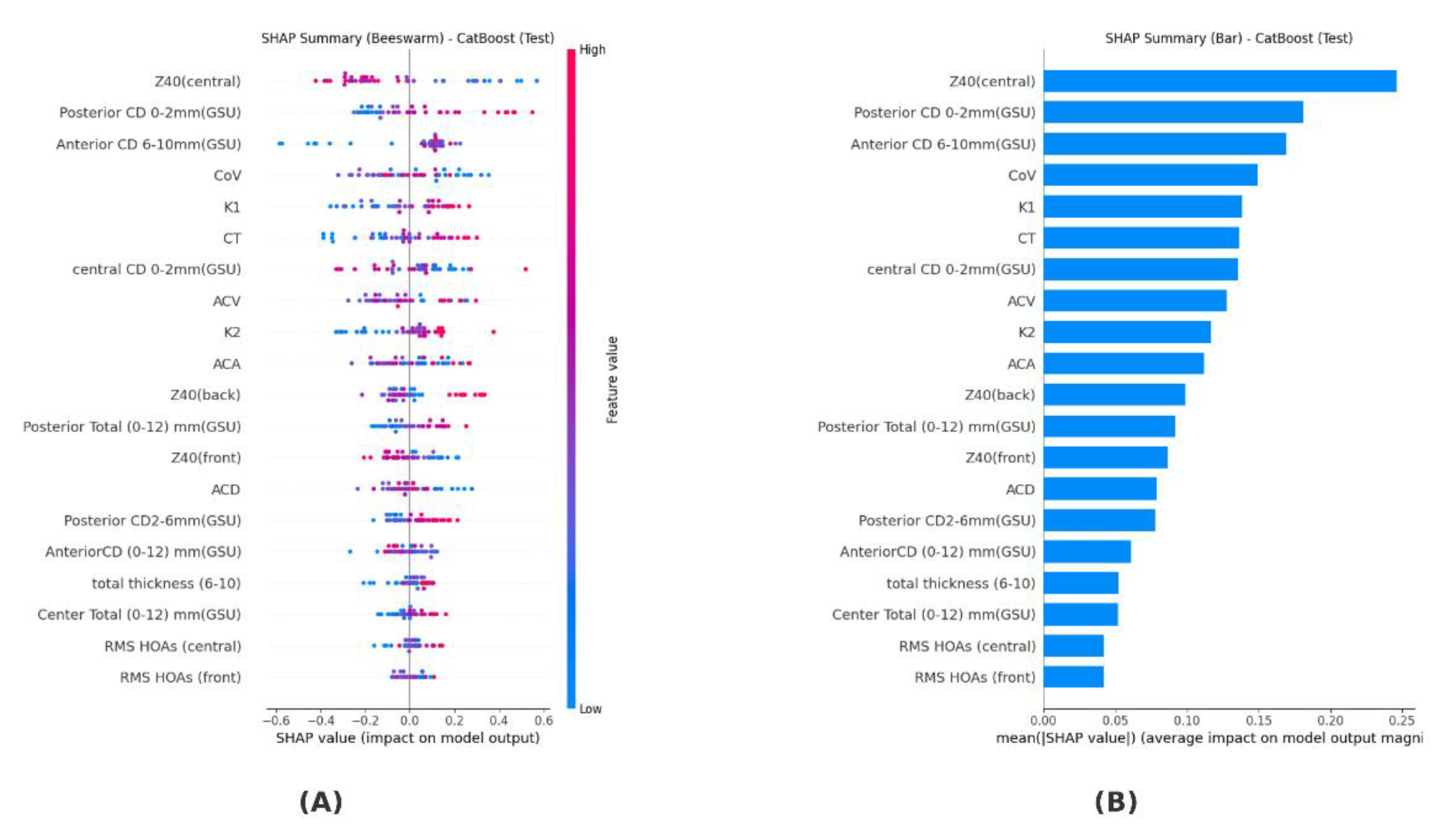
Figure 2.
Comparative ROC curves for different classification models.
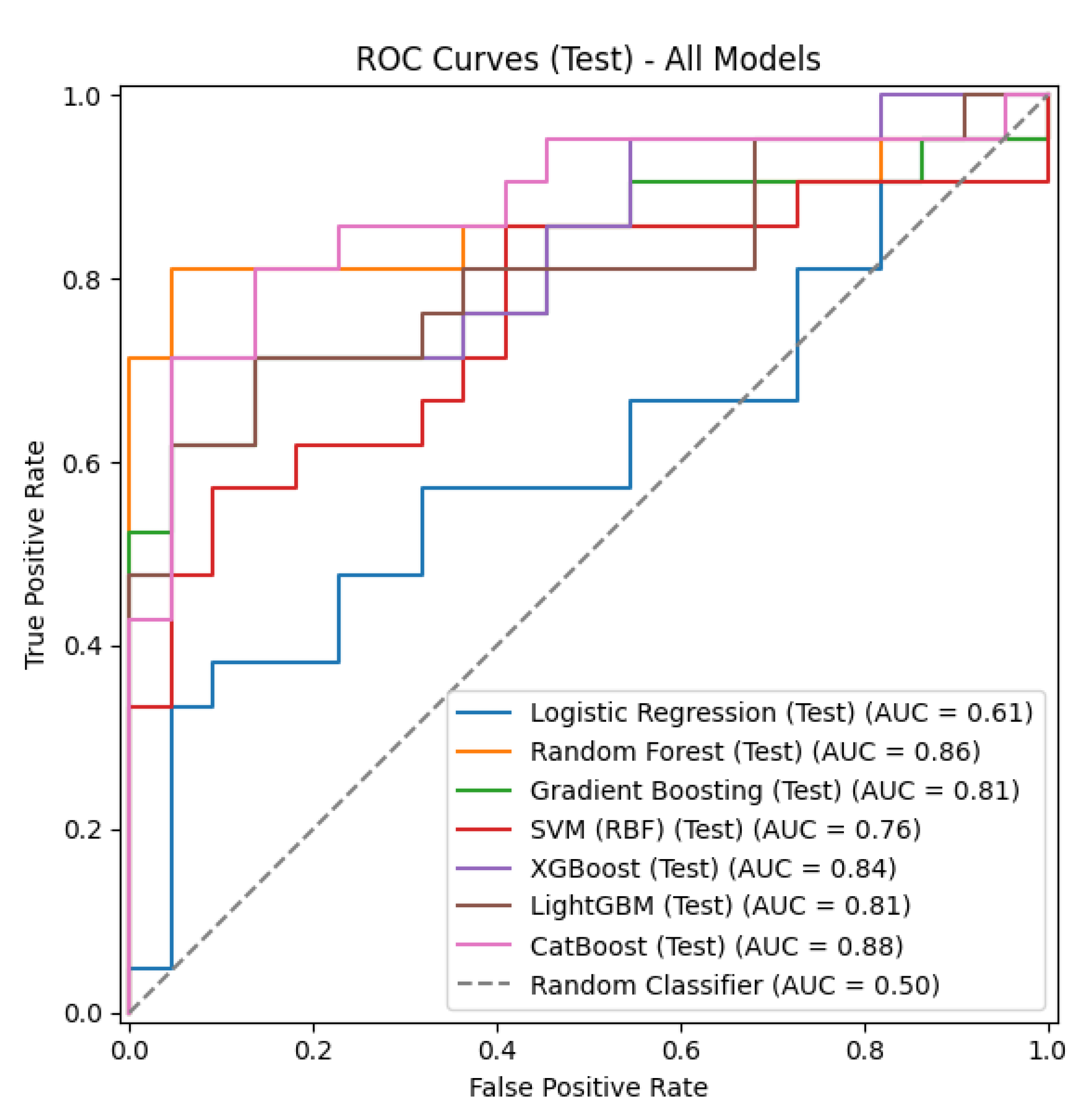
Table 1.
The input and output factors/features used in analysis.
| Variable Name | Explanation | Type | Role |
|---|---|---|---|
| Group | Study group (1 = control; 2 = psoriasis patient) | categorical | output |
| Anterior CD 0–2 mm (GSU) Anterior CD 2–6 mm (GSU) Anterior CD 6–10 mm (GSU) Anterior CD 10–12 mm (GSU) |
Densitometer measurements in the anterior 120 µm layer of the cornea (different ring regions) | continuous | input |
| Anterior CD 0–12 mm (GSU) | Total average densitometer value in the anterior layer of the cornea | continuous | input |
| Central CD 0–2 mm (GSU) Central CD 2–6 mm (GSU) Central CD 6–10 mm (GSU) Central CD 10–12 mm (GSU) |
Densitometer measurements in the central layer of the cornea (different ring regions) | continuous | input |
| Center total 0–12 mm (GSU) | Total average densitometer value of the central layer | continuous | input |
| Posterior CD 0–2 mm (GSU) Posterior CD 2–6 mm (GSU) Posterior CD 6–10 mm (GSU) Posterior CD 10–12 mm (GSU) |
Densitometer measurements in the posterior 60 µm layer of the cornea (different ring regions) | continuous | input |
| Posterior total 0–12 mm (GSU) | Total average densitometer value of the posterior layer | continuous | input |
| Total thickness (0–2) | Densitometer measurements for the entire thickness of the cornea (different ring regions) | continuous | input |
| Total thickness (2–6) | continuous | input | |
| Total thickness (6–10) | continuous | input | |
| Total thickness (10–12) | continuous | input | |
| Total thickness (0–12) | Total average densitometer value for all thicknesses | continuous | input |
| CoV | Corneal volume (mm3) | continuous | input |
| ACV | Anterior chamber volume (mm3) | continuous | input |
| ACA | Front chamber angle (degrees) | continuous | input |
| ACD | Anterior chamber depth (mm) | continuous | input |
| CT | Thinnest corneal thickness (µm) | continuous | input |
| K1 | Plain keratometry (diopter) | continuous | input |
| K2 | Vertical keratometry (diopter) | continuous | input |
| Kmax | Maximum keratometry (diopter) | continuous | input |
| RMS LOAs (front) RMS LOAs (back) RMS LOAs (central) |
Root mean square (RMS) value of low-order aberrations value (front/rear surface) |
continuous | input |
| RMS HOAs (front) RMS HOAs (back) RMS HOAs (central) |
RMS value of high-order aberrations (front/back surface) | continuous | input |
| RMS Total (front) RMS Total (back) RMS Total (central) |
RMS value of total aberrations (front/back surface/central) | continuous | input |
| Z40 (front) Z40 (back) Z40 (central) |
Corneal aberration (front/back surface/central) | continuous | input |
Table 2.
Confusion matrix.
| Predictive Condition | Actual Condition | |
|---|---|---|
| Negative | Positive | |
| Negative | True Negative (TN) | False Negative (FN) |
| Positive | False Positive (FP) | True Positive (TP) |
Disclaimer/Publisher’s Note: The statements, opinions and data contained in all publications are solely those of the individual author(s) and contributor(s) and not of MDPI and/or the editor(s). MDPI and/or the editor(s) disclaim responsibility for any injury to people or property resulting from any ideas, methods, instructions or products referred to in the content. |
© 2025 by the authors. Licensee MDPI, Basel, Switzerland. This article is an open access article distributed under the terms and conditions of the Creative Commons Attribution (CC BY) license (http://creativecommons.org/licenses/by/4.0/).
Copyright: This open access article is published under a Creative Commons CC BY 4.0 license, which permit the free download, distribution, and reuse, provided that the author and preprint are cited in any reuse.


