Submitted:
03 October 2025
Posted:
08 October 2025
You are already at the latest version
Abstract
The efficient locomotion of autonomous driving and robotics suggests a clearer visual-ization and a more precise map. This paper presents a high accuracy online mapping with weight matching LiDAR-IMU-GNSS odometry and object-level highly dynamic point cloud filtering method based on pseudo-occupancy grid. The odometry integrates IMU pre-integration, ground points through progressive morphological filtering(PMF), motion compensation and weight feature point matching. Weight feature point matching enhances alignment accuracy by combining geometric and reflectance inten-sity similarities. By justifying the pseudo-occupancy ratio between the current frame and prior local submaps, grid probability value is updated to identify the distribution of dynamic grids. Object-level point cloud clusters segmentation is obtained using curved voxel clustering method, eventually leading to filtering out the object-level highly dy-namic point clouds during the online mapping process. The proposed odometry, in comparison with LIO-SAM and FAST-LIO2 frameworks, shows superior accuracy in the KITTI, UrbanLoco, and Newer College (NCD) datasets. Meantime, the proposed highly dynamic point cloud filtering algorithm also shows a better detection precision than the performance of Removert and ERASOR. Furthermore, the high accuracy online map-ping is built from a real-time dataset with the comprehensive filtering of driving vehi-cles, cyclists and pedestrians. This research contributes to field of the high accuracy online mapping, especially in filtering the highly dynamic objects in an advancing way.
Keywords:
odometry
; weight matching
; object-level highly dynamic point cloud
; pseudo-occupancy grid
1. Introduction
LiDAR mapping technology has achieved remarkable progress and been widely applied in various fields, including autonomous driving[1,2,3], SLAM system[4,5,6] and robotic navigation[7,8,9,10]. Particularly in robotics[9,10,11], the synergistic integration of multi-sensors and computer vision has revolutionized the environmental perception capabilities of intelligent agents.
Recent research shows that information fusion obtained from a Global Navigation Satellite System(GNSS), an Inertial Measurement Unit(IMU) and a LiDAR sensor has achieved high-precision mapping and localization in complex environments[12,13]. But in reality, the presence of dynamic objects poses significant challenges to precision in LiDAR mapping. On one hand, conventional point cloud matching algorithms generally assume a static environment. This assumption holds in most cases due to short single-frame scanning time, and thus the impact of dynamic objects on odometry accuracy can be negliable[14]. But when objects move in a high speed, the resulting point cloud distortion severely disrupts matching precision, leading to accumulated localization errors. In some cases, moving objects introduced as "ghost artifacts"[15,16] appeared into the generated map. The resulting map redundancy consequently misleads localization and path planning terribly, decreasing accuracy and safety in navigation decision-making. Therefore, to effectively suppress and eliminate the side effects of highly dynamic point clouds on map is of great significant in enhancing the reliability and practicality of LiDAR mapping systems.
According to real-time performance of disposing sensor data in dynamic environments, dynamic point cloud filtering algorithms can generally be categorized into two classes: online filtering and post-processing-based filtering. Online filtering methods usually select several consecutive point cloud frames as a reference, and then compared them with the target frame in order to achieve superior real-time performance. For instance, RF-LIO[17], an extension of LIO-SAM[18], leverages the information from initial pose of frontend odometry and local submaps to filter dynamic points on the current frame adaptively and iteratively, eventually generating a static global map. ETH-Zurich’s ASL Lab proposed an end-to-end dynamic object detection framework[19], which is based on occupancy grids. This framework automatically labels dynamic objects and then trains them in the 3D-MiniNet, which enables online detection and filtering of dynamic point clouds. Post-processing methods utilize all frames during the entire SLAM cycle as reference, thus achieving a higher accuracy and precision. Peopleremover algorithm[20] constructs a regular voxel occupancy grid and then determine free voxels by traversing the lines of sight from the sensor to the measured points through the voxel grid. ERASOR[21], proposed by Hyungtae Lim et al., detects dynamic points by comparing region-wise occupancy ratios between the current scan and local submaps. The ratios exceeding a threshold are marked as dynamic. Removert[22], presented by Giseop Kim et al., built a novel 2D depth map by projecting a 3D point cloud with its neighboring submaps. By comparing the pixel depths at the same positions on the two maps, the shallower one is considered a dynamic point. This method outperforms manual annotations on the SemanticKITTI dataset[23], demonstrating an excellent filtering efficacy.
In real-world scenarios, to ensure accurate decision-making at high speeds, the real-time performance of maps must be guaranteed as a priority. However, at the same time, to optimize the effectiveness of decision-making and the robustness of motion behaviors, the map is required to be built in a sufficiently high accuracy. In order to address it, therefore, this paper improves the precision of LiDAR-IMU-GNSS multi-sensor mapping by analyzing the geometric and reflective similarities of point cloud matching points to determine weight coefficients, and then employs a pseudo-occupancy grid-based method to filter object-level highly dynamic point clouds in real time, ultimately effectively enhancing the accuracy and efficiency in mapping. Simulation experiments demonstrate that the accuracy of this odometry system surpasses that of LIO-SAM and FAST-LIO2 based on KITTI, UrbanLoco[24], and Newer College[25] (NCD) datasets. Compared to the Removert and ERASOR algorithms, the filtering of highly dynamic point clouds in this paper is more effective. The proposed algorithm is applied in a real-time dataset to build the map online with successful filtering of driving vehicles, cyclists and pedestrians.
2. Algorithm Framework
This paper proposes an online mapping algorithm of high accuracy multi-sensor fusion of LiDAR-IMU-GNSS and object-level highly dynamic point filtering. The framework consists of data preprocessing, weight feature point matching, and dynamic point filtering, as shown in Figure 1.
i) Data preprocessing: Raw point cloud data from LiDAR, IMU, and GNSS are processed to generate synchronized and fused multi-sensor measurements, including IMU pre-integration, ground points through PMF and motion compensation.
ii) Weight feature point matching: the weight coefficient of Mahalanobis distance is determined by geometric and reflectance intensity similarities to obtain the optimized pose.
iii) Dynamic point filtering: dynamic objects is removed from the point cloud and map is built in real time by means of a pseudo-occupancy grid filtering algorithm.
3. Data Fusion for Weight Matching LiDAR-IMU-GNSS Odometry
3.1. IMU Pre-Integration
IMU pre-integration constructs constraints between LiDAR keyframes to suppress odometry drift and establish a pose graph, including attitude, velocity and position information. After acquirement of IMU data and consideration for bias and noise, the predicted values of pre-integration for attitude , velocity and position between frame and is derived by discrete-time integration method. Thus, yielding their relative differences , and in Equation (1),
where and represent the angular velocity measured by the gyroscope and linear acceleration by accelerometer at kth frame, respectively. and denote the bias noise of the angular velocity and acceleration at kth frame. and are the measurement biases of the angular velocity and acceleration at kth frame. is the time interval between kth frame and (k+1)th frame in the IMU data. represents gravity. denotes the mapping from a rotation vector to a rotation matrix. Therefore, the state at (k+1)th frame can be predicted by integrating the state at kth frame.
Assuming that the IMU biases and within a short period, the noise terms can be simplified further. According to the linear approximation in Lie group theory, we establish the relationship between the predicted , and and the measured , and . And the measured values are written as follows.
On the left-hand side of Equation (2) are the predicted values derived from the state variables, and the right-hand side are the measured values obtained through IMU integration and a random noise term. In order to explicitly represent the measured values in Equation (2), it is necessary to obtain the state transition equations for random noise terms.
Equation (3) reveals that differs from by a noise term . By applying operator which denotes the mapping from a rotation matrix to a rotation vector, the noise term can be simplified linearly. The first-order term is kept and the is expressed as,
where is the Jacobian matrix. represents (j-1)th the bias noise of the angular velocity. is transpose.
Assuming that noise terms of , and as well as the bias noise of the IMU all satisfy zero-mean Gaussian distributions, we derive the following expression,
Similar procedures are applied in and terms. The state transition equation of is given by,
where denotes the identity matrix. Consequently, the state transition equation for covariance matrix of noise term is derived as,
IMU biases varying with time severely influences the accuracy of measurement. By assuming that pre-integrated measurements vary with IMU biases linearly, we retain the first-order partial derivatives of pre-integrated measurements relative to the biases, so as to compensate for bias-induced errors in pre-integration.
3.2. Ground Point Segmentation
The point cloud of the keyframe is extracted for reducing storage. In order to achieve the adaptive adjustment of the keyframe threshold, parameter is determined according to the surrounding. Therefore, the keyframe threshold is expressed in Equation (8).
where , is the median of the Euclidean distances from the point cloud of the current frame to the origin of the LiDAR. represents the openness of the scanning environment in the previous frame. and are constant, and , .
During online mapping, the Progressive Morphological Filtering (PMF) algorithm is used to segment ground points and non-ground points in each keyframe point cloud in real time.
PMF optimizes window dimension by gradually increasing the window size of the filtering. The update principles of the filtering window size and the height difference threshold are shown in Equation (9).
where denotes the window size at the kth iteration. represents the initial window size. and refer to the initial and maximum height difference threshold. indicates the slope, and . stands for the grid size.
3.3. Motion Compensation of LiDAR Point Clouds
At high vehicle speed, motion distortion compensation for point clouds becomes essential. If IMU data is available, the IMU-based motion compensation in continuous time is used. Otherwise, in the case of IMU data dropout, the motion compensation method based on the constant velocity model is adopted. Assuming that the current frame keeps the same motion state as the previous frame of the LiDAR, the LiDAR pose at each timestamp within the current frame can be calculated by interpolation.
where and denote the query point's attitude and position. represents the current timestamp.
3.4. Weight Feature Point Matching Method based on Geometric-Reflectance Intensity Similarity
Mahalanobis distance between points is generally use as the criterion for feature point matching, and further in order to obtain the optimized pose. However, this method with the same weight assigned to each matched point fails to accurately represent the influence from the uncertainty of different matched point pairs. During the process of point matching, the weight of false matches should be significantly reduced. Besides, the position uncertainty of the two matched points produces noise, and thus the weight of such points should decrease as their uncertainty increases.
For the sake of both improving point matching accuracy and promoting calculation efficiency, an eigenvalue-based approach is employed for extracting planar feature points. Thus, the centroid and the covariance matrix of the point distribution around point is given in Equation (11) based on the KD-Tree method.
where , and are the three eigenvalues of the covariance matrix.
If eigenvalues satisfy Equation (12), point is a planar feature point.
where and are thresholds.
In order to reduce incorrect matching, the similarity between the two feature points should be taken into account. By assigning different weights to each point, the residual function for point cloud matching can be formulated. In this section, a weight feature point matching method based on the geometric-reflectance intensity similarity of point clouds is proposed.
The geometric similarity is defined by the positional relationship between the normal vectors of the planar feature points in one point cloud and in the target point cloud, separately. Note that is the smallest eigenvalue, its eigenvector is thus approximately equivalent to the normal vector of the corresponding plane. The subscript and correspond to points and points . Therefore, the geometric similarity can be expressed as,
The reflection intensity of matched points exhibits similar distributions, thus chosen as the second similarity. Assuming that the reflection intensity around points and follows normal distributions and , respectively, and the distances from two points to the sensor center are and , with (where is the scale factor), their reflection intensity satisfies scaling law as well. Therefore, a modified Kullback-Leibler (KL) divergence model is yield based on Lambertian theory,
Since the weight coefficient is not larger than 1, a Gaussian function is used to normalize the Kullback-Leibler (KL) divergence, and thus the reflection intensity similarity is obtained in Equation (15).
where is Gaussian scale factor.
To avoid the sparsity error, the average planarity of points and is introduced as the third weight coefficient.
Eventually, the weight of points and is defined as,
To ensure the real-time performance of the odometer, the planar feature point cloud of the current frame is matched with that of the local submap in the keyframe. The transform matrix is obtained by minimizing the weighted Mahalanobis distance obtained from the local geometric characteristics, as shown in Equation (18).
where represents the Mahalanobis distance constructed by the GICP algorithm. represents the transformation error term between the current frame and the local submap of the keyframe. represents the covariance matrix of the points. The superscript and represents the covariance matrix of the current frame and the submap, respectively. For the covariance matrix , since all the feature points are planar points, the diagonal elements of are replaced with (1,1,ϵ), where ϵ is a very small constant, to regularize the covariance matrix .
4. Online Filtering Method for Highly Dynamic Point Clouds
If the set of keyframe point clouds is , after extracting the ground points, they are divided into ground points and non-ground points . Furthermore, the point cloud set obtained by transforming each keyframe point cloud into the global coordinate system and then splicing them together is the map . If the highly dynamic point cloud map is, then the static point cloud map can be expressed as . Removing point cloud in a map probably leads to point cloud loss and over-filtering, but removing only the point clouds of one frame or several frames, the point clouds of other frames can still fill the loss in the map. Thus, we obtain the static map by filtering the object-level highly dynamic point clouds at each keyframe, shown in Equation (19).
where is the ground point cloud of the kth keyframe, which is regarded as static point cloud. represents object-level highly dynamic point cloud set of the kth keyframe. denotes all object-level point clouds in the kth keyframe.
Objects that generate highly dynamic points, such as pedestrians, vehicles, and so forth, temporarily occupy a certain area in the map within a short time, while static points persistently remain in fixed areas. Therefore, by comparing the grid occupancy between the current frame’s point cloud and the map, we can identify regions occupied by dynamic objects. Consequently, non-ground points within these dynamic regions can be classified as highly dynamic points.
First, to eliminate the influence of abnormal points in the point cloud, a pass-through filter is applied to extract the region of interest. The filtering range is set from to . Then, the point cloud of the region of interest in the current keyframe is represented as,
The grid obtained from the point cloud of the region of interest in the global coordinate system is . Thus the local submap can be represented in the Equation (21).
where the grid projection function is defined as , and are the grid resolutions in the X and Y dimensions, respectively. is the index of the grid corresponding to the point .
The pseudo-occupancy rate is defined as the difference between the maximum and minimum heights of the point cloud within the grid. And thus, the rates and of the current keyframe and the local sub-map are expressed as follows,
where represents the grid with index , and represent the minimum values of the point cloud heights of the grid with index in the local submap and the current keyframe respectively.
The pseudo-occupancy ratio determines the occupancy status of dynamic point clouds in the current frame's grid, and is defined to the ratio between the current frame and the submap grid in Equation (23).
where is the threshold for the pseudo-occupancy ratio. If the pseudo-occupancy ratio exceeds , the grid in the current frame is considered to contain dynamic point clouds.
The joint distribution of the binary states for pseudo-occupancy grids is expressed as follows,
where represents the occupancy state of the ith grid, and denotes all observations up to frame , where each observation corresponds to the difference between the scan at frame and the map.
Update the probability information in the map grid according to Bayes' rule, that is,
where defines the occupancy and non-occupancy of the grid, and .
The update rule for is as follows,
where are increased by a gain factor () for , and thus the updated probability value . For and , the grid is still likely occupied by dynamic points, and updated using . Otherwise, retain its initial value . represents an initial prior probability.
In order to avoid deleting objects with ambiguous boundary by mistake, a curved voxel point cloud clustering algorithm is adopted[26]. This algorithm helps detect the point cloud corresponding to the object in the map, and then the object-level segmentation of the highly dynamic point cloud in the map is further carried out. If all objects containing dynamic grids are filtered out without distinguishing the dynamic attributes of the objects, static objects may be deleted by mistake. Therefore, the object dynamic score for each object point cloud is defined in Equation (27) as the dynamic evaluation criterion to separate the highly dynamic object point cloud completely.
where represents the number of point clouds of the ith object. represents the grid corresponding to each point in the object , and the function returns the corresponding value according to the probability value of the grid. The definition is as follows,
where the true probability of the grid is returned when the grid probability is greater than the initial value . Otherwise, a constant () is returned. It should be noted that when the grid is always occupied by a static object, the probability of the grid is always , and the log odds value of the grid is always . When both static and dynamic objects exist in the grid, due to the existence of , the object dynamic score is reduced, and the probability of mistakenly deleting the static object is also reduced. The finally obtained dynamic object point cloud is,
where is the inverse of the log odds function, converting the log odds back to a probability value, and is the adaptive probability threshold for dynamic objects. is the point cloud cluster.
When performing point cloud clustering, it is possible that two objects close to each other are identified as a single point cloud cluster. As a result, static objects within may be removed incorrectly. Since such point clouds typically occupy a large number of grids but a small proportion of highly dynamic grids, they can be distinguished based on the total number of occupied grids and the proportion of dynamic grids, as shown in Equation (30).
The weights of point cloud features have been taken into account by LiDAR-IMU-GNSS odometry when computing the Mahalanobis distance of the matching point cloud.
where represents the number of grids occupied by the point cloud cluster . represents the minimum threshold of occupied grids. represents the number of dynamic grids in the point cloud cluster . represents the maximum proportion threshold of dynamic grids.
After deleting highly dynamic grids in the under-segmented point cloud, the static map is eventually established.
5. Algorithm Validation
5.1. Accuracy of Proposed Odometry Systems
For the sake of accuracy validation of the proposed weight matching LiDAR-IMU-GNSS odometry, our method is tested in the KITTI, UrbanLoco[24], and Newer College[25] (NCD) datasets in comparison with LIO-SAM and FAST-LIO2 methods.
Figure 2 presents the trajectory comparison between the proposed algorithm and the LIO-SAM algorithm on 00 sequences of the KITTI dataset. The ground truth, LIO-SAM trajectory and the trajectory of the proposed algorithm are shown in green, blue and red colors, separately. Obviously, the trajectory of the proposed algorithm is significantly closer to the ground truth, indicating that its accuracy is higher than that of the LIO-SAM algorithm.
The Root-Mean-Squared Error (RMSE) of the Absolute Trajectory Error (ATE) was used to evaluate the error across the entire trajectory. The RMSE is defined as follows:
where represents the number of frames in the dataset. denotes extracting the translational component of the pose, and the Euclidean norm is used for vector magnitude computation in the RMSE calculation.
Table 1 summarizes the RMSE for the three algorithms across subsets of the KITTI, UrbanLoco, and NCD datasets. The results indicate that the proposed algorithm achieves higher accuracy than the other two open-source algorithms in most datasets, thus demonstrating superior performance.
5.2. Comparison of Highly Dynamic Point Cloud Filtering Algorithm
Figure 3 and 4 gives the visualization result of the proposed highly dynamic point cloud filtering algorithm, the Removert and ERASOR algorithms based on the sequence 00 and 05 of the SemanticKITTI dataset. In the figures, the red point clouds represent the highly dynamic object point clouds detected by the corresponding algorithm, while the blue ones represent the static point clouds.
In Figure 3(a) and 3(b), compared with the ground truth, it can be seen that the Removert algorithm and ERASOR algorithm can basically filter out dynamic points, but they incorrectly remove a large number of static points. Finally, excessive false positives points in detection lead to a relatively sparse map generated. In contrast, the proposed method in this paper ensures a high detection precision while having fewer false positive points. In Figure 4, based on sequence 05 dataset, the Removert algorithm achieves a relatively low detection precision, and the ERASOR algorithm has a relatively high proportion of false positives, while the algorithm proposed in this paper outperforms the above two algorithms on this dataset.
Furthermore, based on the sequences 00, 01, 05, and 07 of the SemanticKITTI datasets, which contain many dynamic objects, the accuracy of the proposed highly dynamic point cloud filtering algorithm is compared with Removert and ERASOR algorithms. Table 2 presents the Preservation Rate (PR), Recall Rate (RR), and F1 score of the proposed highly dynamic point cloud filtering module compared with Removert and ERASOR algorithms. The three metrics are defined as follows:
where TP (True Positive) represents the number of samples that are correctly detected as dynamic object categories. FP (False Positive) represents the number of samples that are actually static but detected as dynamic categories. FN (False Negative) represents the number of samples that are actually dynamic but detected as static categories. The values of all three metrics range from 0 to 1, and the closer they are to 1, the better the performance.
Table 2 presents the performance of Removert, ERASOR, and the proposed method in this paper across three metrics on the SemanticKITTI dataset. It can be observed that the proposed highly dynamic point cloud filtering algorithm in this paper exhibits high accuracy, with fewer missed detections and false detections. It can effectively filter high dynamic objects in single-frame scanned point clouds and eliminate the "long trailing shadows" in the map caused by moving objects.
5.3. Online Filtering Experiment
A dataset at an intersection on the campus of Beijing Institute of Technology (BIT) is obtained in order to test the proposed online highly dynamic point cloud filtering algorithm in this paper. The intersection contains numerous highly dynamic objects, such as heavy traffic and a large pedestrian flow.
In the experiment, the Wuling Hongguang miniEV serves as the test vehicle, which equips with an environmental perception system including three sensors. The Robosense Helio-32 mechanical LiDAR offers a 360° horizontal field of view and 70° vertical field of view, with the ranging accuracy within 2cm and the 10Hz scanning frequency. The GW-NAV100B is a dual-antenna high-precision MEMS integrated navigation. It incorporates a built-in three-axis gyroscope, a three-axis accelerometer, and a four-mode (BD/GPS/GLONASS/GALILEO) receiver, enabling it to measure the velocity, position and attitude of the test car. Xsens Mti-630 is a 9-axis IMU with a 100Hz output frequency. During the data collection process, the total duration in this experiment was approximately 1000s, covering a distance of about 3000m. Meantime, to construct local sub-maps, the data was equally divided into five segments, with each is approximately 600m long.
Two typical highly dynamic scenarios are shown in Figure 5 and 6. The black point clouds represent static environmental point clouds, while the red point clouds represent the highly dynamic objects detected by the proposed method in this paper.
In Figure 5 and 6, it can be observed that at the intersection, there are a large number of point cloud "long trailing shadows" caused by pedestrians, cyclists, and vehicles, which degrades the quality of the point cloud map. Typical highly dynamic objects, such as driving vehicles, cyclists and pedestrians, can be picked up. In Figure 5, the blue and green boxes respectively enclose the detailed point cloud maps of vehicles and cyclists; in Figure 6, the blue and green boxes respectively enclose the detailed point cloud maps of vehicles and pedestrians. As can be seen from Figure 5 and 6, the online highly dynamic point cloud filtering algorithm proposed in this paper can effectively detect major highly dynamic objects such as pedestrians, cyclists, and vehicles in highly dynamic scenarios.
6. Conclusions
This paper improves the mapping method with weight matching LiDAR-IMU-GNSS odometry and a proposed online highly dynamic point cloud filtering algorithm. The weight matching LiDAR-IMU-GNSS odometry includes IMU pre-integration, ground points extraction, motion compensation and weight feature point matching. Specifically, within the weight matching LiDAR-IMU-GNSS odometer, a method for point cloud keyframe selection and sub-map construction based on an adaptive threshold is designed. Ground point clouds and plane point clouds are extracted respectively using PMF and KD-Tree methods. A weight feature point matching method based on geometric-reflectance intensity similarity is proposed, which improves the accuracy of point cloud matching. Subsequently, taking the pseudo-occupancy ratio between the current frame point cloud and the previous local sub-map as an observation, the probability values of the grid are updated to obtain the distribution of dynamic feature in the map. In addition, the curved voxel point cloud clustering algorithm is used to obtain object-level point cloud clusters. Thereby, this algorithm realizes complete filtering of highly dynamic object-level point clouds.
The higher accuracy of the weight matching LiDAR-IMU-GNSS odometer is valid in the KITTI, UrbanLoco, and NCD datasets in comparison with LIO-SAM and FAST-LIO2 methods. The proposed highly dynamic point cloud filtering algorithm outperforms the Removert and ERASOR algorithms based on the sequences of the SemanticKITTI dataset. Finally, online mapping with highly dynamic point cloud filtering is applied in a real-time dataset, and typical highly dynamic objects, such as driving vehicles, cyclists and pedestrians, can be clearly picked up. We hope that this research can benefit the research about high accuracy mapping online with the filtering of highly dynamic objects, and promote the development of navigation and locomotion of in autonomous driving and robotics.
Author Contributions
Zhao Xin: conceptualization, methodology, writing—original draft and funding acquisition. Cao Xingyu: methodology, resources and writing—review and editing; Ding Meng: investigation and formal analysis. Jiang Da: writing—review and editing; Wei Chao: conceptualization, supervision and project administration. All authors have read and agreed to the published version of the manuscript.
Funding
This work was supported by the State Administration of Science. Technology and Industry for National Defense Project(No. 8KD006(2024)-2).
Data Availability Statement
The data that support the findings of this study are available from the corresponding author upon reasonable request.
Conflicts of Interest
The authors declare no conflicts of interest.
References
- Faisal, A.; Kamruzzaman, M.; Yigitcanlar, T.; et al. Understanding autonomous vehicles[J]. Journal of transport and land use 2019, 12, 45–72. [Google Scholar]
- Cao, X.; Wei, C.; Hu, J.; et al. RDP-LOAM: Remove-Dynamic-Points LiDAR Odometry and Mapping[C]//2023 IEEE International Conference on Unmanned Systems (ICUS). IEEE, 2023: 211-216.
- Xu, H.; Chen, J.; Meng, S.; et al. A Survey on Occupancy Perception for Autonomous Driving: The Information Fusion Perspective[J]. 2024.
- Hu, J.; Mao, M.; Bao, H.; et al. CP-SLAM: Collaborative Neural Point-based SLAM System[J]. 2023.
- Pan, Y.; Zhong, X.; Wiesmann, L.; et al. PIN-SLAM: LiDAR SLAM Using a Point-Based Implicit Neural Representation for Achieving Global Map Consistency[J].IEEE Transactions on Robotics, 2024.
- Kerbl, B.; Kopanas, G.; Leimkuehler, T.; et al. 3D Gaussian Splatting for Real-Time Radiance Field Rendering[J].ACM-Transactions on Graphics 2023, 42.
- Zhu, S.; Mou, L.; Li, D.; et al. VR-Robo: A Real-to-Sim-to-Real Framework for Visual Robot Navigation and Locomotion[J]. 2025.
- Wang, Z.; Chen, H.; Fu, M. Whole-body motion planning and tracking of a mobile robot with a gimbal RGB-D camera for outdoor 3D exploration[J].Journal of Field Robotics, 41:604[2025-09-08].
- Longo, A.; Chung, C.; Palieri, M.; et al. Pixels-to-Graph: Real-time Integration of Building Information Models and Scene Graphs for Semantic-Geometric Human-Robot Understanding[J]. 2025.
- Tourani, A.; Bavle, H.; Sanchez-Lopez, J.L.; et al. Visual SLAM: What are the Current Trends and What to Expect?[J]. 2022.
- Ye, K.; Dong, S.; Fan, Q.; et al. Multi-Robot Active Mapping via Neural Bipartite Graph Matching[J]. 2022.
- Hester, G.; Smith, C.; Day, P.; et al. The next generation of unmanned ground vehicles[J]. Measurement and Control 2012, 45, 117–121. [Google Scholar] [CrossRef]
- Chen, L.; Wang, S.; McDonald-Maier, K.; et al. Towards autonomous localization and mapping of AUVs: a survey[J]. International Journal of Intelligent Unmanned Systems 2013, 1, 97–120. [Google Scholar] [CrossRef]
- Hu, X.; Yan, L.; Xie, H.; et al. A novel lidar inertial odometry with moving object detection for dynamic scenes[C]//2022 IEEE International Conference on Unmanned Systems (ICUS). IEEE, 2022: 356-361.
- Lu, Z.; Hu, Z.; Uchimura, K. SLAM estimation in dynamic outdoor environments: A review[C]//Intelligent Robotics and Applications: Second International Conference, ICIRA 2009, Singapore, December 16-18, 2009. Proceedings 2. Springer Berlin Heidelberg, 2009: 255-267.
- Liu, W.; Sun, W.; Liu, Y. Dloam: Real-time and robust lidar slam system based on cnn in dynamic urban environments[J]. IEEE Open Journal of Intelligent Transportation Systems, 2021.
- Qian, C.; Xiang, Z.; Wu, Z.; et al. Rf-lio: Removal-first tightly-coupled lidar inertial odometry in high dynamic environments[J]. arXiv:2206.09463, 2022.
- Shan, T.; Englot, B.; Meyers, D.; et al. Lio-sam: Tightly-coupled lidar inertial odometry via smoothing and mapping[C]//2020 IEEE/RSJ international conference on intelligent robots and systems (IROS). IEEE, 2020: 5135-5142.
- Pfreundschuh, P.; Hendrikx, H.F.C.; Reijgwart, V.; et al. Dynamic object aware lidar slam based on automatic generation of training data[C]//2021 IEEE International Conference on Robotics and Automation (ICRA). IEEE, 2021: 11641-11647.
- Schauer, J.; Nüchter, A. The peopleremover—removing dynamic objects from 3-d point cloud data by traversing a voxel occupancy grid[J]. IEEE robotics and automation letters 2018, 3, 1679–1686. [Google Scholar] [CrossRef]
- Lim, H.; Hwang, S.; Myung, H. ERASOR: Egocentric ratio of pseudo occupancy-based dynamic object removal for static 3D point cloud map building[J]. IEEE Robotics and Automation Letters 2021, 6, 2272–2279. [Google Scholar] [CrossRef]
- Kim, G.; Kim, A. Remove, then revert: Static point cloud map construction using multiresolution range images[C]//2020 IEEE/RSJ International Conference on Intelligent Robots and Systems (IROS). IEEE, 2020: 10758-10765.
- Behley, J.; Garbade, M.; Milioto, A.; et al. Semantickitti: A dataset for semantic scene understanding of lidar sequences[C]//Proceedings of the IEEE/CVF international conference on computer vision. 2019: 9297-9307.
- Wen, W.; Zhou, Y.; Zhang, G.; et al. UrbanLoco: A full sensor suite dataset for mapping and localization in urban scenes[C]//2020 IEEE international conference on robotics and automation (ICRA). IEEE, 2020: 2310-2316.
- Ramezani, M.; Wang, Y.; Camurri, M.; et al. The newer college dataset: Handheld lidar, inertial and vision with ground truth[C]//2020 IEEE/RSJ International Conference on Intelligent Robots and Systems (IROS). IEEE, 2020: 4353-4360.
- Park, S.; Wang, S.; Lim, H.; et al. Curved-voxel clustering for accurate segmentation of 3D LiDAR point clouds with real-time performance[C]//2019 IEEE/RSJ International Conference on Intelligent Robots and Systems (IROS). IEEE, 2019: 6459-6464.Author 1, A.B. (University, City, State, Country); Author 2, C. (Institute, City, State, Country). Personal communication, 2012.
Figure 1.
Algorithm framework
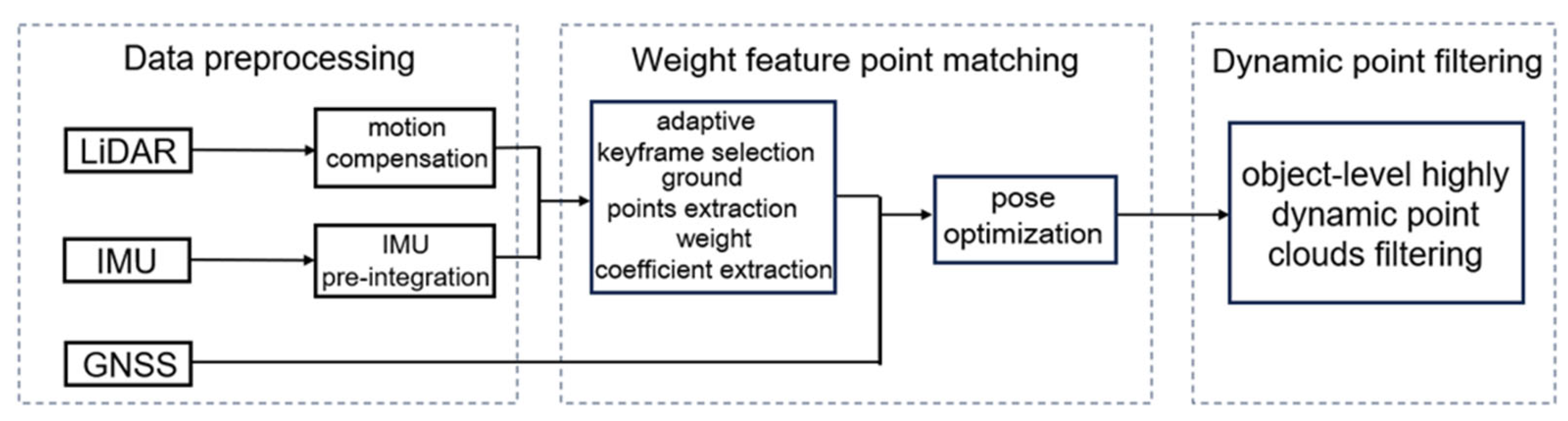
Figure 2.
00 sequence of the KITTI dataset.
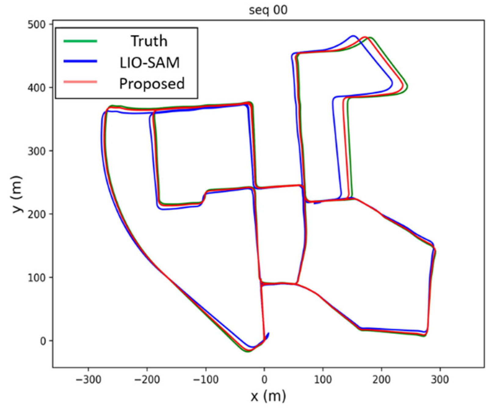
Figure 3.
Three algorithms on the sequence 00 of the SemanticKITTI dataset.
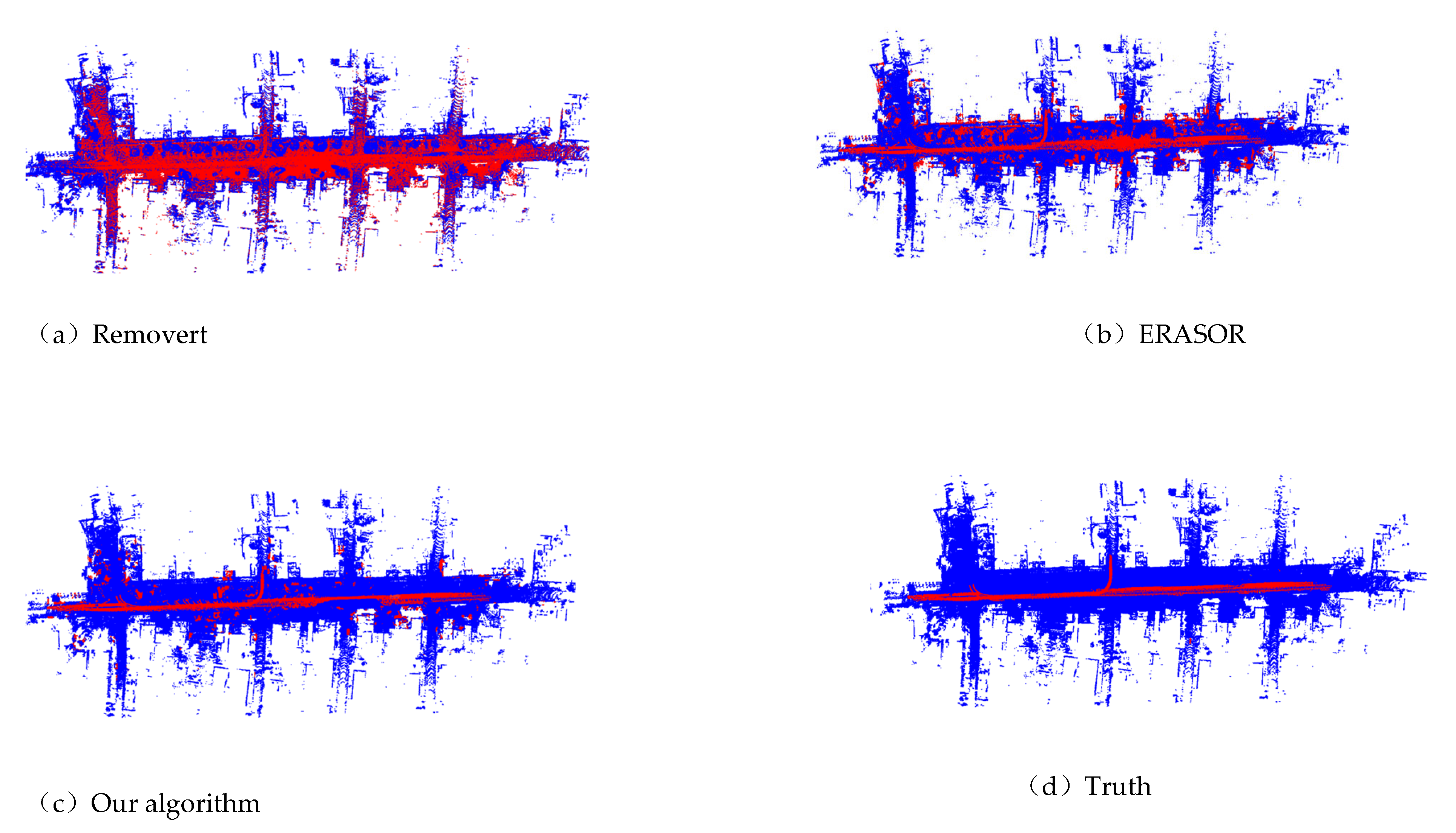
Figure 4.
Three algorithms on the sequence 05 of the SemanticKITTI dataset.
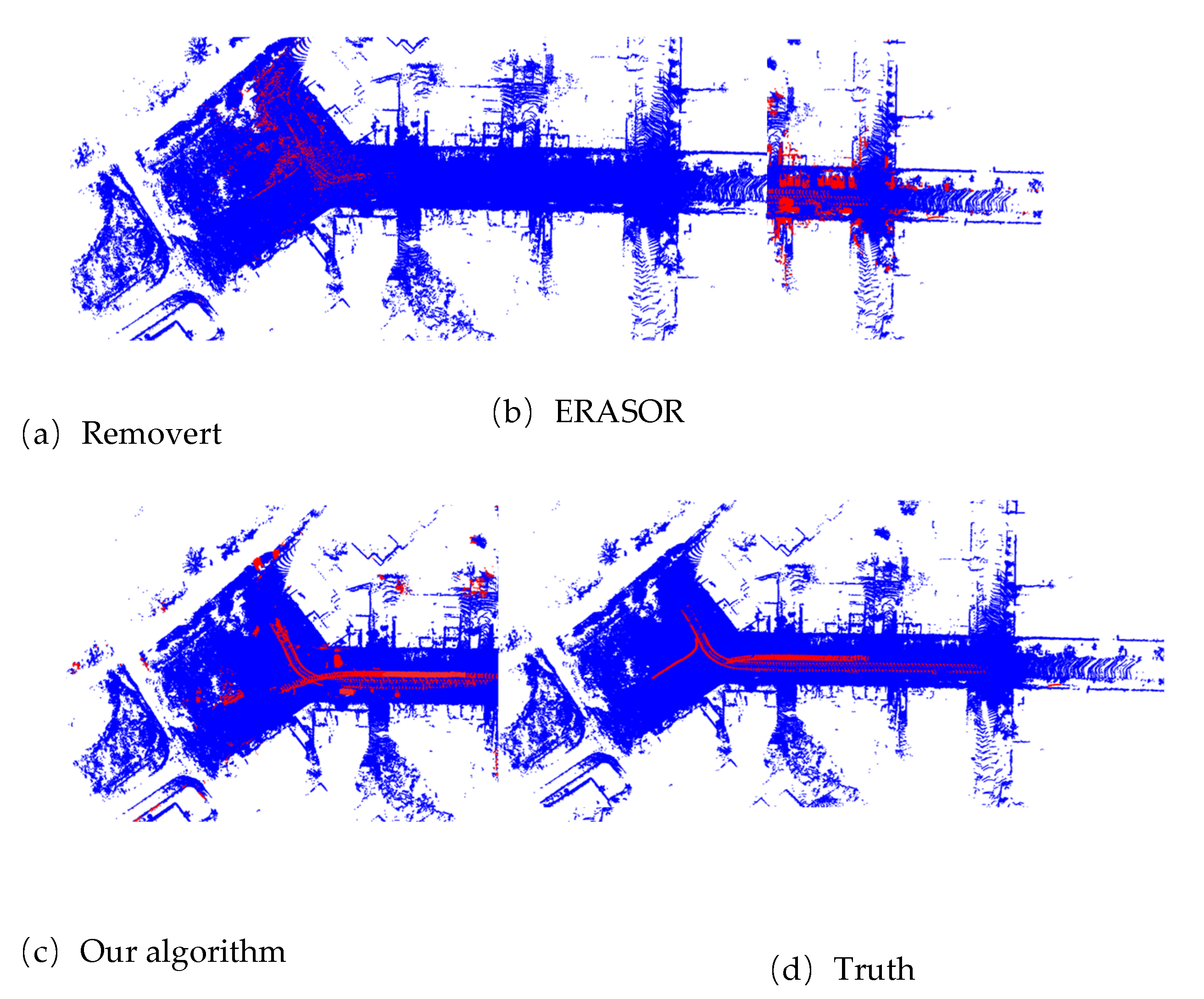
Figure 5.
Scenario 1 and highly dynamic objects.
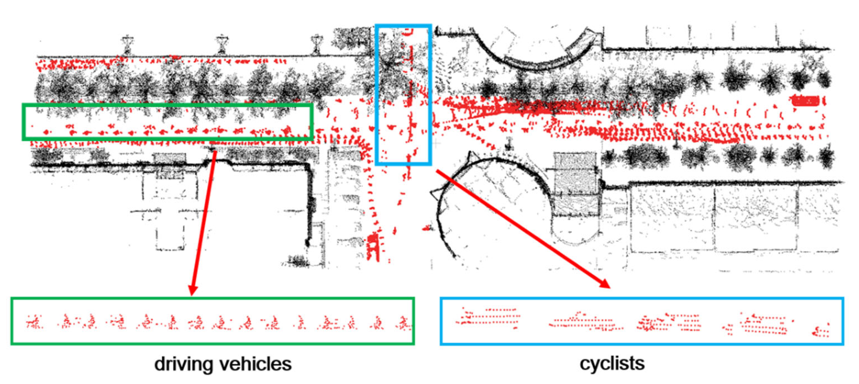
Figure 6.
Scenario 1 and highly dynamic objects.
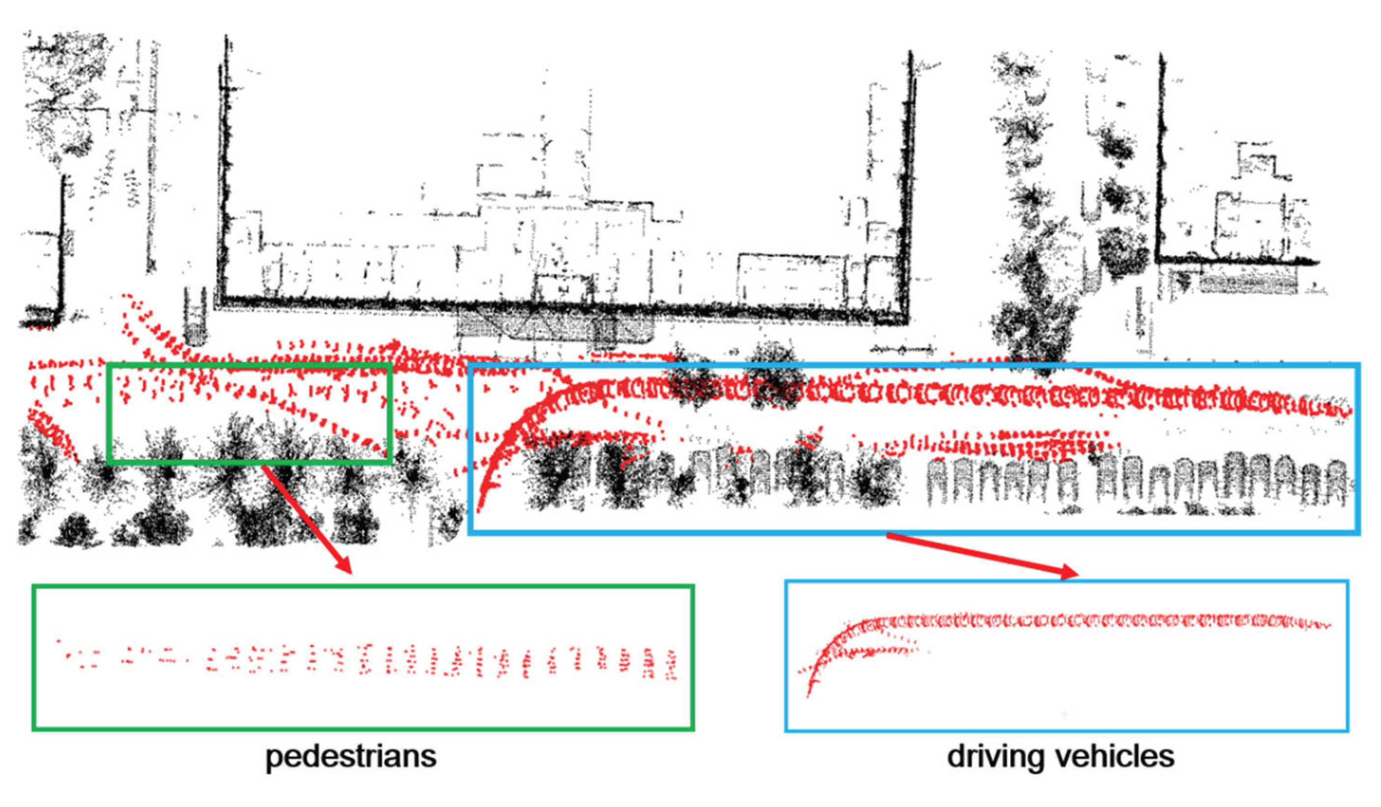

Table 1.
The RMSE of three algorithm frameworks on datasets(RMSE/m).
| Dataset | LIO-SAM | FAST-LIO2 | Our method |
| 00 | 5.8 | 3.7 | 1.1 |
| 01 | 11.3 | 10.8 | 10.9 |
| 02 | 11.8 | 13.2 | 12.9 |
| 03 | - | - | - |
| 04 | 1.2 | 1.0 | 0.9 |
| 05 | 3.0 | 2.8 | 2.5 |
| 06 | 1.0 | 1.3 | 1.1 |
| 07 | 1.2 | 1.1 | 1.1 |
| 08 | 4.4 | 3.9 | 3.9 |
| 09 | 4.3 | 4.8 | 2.1 |
| 10 UrbanLoCo-CA-1 UrbanLoCo-CA-2 UrbanLoCo-HK-1 UrbanLoCo-HK-2 NCD-long-13 |
2.4 5.295 11.635 1.342 1.782 0.187 |
1.7 10.943 7.901 1.196 1.802 0.194 |
1.5 4.615 7.189 1.159 1.768 0.163 |
| NCD-long-14 | 0.195 | 0.212 | 0.185 |
| NCD-long-15 | 0.162 | 0.173 | 0.169 |
Table 2.
Results of SemanticKITTI datasets
| datasets | method | PR | RR | F1 |
|
00 |
Removert ERASOR Our Algorithm |
86.8 93.9 98.7 |
90.6 97.0 98.5 |
0.88 0.95 0.98 |
|
01 |
Removert ERASOR Our Algorithm |
95.8 91.8 96.8 |
57.0 94.3 94.6 |
0.71 0.93 0.95 |
|
05 |
Removert ERASOR Our Algorithm |
86.9 88.7 97.5 |
87.8 98.2 96.3 |
0.87 0.93 0.96 |
|
07 |
Removert ERASOR Our Algorithm |
80.6 90.6 96.6 |
98.8 99.2 98.9 |
0.88 0.948 0.977 |
Disclaimer/Publisher’s Note: The statements, opinions and data contained in all publications are solely those of the individual author(s) and contributor(s) and not of MDPI and/or the editor(s). MDPI and/or the editor(s) disclaim responsibility for any injury to people or property resulting from any ideas, methods, instructions or products referred to in the content. |
© 2025 by the authors. Licensee MDPI, Basel, Switzerland. This article is an open access article distributed under the terms and conditions of the Creative Commons Attribution (CC BY) license (http://creativecommons.org/licenses/by/4.0/).
Copyright: This open access article is published under a Creative Commons CC BY 4.0 license, which permit the free download, distribution, and reuse, provided that the author and preprint are cited in any reuse.


