

Submitted:
30 October 2024
Posted:
31 October 2024
You are already at the latest version
Abstract
We propose a multi-sensor fusion localization framework for autonomous heavy-duty trucks suitable for mining scenarios, which enables high-precision, real-time trajectory generation and map construction. The motion estimated through pre-integration of the Inertial Measurement Unit (IMU) can eliminate distortions in the point cloud and provide an initial guess for LiDAR odometry optimization. The point cloud information obtained from LiDAR can assist in recovering depth information from image features extracted by the monocular camera. To ensure real-time performance, we introduce an iKD-Tree to organize the point cloud data. To address issues arising from bumpy road segments and long-distance driving in practical mining scenarios, we can incorporate a large number of relative and absolute measurements from different sources, such as GPS information and AprilTag-assisted localization data, including loop closure as factors in the system. The proposed method has been extensively evaluated on public datasets and self-collected datasets from mining sites.Our implementation is available at https://github.com/wangyicxy/iLM-slam.
Keywords:
Multi-Sensor Fusion
; Autonomous Heavy-Duty Truck Localization
; Real-Time Trajectory Generation
1. Introduction
Minerals are a crucial material foundation, and heavy trucks are the primary carriers for mineral transportation. Due to the harsh working conditions in mines, frequent traffic accidents, and common issues such as driver fatigue, combined with the rapid advancements in information and communication technology, the transportation technology based on autonomous heavy trucks has emerged.
Currently, positioning in mining areas primarily relies on Global Positioning System (GPS), Remote Sensing (RS), and Geographic Information System (GIS) integration. Large open-pit mining areas and major port terminals mainly use a combination of Global Navigation Satellite System (GNSS) and Inertial Navigation System (INS) technologies [12]. There are also systems that use SLAM for positioning. Presently, SLAM systems can be categorized into three types: laser SLAM [9,13,14,15], visual SLAM [1,2,3,28], and multi-sensor fusion SLAM [24,26,27,29].
While these methods can accomplish vehicle localization and map construction tasks, they often encounter drift or instability issues when facing complex scenarios. Particularly in mining environments, the open space makes it difficult for visual SLAM to capture the necessary features, and the bumps from heavy truck movement can cause sensor data drift, negatively impacting the state estimation of the entire SLAM system and hindering long-term positioning. Furthermore, due to various challenges, the output speed of odometry data is also critical. To address these challenges, we propose iLM, a multi-sensor fusion localization framework suitable for mining scenarios—specifically a SLAM system designed for high accuracy, speed, and robustness in environments characterized by sparse features and bumpy roads.The main contributions of this work include:
- We integrate multiple sensors, including cameras, LiDAR, and IMUs, to develop a multi-sensor fusion localization algorithm. By closely integrating GPS information with the SLAM system, we effectively eliminate initial biases and long-term drift in the localization system.
- We employed the IKD-tree for fast point cloud registration, which enhances the real-time performance of the localization algorithm, and incorporated AprilTag for auxiliary positioning, using factor graphs to fuse various information and produce precise localization results.
- We validated the algorithm using both public datasets and real mining datasets, demonstrating its applicability in practical engineering environments.
2. Related Work
2.1. Vision-Based SLAM
MonoSLAM [1] is indeed one of the earliest and pioneering works in visual SLAM,which is a pioneering algorithm for point-feature-based visual SLAM. In Mono-SLAM, the front end extracts sparse corner points or keypoints from images captured by a monocular camera as feature points, and uses active tracking technology to match these feature points across consecutive image frames. In the back-end motion estimation, the matched feature points from the image frames, along with the camera pose information, are used to derive the state variables at each timestamp. An Extended Kalman Filter (EKF) is employed to update the mean information and covariance matrix of the camera’s state variables based on the pose transformations between consecutive timestamps, while simultaneously constructing a sparse real-world map using the matched feature points.
Since the number of landmarks is limited in Mono-SLAM’s application scenarios, the sparse feature points are prone to loss. In larger work environments, the issue of feature point loss arises due to the increased computational load. To address this, Klein and others proposed the PTAM [2] visual SLAM solution, which was the first algorithm to use nonlinear optimization in place of traditional filters for processing images in the back-end. The front-end camera establishes an initial map based on the current frame image, extracts FAST features from the image frames, and predicts the camera pose of the current frame using a motion model and a RANSAC-based tracking and matching algorithm. The implementation of real-time response to front-end image data and the parallelization of the back-end camera pose estimation and mapping process enables PTAM to operate in real-time.
Richard and others proposed DTAM [3], an algorithm for building dense 3D maps using a monocular camera. DTAM uses a direct method to estimate the depth of each pixel in the image frames, constructing a dense depth map, and continuously updates the depth estimation of each pixel based on the camera’s motion. Compared to PTAM, DTAM does not require sparse feature extraction from the front-end images. Instead, it constructs high-precision, high-density environmental maps through depth estimation of each pixel, improving the tracking performance of targets moving within the scene. J. Engel and others proposed a new monocular camera algorithm called LSD-SLAM [28], which applies the direct method to semi-dense monocular SLAM. Using optical flow to optimize pixel brightness, LSD-SLAM estimates the monocular camera’s motion and builds a semi-dense map. Compared to the sparse maps constructed by earlier visual SLAM systems, the semi-dense maps built by LSD-SLAM provide more texture information on object surfaces and edges. However, LSD-SLAM still relies on feature-point methods for loop closure detection.
Based on the theoretical foundation of PTAM, Raul and others developed and proposed the ORB-SLAM [4]. ORB-SLAM introduces a three-thread structure, innovating on PTAM’s dual-thread system by adding real-time feature point tracking, local map optimization, and global pose loop closure detection threads. The feature point tracking part employs the ORB feature tracking method, where the ORB features, which are highly invariant to rotation and scaling, ensure real-time efficiency for the tracking thread. Additionally, the loop closure detection thread uses ORB descriptors to build a dictionary, providing globally consistent trajectories and maps across different work scenarios while maintaining robustness.
Raúl Mur-Artal and others proposed ORB-SLAM2 [6], which extends ORB-SLAM by adding support for stereo and RGB-D sensors. This approach uses a map dataset to build a bag-of-words (BoW) tree for the loop closure detection thread, and adds a new global bundle adjustment (BA) optimization thread after the loop closure detection to compute the system’s optimal motion results. Campos and others built on ORB-SLAM2 to propose ORB-SLAM3 [7], which supports monocular, stereo, and RGB-D cameras and provides both pinhole and fisheye models. ORB-SLAM3 is the first feature-based tightly-coupled visual-inertial odometry (VIO) system that improves system initialization efficiency by fully relying on maximum a posteriori (MAP) estimation. It introduces a multi-map data fusion technique for location recognition, camera relocalization, loop closure, and precise map merging, ensuring high-precision mapping, usability, and robustness in complex work environments.
At the same time, with the development of new visual rendering methods such as NeRF [16] and 3DGS [17], many SLAM algorithms based on these techniques have emerged. FMapping [18] and iMap [31] are dense SLAM methods based on NeRF, while GO-SLAM [21] is a deep learning-based dense visual SLAM framework that supports global pose optimization and real-time 3D reconstruction based on NeRF, accommodating monocular, stereo, and RGB-D inputs. Co-SLAM [30] combines coordinates and sparse parameter encoding with global bundle adjustment (BA) for online real-time tracking and mapping in NeRF RGB-D SLAM. SplaTAM [32] and Gaussian-SLAM [19] utilize 3D Gaussian map representations for dense SLAM, achieving fast and highly realistic rendering.
While visual-based real-time localization and mapping technology has seen significant development, the 2D image data output by camera sensors cannot fully capture the spatial features of objects. Furthermore, image acquisition by camera sensors is easily affected by changes in lighting within work environments. When faced with extreme lighting changes or rapid equipment movement, the resulting image data may be unclear, making feature recognition difficult and limiting the ability to rely solely on visual data for real-time localization and mapping.
2.2. Lidar-Based SLAM
A representative real-time localization and mapping method based on LiDAR was proposed by Grisetti et al. in the GMapping [13]. This system uses a particle filter algorithm as its foundation, dividing localization and mapping into two separate threads. In the mapping aspect, it introduces an adaptive resampling technique to solve the issue of particle depletion during the mapping process. However, in large-scale environments, the number of particles required for GMapping to recognize the environment increases significantly, leading to higher computational demands and memory usage, which limits its ability to meet real-time performance requirements. Kohlbrecher et al. proposed the HectorSLAM [14] method, which utilizes a multi-resolution approach to process LiDAR point cloud data and align consecutive LiDAR scan beams for motion estimation, while using a grid map to represent the actual mapping results. Compared to GMapping, the HectorSLAM system reduces hardware costs but requires a high-frequency LiDAR to support the computation demands. LOAM [15] based on 3D LiDAR. This approach segments the LiDAR point cloud by resolution, using low-resolution point clouds for vehicle motion estimation and high-resolution point clouds to construct a real-time localization map. The method runs in multiple threads, combining vehicle motion estimation with real-time mapping to form a complete localization system. Tixiao Shan et al. developed the LeGo-LOAM [9] algorithm, which builds on LOAM by adding loop closure detection. Using timestamps as the criterion, it detects loop closures by calculating the Euclidean distance between the poses of two LiDAR point cloud frames, reducing pose errors in large-scale environments. Park et al.proposed [22] that combines LiDAR signal intensity with feature matching based on the LOAM algorithm. This method effectively improves the mapping and localization accuracy by addressing recognition errors in planar structures in the environment. Wang et al. proposed the F-LOAM [25] algorithm based on the LOAM framework. This algorithm introduces a step-by-step undistortion process for distorted point clouds, compensating for point cloud distortion during both pose estimation with low-resolution point clouds and mapping with high-resolution point clouds. Additionally, the algorithm removes the map optimization step from LOAM, directly generating maps from point cloud data, improving computational speed and reducing overall computational cost.
LiDAR-based SLAM can obtain precise 3D depth data of object features, allowing for excellent feature extraction in environments rich in features and with smaller scanning ranges. However, in open environments with repetitive features, LiDAR SLAM may suffer from real-time trajectory drift and mapping errors due to incorrect point cloud matching. Moreover, when a vehicle is traveling in poor road conditions, resonance caused by bumps may lead to repeated scanning of surrounding objects by the LiDAR beam, resulting in incorrect overlaps in the mapping output.
2.3. Multi-Sensor Fusion SLAM
To overcome the limitations of single sensors in various complex environments, real-time state estimation and map construction using multi-sensor fusion has been introduced. Multi-sensor fusion refers to the synchronized processing of information collected by different sensors at different times and locations using algorithms, and optimizing the synchronized data to obtain corresponding pose estimation information. The Aerial Robotics Group proposed the VINS-Mono [20] algorithm, which introduces tightly coupled monocular visual-inertial odometry. It fuses monocular camera data with IMU (Inertial Measurement Unit) data for localization and mapping, enabling robust system initialization in unknown initial states, as well as online relocalization and 4-DOF global pose graph optimization. PL-VIO [23] uses point and line features to recover texture features in the environment, improving localization accuracy in low-texture environments.
Zuo et al.proposed LIC-FUSION [27], a tightly coupled fusion localization method combining LiDAR, visual, and inertial data. This method uses a Multi-State Constraint Kalman Filter (MSCKF) to estimate poses based on IMU motion information, while feature extraction is performed on LiDAR and camera data to update the real-time motion estimation.
LIO-SAM [24] is a tightly coupled fusion of LiDAR and IMU for localization. The method performs IMU motion information pre-integration and uses this pre-integration to compensate for distortion in the LiDAR point cloud. It extracts features from the undistorted point cloud and combines IMU motion information with point cloud data to form the initial values of the LiDAR-inertial odometry. In the mapping optimization part, the method introduces a sliding window keyframe technique, applying graph optimization to IMU pre-integration factors, LiDAR-inertial odometry factors, and loop closure detection factors within the sliding window to estimate the vehicle’s pose.FAST-LIO [11] proposes a tightly coupled iterative Kalman filtering framework for LiDAR and IMU. The main contribution of the paper is the provision of a new formula for calculating the Kalman gain. FAST-LIO2 [8] implements efficient mapping based on an efficient tightly coupled iterative Kalman filter.
R3LIVE [29] uses LiDAR, IMU, and visual data for fusion-based localization. The method tightly couples the LiDAR-Inertial Odometry (LIO) and Visual-Inertial Odometry (VIO) subsystems. The LIO system constructs a global map’s geometric structure using point cloud data and minimizes the distance between each scanned point cloud and the corresponding map point plane to iteratively estimate motion. The VIO system projects map tracking points onto the current image frame and minimizes the photometric error of these map tracking points to iteratively estimate motion.Based on the R3live framework, SR-LIVO [5] utilizes 3D LiDAR-Inertial-Vision scanning for reconstruction SLAM, with scan data and image timestamps synchronized.
With the advancement of multimodal approaches, several excellent SLAM works combining text and images have also emerged. TextSLAM [34] uses texture-rich blocks as semantic features of text objects for image matching and data association, resulting in more precise and robust performance. SNI-SLAM [33] employs a semantic SLAM system using neural implicit representations, enabling accurate semantic mapping, high-quality surface reconstruction, and robust camera tracking simultaneously.
Fusing IMU, LiDAR, and camera sensors for real-time localization and mapping effectively combines the advantages of multiple sensors. Compared to the limited output of single sensors, multi-sensor fusion addresses the problem of acquiring multi-source localization information at its root, providing greater adaptability to complex work environments. Multi-sensor fusion-based localization methods significantly improve the accuracy and real-time performance of simultaneous localization and mapping, ensuring the smooth operation of autonomous heavy trucks.
3. Materials and Methods
To address the challenges faced by autonomous vehicles in complex environments, we proposes a multi-sensor fusion-based localization method using three types of sensors: IMU , LiDAR , and a monocular camera. The design integrates data from these sensors to enhance real-time performance and improve localization accuracy. Various optimization techniques are applied to refine the system’s efficiency in real-world scenarios. The overview of the method is illustrated in Figure 1.
3.1. LiDAR-Inertial Odometry
A.Motion Compensation
In a stationary state of the carrier, the starting and ending points of the LiDAR scan coincide, allowing the LiDAR to obtain ideal point clouds. However, when the carrier is in motion, the relative displacement caused by the movement results in different coordinates for the same laser points within a single frame, as shown in Figure 2. We utilize IMU motion information to process the LiDAR point clouds based on the premise of achieving time synchronization between multiple sensors. By using interpolation methods, the pre-integrated IMU information is interpolated into the adjacent frames of the LiDAR samples. The external parameter matrix is used to convert the vehicle motion information obtained from the IMU into point cloud motion information in the LiDAR coordinate system of the adjacent frames.
Based on the initial position information of the LiDAR point clouds and the position information after motion, the point cloud compensation change matrix between the two frames before and after the laser sampling is obtained. Using this point cloud compensation change matrix, the initial coordinates of the point clouds in the current frame are transformed into the ideal point cloud coordinates of the next frame. Point clouds with coordinate deviations are replaced, completing the motion distortion compensation for the point clouds in the current frame. The point cloud de-distortion process is illustrated in Figure 3. Finally, the pose of each laser point in the k-th frame of the point cloud is corrected to obtain the de-distorted point cloud in the LiDAR coordinate system at the end of that frame.
B.Feature Extraction and Matching
The LiDAR points are divided into ground points and non-ground points based on their spatial distribution in the point cloud, and downsampling is performed on the ground points. Local curvature is calculated for both types of points using the formula :
where S represent the down-sampled subset of the de-distorted point cloud set, is the laser coordinates of point at time in the LiDAR coordinate system, where represents the curvature value of the local point. The curvature values for all points in the point cloud are calculated and then sorted to obtain the set of feature points.
For the extracted feature point set, the keyframes are first selected from consecutive LiDAR point clouds. A threshold is set for the vehicle’s pose change during driving. At a certain time , the vehicle’s pose is denoted as . As the vehicle continues to move, when the pose change exceeds the threshold, the current LiDAR frame is selected as a keyframe, and the point cloud frames between the initial LiDAR frame at pose and keyframe are discarded. In the practical application of this study, the threshold for pose change during vehicle movement is set as a displacement of 1 meter or a rotation angle change of 15°.
Based on the keyframe set, a local map is constructed. A sliding window with a scale of n frames is used to filter the LiDAR keyframes, and the merged local point clouds form the local point cloud map corresponding to the keyframe set. The local point cloud map can be represented based on feature point classification and the keyframe set:
where denotes planar feature points and denotes edge feature points.
Let denote the pose state at a given moment, with the corresponding keyframe containing edge feature points and local feature points. In the local point cloud, these correspond to lines and planes, respectively. The distance between edge feature points and planar feature points to the local point cloud map can be calculated using the following formula:
C.Mapping
In the process of multi-sensor fusion localization, we introduced a monocular camera sensor to expand the information acquisition range, which significantly improved localization accuracy. However, there was no substantial increase in operational speed. To achieve faster and more accurate high-definition mapping, we propose using an ikd-tree [8] to replace the kd-tree typically used for laser point cloud registration in multi-sensor fusion localization methods, thereby enhancing the operational speed and real-time performance of the fusion localization approach.The iKD-Tree construction process is illustrated in Algorithm 1.
| Algorithm 1 iKD-Tree Construction |
|
When the ikd-tree updates the tree with new point increments only, the computation time is shorter compared to the existing static kd-tree. In addition to point-wise operations, the ikd-tree also supports various functionalities such as box-wise operations showed in Algorithm 2 . During real-time mapping, the ikd-tree allows the map to be updated as the sensor poses move, ensuring that the tree structure can efficiently accommodate dynamic insertions and deletions. While performing incremental operations (i.e., insertion, reinsertion, and deletion), the ikd-tree actively monitors the tree structure and rebalances parts of the tree. This dynamic balancing guarantees efficient nearest neighbor searches in later stages.
| Algorithm 2 iKD-Tree Box Update |
|
D.LiDAR-Inertial Motion Estimation
Using the initial pose estimation from the IMU as the initial pose value for the laser-inertial odometry, the initial keyframe is set based on this initial pose value. The rotation matrix and the translation vector are calculated for the transformation between the k keyframe and the k+1 keyframe. The frame transformation matrix is composed of and . A schematic diagram showing the distribution between the laser keyframe and the IMU pre-integration is illustrated in Figure 4.
The z-axis optimization is based on the distance from laser plane points within the keyframe to the corresponding point cloud planes, aiming to minimize the distance from the laser plane points to the corresponding point cloud planes in the z-axis direction:
where represents the Jacobian matrix associated with the plane features, and denotes the residual or distance between the laser plane points and the corresponding points in the point cloud:
Similarly, the optimization for the x and y axes is performed based on the distance from the laser edge points within the keyframe to the corresponding edge lines in the point cloud:
3.2. Visual-Inertial Odometry
A.Visual-Inertial Motion Estimation
In the preprocessing of monocular camera information, only two-dimensional visual features can be obtained. Therefore, we use the depth information output from the LiDAR point clouds to recover the spatial depth information of the two-dimensional visual feature points. The laser point cloud features are aligned with the visual features based on the same timestamp for each frame of data, as shown in Figure 5. After alignment, the spatial information from the laser point cloud features is associated with the nearest visual feature points to obtain three-dimensional visual feature points.
The three-dimensional spatial coordinates of the projection point of the visual feature point onto the laser feature plane are calculated using the normal vector of the laser feature plane and the two-dimensional coordinates of the visual feature point:
Where d represents the distance from the laser feature plane to the origin, n represents the normal vector of the laser feature plane, denotes the two-dimensional coordinates of the visual feature point in the image plane, and represents the three-dimensional spatial coordinates of the projection point of the visual feature point onto the laser feature plane.
For the spatial visual features with recovered depth, the PnP method is used for visual-inertial pose estimation, resulting in the optimized pose estimation of the visual-inertial odometry.
B.(Optional) AprilTag-Assisted Localization
AprilTag is a visual fiducial system popular in robotics research. Based on different QR code tags, the AprilTag algorithm can obtain the coordinates and orientation of each tag in the camera coordinate system. In open environments, due to the sparsity of features, it is challenging to extract features for localization solely from images captured by the camera. To address this application scenario, we propose an optional method for auxiliary calculation using AprilTag markers. By placing AprilTag markers in the scene, the camera can receive information from the QR code tags. When a tag is detected, the AprilTag algorithm can compute the position coordinates of the tag relative to the camera.
We set up to recognize four AprilTag markers simultaneously to calculate the camera’s pose.By utilizing the relative position information between four April tags and the camera, we can represent the position of each tag using its three-dimensional coordinates ,for while the camera’s pose is expressed in homogeneous coordinates . The equation for solving the camera pose can be expressed as:
Combining the distance relationships between the camera and each tag, we can derive the following equation:
By minimizing the reprojection error, we define the optimization objective function as:
After obtaining the AprilTag-assisted pose information, we perform error-state extended Kalman filter (EKF) optimization with the IMU data to achieve a smoother trajectory.
3.3. Back-end Optimization
The global pose estimation employs a factor graph approach, where the pose estimates from various components are divided into individual factor graphs. Due to the characteristics of the real-world environment, under stable GPS signals, we have incorporated a GPS factor to assist in positioning correction, preventing pose drift during long-term operation. Additionally, we have included optional AprilTag-assisted positioning for joint optimization. A schematic diagram of the principles of global pose estimation based on the factor graph method is shown in Figure 6.
The sensor information within each factor graph is deeply fused, allowing for real-time updates of the local map for newly added pose estimates. The optimization variables for each pose estimate are input as factors within the factor graph. By estimating the pose between consecutive keyframes n and ,the pose transformation formula under no error influence can be obtained:
Let the actual pose estimation error within consecutive frames be represented as :
This error is minimized using the Gauss-Newton method for linear computation:
After multiple iterations and convergence, when the error objective function converges to the designed threshold or the maximum number of iterations is reached, the global optimal pose estimation can be obtained.
4. Experiment
We validated the effectiveness of our localization method using both public and field datasets, with GPS ground truth as the benchmark. We conducted comparative tests on localization accuracy between our method and the mainstream localization algorithm LIO-SAM [24], followed by a quantitative analysis and comparison of trajectory errors.
4.1. Public Dataset
We utilized several publicly available datasets that are widely recognized in the robotics and computer vision community.The Garden dataset [] is primarily collected from the playground and surrounding areas of a campus, where the lighting conditions remain relatively stable, and pedestrian and vehicle traffic is minimal. Some paths within this dataset pass through wooded areas and other obstructed environments, effectively testing the feasibility of the fusion localization method. Handheld dataset [] is collected using a handheld multi-sensor device in a more dynamic environment with higher pedestrian and vehicle traffic. This scenario presents numerous obstacles, providing a robust context for evaluating the applicability of the localization method.
The mapping results of the proposed multi-sensor fusion localization method on the Garden and Handheld datasets are shown in Figure 7. As observed, the fusion localization method proposed in this paper does not exhibit map drift during testing on public datasets and demonstrates clear scanning accuracy of surrounding features. Therefore, this fusion localization method shows a certain degree of applicability on public datasets.
Using the proposed multi-sensor fusion localization method on public datasets, we first analyzed the tree-building time and search speed of the ikd-tree, as shown in Table 1. Under identical poses, box-by-box search takes 50 less time than point-by-point search, indicating the speed advantage of ikd-tree’s box-by-box search. A comprehensive time comparison with the LIO-SAM method was also conducted, with the analysis results presented in Table 2.
4.2. Mine Self-Collected Dataset
This section introduces the testing of the multi-sensor fusion localization method in real-world scenarios. Multi-sensor brackets were installed on both a test cart and a heavy truck for the experiments. Data was collected from locations with different characteristics, followed by localization evaluation and visualization of the mapping results to analyze the proposed method.
A.Test Cart Positioning Test and Analysis
The experimental test cart used in the experiment is shown in Figure 8. The specifications of the components are as follows:
- Monocular Camera: The model is SENSING GSML2, with a focal length of 3 mm.
- LiDAR: The model is HeSai PandaXT32. Its measurement range is 120 m, with a measurement accuracy of ±2 cm. The horizontal field of view is 360°, with a horizontal angular resolution of 0.18° (10 Hz). The vertical angle ranges from -16° to +15°, with a vertical angular resolution of 1°.
- IMU Gyroscope:The monocular camera is equipped with aYESENSE YIS500-A IMU gyroscope, which has an output frequency of 200 Hz.
We conducted localization and mapping of the experimental cart along different paths within the industrial park. By leveraging the trajectory output from the fusion positioning method, we compared it with the GPS ground truth data of the experimental cart to analyze the localization errors. Using the EVO [35] (Evaluation of Odometry and SLAM) tool, we calculated the absolute pose error (APE) between the estimated trajectory and the ground truth. In Figure 9, (a) represents the trajectory error for the dataset, while (b) illustrates the trajectory error along the x, y, and z axes for the same dataset.
B.Field Work Scenario Positioning Test and Analysis
In this section, we use a self-collected dataset from a mining site, with the satellite image of the mining test area shown in Figure 10. Our fusion localization method is applied to the self-collected dataset.
The autonomous driving positioning test utilizes an 8×4 Dongfeng dump heavy truck, which can be applied in working environments such as mines, ports, and industrial parks, capable of unloading cargo. This heavy truck is designed to be equipped with three types of sensors for multi-sensor fusion positioning, including one monocular camera, one LiDAR, and one IMU inertial navigation gyroscope, as shown in the left of Figure 11. The model of the monocular camera is SENSING GSML2, the LiDAR model is HESAI XT32, and the IMU gyroscope model is YESENSE YIS500-A.
In harsh working environments, adverse factors such as flying debris from blasting, rain erosion, and other environmental impacts pose challenges. Additionally, issues related to sensor heat dissipation, blind spots in data collection, and equipment stability must be considered. Therefore, this paper presents a multi-sensor support frame designed with an integrated safety enclosure to ensure the structural stability of the multi-sensor fusion setup. The structural design is illustrated in the right of Figure 11.
We conducted tests on the proposed positioning algorithm , the LVI-SAM [26] and the LIO-SAM [24] algorithm using datasets collected from the field, including both circling and turning maneuvers around the mining site. The positioning trajectories were outputted, and we utilized the EVO [35] tool to compare these trajectories with the GPS ground truth data from the datasets. The EVO tool also provided insights into the position errors along the x, y, and z axes for both algorithms across the two datasets. In Figure 12, (a) illustrates the trajectory errors of different algorithms for the heavy truck circling dataset, while (b) displays the xyz axis trajectory errors of different algorithms for the same dataset.
At the same time, we compared the running speeds of the LIO-SAM algorithm, LVI-SAM algorithm, and our proposed algorithm on the mining self-collected dataset, as shown in Table 3. The table shows that the fusion localization method incorporating the iKD-Tree has a significant improvement in runtime speed compared to LIO-SAM, with an increase of over 33 percentage.
The quantitative analysis of the test results for the proposed positioning method and the LIO-SAM algorithm on the heavy truck’s surrounding driving dataset, performed using EVO, is summarized in Table 4, which presents four types of errors. Figure 13 illustrates the statistical results of the quantitative analysis, where (a) compares the absolute pose trajectory errors of the two algorithms in the heavy truck surrounding driving scenario. The errors for both algorithms are relatively stable, indicating that the multi-sensor fusion positioning with the addition of a monocular camera shows superior performance. (b) displays the box plot of the absolute errors. From the figure, it is evident that for the heavy truck surrounding driving scenario, the absolute errors of the proposed positioning method are generally lower than those of the LIO-SAM algorithm and are significantly more stable.
For the U-turn driving dataset, we performed trajectory evaluations using both algorithms. In Figure 14, (a) shows the trajectory error for the U-turn dataset, while (b) illustrates the trajectory errors along the x, y, and z axes. Table 5 provides a quantitative analysis of the trajectory error. Figure 15 presents statistical graphs of the quantitative analysis: (a) compares the absolute pose trajectory errors for the two algorithms in the U-turn scenario; (b) shows box plots of absolute trajectory errors for each algorithm in the same scenario.
In the heavy truck circular driving dataset, there is some path drift in the GPS ground truth trajectory, mainly caused by signal fluctuation due to occlusions from mining site buildings and surrounding vegetation. In contrast, the path output by our fusion localization algorithm is nearly unaffected by such environmental obstructions.
When evaluating accuracy in the two scenarios—circular and turning driving—the root mean square error (RMSE) of absolute pose trajectory for our localization algorithm is reduced by 61.84 percentage and 34.05 percentage, respectively, compared to LIO-SAM. This improvement is attributed to the noise filtering method in our approach, which applies EMD and fractal Gaussian noise filtering to the IMU output. This process effectively reduces low-frequency colored noise in the IMU signal, enhances the signal-to-noise ratio, and improves the accuracy of both the LiDAR-inertial odometry and visual-inertial odometry in our method.
At the same time, we also tested the beneficial effects of incorporating AprilTag-assisted localization in sections with significant bumps and without GPS signals, with the results shown in Figure 16. After adding the AprilTag localization factor, our algorithm demonstrated significant improvements in positioning accuracy and final error during long-duration travel without GPS.
Figure 17 shows the test results of our algorithm compared to LIO-SAM in a complete mining scene. It is evident that our algorithm is smoother and more accurate, exhibiting less drift.
To demonstrate the effectiveness of our algorithm during long-duration travel, we tested our algorithm at different driving distances in a mining scenario (with a maximum speed of 30 km/h for the truck). We recorded the maximum error between the odometry produced by our algorithm and the actual GPS across varying distances, and compared it with LIO-SAM and LVI-SAM. The results are shown in Table 6.The results from the table indicate that the odometry information produced by our algorithm has the smallest error compared to the actual GPS values. Additionally, due to the scarcity of visual information in the mining site, the LVI-SAM algorithm was significantly affected during actual use.
The experimental results above indicate that our localization method produces lower errors, resulting in a more stable positioning path with minimal drift. The integration of monocular cameras for multi-sensor fusion localization contributes to achieving a more stable error pattern, while GPS signals and AprilTag-assisted localization help our system operate reliably in long-distance travel scenarios and bumpy road segments. This supports the advantages and adaptability of our method based on real-world testing in various environments.
5. Discussion and Conclusions
We aim to achieve stable and accurate localization for autonomous heavy-duty trucks and have conducted research on simultaneous localization and mapping (SLAM) technology based on multi-sensor fusion. Using IMU, monocular cameras, and LiDAR as sensors, we address the issue of localization information loss encountered by autonomous heavy-duty trucks in mining environments by proposing a multi-sensor data fusion localization method. This work primarily covers the processing of multi-sensor information and the study of multi-sensor fusion localization methods.
To address the problem of slow odometry publishing frequency, we propose using an iKD-Tree to organize the point cloud data structure, which effectively enhances the speed of odometry output. Additionally, we introduced GPS factors and AprilTag-assisted localization factors in graph optimization to tackle issues arising from bumpy road segments and long-distance travel in mining scenarios. We conducted validation tests on the effectiveness of our localization method using both public datasets and field data, employing GPS ground truth for accuracy assessment.
The experimental results indicate that our localization algorithm offers superior accuracy compared to current mainstream localization methods, and it is also more stable and robust.
Author Contributions
Conceptualization, methodology, software, validation, W.Y.;formal analysis, resources, data curation, W.Y.and H.Z; writing—original draft preparation,writing—review and editing, visualization, W.Y.; supervision,project administration, funding acquisition, Z.O and M.L All authors have read and agreed to the published version of the manuscript.
Data Availability Statement
We have made the public dataset available at: [Google Drive] .
Conflicts of Interest
The authors declare no conflicts of interest.
Appendix A
The actual use of AprilTag markers can be referred to in the placement shown in Figure A1. In practical operation, adding an AprilTag-assisted localization factor can help the odometry publish accurate poses. We conducted an ablation study on the AprilTag-assisted localization factor, with results shown in Table A1. After using AprilTags, the end-to-end error can be reduced by approximately 65 percentage.
Figure A1.
AprilTag Application Diagram in a Mining Field.
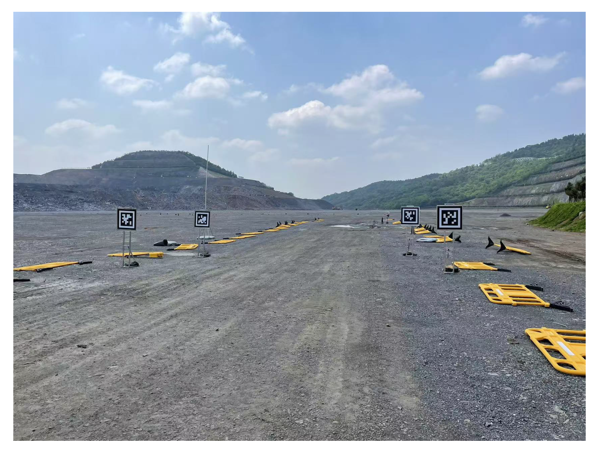

Table A1.
End-to-End Translation Error (meters).
| Dataset | With AprilTag | Without AprilTag |
|---|---|---|
| Campus Test Vehicle | 0.0276 | 0.0922 |
| Mining Heavy Truck | 0.0419 | 0.127 |
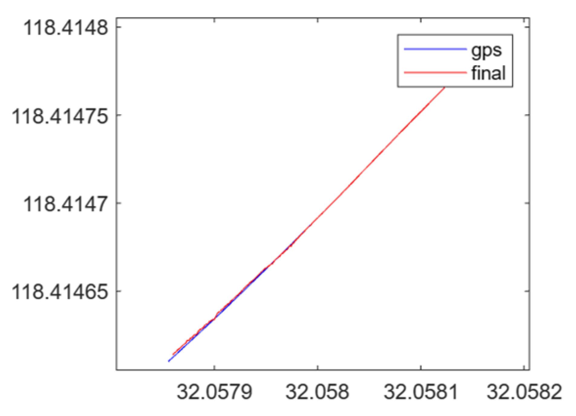
We tested our heavy-duty truck autonomous driving localization module multiple times in mining areas, and the trajectory results are shown in Figure A2. The black shaded areas indicate sections where GPS signals were obstructed. After the autonomous vehicle completed the closed loop, the end-to-end error did not exceed 20 cm, as shown in Figure A3.
Figure A2.
Complete Driving Trajectory Map of the Mining Area.
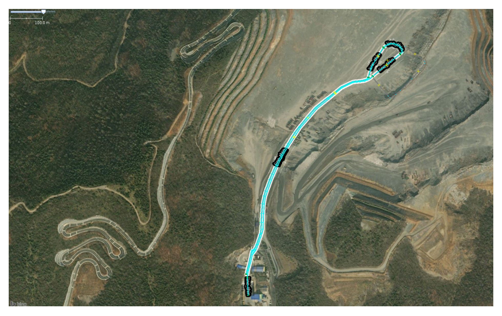
Figure A3.
Complete Driving Endpoint Trajectory in the Mining Area and GPS Ground Truth Trajectory.
References
- A. J. Davison, I. D. Reid, N. D. Molton and O. Stasse, MonoSLAM: Real-Time Single Camera SLAM. IEEE Transactions on Pattern Analysis and Machine Intelligence 2007,vol. 29, no. 6, 1052-1067.
- G. Klein and D. Murray, Parallel Tracking and Mapping for Small AR Workspaces. 2007 6th IEEE and ACM International Symposium on Mixed and Augmented Reality, Nara, Japan, 2007, 225-234.
- R. A. Newcombe, S. J. Lovegrove and A. J. Davison, DTAM: Dense tracking and mapping in real-time. 2011 International Conference on Computer Vision, Barcelona, Spain 2011, 2320-2327.
- Mur-Artal R, Montiel J M M, Tardos J, ORB-SLAM: a versatile and accurate monocular SLAM system. IEEE transactions on robotics 2015, 1147-1163.
- Z. Yuan, J. Deng, R. Ming, F. Lang and X. Yang, SR-LIVO: LiDAR-Inertial-Visual Odometry and Mapping With Sweep Reconstruction. IEEE Robotics and Automation Letters 2024, pp. 5110-5117.
- R. Mur-Artal and J. D. Tardós, ORB-SLAM2: An Open-Source SLAM System for Monocular, Stereo, and RGB-D Cameras. IEEE Transactions on Robotics 2017, 1255-1262.
- C. Campos, R. Elvira, J. J. G. Rodríguez, J. M. M. Montiel and J. D. Tardós, ORB-SLAM3: An Accurate Open-Source Library for Visual, Visual–Inertial, and Multimap SLAM. IEEE Transactions on Robotics 2021, 1874-1890.
- W. Xu, Y. Cai, D. He, J. Lin and F. Zhang, FAST-LIO2: Fast Direct LiDAR-Inertial Odometry. IEEE Transactions on Robotics 2022, pp. 2053-2073.
- T. Shan and B. Englot, LeGO-LOAM: Lightweight and Ground-Optimized Lidar Odometry and Mapping on Variable Terrain. 2018 IEEE/RSJ International Conference on Intelligent Robots and Systems (IROS) 2018, pp. 4758-4765.
- T. Qin, P. Li and S. Shen, VINS-Mono: A Robust and Versatile Monocular Visual-Inertial State Estimator. IEEE Transactions on Robotics 2018, pp. 1004-1020.
- Wei Xu and Fu Zhang, FAST-LIO: A Fast, Robust LiDAR-Inertial Odometry Package by Tightly-Coupled Iterated Kalman Filter. IEEE Robotics and Automation Letters 2020, pp. 3317-3324.
- Li Deren, On Definition,Theory and Key Technics of the Integration of GPS,RS and GIS. Journal of Remote Sensing 1997, pp. 64-68.
- G. Grisetti, C. Stachniss and W. Burgard, Improved Techniques for Grid Mapping With Rao-Blackwellized Particle Filters. IEEE Transactions on Robotics 2007, pp. 34-46.
- S. Kohlbrecher, O. von Stryk, J. Meyer and U. Klingauf, A flexible and scalable SLAM system with full 3D motion estimation. 2011 IEEE International Symposium on Safety, Security, and Rescue Robotics 2011, pp. 155-160.
- Zhang, J., Singh, S, Low-drift and real-time lidar odometry and mapping. Auton Robot 2017, pp. 401–416.
- Mildenhall, B., Srinivasan, P.P., Tancik, M., Barron, J.T., Ramamoorthi, R., Ng, R., NeRF: Representing Scenes as Neural Radiance Fields for View Synthesis. Computer Vision – ECCV 2020 2020.
- Kerbl B, Kopanas G, Leimkühler T, et al. 3D Gaussian Splatting for Real-Time Radiance Field Rendering[J]. ACM Trans. Graph., 2023, 42(4): 139:1-139:14.[Google Scholar].
- Tongyan Hua and Haotian Bai and Zidong Cao and Lin Wang, FMapping: Factorized Efficient Neural Field Mapping for Real-Time Dense RGB SLAM. ArXiv, 2023.
- Vladimir V. Yugay and Yue Li and Theo Gevers and Martin R. Oswald, Gaussian-SLAM: Photo-realistic Dense SLAM with Gaussian Splatting. ArXiv, 2023.
- T. Qin, P. Li and S. Shen, VINS-Mono: A Robust and Versatile Monocular Visual-Inertial State Estimator. IEEE Transactions on Robotics 2018, pp. 1004-1020.
- Zhang Y, Tosi F, Mattoccia S, et al, Go-slam: Global optimization for consistent 3d instant reconstruction Proceedings of the IEEE/CVF International Conference on Computer Vision. 2023, pp. 3727-3737.
- W.Hess,D.Kohler,H.Rapp and D.Andor, Real-time loop closure in 2D LIDAR SLAM. 2016 IEEE International Conference on Robotics and Automation (ICRA) 2016, pp. 1271-1278.
- He, Y.; Zhao, J.; Guo, Y.; He, W.; Yuan, K. PL-VIO: Tightly-Coupled Monocular Visual–Inertial Odometry Using Point and Line Features. Sensors 2018, 18, 1159.
- T. Shan, B. Englot, D. Meyers, W. Wang, C. Ratti and D. Rus, LIO-SAM: Tightly-coupled Lidar Inertial Odometry via Smoothing and Mapping. 2020 IEEE/RSJ International Conference on Intelligent Robots and Systems (IROS) , Las Vegas, NV, USA, 2020, pp. 5135-5142.
- Wang, Han, et al., F-loam: Fast lidar odometry and mapping. 2021 IEEE/RSJ International Conference on Intelligent Robots and Systems (IROS) 2021, pp. 4390-4396.
- T. Shan, B. Englot, C. Ratti and D. Rus, "LVI-SAM: Tightly-coupled Lidar-Visual-Inertial Odometry via Smoothing and Mapping," 2021 IEEE International Conference on Robotics and Automation (ICRA), Xi’an, China, 2021, pp. 5692-5698.
- X. Zuo, P. Geneva, W. Lee, Y. Liu and G. Huang,LIC-Fusion: LiDAR-Inertial-Camera Odometry. 2019 IEEE/RSJ International Conference on Intelligent Robots and Systems (IROS) Macau, China, 2019, pp. 5848- 5854.
- Engel, J., Schöps, T., Cremers, LSD-SLAM: Large-Scale Direct Monocular SLAM. In Computer Vision – ECCV 2014; Fleet, D., Pajdla, T., Eds.; Publishing House: Cham, Switzerland, 2014; pp. 834–849.
- J. Lin;F. Zhang, R3LIVE: A Robust, Real-time, RGB-colored, LiDAR-Inertial-Visual tightly-coupled state Estimation and mapping package, 2022 International Conference on Robotics and Automation (ICRA), Philadelphia, PA, USA, 2022, pp. 10672-10678.
- Wang H, Wang J, Agapito L. Co-slam: Joint coordinate and sparse parametric encodings for neural real-time slam,Proceedings of the IEEE/CVF Conference on Computer Vision and Pattern Recognition. 2023: pp. 13293-13302.
- E. Sucar, S. Liu, J. Ortiz and A. J. Davison, "iMAP: Implicit Mapping and Positioning in Real-Time", 2021 IEEE/CVF International Conference on Computer Vision (ICCV), Montreal, QC, Canada, 2021, pp. 6209- 6218.
- Nikhil Varma Keetha, Jay Karhade, "SplaTAM: Splat, Track and Map 3D Gaussians for Dense RGB-D SLAM", 2024 IEEE/CVF Conference on Computer Vision and Pattern Recognition (CVPR), 2024, pp. 21357- 21366.
- Siting Zhu, Guangming Wang,Hermann Blum, Jiuming Liu, Liang Song,Marc Pollefeys, Hesheng Wang, "SNI-SLAM: Semantic Neural Implicit SLAM", 2024 IEEE/CVF Conference on Computer Vision and Pattern Recognition (CVPR), 2023, pp.21167-21177.
- B. Li, D. Zou, D. Sartori, L. Pei and W. Yu, "TextSLAM: Visual SLAM with Planar Text Features," 2020 IEEE International Conference on Robotics and Automation (ICRA), Paris, France, 2020, pp. 2102-2108.
- evo. Available online: https://github.com/MichaelGrupp/evo (2017).
Figure 1.
The system overvier.
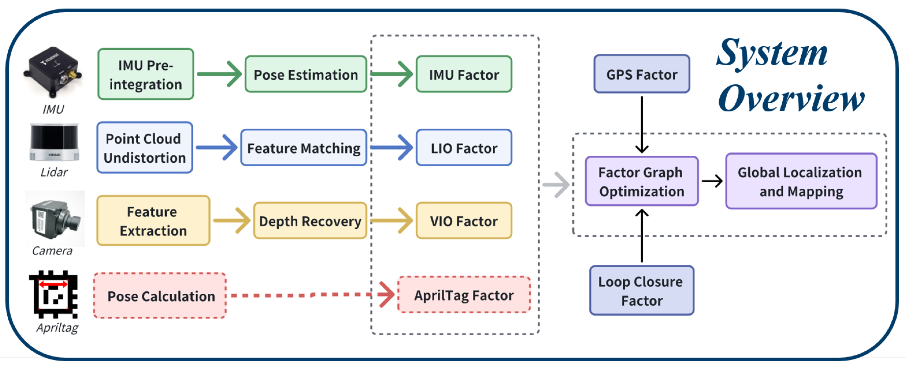
Figure 2.
Illustration of Motion Distortion in Laser Point Clouds.
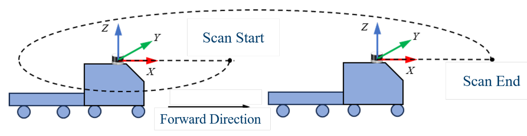
Figure 3.
Point Cloud Undistortion Diagram, where represents the point cloud of the k-th frame and represents the point cloud of the (k+1)-th frame.
Figure 3.
Point Cloud Undistortion Diagram, where represents the point cloud of the k-th frame and represents the point cloud of the (k+1)-th frame.
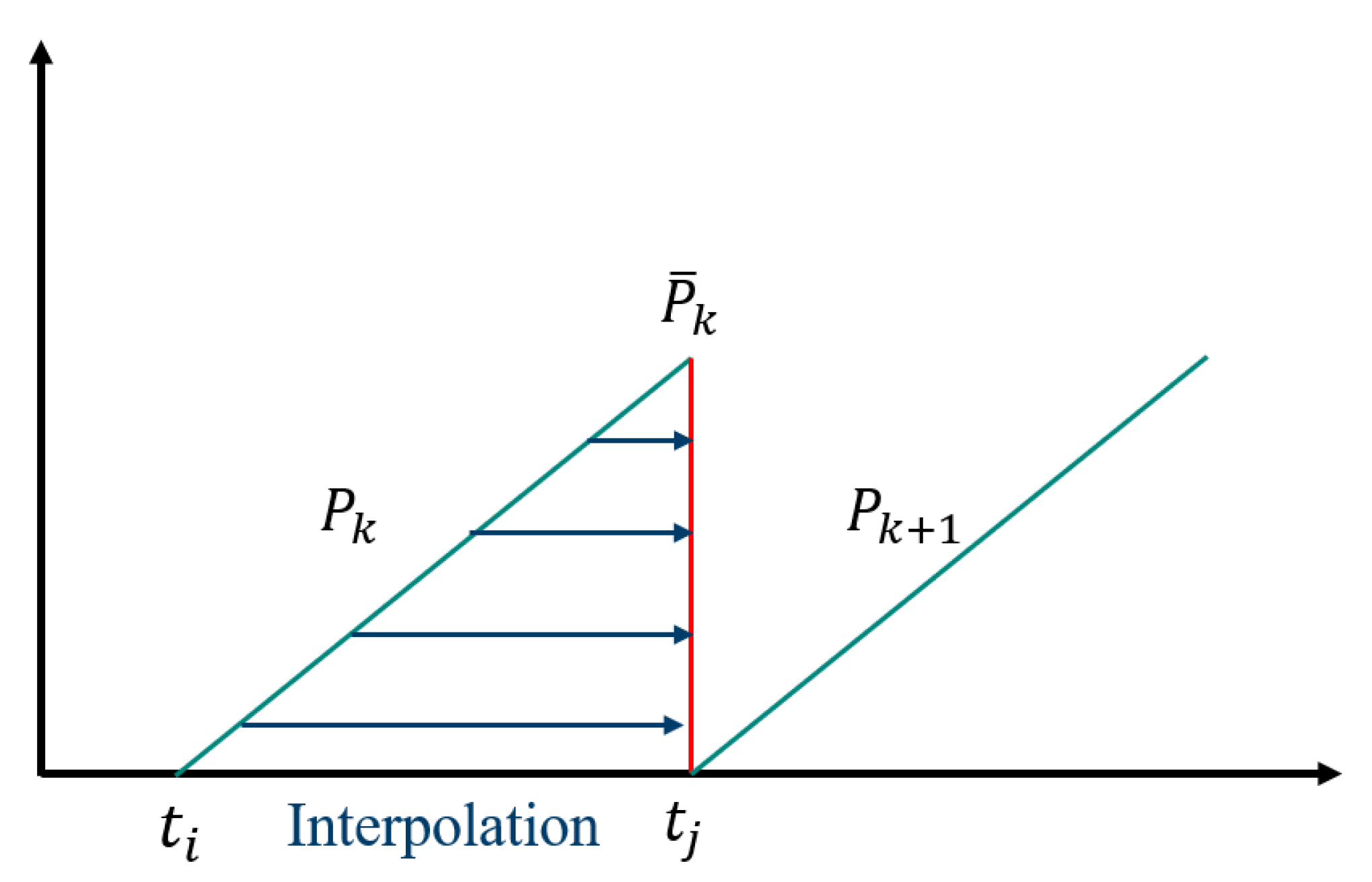
Figure 4.
Schematic Diagram of Laser Keyframes and IMU Pre-integration.
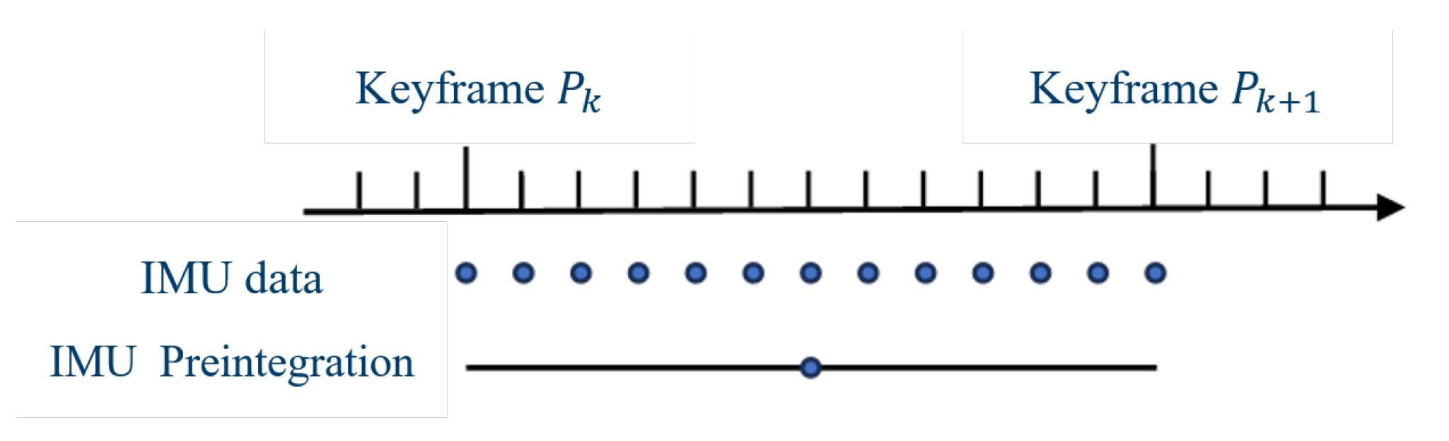
Figure 5.
Time synchronization between point clouds and vision, where is the point cloud output of the k-th frame, is the point cloud output of the k+1-th frame, is the image output of the k-th frame, and is the image output of the k+1-th frame.
Figure 5.
Time synchronization between point clouds and vision, where is the point cloud output of the k-th frame, is the point cloud output of the k+1-th frame, is the image output of the k-th frame, and is the image output of the k+1-th frame.
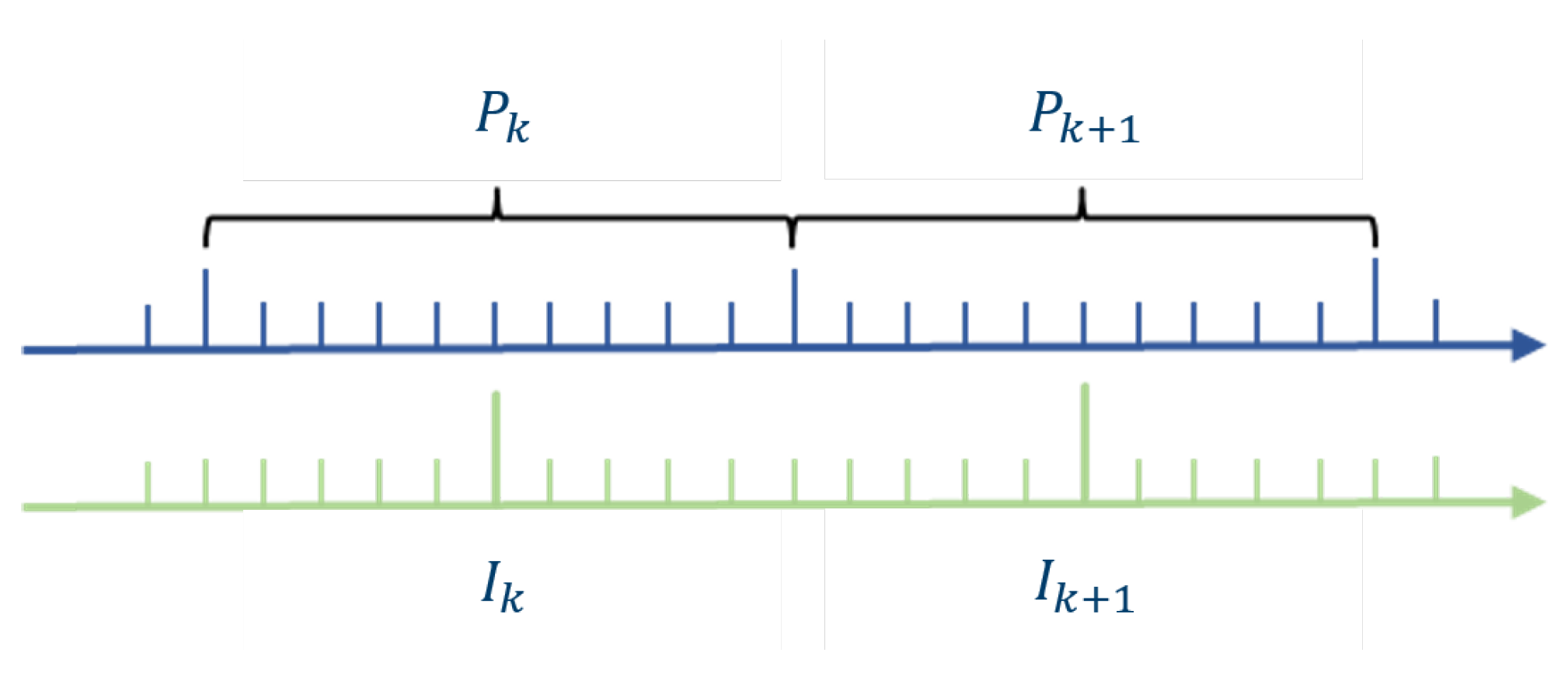
Figure 6.
Schematic Diagram of Factor Graph Optimization Principles.
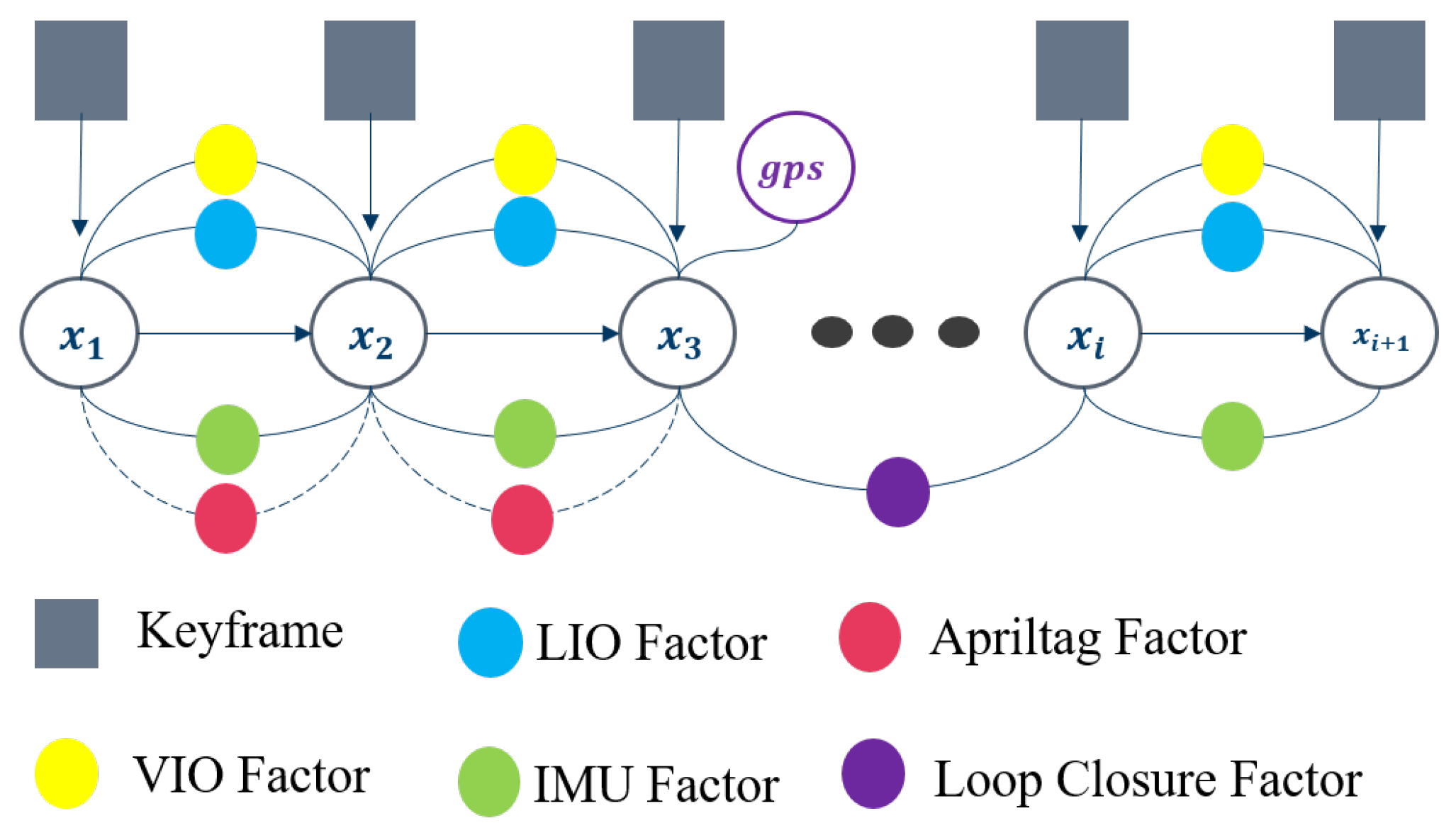
Figure 7.
Algorithm Testing on Public Datasets : (a) Handheld, (b) Garden.
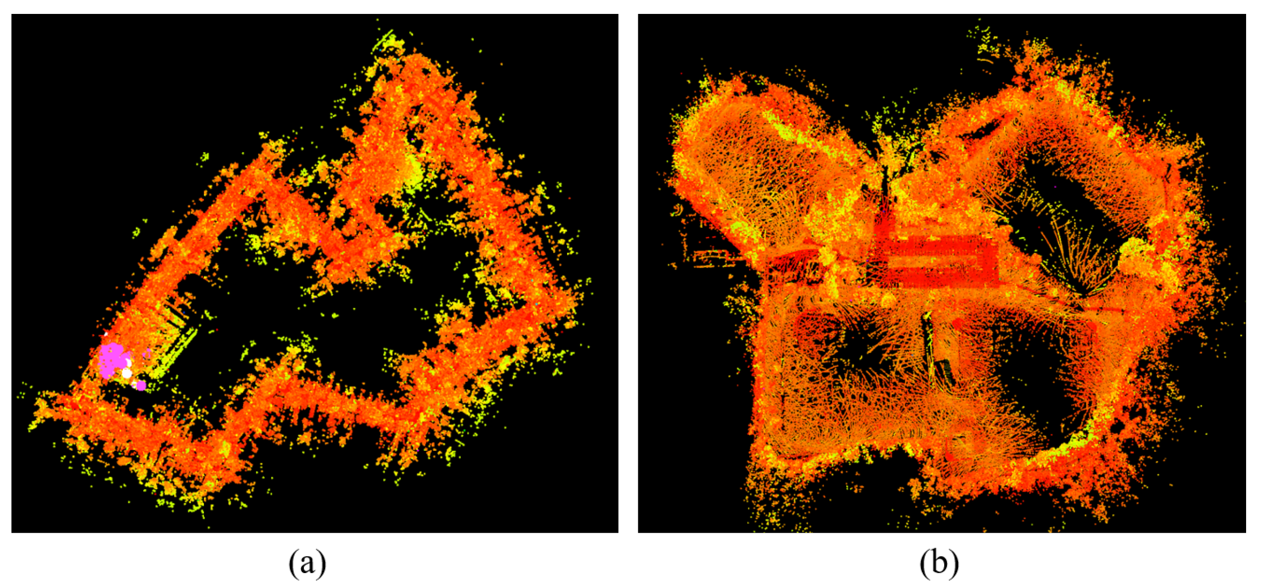
Figure 8.
Test Vehicle and Sensors.
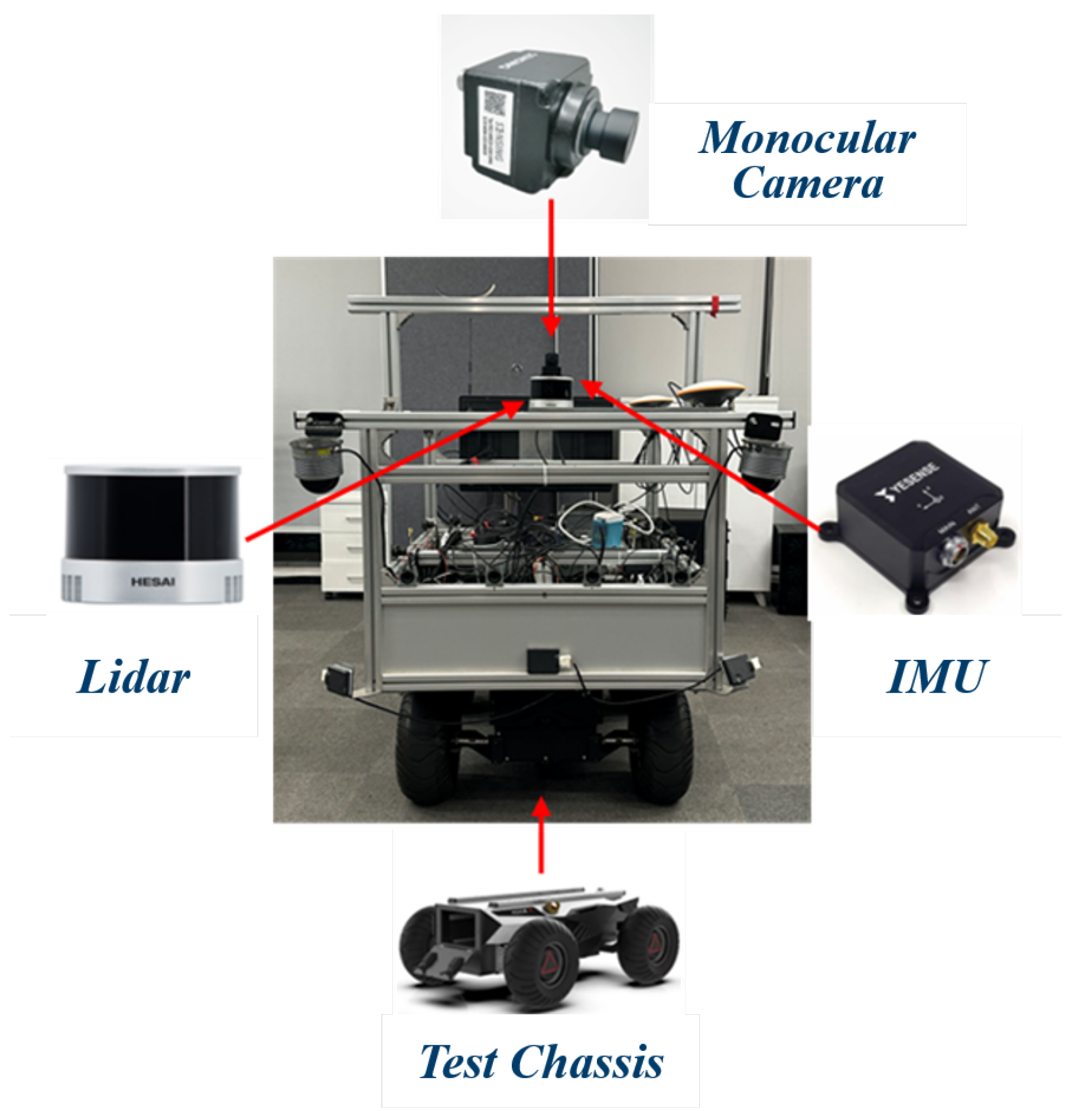
Figure 9.
Trajectory Comparison between Our Localization Method and Ground Truth in the Park Driving Scenario, along with Axis Errors.
Figure 9.
Trajectory Comparison between Our Localization Method and Ground Truth in the Park Driving Scenario, along with Axis Errors.
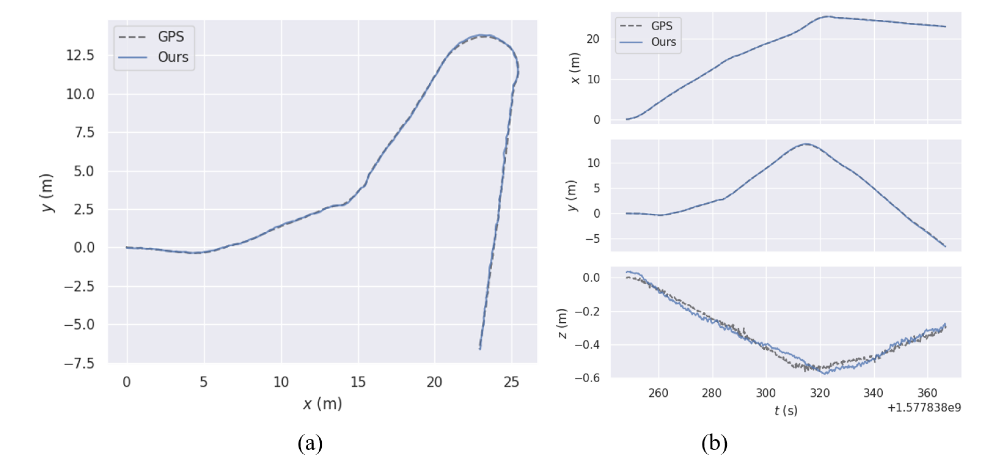
Figure 10.
The satellite image of the mining test area.
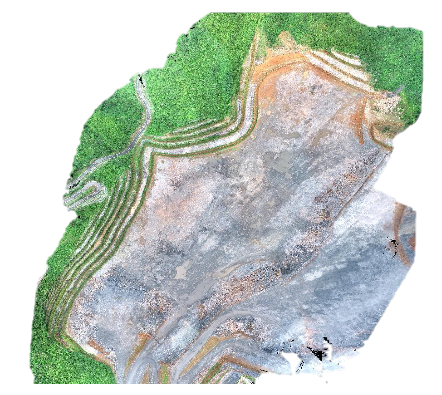
Figure 11.
Heavy-duty Truck and Sensors Used for Autonomous Driving Localization (Left) and Multi-Sensor Fusion Mount (Right).
Figure 11.
Heavy-duty Truck and Sensors Used for Autonomous Driving Localization (Left) and Multi-Sensor Fusion Mount (Right).
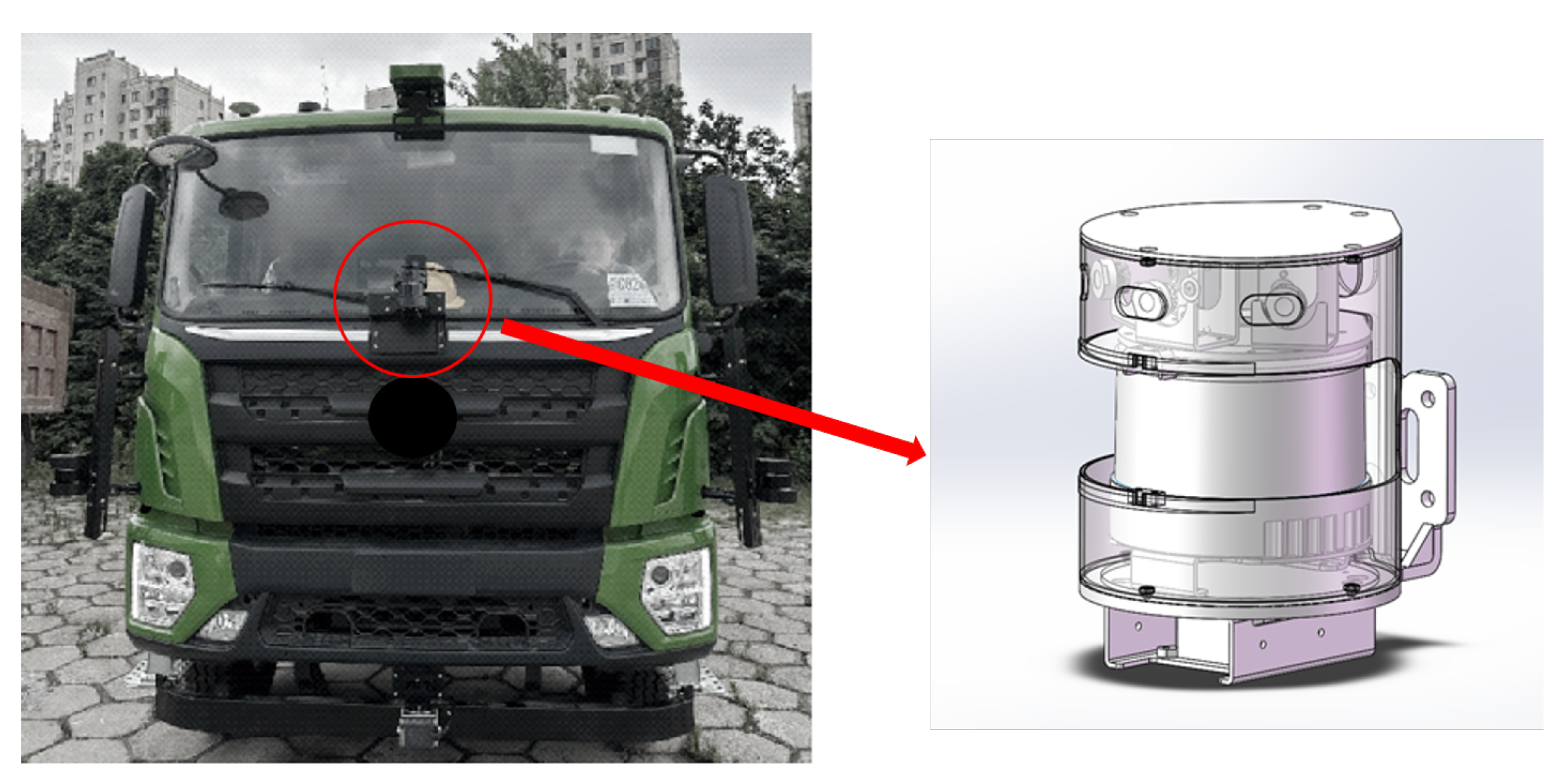
Figure 12.
Comparison of Trajectories for Circular Driving in Heavy Truck Using Our Localization Method and LIO-SAM Against Ground Truth: Trajectory Comparison (a), Axis-wise Error (b) .
Figure 12.
Comparison of Trajectories for Circular Driving in Heavy Truck Using Our Localization Method and LIO-SAM Against Ground Truth: Trajectory Comparison (a), Axis-wise Error (b) .
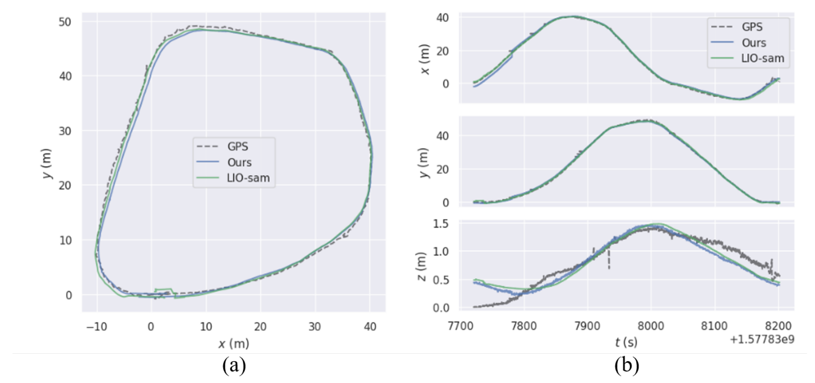
Figure 13.
Statistical Chart of Quantitative Analysis for Heavy-Duty Truck Driving Scenarios.(a) Comparison of APE Error between Two Trajectories and Ground Truth. (b) Box Plot of APE Error between Two Trajectories and Ground Truth.
Figure 13.
Statistical Chart of Quantitative Analysis for Heavy-Duty Truck Driving Scenarios.(a) Comparison of APE Error between Two Trajectories and Ground Truth. (b) Box Plot of APE Error between Two Trajectories and Ground Truth.
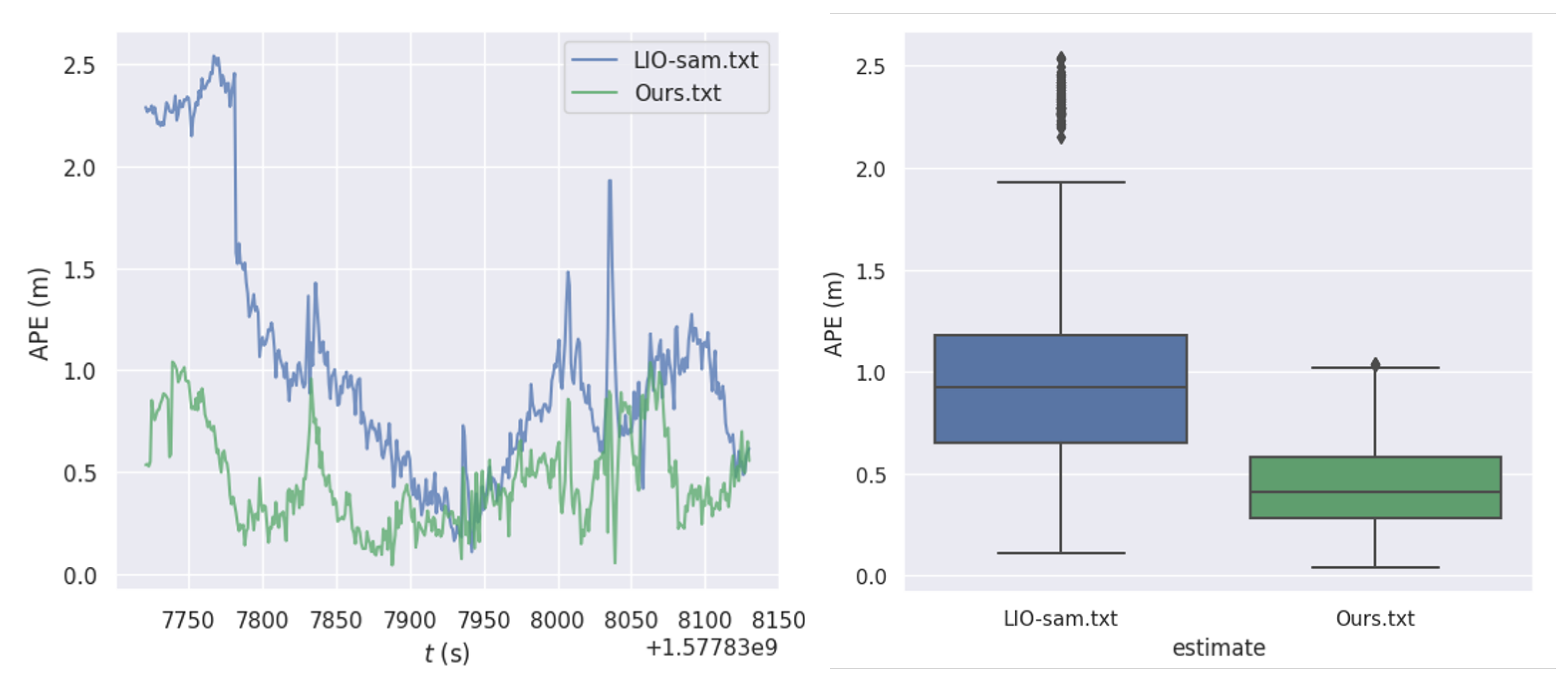
Figure 14.
Comparison of Trajectories for U-Turn Driving in Heavy Truck Using Our Localization Method and LIO-SAM Against Ground Truth: Trajectory Comparison (a), Axis-wise Errorthey (b) .
Figure 14.
Comparison of Trajectories for U-Turn Driving in Heavy Truck Using Our Localization Method and LIO-SAM Against Ground Truth: Trajectory Comparison (a), Axis-wise Errorthey (b) .
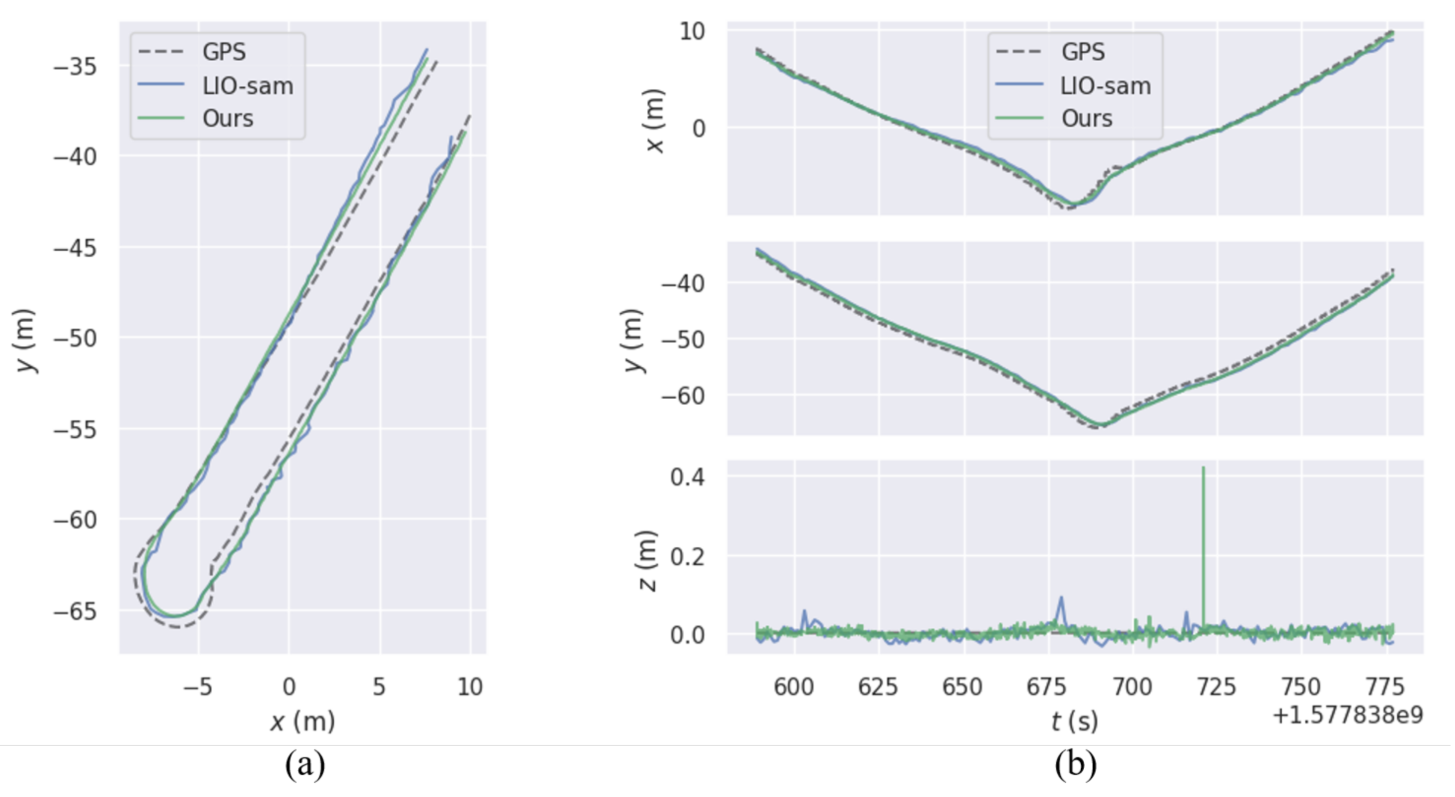
Figure 15.
Statistical Chart of Quantitative Analysis for Heavy-Duty Truck U-Turn Scenarios. (a) Comparison of APE Error between Two Trajectories and Ground Truth. (b)Box Plot of APE Error between Two Trajectories and Ground Truth.
Figure 15.
Statistical Chart of Quantitative Analysis for Heavy-Duty Truck U-Turn Scenarios. (a) Comparison of APE Error between Two Trajectories and Ground Truth. (b)Box Plot of APE Error between Two Trajectories and Ground Truth.
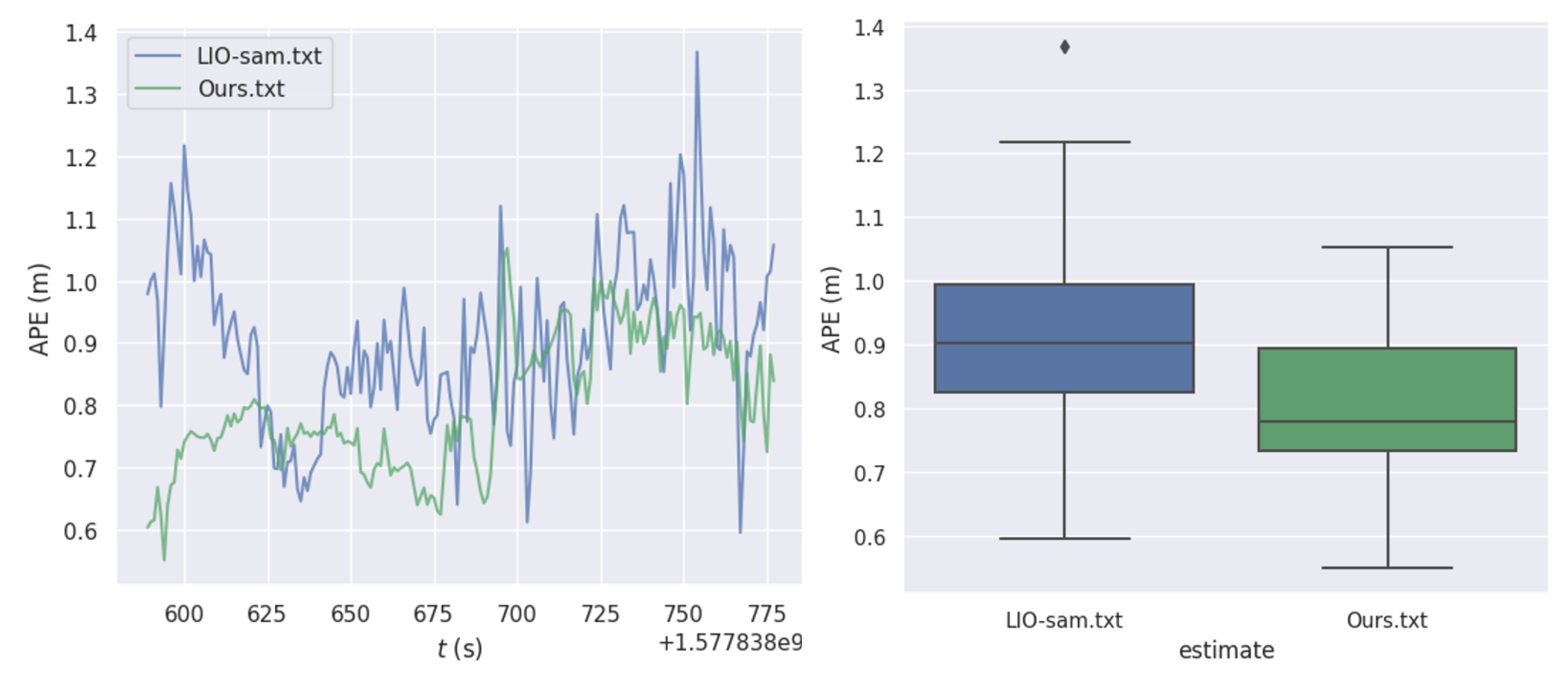
Figure 16.
Schematic Diagram of Algorithm Trajectory Without GPS: (a) Without AprilTag Localization Assistance, (b) With AprilTag Localization Assistance.
Figure 16.
Schematic Diagram of Algorithm Trajectory Without GPS: (a) Without AprilTag Localization Assistance, (b) With AprilTag Localization Assistance.
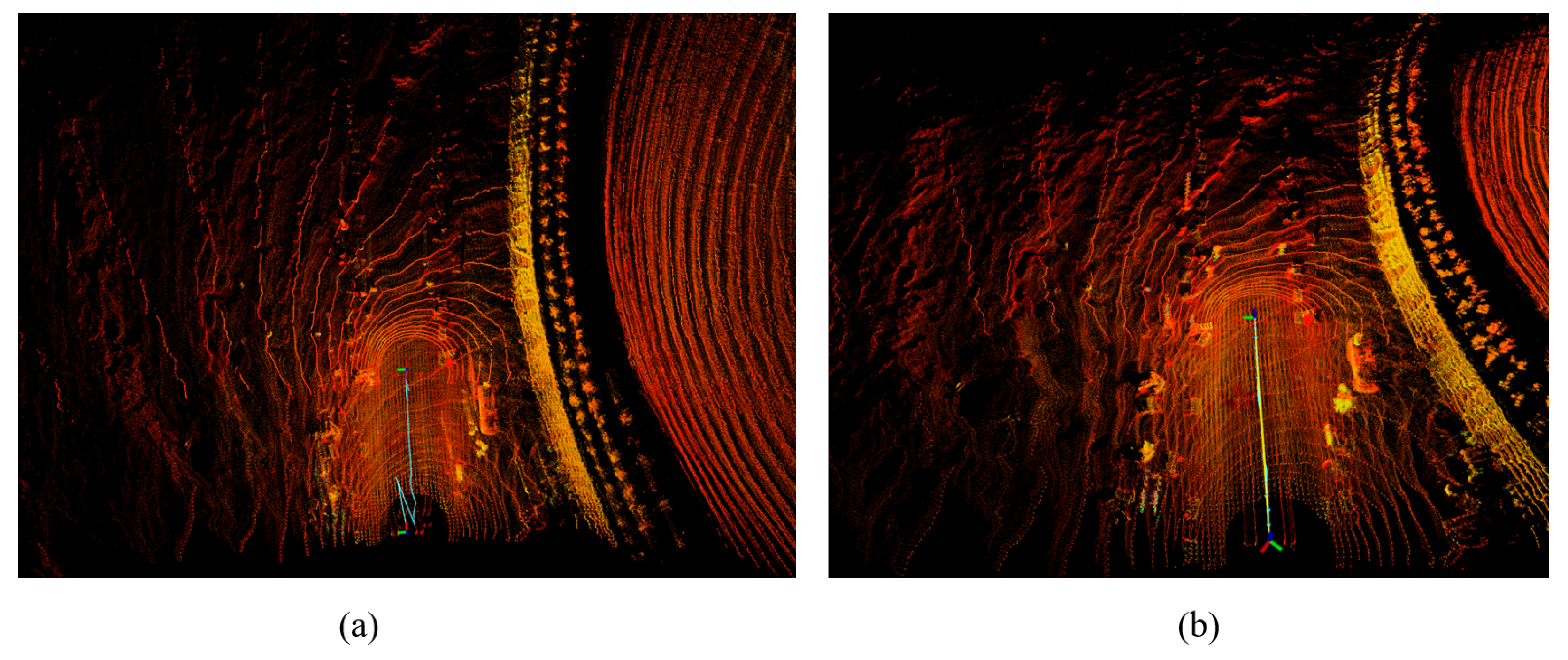
Figure 17.
Schematic Diagram of Algorithm Trajectory : (a) LIO-SAM, (b) Ours.
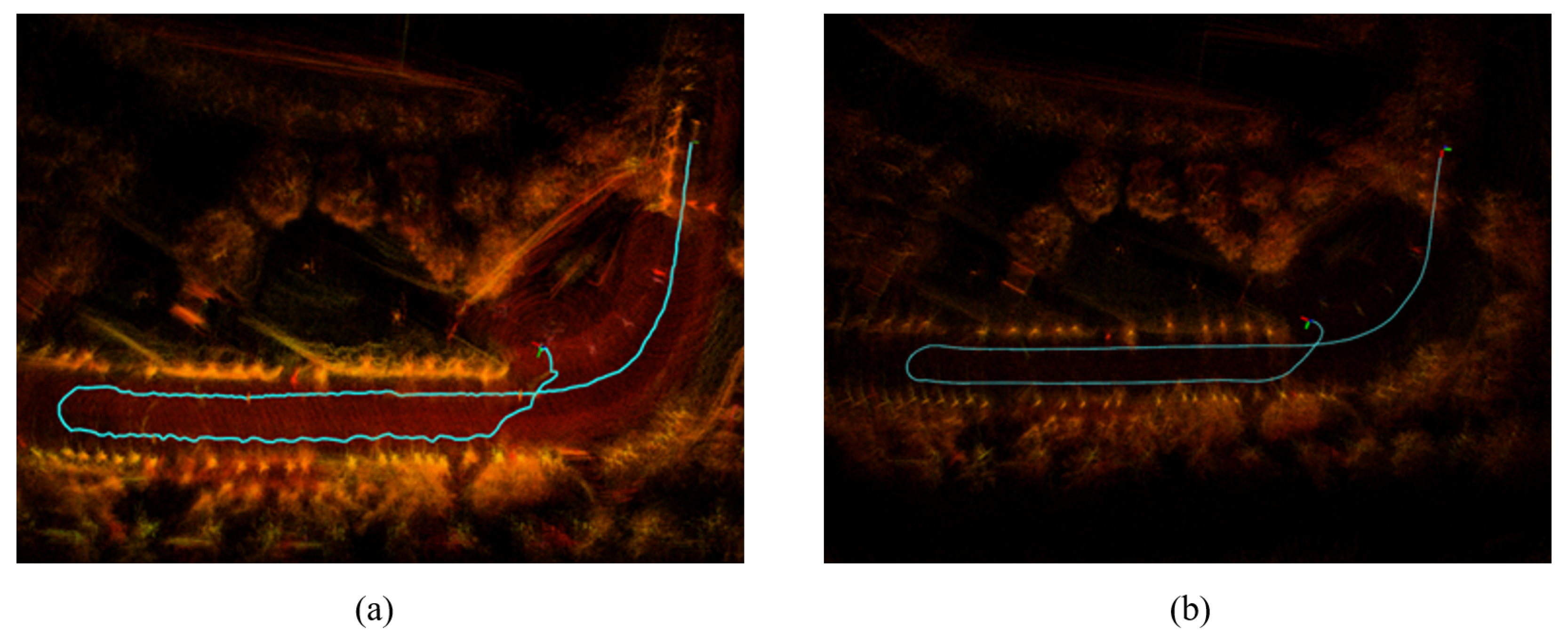
Table 1.
Time Comparison of ikd-tree and kd-tree on Public Datasets (ms).
| Data Structure | Garden | Handle |
|---|---|---|
| kd-tree | 531.264 | 1272.438 |
| ikd-tree | 283.83 | 715.6773 |
Table 2.
Comparison of Algorithm Running Speeds on Public Datasets (frames/s).
| Algorithm | Garden | Handle |
|---|---|---|
| LIO-SAM [24] | 14.8 | 11.3 |
| LVI-SAM [26] | 10.2 | 9.7 |
| Fast-LIO [11] | 15.1 | 12.0 |
| Fast-LIO2 [8] | 17.7 | 18.7 |
| ours | 21.1 | 18.6 |
Table 3.
Running Speed Comparison on the Mining Self-Collected Dataset (Frames/s).
| Method | Circumferential Driving | Turnaround Driving |
|---|---|---|
| LIO-SAM | 23.2 | 22.2 |
| LVI-SAM | 21.7 | 20.6 |
| Fast-LIO | 30.1 | 28.8 |
| Fast-LIO2 | 33.7 | 33.1 |
| Ours | 35.7 | 32.9 |
Table 4.
Quantitative Analysis of Test Results for Different Algorithms on the Heavy Truck Surrounding Driving Dataset(m).
Table 4.
Quantitative Analysis of Test Results for Different Algorithms on the Heavy Truck Surrounding Driving Dataset(m).
| Metric | LIO-SAM | LVI-SAM | Ours |
|---|---|---|---|
| Max Error | 2.541717 | 2.037664 | 1.196394 |
| Mean Error | 1.118793 | 0.983642 | 0.425422 |
| Min Error | 0.106909 | 0.097634 | 0.037963 |
| RMSE1 | 1.276223 | 0.937538 | 0.487019 |
1 Root Mean Square Error.
Table 5.
Quantitative Analysis of Test Results for U-Turn Driving Dataset Across Different Algorithms (m).
Table 5.
Quantitative Analysis of Test Results for U-Turn Driving Dataset Across Different Algorithms (m).
| Metric | LIO-SAM | LVI-SAM | Ours |
|---|---|---|---|
| Max Error | 1.729521 | 1.376932 | 1.052039 |
| Mean Error | 1.051682 | 0.935672 | 0.682019 |
| Min Error | 0.594965 | 0.471874 | 0.321398 |
| RMSE1 | 1.066033 | 0.974323 | 0.697399 |
1 Root Mean Square Error.
Table 6.
Maximum Error between Algorithm Output and Actual GPS at Different Driving Distances(m).
| Trajectory length(m) | LIO-SAM | LVI-SAM | Fast-LIO | Fast-LIO2 | Ours |
|---|---|---|---|---|---|
| 800 | 0.0467 | 0.0324 | 0.0375 | 0.0394 | 0.0108 |
| 3000 | 0.0975 | 0.1291 | 0.0951 | 0.1053 | 0.0276 |
| 10000 | 0.1752 | fail | 0.1632 | 0.1187 | 0.0874 |
| 30000 | fail | fail | fail | fail | 0.1294 |
Disclaimer/Publisher’s Note: The statements, opinions and data contained in all publications are solely those of the individual author(s) and contributor(s) and not of MDPI and/or the editor(s). MDPI and/or the editor(s) disclaim responsibility for any injury to people or property resulting from any ideas, methods, instructions or products referred to in the content. |
© 2024 by the authors. Licensee MDPI, Basel, Switzerland. This article is an open access article distributed under the terms and conditions of the Creative Commons Attribution (CC BY) license (http://creativecommons.org/licenses/by/4.0/).
Copyright: This open access article is published under a Creative Commons CC BY 4.0 license, which permit the free download, distribution, and reuse, provided that the author and preprint are cited in any reuse.


