
Submitted:
02 October 2025
Posted:
03 October 2025
You are already at the latest version
Abstract
The growing demand for sustainable energy alternatives highlights the need for decision-support tools in biodiesel supply chains. This study proposes a mixed-integer programming (MIP) model for tactical planning in the palm oil biodiesel supply chain, focusing on refining, blending, and distribution. The model incorporates economies of scale, inventory, and transport constraints, and is enhanced with valid inequalities (VI) to improve computational efficiency. Computational experiments on simulated instances with up to 6,273 variables and 47 million iterations demonstrated robust performance, achieving solutions within 15 minutes. The model also reduced time-to-first-feasible solutions by 60–75% and CPU times by 17–21% compared to the baseline, confirming its applicability in realistic contexts. The proposed model provides actionable insights for managers by supporting decisions on facility scaling, product allocation, and profitability under supply–demand constraints. Beyond palm oil biodiesel, the approach offers a transferable framework for other renewable energy supply chains where tactical integration and economies of scale are critical.
Keywords:
supply chain
; tactical planning
; mathematical programming
; palm oil
; bio-diesel
1. Introduction
According to the definition of the Council of Supply Chain Management Professionals [8], Supply Chain (SC) management encompasses the planning and management of the activities involved in procurement, conversion and supply, through coordination and collaboration between its links.
One aspect that is still debated worldwide is related to the emission of the carbon footprint that may be generated by the biodiesel supply chains; whether the energy balance of biodiesel is positive, understood as the difference between the energy produced by one kilogram of fuel (biodiesel in this case) and the energy needed to produce it. Another aspect that causes controversy is the impact on the price and availability of food products, fats, oils, among others, derived from agricultural commodities used for biofuel production [7]. Finally, we do not leave aside another controversial aspect, such as environmental care, like monoculture. Despite this, biofuels such as ethanol and biodiesel produced from biomass have been considered worldwide as a real alternative to oil [Dufey, 2006], considering the reduction of world oil reserves, the commitments of countries to reduce their carbon footprint, and the factual evidence of their use at industrial level in oil palm and sugarcane producing countries [5,16] that have favorable conditions for their production such as: high percentage of areas climatically suitable for the cultivation of the commodity and to reach production scales that allow competitive production and logistic costs compared to their alternatives derived from oil [25].
By way of example, in Colombia the State has led the process of promoting biofuels through the proposal and deployment of the national biodiesel policy, established in document CONPES 3510 [12], which has encouraged the production of biodiesel by expanding the percentage of biodiesel in the fuel mix, especially for heavy and cargo transportation. The alternative development and use of biofuels is a reality, showing a growing trend in their production and use, especially because international policies on commodity sustainability have mitigated the negative effects of the crop. In Colombia, production has been increasing since the previous decade due to an increase in demand, which, according to Fedebiocombustibles [13], is expected to continue increasing. The sector is a source of new direct and indirect jobs, it will contribute to the increase of the agricultural GDP in the country, which in 2022, according to Fedebiocombustibles [14], the sector contributed 7.3% and will continue to support the global process of carbon footprint emission mitigation.
These regulatory and public policy frameworks, though relevant, must be translated into tactical tools that enable planning based on profitability and sustainability criteria. This specific need motivates the present work, which addresses a gap in the literature: the absence of integrated mathematical models for the midstream and downstream phases of the biodiesel supply chain in Latin American contexts.
The development of the biodiesel industry calls for development in organizational aspects and in the use of technologies that facilitate its decision-making process, that facilitate planning processes focused on reducing costs along the entire chain and environmental impact to increase its competitiveness and sustainability [17].
This work focuses on addressing deficiencies in the literature that have not conceived the planning of this chain. This work addresses tactical-level planning for the palm-oil biodiesel supply chain’s midstream and downstream (refining, blending, distribution) via a mixed-integer programming model that maximizes after-tax profit under supply–demand, capacity, inventory, and scale-economy constraints.
The paper develops a mixed integer mathematical programming model – MIP and a solution procedure supported by commercial software. The objective of the problem is to maximize after-tax profits. A sensitivity analysis was developed to determine the CPU times for the optimal solutions in practical instances of the problem. Seminal work by Ralphs [27] introduced warm-start mechanisms within integer programming solvers that include capturing the search-tree snapshot—active cuts, variable fixings, branching paths—to resume or accelerate a solve. This demonstrates the foundational tool-level support and theoretical backing for warm-starting capabilities in modern solvers. Warm-start procedures fill this gap by generating feasible incumbents using structured heuristics or previously constructed solutions, thus accelerating solver convergence and complementing the strengths of VI. By merging relaxation strengthening with a warm-start pipeline, our methodology bridges advanced MIP formulation techniques with real-world, scalable solution demands. This alignment is especially pertinent for biodiesel supply chains where decision-makers require feasible solutions early enough to test a variety of demand or capacity scenarios before the full convergence of the solver.
The central research question addressed in this study is: How can tactical-level decisions on refining, blending, and distribution be optimized within a palm oil biodiesel supply chain using a mathematical programming approach that accounts for scale economies and operational constraints?
2. State of the Art
An et al. [3] review mathematical programming models applied to biofuels SC, taking into account the SCM planning levels: Operational, Tactical and Strategic, and the SC stages: Primary (biomass suppliers to conveyor plants), Secondary (Biomass conversion) and Tertiary (storage and customer distribution). The work evidences the dynamics that the biofuels industry has been experiencing on types of biomass and the processes of conversion to biofuels, and concludes that there is a lack of research in the development of support systems for decision making that support a tactical planning that comprehensively manages all the stages that our work addresses.
The following is a review of articles on mathematical programming models that consider the tactical planning of biodiesel SC.

Table 1.
Literature review.
| Reference | Modeling |
|---|---|
| [19] Gonzalez-Negrete et al.(2024) | Title: Optimal planning of oil palm fruit harvest. Objective: Minimize the total costs of the fruit harvesting and transportation operation in an oil palm plantation. Decision Variables: Quantity of raw materials to be collected, lifted and transported. Constraints: Carrying capacity of transport vehicle, size of transport fleet, amount of raw material available for harvesting, market demand. |
| [30] Zhang et al.(2024) | Title: Optimization of biofuel supply chain integrated with petroleum refineries under carbon trade policy. Objective Function: Minimize total SC costs. Decision Variables: Quantity of raw materials to be transported, quantity to be produced, quantity of finished product to be transported. Constraints: Raw material supply capacity, market demand, production capacity. |
| [24] Memari et al.(2017) | Title: An optimization study of a palm oil-based regional bio-energy supply chain under carbon pricing and trading policies. Objective Function: Minimize total cost and carbon emissions. Decision Variables: Quantities to be transported and quantities to be stored. Constraints: Raw material availability, mass balance, storage capacity, reserve limit. |
| [23] Lima et al.(2017) | Title: Stochastic programming approach for the optimal tactical planning of the downstream oil supply chain. Objective Function: Maximize profit. Decision Variables: Import and export costs, Inventory costs, Transportation costs, Inventory quantity, Supply cost, Product quantities processed, Quantity of product exported and imported. Constraints: Processing capacity, Mass balance, Storage capacity, Demand. |
| [18] Ghaithan et al.(2017) | Title: Multi-objective optimization (downstream level) of the oil and gas supply chain. Objective Function: Minimize total supply chain cost and maximize total revenue and service level. Decision Variables: Quantities to produce, Quantities to transport, Inventory levels, Service levels. Constraints: Mass balances, Production capacities, Capacities on each route, Demands, Service Levels, OPEC Quotas. |
| [17] García-Cáceres et al.(2015) | Title: Tactical optimization of the oil palm agribusiness supply chain. Objective: Minimize the operating costs of harvesting and extracting palm oil products. Decision Variables: Material to be transported between the plots and the collection center, Quantity of raw material stored in the plant, Quantity of product stored in the plant, Quantity to be produced, Plant production capacity, Product and raw material storage capacities, Number and type of vehicles used for transport, Number of trips made by each type of vehicle, Number of work teams per zone, Number and type of vehicles, setup (binary). Constraints: Available supply over the planning horizon, Mass balance for each SC node, Production capacity, Storage capacity, Distribution capacity, Distribution infrastructure (in-house and outsourced), Production start-up. |
| [28] Rincón et al.(2015) | Title: Optimization of the Colombian biodiesel supply chain from oil palm crop based on techno-economical and environmental criteria. Objective Function: Minimize total system costs and SC emissions. Decision Variables: Quantity of material flow for each route. Constraints: Biodiesel plant capacity, Biodiesel demand, Quantity of palm oil obtained, Costs. |
| [2] Alfonso-Lizarazo et al.(2013) | Title: Modeling reverse logistics process in the agroindustrial sector: The case of the palm oil supply chain. Objective Function: Maximize the profits obtained from the system. Decision Variables: Quantity in tons of bunches shipped from each hectare of each crop in each vehicle, Quantity in tons of potash shipped from each hectare of each crop in each vehicle, Quantity in tons of fertilizer shipped from each hectare of each crop in each vehicle, Flow between stages of the chain at each harvest, Final inventory at each stage of the chain and at each harvest. Constraints: Flow balance, Capacity, Material balance, Steam demand of each crop, Energy demand of each crop, Inventory balance, Balance of potash and fertilizer, Transport capacity. |
| [4] Avami (2012) | Title: A model for biodiesel supply chain: A case study in Iran. Objective Function: Minimize total SC costs. Decision Variables: Quantity of raw material, Quantity of product to be produced, Quantity of product to be transported. Constraints: Mass balance, Demand, Production capacity. |
| [26] Papapostolou et al.(2011) | Title: Development and implementation of an optimization model for biofuels supply chain. Objective Function: Maximization of the total utility of the chain. Decision Variables: Quantity of production from each grower in each climate scenario, Quantity transported from each grower to the central plant, at each point in time, from each type of storage, in each climate scenario, Capacity of each type of storage, in each time period, from each grower, in each climate scenario, Excess outdoor storage capacity, Shortfall in biomass sent to the central plant. Constraints: Biodiesel demand, Land available for cultivation, Production capacity, Water use, Storage of feedstock and finished product. |
| [9] Cundiff et al.(1997) | Title: A linear programming approach for designing a herbaceous biomass delivery system. Objective Function: Minimization of total supply chain costs. Decision Variables: Biomass flow in the chain at each point in time, Capacity of each type of storage (covered and open storage), Quantity of excess and shortage of biomass. Constraints: Production capacity, Demand, Storage. |
The review shows few works on optimization at the tactical level of direct supply chain (SC) planning for biodiesel and, in particular, for biodiesel produced from palm oil. Regarding decision variables, most of the models reviewed include variables related to product flow—raw materials, intermediate, and finished products through the SC—as well as capacity and mass balance. In recent years, the environmental impact and sustainability of supply chains that integrate both economic and social aspects in strategic contexts have been considered in modeling.
As for the type of modeling, the papers include mixed-integer programming (MIP) and linear programming (LP). There is also evidence of a mathematical programming model for the palm oil agroindustry SC at the tactical level; however, this focuses only on the upstream phase, leaving aside the midstream and downstream phases associated with biodiesel [17]. In addition, there is recent evidence of work on the planning of the oil palm SC operation [19], so the present work is proposed as a complement to these. There is also evidence of SC research on biodiesel from oil palm in reverse flows [2].
In summary, there is no evidence of direct SC optimization models for biodiesel at the tactical decision level, except for the work of Rincón et al. [28], which, however, differs significantly from this study since its purpose is to explore chain expansion under environmental and technological considerations.
Table 2 presents a structured comparison between our proposed model and other recent studies in the field of biodiesel SC optimization. This comparison highlights differences in model type, supply chain scope, objectives, and the unique contributions of each work.
Recent research emphasizes that the effectiveness of mixed-integer programming (MIP) solvers relies heavily on the availability of high-quality incumbent solutions early in the search. In large-scale or complex supply chain problems—such as those IBM has addressed in planning semiconductor supply chains—theoretical models alone are insufficient; heuristic methods that quickly find good feasible solutions are critical to keep computation times acceptable and practical [11].
3. Research Methodology
The research follows a quantitative modeling approach based on operations research principles. A mathematical programming model is formulated to represent the tactical decisions in a biodiesel supply chain. The model structure, assumptions, and constraints are derived from supply chain management literature and adapted to the specific context of palm oil biodiesel. The solution of the model combines two complementary strategies: (i) the inclusion of VI to strengthen the linear relaxation, and (ii) a warm-start procedure designed to accelerate the emergence of feasible solutions and improve the quality of the initial incumbents. The solution procedure is implemented using LINGO 9 and tested on various simulated scenarios with increasing complexity. Model performance is evaluated based on objective value, CPU time, memory usage, and scalability.
Previous works either focus on upstream agricultural logistics or strategic expansion planning. In contrast, this work addresses short-to-medium term planning with tactical detail, offering operational decisions on blending, facility-scale selection, and refined product distribution.
Unlike the previously studied models, this work integrates constraints related to economies of scale, inventories, and multi-level flows in the refining and distribution phases. This integration provides a novel perspective that has been scarcely explored, particularly in models focused on maximizing net profits under real economic parameters.
Our work focuses on the direct planning of SC for decision making, seeking to optimize the flow of materials in the stages and steps of the middle stream and downstream phases based on economic considerations that seek to satisfy the demand in the face of a set of considerations that include: supply, demand, capacity, economy of scale and inventory, and that aims to optimize the net profits of the business units; which together allows the optimization of a multi-agent SC that takes into account the most relevant tactical decisions considered by the literature.
The following is a description of the SC discussed and the development of mathematical programming modeling.
4. The Model
The model is based on the characterization of tactical decisions in refining and blending facilities. It considers the existence of operational scales with increasing economies, mass balances, logistical constraints, and costs associated with product deficits/surpluses. This formulation responds to the need to realistically represent the problem by integrating market and infrastructure conditions.
This paper presents a mathematical programming model for the tactical optimization of the SC of biodiesel from palm oil, seeking to maximize the after-tax profits of the agents involved. The four links comprising the chain under study are: 0. Oil palm fruit suppliers, 1. Extraction plants, 2. Biorefineries, 3. blenders and 4. Demand zones (distributors). Figure 1 illustrates the SC of the biodiesel studied.
To facilitate the reading of the article, parameters are denoted with capital letters and variables with lower case letters. The mathematical programming model developed is presented below:
Indexes and sets:
I: Set of palm fruit suppliers (t: 1, 2, ..);
J: Set of crude palm oil extractors (hereinafter CPO) (t: 1, 2, ...);
Q: Set of diesel biorefineries (t: 1, 2, ..);
K: Set of diesel blenders. (k: 1, 2, ..);
L: Set of demand zones (t: 1, 2, ..);
E: Scales of operation;
EJ(j,b): Operating scales of item b in CPO extractors j, where j Є J;
EQ(q,b): Operating scales of item b in q diesel biorefineries, where q Є Q;
EK(k,b): Operating scales of item b in k diesel blenders, where k Є K;
B: Products;
BI: Set of products supplied by palm fruit suppliers;
BJ: Set of products supplied by CPO extractors;
BQ: Set of products supplied by diesel biorefineries;
BK: Set of products supplied by diesel blenders;
BL: Set of products supplied by demand zones;
Parameters:
FCI: Inventory cycle factor (percentage);
FISJBjb: Safety inventory factor for item b at facility j (Item units / planning period), where j Є J;
FISQBqb: Safety inventory factor for item b at facility q (Item units / planning period), where q Є Q;
FISKBkb: Safety inventory factor for item b at facility k (Item units / planning period), where k Є K;
FJQB(j,q,b): Frequency of trips between CPO extractor j and biorefinery q; of item b;
FQKB(q,k,b): Frequency of trips between diesel biorefinery q and blender k; of item b;
FKLB(k,l,b): Frequency of trips between diesel blender k and demand zone l; of item b;
H: Fraction of inventory holding in a period. Holding cost expressed in $ / ($. Time units). Time units consistent with the average transportation time parameters defined below (generally expressed in $/$. year);
LJQBjqb: Delivery time of item b, de la extractora de CPO i to diesel blender j;
LQKBqkb: Delivery time of item b, from diesel biorefinery j to diesel blender k;
LKLBklb: Delivery time of item b, from diesel blender k to demand zone l;
CFJj: Fixed cost of facility type j in planning period ($ / planning period), where j Є J;
CFQq: Fixed cost of facility type q in the planning period ($ / planning period), where q Є Q;
CFKk: Fixed cost of facility type k in the planning period ($ / planning period), where k Є K;
CFLl: Fixed cost of demand zone l in the planning period ($ / planning period), where l Є L;
CFLBlb: Shortfall cost of item b in demand zone l ($ / item);
CIJBjb: Inventory cost for item b at extraction plant j in the planning period ($ / item);
CIQBqb: Inventory cost for item b in biorefinery q in the planning period ($ / item);
CIKBkb: Inventory cost for item b at blender k in the planning period ($ / item);
CILBlb: Inventory cost for item b in demand zone l in the planning period ($ / item);
CSOLBlb: Cost of surplus of item b in demand zone l ($ / item);
CTIJB(i,j,b): Initial transportation cost of item b to the CPO extractor j provided by palm fruit supplier I;
CTJQB(j,q,b): Initial transportation cost of item b to diesel biorefinery q provided by CPO extractor j;
CTQKB(q,k,b): Initial transportation cost of item b to diesel blender k provided by diesel biorefinery q;
CTKLB(k,l,b): Initial transportation cost of item b to demand zone l provided by diesel blender k;
PLBlb: Selling price of item b in demand zone l ($ / unit of product);
UJBEjbe: After-tax income of item b at extractor j in the planning period ($ / item);
UQBEqbe: After-tax income of item b at biorefinery q in the planning period ($ / item);
UKBEkbe: After-tax income of item b at blender k in the planning period ($ / item);
ULBElbe: After-tax income of item b in demand zone l in the planning period ($ / item);
GMAXJBjbe: Maximum supply of item b provided by CPO extractor j at scale e per planning period (item units / planning period);
GMINJBjbe: Minimum supply of item b provided by CPO extractor j at scale e per planning period (item units / planning period);
GMAXQBqbe: Maximum supply of item b provided by diesel biorefinery q at scale e per planning period (item units / planning period);
GMINQBqbe: Minimum supply of item b provided by diesel biorefinery q at scale e per planning period (item units / planning period);
GMAXKBkbe: Maximum supply of item b provided by diesel blender k at scale e per planning period (item units / planning period);
GMINKBkbe: Minimum supply of item b provided by diesel blender k at scale e per planning period (item units / planning period);
M: A sufficiently large positive number;
Γlb: Demand for item b in demand zone l per planning period (item units / planning period);
Rb1b2: Quantity of item b1 used in the production of item b2 (units by volume or weight of item b1 / item b2 in the extraction plant);
Sb1b2: Quantity of item b1 used in the production of item b2 (units by volume or weight of item b1 / item b2 in the extraction plant);
Bb1b2: Quantity of item b1 used in the production of item b2 (units by volume or weight of item b1 / item b2 in the extraction plant);
TJBjb: Unit transport capacity used by item b between extractor j and biorefinery q (resource units / item);
TQBqb: Unit transport capacity used by item b between biorefinery q and blender k (resource units / item);
TKBkb: Unit transport capacity used by item b between blender k and demand zone l (resource units/item);
CAPPJBjb: Production capacity of extractor plant j, of item b, per planning period (resource units / planning period);
CAPPQBqb: Biorefinery production capacity q, of item b per planning period (resource units / planning period);
CAPPKBkb: blender production capacity k, of item b per planning period (resource units / planning period);
SMAXIBib: Maximum supply of item b provided by supplier i (item units / planning period);
SMINIBib: Minimum supply of item b provided provided by supplier i (item units / planning period);
SMAXJBjb: Maximum supply of item b provided by supplier j (item units / planning period);
SMINJBjb: Minimum supply of item b provided by supplier j (item units / planning period);
SMAXQBqb: Maximum supply of item b provided by supplier q (item units / planning period);
SMINQBqb: Minimum supply of item b provided by supplier q (item units / planning period);
SMAXKBkb: Maximum supply of item b provided by supplier k (item units / planning period);
SMINKBkb: Minimum supply of item b provided by supplier k (item units / planning period);
Decision variables:
xijbe: Quantity of item b supplied by palm fruit supplier i to CPO extractor j at scale e per planning period;
yjqbe: Quantity of item b supplied by CPO extractor j to diesel biorefinery q at scale e per planning period;
zqkbe: Quantity of item b supplied by diesel biorefinery q to diesel blender k at scale e per planning period;
hklbe: Quantity of item b supplied by diesel blender k to demand zone l at scale e per planning period;
wajqbe: Binary variable that takes a value of 1 if item b is produced in extractor j for biorefinery q at scale e per planning period, 0 otherwise;
wbqkbe: Binary variable that takes a value of 1 if item b is produced in biorefinery j for blender q at scale e per planning period, 0 otherwise;
wcklbe: Binary variable taking a value of 1 if item b is produced in blender k for demand zone l at scale e per planning period, 0 otherwise;
gslb+: Amount of surplus of item b in demand zone l;
gdlb-: Quantity in deficit of item b in demand zone l;
Objective function:
Maximize after-tax profit.
where: a*: Pre-tax net income of facility type * in the time period, where * Є (J U Q U K U L).
Net profit of the extractors.
Net profit from biorefineries:
Net benefit of blenders:
Net profit from demand areas (distributors):
Constraints
Scales of operation. Constraints 6 to 8 ensure that the throughput of a facility is associated with that of one of the operating scales at which it can operate.
Constraints 9, 11 and 13 ensure that the facility operates with at most one operating scale. Constraints 10, 12 and 14, on the other hand, limit the amount of throughput of items in each of the operating scales.
Demand: The quantity distributed to a ZD minus its demand generates a demand deficit or surplus.
Production capacity: Constraints 16 to 18 limit the throughput of an item in each facility to the production and handling capacity at the largest scale of operation.
Bill of materials. The raw material used to manufacture the items of a facility cannot exceed the quantity supplied by the suppliers, constraints 19 to 21 model this condition:
Offer. The flow limits per item at each facility or source are modeled by means of constraints 22 to 25. The minimum dimension corresponds to the minimum dimension of the smallest scale of operation and the upper dimension to the maximum of the largest scale of operation of the facility for the specific product:
Finally, the decision variables are non-negative.
5. Solution Procedure
The solution procedure adopted in this study combines two complementary strategies to strengthen the computational performance of the proposed MIP model. First, a set of VI is introduced to tighten the feasible region by exploiting the monotonicity property of economies of scale, thus improving the quality of the linear relaxation. Second, a state-of-the-art warm-start procedure is incorporated to generate high-quality incumbent solutions early in the optimization process. This hybrid approach enhances the ability of commercial solvers to handle large-scale instances by simultaneously improving relaxation strength and reducing the time to obtain feasible solutions, ensuring both efficiency and scalability in the resolution of palm oil biodiesel supply chain planning problems.
5.1. Valid Inequalities
The solution of the model includes a VI proposal stage [29], which has the purpose of bringing the feasible space of the problem closer to its convolution and thus facilitating its solution. VI (26–28) are designed to tighten the feasible region by exploiting the monotonicity property of scale-based production. They are formulated based on the principle that higher-scale operations should not produce lower aggregate flow than smaller ones. Their inclusion improves solution efficiency without affecting optimality.
Scales of production. The VI 26 to 28, in number associated to the number of combinations bounded by the number of scales n: n(n+1)/2 for each of these, were proposed taking advantage of the monotonicity condition of the economies of scales of the production flows of the facilities:
Constraints 29 to 31 ensure that a facility operates, there is flow, only in the event that one of the production scales is activated.
VI indeed tighten the linear relaxation, yet they often fail to yield an immediate feasible solution. The VI propose an adjustment of the feasible region by exploiting the monotonicity property of economies of scale. Equations (26)–(31) formalize this condition. These constraints reduce the gap between the relaxation and the convex hull of the problem without affecting optimality.
5.2. Proposed Warm-Start Solution Procedure
Warm-starting is introduced to cut the Time-to-First-Feasible (TTFF) and improve early optimality gaps, thereby accelerating convergence on large instances. The procedure complements VI by supplying a high-quality incumbent that focuses the branch-and-bound search and reduces node counts. We implement a four-phase pipeline—preprocessing and strong bounds, continuous relaxation with scale mapping, repair LP with feasibility pump if needed, and neighborhood improvement (fix-and-optimize, local branching, RINS)—before launching the global MIP solve with a seeded MIP start.
This procedure aims to generate high-quality incumbent solutions early in the solution process, thereby reducing the computational burden of solving large-scale instances. The procedure is aligned with state-of-the-art approaches in supply chain optimization and consists of four integrated phases:
Phase A – Preprocessing and Strong Bounds. Tight big-M constants are calculated for each scale-product pair based on maximum feasible throughput. Dominated arcs are filtered out, and flow variable bounds are reduced using supply-demand balances and safety stock constraints. This strengthens the LP relaxation before branching.
Phase B – Continuous Relaxation and Scale Mapping. The strengthened LP relaxation is solved without binary variables. The resulting continuous flows are used to map each facility to the smallest operational scale that accommodates its throughput, leveraging the monotonicity property of economies of scale. This generates an initial binary assignment of scales.
Phase C – Repair LP and Feasibility Pump. With binary scale decisions fixed, a repair LP is solved to re-optimize flows. If infeasibility arises due to minimum scale thresholds, a feasibility pump heuristic restricted to scale binaries is applied, followed by another repair LP to restore feasibility. The output is a feasible MIP solution.
Phase D – Neighborhood Improvement. The feasible solution is improved through fix-and-optimize heuristics applied to subsets of facilities, local branching constraints exploring Hamming-distance neighborhoods, and relaxation-induced neighborhood search (RINS). These methods improve the incumbent solution before the global branch-and-bound procedure is launched.
Expected Impact. The warm-start procedure reduces the time to the first feasible solution, decreases the optimality gap in early iterations, and accelerates convergence. It also facilitates the re-use of MIP starts in related instances with perturbed demand or capacity data. Computational experiments should compare baseline results against the warm-start approach to quantify improvements in solution time, optimality gap, and scalability.
Pseudocode of the Warm-Start Procedure. To complement the description of the solution procedure, a pseudocode is provided to outline the warm-start method in an algorithmic manner. This pseudocode aims to facilitate replication of the approach and provides a concise summary of its key steps. The inclusion of this algorithmic representation ensures clarity for both academic readers and practitioners interested in implementing the proposed procedure.
The following pseudocode summarizes the steps of the proposed warm-start procedure, structured into preprocessing, continuous relaxation, repair, and neighborhood improvement. It can be embedded within the solution procedure section to provide a clear, algorithmic description of the approach for reproducibility and implementation.
- WS-PalmBiodiesel():;
- A) PreprocessAndTighten();
- Compute tight big-M or replace with SOS1/indicator constraints;
- Remove dominated arcs and tighten flow bounds by supply-demand balances;
- B) (x̄,ȳ,z̄,h̄) ← SolveContinuousRelaxation (with VI);
- w* ← MapScalesGreedyMonotone (throughputs from x̄,ȳ,z̄,h̄);
- C) (x*,y*,z*,h*) ← RepairLPGivenScales(w*);
- if infeasible:;
- (w*,x*,y*,z*,h*) ← FeasibilityPumpRestrictedTo(w) → RepairLP;
- D) Incumbent ← (w*,x*,y*,z*,h*);
- LoadAsMIPStart(Incumbent);
- ImproveByFixAndOptimize(Blocks);
- LocalBranching(k);
- RINS();
- return Incumbent;
The pseudocode highlights the structured sequence of the warm-start procedure, from preprocessing and continuous relaxation to repair and neighborhood improvement. By following this structure, researchers and decision-makers can reproduce the method, adapt it to related biofuel supply chain models, and extend it with metaheuristics or decomposition techniques. This structured description bridges the conceptual explanation of the solution approach with the empirical results presented in the next section.
Warm-Start Solution Procedure — LINGO. This procedure to implement the warm-start pipeline in four stages: (1) LP relaxation of the strengthened model, (2) scale mapping from continuous throughputs, (3) repair LP with scales fixed, and (4) full MIP solve seeded with the repaired solution (MIP start).
Key Parameters (Symbols & Roles). The table shows the factors that control relaxation strength and incumbent construction: scale bounds (GMIN/GMAX), capacity settings (CAPP), and penalty parameters (CFLB/CSOLB). Careful tuning of these values helps achieve lower TTFF and smaller early gaps.
Table 3.
Key Parameters.
| Symbol | Description | Type | Domain |
|---|---|---|---|
| GMAX* | Maximum throughput at scale e | Parameter | ℝ₊ |
| GMIN* | Minimum throughput at scale e | Parameter | ℝ₊ |
| CAPP* | Facility capacity (resource units/period) | Parameter | ℝ₊ |
| FIS* | Safety stock factor | Parameter | ℝ₊ |
| H | Inventory holding fraction | Parameter | ℝ₊ |
| CT* | Initial transport cost | Parameter | ℝ₊ |
| CI* | Inventory cost | Parameter | ℝ₊ |
| CSOLB | Surplus penalty | Parameter | ℝ₊ |
| CFLB | Shortage penalty | Parameter | ℝ₊ |
| PLB | Selling price at demand zone | Parameter | ℝ₊ |
| x,y,z,h | Flows between stages | Variable | ℝ₊ |
| w | Scale-activation binaries | Variable | {0,1} |
| g⁺, g⁻ | Surplus / shortage | Variable | ℝ₊ |
6. Solution and Results
Warm-starting is used to cut TTFF and early gaps, focusing the branch-and-bound search and reducing node counts on larger instances. Our four-phase pipeline—(A) preprocessing and strong bounds, (B) continuous relaxation with scale mapping, (C) repair LP with a restricted feasibility-pump if needed, and (D) neighborhood improvement (fix-and-optimize, local branching, RINS)—produces a high-quality incumbent that is loaded as a MIP start before the global solve.
An analysis was performed on commercial LINGO 9 software operated on an Intel Core I5, 2.67 Ghz CPU with 8GB of RAM and a 64-bit operating system (Windows 10). For integrality checks, we used LINGO’s absolute and relative integrality tolerances ABSINT = 1e−6 and RELINT = 8e−6, respectively, so that an integer variable x is deemed feasible when ∣x−I∣≤ 1e−6 or ∣x−I∣/∣x∣≤ 8e−6. Linear feasibility tolerances followed the standard ILFTOL/FLFTOL settings (≈ 3e−6 and 1e−7), and the linear optimality tolerance LOPTOL was kept at 1e−7. Early termination of the MIP search was governed by the relative optimality tolerance IPTOLR (relative gap).
LINGO 9 was selected due to its built-in support for solving MIP problems with VI and for its ease of integration with algebraic modeling languages. Although LINGO offers acceptable computational performance, the model remains NP-hard due to binary decision variables and flow constraints, which can affect scalability beyond certain instance sizes. Additionally, the model formulation is compatible with other commercial solvers such as CPLEX, Gurobi, or GAMS, offering flexibility for implementation depending on user preferences or computational resources.
The tested instances reflect realistic network sizes for tactical planning in palm-oil biodiesel, spanning 814–6,273 variables and up to ~1.8×10⁴ constraints, which aligns with mid-scale industrial studies. The model parameters were analyzed in three different instances, including VI. Table 4 presents the SC configuration.
Performance comparing the baseline solve with the warm-start pipeline. For warm start we also report standard deviations across 10 runs. Table 5 complements the network configuration in Table 4 and the solver/tolerance settings described above, enabling an integrated view of scalability and solver efficiency [6,10,15]
Overall, the results highlight three clear patterns. First, problem scale increases significantly across instances (e.g., 814→6,273 variables; ~1.4k→17.7k constraints), reflected in a non-linear growth of iterations (≈1.6×10⁴→4.7×10⁷). Second, the warm-start procedure reduces TTFF by 60–75% and CPU time by ≈17–21%, with relative gains that persist or improve as the instance size grows (e.g., in Instance 4, CPU decreases from ~10,153 s to ~8,000 s, ≈21.2%). Third, profit values are not monotonic with problem size (Instance 2 exceeds Instances 1 and 4), which is consistent with structural differences in parameterization and network topology rather than algorithmic performance. Importantly, TTFF values are consistently lower than CPU times, as theoretically expected, and the reported standard deviations show moderate variability across 10 runs. These findings align with prior studies reporting the stabilizing role of warm starts in mixed-integer programming [1,22].
The observed computational gains are consistent with prior findings on primal heuristics and warm-start procedures in mixed-integer programming. In particular, early incumbents generated by approaches such as Feasibility Pump and relaxation-induced neighborhood search tend to shrink initial gaps and reduce node counts, which in turn accelerates convergence [6,10,15]. The magnitude and pattern of TTFF reductions in our experiments (60–75%) fall within the upper range reported for problems where the number of binaries and the breadth of the search tree amplify the value of high-quality incumbents. Moreover, the larger absolute savings in medium-to-large instances agree with solver behavior documented on representative test sets such as MIPLIB 2010, where the impact of incumbents generally increases with problem scale and complexity [1,22].
Across 10 independent runs per instance, the dispersion of warm-start performance is modest in absolute terms and shrinks, in relative terms, as problem size grows. For TTFF, standard deviations of 0.3/1/45/90 s yield coefficients of variation (CV) of ~30.0%, 16.7%, 14.3%, and 12.5% for Instances 1–4, respectively. For CPU, standard deviations of 5/7/45/80 s correspond to CVs of 100%, 14%, 2.0%, and 1.0%. The inflated CV for Instance 1 is purely a denominator effect (mean CPU = 5 s); in practical terms, a ±5 s spread is negligible. For the largest instance, the 95% confidence interval of the warm-start CPU mean is approximately 8,000 ± 60 s (n = 10), reinforcing stability. This pattern—lower relative variability as scale and search-tree breadth increase—is consistent with the behavior of primal-heuristic–aided solves reported in the MIP benchmarking literature, where high-quality incumbents reduce sensitivity to random seeds and cut activation order [1,6,22].
It can be deduced from the previous table that the TTFF and CPU times for the solution of the different instances of the problem show good performance values for the instances under study. The summary of the runs of instance 1 is presented in order to better illustrate the results, see Table A1. The results of the four instances also are presented in Appendix A.
Table A1 disaggregates the optimal solution for Instance 1 across the four stages—suppliers → extractors → biorefineries → blenders → demand zones—thus illustrating how the model operationalizes economies of scale and mass-balance consistency. Four patterns stand out:
Network Sparsity with Cost-Driven Routing
Flows concentrate on a limited set of i→j, j→q, and q→k arcs, indicating that the solver selects a small number of cost-effective routes while suppressing dominated arcs identified in preprocessing. This sparsity is consistent with the fixed/initial transport cost structure and leads to lower effective unit costs at activated routes (cf. constraints 22–25).
Scale Activation Consistent with Throughput
Although scale binaries are not shown in Table A1, the throughputs implied by x, y, z, and h align with the monotonicity logic enforced by the VI: facilities operate at the smallest scale that feasibly accommodates their load, avoiding minimum-scale infea-sibilities and capturing scale economies where volumes justify it (constraints 6–14 and VI 26–31).
Mass-Balance Coherence and Capacity Discipline
The observed stage-to-stage throughputs are coherent with bill-of-materials relations and do not overshoot facility produc-tion/handling limits, reflecting compliance with capacity constraints (16–18) and input–output balances (19–21). This ensures that the material flow plan is physically implementable without artificial slack.
Service Levels Priced By Penalty Terms
Deliveries from blenders to demand zones (h) prioritize meeting market requirements; any residual imbalance is priced via shortage/surplus penalties rather than hidden in the flow structure (constraint 15 and parameters CFLB/CSOLB). In the reported solution, these penalties are non-dominant in the profit decomposition (constraints 2–5), confirming that profitability is primarily driven by scale-efficient processing and cost-effective routing.
Managerial Takeaway
Even in a small network, the model (i) channels volume through a few high-leverage routes and scales, (ii) respects plant bot-tlenecks, and (iii) keeps imbalance penalties marginal. Practically, this means that managers can increase profitability by (a) consolidating flows on the most economical corridors, (b) activating facility scales only when throughput clears minimum thresholds, and (c) monitoring bottlenecks at extractors and refineries where marginal capacity expansions yield the largest gains.
Sensitivity Analysis
A sensitivity analysis was performed to evaluate the impact on the objective function, derived from eventual changes in certain parameters of the model. The results can significantly help in the decision-making process in the entire SC. Thresholds of change in the study parameters were selected at a value sufficient to clearly identify the effects on the utilities. In this regard, the analyses studied the impact of changes between 10% and 90% with 10% increments. The simulated parameters were revenues and capacities for each of the facilities in order to study the effect of the change on profits (objective function).
Impact of Revenues on Profits
Figure 3 details the impact of revenues on profits for each of the links, constraints 2 to 5, which shows a linear behavior in all cases.
Increases in revenues lead to non-negative and significantly higher percentage variations in profits in each of the links and facilities analyzed, which shows the goodness of profit derived from focusing on higher revenues as long as the other parameters do not vary significantly, a matter of interest for SC managers.
The revenue and capacity sensitivities translate into actionable rules for tactical planning. On the revenue side, the near-linear response of profits (cf. constraints 2–5) implies that managers should prioritize commercial actions that raise effective selling prices or net unit revenues at refineries and blenders, where the slope of the profit curve is steepest in our tests. On the capacity side (constraints 16–18), the increasing but diminishing marginal gains indicate a practical expansion threshold: invest in additional capacity (or activate a higher operating scale) only when expected throughputs approach the current scale’s lower bound (GMIN*) and the marginal profit still exceeds the shadow cost of capacity. In operational terms, (i) consolidate flows on corridors already operating at favorable scale, (ii) upgrade scale at extractors/refineries before persistent bottlenecks force costly rerouting or shortages (CFLB), and (iii) keep surplus penalties (CSOLB) non-dominant by aligning production plans with demand zones that exhibit the highest revenue elasticity. Because the marginal returns flatten beyond the first capacity increments, further expansions should be justified by scenario runs (e.g., demand or price shocks), which the warm-start pipeline can evaluate rapidly through MIP-start reuse across perturbed instances.
Impact of Capacities on Profits
Figure 4 details the impact of capacities on profits for each of the links, which shows an increasing non-linear behavior in all the SC links.
The study of the impact on profits caused by the increase in capacity of the related parameter in each of the constraints 16 to 18. With the increase in capacity of each facility, positive and marginally decreasing percentage variations in profit are observed in each of the analyzed links. The results show that the effects on utility are slightly higher in percentage terms in the refining and final distribution stages and slightly lower in the other two stages of the SC; this is explained by the fact that the stages do not experience the same level of marginal exploitation of economies of scale.
The analyses can be extended to other parameters such as cost components, which, however, are usually kept confidential by the companies and are beyond the scope of this work, which does not imply that they can be taken into account by decision-makers.
In addition to revenue and capacity variations, future analyses may incorporate sensitivity to unit transportation costs, energy prices, and carbon penalties—factors with significant real-world variability and strategic implications.
Taken together, the experiments show consistent TTFF and CPU improvements from coupling VI with a warm-start pipeline, with stable dispersion across 10 runs per instance and increasing relative benefits as instance size grows. The disaggregated flows confirm feasibility, scale-activation logic, and cost-driven routing, while the sensitivity tests supply actionable levers—pricing, scale upgrades, and corridor consolidation—and support rapid scenario evaluation via MIP-start reuse. We now synthesize managerial implications and outline methodological extensions in the Conclusions.
7. Conclusions
This paper contributes to the development of tactical-level optimization models by incorporating production and distribution planning in a unified MIP framework for biodiesel derived from palm oil. It addresses a specific research gap by explicitly modeling midstream and downstream flows with VI and scalable production decisions.
The boost given to the biofuels option in recent years has positioned it as a real alternative to reduce CO₂ emissions and mitigate climate change. The effort to optimize and make the industry sustainable implies the development of decision support systems, which follows a line of works that are consolidating a dossier of technical possibilities that facilitate the management of the SC.
This work proposes a MIP mathematical programming model and a solution procedure based on VI that was supported in a commercial solver to tactically optimize the SC of biodiesel (at midstream and downstream levels) and can be assumed as complementary work to the efforts undertaken for the upstream phase of the oil palm supply chain. The model is based on the characterization of tactical decisions in refining and blending facilities. It considers the existence of operational scales with increasing economies, mass balances, logistical constraints, and costs associated with product deficits/surpluses. This formulation responds to the need to realistically represent the problem by integrating market and infrastructure conditions.
Research perspectives are focused on two fronts: the first one is algorithmic, to make its solution more efficient, supported by relaxations such as Benders or Column Generation or by the development of heuristics if the algorithmic solution is insufficient. The second front is related to the inclusion of new constraints or objectives.
From a managerial perspective, the model can support decisions on facility scaling, product allocation, and economic feasibility under supply-demand constraints. However, the current approach assumes deterministic demand and cost data, which limits its application in uncertain environments. Future work should consider stochastic formulations and real-time data integration.
The computational analysis performed in this work was aimed at determining the efficiency of the problem under the objective of maximizing after-tax profits. The TTFF and CPU times obtained for the optimal solution showed a good performance in practical instances of the problem. From a computational perspective, the integration of VI and warm-start mechanisms proved to be a robust strategy for tactical-level biodiesel supply chain problems under economies of scale. Across all instances, substantial reductions were observed in TTFF (60–75%) and CPU time (≈17–21%), with bounded dispersion across runs. These results confirm that providing an early high-quality incumbent guides a more focused branch-and-bound search, accelerates gap closure, and improves scalability without altering model optimality [10,15].
Managerial implications and future work. The model supports decisions on facility scaling, product allocation, and economic feasibility under realistic supply-demand constraints, with computation times compatible with tactical “what-if” analyses. Future extensions should include (i) stochastic formulations addressing demand, cost, and energy-price uncertainty; (ii) decomposition-based approaches (Benders, column generation) and lightweight metaheuristics for large-scale instances; and (iii) reuse of MIP starts under perturbed input data, leveraging the warm-start pipeline to accelerate sensitivity analyses and scenario planning [6,22].
Results are based on simulated data and a single commercial solver on mid-range hardware, which may limit generalizability to larger industrial networks. Deterministic parameters omit demand and price uncertainty; however, the warm-start pipeline facilitates rapid “what-if” re-solves under perturbed scenarios. Cross-solver tests (e.g., CPLEX/Gurobi) and stochastic extensions are left for future work.
The approximation of the problem that has been presented can be a basis for further work both in mathematical modeling with the inclusion of new constraints and objectives as well as the development of solution procedures based on heuristics and/or metaheuristics, to be compared considering optimality gaps, memory usage, computational time, among other performance parameters.
Theoretically, this model contributes to the literature by integrating multi-stage tactical planning and valid inequality techniques in palm oil biodiesel SCs—offering a framework adaptable to other renewable energy sectors.
Author Contributions
Conceptualization, R.G.G.-C., O.R.B.-R. and C.M.-M.; methodology, R.G.G.-C.; software, O.R.B.-R.; validation, R.G.G.-C., O.R.B.-R. and C.M.-M.; formal analysis, R.G.G.-C.; investigation, R.G.G.-C.; resources, R.G.G.-C.; data curation, O.R.B.-R.; writing—original draft preparation, R.G.G.-C.; writing—review and editing, C.M.-M.; visualization, C.M.-M.; supervision, R.G.G.-C.; project administration, R.G.G.-C.; funding acquisition, R.G.G.-C. All authors have read and agreed to the published version of the manuscript.
Funding
This research received no external funding.
Data Availability Statement
The data that support the findings of this study are available from the corresponding author upon reasonable request.
Acknowledgments
The authors thank the Universidad Pedagógica y Tecnológica de Colombia (UPTC) for institutional support and academic resources that supported the completion of this research.
Conflicts of Interest
The authors declare no conflict of interest. The funders had no role in the design of the study; in the collection, analyses, or interpretation of data; in the writing of the manuscript; or in the decision to publish the results.
Appendix A
Appendix two presents the results of the decision variables for instance 2 and instance 3 of the problem.
Table A1.
Results of instance 1.
| xij1 : Quantity of the item supplied by supplier i to extractor j. | yjq1 : Quantity of the item supplied by extractor j to biorefinery q. | ||||||
| i j | 1 | 2 | 3 | j q | 1 | 2 | 3 |
| 1 | 648 | 0 | 1008 | 1 | 100.666667 | 268 | 387 |
| 1 | 648 | 0 | 0 | 1 | 0 | 0 | 0 |
| 1 | 573.269231 | 0 | 0 | 1 | 186 | 93 | 0 |
| 1 | 398.333333 | 0 | 0 | 1 | 0 | 0 | 223 |
| 1 | 0 | 703 | 0 | 2 | 355 | 290.140276 | 301 |
| 2 | 896 | 776.333333 | 610.666667 | 2 | 283.790293 | 0 | 0 |
| 2 | 517.249784 | 987 | 847 | 2 | 0 | 0 | 0 |
| 2 | 0 | 428.884615 | 847 | 2 | 325.809707 | 0 | 50.7692308 |
| 2 | 896 | 987 | 847 | 3 | 279 | 0 | 310 |
| 2 | 189.052414 | 0 | 157.319081 | 3 | 43.25 | 0 | 0 |
| 3 | 361.333333 | 0 | 0 | 3 | 0 | 0 | 0 |
| 3 | 866 | 830 | 680 | 3 | 0 | 242.384615 | 0 |
| 3 | 866 | 0 | 270.019231 | 4 | 216.37381 | 307.333333 | 211 |
| 3 | 0 | 830 | 140 | 4 | 0 | 0 | 151 |
| 3 | 866 | 786.779687 | 680 | 4 | 0 | 0 | 186 |
| 4 | 0 | 768 | 0 | 4 | 158.959524 | 0 | 211 |
| 4 | 830 | 754.109507 | 369.649784 | 5 | 285.733333 | 231.752581 | 347 |
| 4 | 0 | 768 | 0 | 5 | 0 | 163.520147 | 176.040293 |
| 4 | 830 | 0 | 762 | 5 | 0 | 0 | 0 |
| 4 | 830 | 0 | 762 | 5 | 0 | 0 | 0 |
| zqk1: Quantity of the item supplied by biorefinery q to blender k. | hkl1: Quantity of item supplied by blender k to demand zone l. | ||||||
| q k | 1 | 2 | 3 | k l | 1 | 2 | 3 |
| 1 | 0 | 0 | 0 | 1 | 0 | 0 | 0 |
| 1 | 89.289281 | 78.4297603 | 146 | 1 | 89.289281 | 78.4297603 | 146 |
| 1 | 0 | 58.7964302 | 108.335402 | 1 | 0 | 58.7964302 | 108.335402 |
| 1 | 89 | 182 | 26.1491268 | 1 | 89 | 182 | 26.1491268 |
| 2 | 0 | 0 | 0 | 2 | 0 | 0 | 0 |
| 2 | 0 | 0 | 0 | 2 | 0 | 0 | 0 |
| 2 | 0 | 0 | 0 | 2 | 0 | 0 | 0 |
| 2 | 0 | 0 | 163.520147 | 2 | 0 | 0 | 163.520147 |
| 3 | 0 | 0 | 0 | 3 | 0 | 0 | 0 |
| 3 | 0 | 0 | 0 | 3 | 0 | 0 | 0 |
| 3 | 0 | 0 | 0 | 3 | 0 | 0 | 0 |
| 3 | 93 | 0 | 0 | 3 | 93 | 0 | 0 |
| 4 | 0 | 0 | 0 | ||||
| 4 | 0 | 0 | 0 | ||||
| 4 | 68.0538887 | 0 | 0 | ||||
| 4 | 0 | 0 | 174.330727 | ||||
Table A2.
Results for instance 2.
| xij1 : Item supplied by supplier i to extraction plant j | ||||
| i j | 1 | 2 | 3 | 4 |
| 1 | 0 | 0 | 524.17033 | 972 |
| 1 | 0 | 0 | 1057 | 0 |
| 1 | 1084 | 710 | 1057 | 0 |
| 1 | 1084 | 0 | 0 | 972 |
| 1 | 1084 | 0 | 0 | 972 |
| 2 | 1084 | 0 | 0 | 972 |
| 2 | 0 | 1077 | 860 | 0 |
| 2 | 816 | 1077 | 0 | 731 |
| 2 | 213.448718 | 340.294872 | 0 | 731 |
| 2 | 0 | 1077 | 0 | 0 |
| 3 | 798.317682 | 1077 | 860 | 731 |
| 3 | 0 | 377.142523 | 860 | 731 |
| 3 | 747 | 0 | 670 | 203.17033 |
| 3 | 668.619048 | 862 | 670 | 647 |
| 3 | 747 | 862 | 8.49358974 | 647 |
| 4 | 414.356422 | 862 | 670 | 647 |
| 4 | 747 | 862 | 0 | 647 |
| 4 | 0 | 862 | 670 | 647 |
| 4 | 352.131868 | 570.802198 | 0 | 0 |
| 4 | 0 | 150.904762 | 0 | 78.4047619 |
| 5 | 725 | 987 | 1094 | 519.49359 |
| 5 | 725 | 319.773089 | 1094 | 0 |
| 5 | 0 | 987 | 956.960539 | 83.9605395 |
| 5 | 385.356878 | 987 | 216.642593 | 0 |
| 5 | 845 | 951 | 0 | 879 |
| 6 | 845 | 951 | 608.404762 | 879 |
| 6 | 0 | 951 | 617 | 879 |
| 6 | 0 | 951 | 482.558803 | 627.558803 |
| 6 | 0 | 400.096903 | 617 | 0 |
| 6 | 845 | 951 | 617 | 13.6425927 |
| yjq1 : Item supplied by extractor j to biorefinery q | ||||
| j q | 1 | 2 | 3 | 4 |
| 1 | 0 | 0 | 0 | 0 |
| 1 | 160 | 0 | 0 | 0 |
| 1 | 0 | 0 | 0 | 0 |
| 1 | 0 | 45.4844322 | 213 | 54.3461538 |
| 1 | 262.384615 | 186.801282 | 119.384615 | 258 |
| 1 | 0 | 0 | 86.6666667 | 120.5 |
| 2 | 0 | 160 | 160 | 0 |
| 2 | 0 | 0 | 0 | 0 |
| 2 | 223.285714 | 168 | 0 | 257 |
| 2 | 160 | 0 | 185 | 0 |
| 2 | 345 | 236 | 166.820763 | 218 |
| 2 | 0 | 160 | 0 | 0 |
| 3 | 0 | 0 | 0 | 0 |
| 3 | 103.846154 | 236 | 235.679237 | 218 |
| 3 | 0 | 0 | 0 | 5.80128205 |
| 3 | 0 | 0 | 0 | 0 |
| 3 | 0 | 0 | 0 | 160 |
| 3 | 0 | 0 | 0 | 0 |
| 4 | 309 | 311 | 245 | 181.214286 |
| 4 | 55.4166667 | 311 | 32.2555921 | 0 |
| 4 | 160 | 204.560356 | 0 | 166.5 |
| 4 | 0 | 0 | 0 | 0 |
| 4 | 0 | 0 | 0 | 0 |
| 4 | 239.142857 | 93.0760073 | 0 | 214 |
| 5 | 0 | 0 | 371.769231 | 214 |
| 5 | 0 | 268.499931 | 102.785617 | 0 |
| 5 | 0 | 0 | 0 | 0 |
| 5 | 0 | 0 | 0 | 0 |
| 5 | 286.285714 | 308 | 386 | 237 |
| 5 | 0 | 0 | 0 | 0 |
| zqkb : Item supplied by biorefinery q to blender k | ||||
| q k | 1 | 2 | 3 | 4 |
| 1 | 0 | 0 | 0 | 0 |
| 1 | 95.3394659 | 0 | 40.0061325 | 1.74290293 |
| 1 | 0 | 0 | 0 | 0 |
| 1 | 0 | 0 | 0 | 0 |
| 1 | 108.720821 | 0 | 108.720821 | 0 |
| 2 | 0 | 0 | 0 | 0 |
| 2 | 160 | 0 | 0 | 0 |
| 2 | 0 | 0 | 0 | 0 |
| 2 | 0 | 0 | 0 | 0 |
| 2 | 0 | 0 | 0 | 0 |
| 3 | 0 | 0 | 0 | 0 |
| 3 | 0 | 0 | 0 | 0 |
| 3 | 0 | 0 | 0 | 0 |
| 3 | 0 | 0 | 0 | 0 |
| 3 | 0 | 0 | 0 | 0 |
| 4 | 0 | 0 | 0 | 0 |
| 4 | 0 | 110.339466 | 235.333333 | 160 |
| 4 | 0 | 0 | 0 | 0 |
| 4 | 0 | 0 | 0 | 0 |
| 4 | 0 | 43.1126649 | 0 | 108.720821 |
| 5 | 0 | 0 | 0 | 0 |
| 5 | 20 | 165 | 0 | 113.596563 |
| 5 | 0 | 0 | 0 | 0 |
| 5 | 0 | 0 | 0 | 0 |
| 5 | 0 | 65.6081562 | 0 | 0 |
| hkl1 : Item supplied by blender k to demand zone l | ||||
| k l | 1 | 2 | 3 | 4 |
| 1 | 0 | 0 | 0 | 0 |
| 1 | 0 | 0 | 0 | 0 |
| 1 | 0 | 0 | 0 | 0 |
| 1 | 0 | 0 | 0 | 0 |
| 2 | 0 | 0 | 0 | 12.3110181 |
| 2 | 0 | 0 | 0 | 20 |
| 2 | 0 | 235 | 0 | 0 |
| 2 | 0 | 8.02844774 | 0 | 0 |
| 3 | 0 | 0 | 0 | 0 |
| 3 | 0 | 0 | 0 | 0 |
| 3 | 0 | 0 | 0 | 0 |
| 3 | 0 | 0 | 0 | 0 |
| 4 | 0 | 0 | 0 | 0 |
| 4 | 0 | 0 | 0 | 0 |
| 4 | 0 | 0 | 0 | 0 |
| 4 | 0 | 0 | 0 | 0 |
| 5 | 0 | 0 | 0 | 0 |
| 5 | 0 | 0 | 0 | 0 |
| 5 | 0 | 108.720821 | 0 | 0 |
| 5 | 0 | 0 | 0 | 0 |
Table A3.
Results for instance 3.
| xij1 : Item supplied by supplier i to extraction plant j | |||||
| i j | 1 | 2 | 3 | 4 | 5 |
| 1 | 715 | 1053 | 771 | 925 | 744 |
| 1 | 0 | 1053 | 0 | 0 | 0 |
| 1 | 0 | 1053 | 771 | 925 | 744 |
| 1 | 0 | 1053 | 771 | 0 | 0 |
| 1 | 0 | 0 | 0 | 0 | 744 |
| 1 | 0 | 0 | 771 | 925 | 744 |
| 2 | 648 | 0 | 965 | 433.172339 | 0 |
| 2 | 0 | 0 | 965 | 1059 | 918 |
| 2 | 648 | 862 | 0 | 0 | 0 |
| 2 | 648 | 0 | 965 | 0 | 918 |
| 2 | 0 | 862 | 0 | 535.154157 | 650.808858 |
| 2 | 648 | 862 | 0 | 331.638678 | 0 |
| 3 | 783 | 0 | 0 | 0 | 0 |
| 3 | 333.229096 | 126.610948 | 0 | 0 | 0 |
| 3 | 0 | 546.423878 | 830 | 0 | 735.346955 |
| 3 | 783 | 429.824361 | 830 | 0 | 0 |
| 3 | 760.799767 | 0 | 0 | 0 | 922 |
| 3 | 0 | 0 | 0 | 0 | 0 |
| 4 | 191.226729 | 0 | 778 | 0 | 759 |
| 4 | 653 | 0 | 637.902637 | 525.166504 | 759 |
| 4 | 653 | 0 | 28.9246796 | 1029 | 0 |
| 4 | 539.252933 | 645 | 0 | 1029 | 759 |
| 4 | 653 | 0 | 778 | 1029 | 0 |
| 4 | 240.744687 | 0 | 586.483977 | 0 | 0 |
| 5 | 0 | 973 | 0 | 0 | 654.999689 |
| 5 | 835 | 973 | 986 | 0 | 0 |
| 5 | 556.423878 | 0 | 986 | 859.346955 | 1034 |
| 5 | 0 | 0 | 337.220151 | 1016 | 384.824361 |
| 5 | 0 | 973 | 986 | 1016 | 0 |
| 5 | 835 | 208.638678 | 0 | 0 | 1034 |
| 6 | 0 | 36.3056721 | 175.305672 | 1066 | 0 |
| 6 | 657 | 0 | 0 | 1066 | 675.451319 |
| 6 | 657 | 0 | 1002 | 0 | 0 |
| 6 | 0 | 0 | 0 | 410.824361 | 0 |
| 6 | 657 | 211.054157 | 979.226807 | 0 | 0 |
| 6 | 657 | 809 | 1002 | 1066 | 392.742888 |
| yjq1 : Item supplied by extractor j to biorefinery q | |||||
| j q | 1 | 2 | 3 | 4 | 5 |
| 1 | 0 | 0 | 0 | 0 | 0 |
| 1 | 281 | 266.17265 | 0 | 261.866667 | 207 |
| 1 | 0 | 0 | 213 | 100 | 207 |
| 1 | 0 | 0 | 0 | 0 | 0 |
| 1 | 0 | 0 | 0 | 0 | 0 |
| 1 | 260.093706 | 0 | 0 | 0 | 0 |
| 2 | 200 | 0 | 100 | 209 | 0 |
| 2 | 154.333333 | 0 | 0 | 209 | 172 |
| 2 | 269 | 297.715185 | 0 | 0 | 162.94639 |
| 2 | 0 | 0 | 0 | 0 | 0 |
| 2 | 0 | 0 | 0 | 0 | 0 |
| 2 | 0 | 0 | 0 | 79.5555556 | 1.34529915 |
| 3 | 0 | 200 | 0 | 0 | 204.930527 |
| 3 | 353 | 100 | 289 | 113.133333 | 200 |
| 3 | 0 | 0 | 253.570275 | 0 | 0 |
| 3 | 0 | 0 | 0 | 0 | 0 |
| 3 | 0 | 0 | 0 | 0 | 0 |
| 3 | 0 | 0 | 0 | 238.789744 | 209 |
| 4 | 0 | 0 | 251.89579 | 155.900834 | 0 |
| 4 | 209 | 394 | 200 | 171 | 323.5 |
| 4 | 27.4285714 | 0 | 0 | 1.0991661 | 0 |
| 4 | 0 | 0 | 0 | 0 | 0 |
| 4 | 0 | 0 | 0 | 0 | 0 |
| 4 | 0 | 0 | 0 | 0 | 0 |
| 5 | 0 | 0 | 0 | 0 | 163 |
| 5 | 169.011966 | 0 | 271.17265 | 312 | 0 |
| 5 | 0 | 0 | 0 | 222.1 | 0 |
| 5 | 0 | 0 | 0 | 0 | 0 |
| 5 | 0 | 0 | 0 | 0 | 0 |
| 5 | 119.078943 | 263.345299 | 100 | 0 | 163 |
| 6 | 0 | 151.89579 | 0 | 0 | 0 |
| 6 | 354 | 0 | 0 | 243 | 261.5 |
| 6 | 299.001799 | 0 | 0 | 200 | 0 |
| 6 | 0 | 0 | 0 | 0 | 0 |
| 6 | 0 | 0 | 0 | 0 | 0 |
| 6 | 0 | 0 | 218.345299 | 0 | 0 |
| zqkb : Item supplied by biorefinery q to blender k | |||||
| q k | 1 | 2 | 3 | 4 | 5 |
| 1 | 112.930527 | 13.005044 | 3.02969272 | 0 | 0 |
| 1 | 0 | 0 | 0 | 0 | 0 |
| 1 | 0 | 0 | 0 | 0 | 0 |
| 1 | 0 | 0 | 0 | 0 | 0 |
| 1 | 0 | 0 | 0 | 0 | 0 |
| 1 | 55 | 0 | 0 | 0 | 0 |
| 2 | 0 | 89.3094017 | 112 | 0 | 148 |
| 2 | 0 | 0 | 0 | 0 | 0 |
| 2 | 0 | 0 | 0 | 0 | 0 |
| 2 | 0 | 49.1726496 | 98.3452991 | 0 | 98.3452991 |
| 2 | 0 | 0 | 0 | 0 | 0 |
| 2 | 0 | 55 | 0 | 0 | 110 |
| 3 | 0 | 0 | 72.2312044 | 119.68244 | 56.6288914 |
| 3 | 0 | 0 | 0 | 0 | 0 |
| 3 | 0 | 0 | 0 | 0 | 0 |
| 3 | 0 | 0 | 0 | 49.1726496 | 0 |
| 3 | 0 | 0 | 0 | 0 | 0 |
| 3 | 0 | 0 | 0 | 0 | 0 |
| 4 | 0 | 0 | 0 | 0 | 0 |
| 4 | 0 | 0 | 0 | 0 | 0 |
| 4 | 0 | 0 | 0 | 0 | 0 |
| 4 | 0 | 0 | 0 | 0 | 0 |
| 4 | 0 | 0 | 0 | 0 | 0 |
| 4 | 0 | 0 | 0 | 0 | 0 |
| 5 | 0 | 0 | 0 | 0 | 0 |
| 5 | 0 | 0 | 0 | 0 | 0 |
| 5 | 0 | 0 | 0 | 0 | 0 |
| 5 | 0 | 0 | 0 | 0 | 0 |
| 5 | 0 | 0 | 0 | 0 | 0 |
| 5 | 0 | 0 | 0 | 0 | 0 |
| 6 | 0 | 0 | 0 | 0 | 0 |
| 6 | 0 | 0 | 0 | 0 | 0 |
| 6 | 0 | 0 | 0 | 0 | 0 |
| 6 | 49.1726496 | 0 | 0 | 0 | 0 |
| 6 | 0 | 0 | 0 | 0 | 0 |
| 6 | 0 | 0 | 110 | 55 | 0 |
| hkl1: Item supplied by blender k to demand zone l | |||||
| k l | 1 | 2 | 3 | 4 | 5 |
| 1 | 0 | 0 | 0 | 0 | 67.9166016 |
| 1 | 0 | 0 | 10.6160809 | 0 | 0 |
| 1 | 0 | 0 | 0 | 0 | 7.99386503 |
| 1 | 0 | 0 | 0 | 0 | 9.03598485 |
| 1 | 6.75191327 | 0 | 0 | 0 | 0 |
| 2 | 0 | 0 | 0 | 0 | 0 |
| 2 | 0 | 0 | 0 | 0 | 0 |
| 2 | 0 | 0 | 0 | 0 | 0 |
| 2 | 0 | 0 | 0 | 0 | 0 |
| 2 | 0 | 0 | 0 | 0 | 0 |
| 3 | 0 | 0 | 0 | 0 | 0 |
| 3 | 0 | 0 | 0 | 0 | 0 |
| 3 | 0 | 0 | 0 | 0 | 0 |
| 3 | 0 | 0 | 0 | 0 | 0 |
| 3 | 0 | 0 | 0 | 0 | 0 |
| 4 | 0 | 0 | 0 | 0 | 49.1726496 |
| 4 | 0 | 0 | 0 | 0 | 0 |
| 4 | 0 | 0 | 0 | 0 | 0 |
| 4 | 0 | 0 | 0 | 0 | 0 |
| 4 | 0 | 0 | 0 | 0 | 0 |
| 5 | 0 | 0 | 0 | 0 | 0 |
| 5 | 0 | 0 | 0 | 0 | 0 |
| 5 | 0 | 0 | 0 | 0 | 0 |
| 5 | 0 | 0 | 0 | 0 | 0 |
| 5 | 0 | 0 | 0 | 0 | 0 |
| 6 | 0 | 0 | 0 | 0 | 55 |
| 6 | 0 | 0 | 0 | 0 | 0 |
| 6 | 0 | 0 | 0 | 0 | 0 |
| 6 | 0 | 0 | 0 | 0 | 0 |
| 6 | 0 | 0 | 0 | 0 | 0 |
Table A4.
Results for instance 4.
| xij1: Item supplied by supplier i to extraction plant j | ||||||
| i j | 1 | 2 | 3 | 4 | 5 |
6 |
| 1 | 745 | 670 | 0 | 946 | 708 | 0 |
| 1 | 0 | 670 | 0 | 946 | 0 | 0 |
| 1 | 0 | 670 | 0 | 946 | 0 | 0 |
| 1 | 0 | 670 | 746.85 | 946 | 0 | 986 |
| 1 | 181.93 | 670 | 0 | 83.282 | 708 | 986 |
| 1 | 745 | 0 | 758 | 946 | 0 | 986 |
| 1 | 745 | 0 | 0 | 946 | 0 | 635.24 |
| 2 | 0 | 0 | 0 | 0 | 0 | 0 |
| 2 | 366.33 | 930 | 0 | 939 | 945 | 0 |
| 2 | 0 | 0 | 0 | 0 | 945 | 218.9 |
| 2 | 0 | 930 | 799 | 472.62 | 532.73 | 0 |
| 2 | 1014 | 930 | 799 | 939 | 0 | 952 |
| 2 | 1014 | 930 | 799 | 0 | 945 | 0 |
| 2 | 0 | 930 | 0 | 939 | 0 | 952 |
| 3 | 0 | 0 | 956 | 0 | 729 | 826 |
| 3 | 847 | 28.731 | 956 | 0 | 729 | 826 |
| 3 | 847 | 0 | 613.9 | 775 | 0 | 826 |
| 3 | 847 | 873 | 0 | 775 | 729 | 0 |
| 3 | 847 | 873 | 0 | 775 | 729 | 0 |
| 3 | 847 | 873 | 956 | 775 | 0 | 826 |
| 3 | 0 | 873 | 956 | 775 | 729 | 0 |
| 4 | 0 | 784 | 869 | 907 | 655 | 1057 |
| 4 | 614 | 784 | 869 | 656.73 | 0 | 998.4 |
| 4 | 614 | 0 | 0 | 0 | 655 | 0 |
| 4 | 614 | 0 | 869 | 907 | 0 | 0 |
| 4 | 0 | 0 | 869 | 907 | 0 | 905.78 |
| 4 | 0 | 784 | 0 | 0 | 655 | 599.38 |
| 4 | 426.77 | 185.9 | 0 | 907 | 655 | 1057 |
| 5 | 802.29 | 875.29 | 0 | 0 | 69.29 | 130 |
| 5 | 856 | 1081 | 960 | 804 | 0 | 734 |
| 5 | 244.03 | 1081 | 960 | 0 | 0 | 734 |
| 5 | 177.73 | 587.19 | 0 | 804 | 608 | 734 |
| 5 | 856 | 1081 | 0 | 0 | 403.93 | 0 |
| 5 | 0 | 1081 | 0 | 804 | 0 | 734 |
| 5 | 856 | 0 | 0 | 0 | 0 | 0 |
| 6 | 614 | 0 | 36.003 | 322.65 | 0 | 0 |
| 6 | 614 | 846 | 120.26 | 0 | 565.33 | 0 |
| 6 | 614 | 846 | 623 | 665.81 | 0 | 613 |
| 6 | 614 | 0 | 0 | 0 | 0 | 405.85 |
| 6 | 0 | 771.86 | 0 | 0 | 0 | 0 |
| 6 | 432.98 | 677.62 | 261.95 | 477.83 | 792 | 0 |
| 6 | 614 | 846 | 429.45 | 9.544 | 792 | 0 |
| 7 | 0 | 778 | 0 | 1095 | 0 | 0 |
| 7 | 0 | 0 | 0 | 1095 | 1058 | 679 |
| 7 | 0 | 648.81 | 0 | 1095 | 719.03 | 0 |
| 7 | 675 | 778 | 0 | 0 | 1058 | 679 |
| 7 | 0 | 0 | 877.78 | 1095 | 1058 | 0 |
| 7 | 0 | 0 | 0 | 1095 | 646.98 | 0 |
| 7 | 0 | 778 | 991 | 0 | 465.77 | 0 |
| yjq1: Item supplied by extractor j to biorefinery q | ||||||
| j q | 1 | 2 | 3 | 4 | 5 | 6 |
| 1 | 152 | 0 | 152 | 0 | 0 | 0 |
| 1 | 0 | 209.94 | 0 | 0 | 97.215 | 0 |
| 1 | 0 | 0 | 0 | 110.36 | 0 | 394 |
| 1 | 106.64 | 130.07 | 0 | 0 | 0 | 0 |
| 1 | 0 | 265 | 0 | 0 | 0 | 0 |
| 1 | 0 | 0 | 0 | 0 | 0 | 0 |
| 1 | 0 | 0 | 0 | 0 | 133.43 | 0 |
| 2 | 0 | 76 | 0 | 0 | 0 | 0 |
| 2 | 0 | 0 | 258.22 | 258.22 | 161 | 0 |
| 2 | 256 | 0 | 0 | 0 | 0 | 0 |
| 2 | 0 | 0 | 0 | 0 | 0 | 0 |
| 2 | 152.33 | 201 | 73.92 | 327.36 | 0 | 0 |
| 2 | 0 | 0 | 0 | 0 | 0 | 0 |
| 2 | 256 | 0 | 0 | 18.824 | 0 | 262 |
| 3 | 0 | 0 | 0 | 152 | 0 | 0 |
| 3 | 0 | 170.49 | 0 | 0 | 0 | 0 |
| 3 | 368.13 | 180 | 0 | 152 | 0 | 0 |
| 3 | 15 | 0 | 0 | 152 | 0 | 0 |
| 3 | 0 | 0 | 195 | 0 | 0 | 236 |
| 3 | 0 | 0 | 0 | 0 | 0 | 0 |
| 3 | 0 | 120.28 | 0 | 0 | 0 | 0 |
| 4 | 0 | 0 | 0 | 0 | 0 | 76 |
| 4 | 77.215 | 0 | 0 | 0 | 0 | 303 |
| 4 | 0 | 0 | 390 | 74.538 | 177 | 0 |
| 4 | 0 | 0 | 0 | 0 | 0 | 0 |
| 4 | 301.2 | 0 | 0 | 0 | 0 | 0 |
| 4 | 0 | 0 | 0 | 0 | 0 | 0 |
| 4 | 0 | 240.93 | 0 | 181 | 237 | 101.43 |
| 5 | 0 | 0 | 0 | 0 | 0 | 0 |
| 5 | 0 | 0 | 0 | 0 | 0 | 0 |
| 5 | 195 | 195.8 | 0 | 163 | 375 | 93.353 |
| 5 | 0 | 0 | 90.282 | 108.13 | 0 | 130.07 |
| 5 | 45 | 210 | 207.72 | 0 | 375 | 0 |
| 5 | 0 | 0 | 0 | 0 | 0 | 0 |
| 5 | 86.286 | 0 | 0 | 0 | 0 | 0 |
| 6 | 0 | 0 | 0 | 0 | 152 | 0 |
| 6 | 0 | 0 | 0 | 0 | 0 | 77.431 |
| 6 | 155.58 | 300.57 | 0 | 118 | 278 | 0 |
| 6 | 138.49 | 0 | 0 | 0 | 130.07 | 0 |
| 6 | 45.527 | 0 | 0 | 328 | 0 | 49.854 |
| 6 | 0 | 0 | 0 | 0 | 0 | 0 |
| 6 | 0 | 0 | 370.43 | 0 | 0 | 185 |
| 7 | 0 | 0 | 0 | 0 | 0 | 0 |
| 7 | 181 | 0 | 0 | 0 | 0 | 0 |
| 7 | 0 | 22.982 | 228 | 222 | 0 | 0 |
| 7 | 0 | 0 | 39.786 | 0 | 0 | 0 |
| 7 | 181 | 32.573 | 0 | 0 | 280.36 | 244 |
| 7 | 0 | 0 | 0 | 0 | 0 | 0 |
| 7 | 83.538 | 187.22 | 0 | 226 | 0 | 0 |
| zqk1: Item supplied by biorefinery q to blender k | ||||||
| q k | 1 | 2 | 3 | 4 | 5 | 6 |
| 1 | 0 | 0 | 0 | 0 | 0 | 0 |
| 1 | 0 | 0 | 0 | 0 | 0 | 0 |
| 1 | 0 | 0 | 0 | 0 | 76 | 0 |
| 1 | 0 | 0 | 0 | 0 | 0 | 0 |
| 1 | 0 | 0 | 0 | 0 | 0 | 0 |
| 1 | 0 | 0 | 0 | 0 | 0 | 0 |
| 1 | 0 | 0 | 0 | 0 | 0 | 0 |
| 2 | 0 | 0 | 0 | 0 | 0 | 0 |
| 2 | 0 | 0 | 0 | 0 | 0 | 0 |
| 2 | 122.22 | 0 | 68 | 0 | 0 | 0 |
| 2 | 0 | 0 | 0 | 0 | 0 | 0 |
| 2 | 0 | 0 | 0 | 0 | 0 | 0 |
| 2 | 0 | 0 | 0 | 0 | 0 | 0 |
| 2 | 0 | 0 | 0 | 0 | 0 | 0 |
| 3 | 0 | 0 | 0 | 0 | 0 | 0 |
| 3 | 0 | 0 | 0 | 0 | 0 | 0 |
| 3 | 0 | 134.81 | 0 | 212 | 130.65 | 9.8952 |
| 3 | 0 | 0 | 0 | 0 | 0 | 0 |
| 3 | 0 | 0 | 0 | 0 | 0 | 0 |
| 3 | 0 | 0 | 0 | 0 | 0 | 0 |
| 3 | 0 | 0 | 0 | 0 | 0 | 0 |
| 4 | 0 | 0 | 0 | 0 | 0 | 0 |
| 4 | 0 | 0 | 0 | 0 | 0 | 0 |
| 4 | 0 | 0 | 0 | 0 | 0 | 130.07 |
| 4 | 0 | 0 | 0 | 0 | 0 | 0 |
| 4 | 0 | 0 | 0 | 0 | 0 | 0 |
| 4 | 0 | 0 | 0 | 0 | 0 | 0 |
| 4 | 0 | 0 | 0 | 0 | 0 | 0 |
| 5 | 0 | 0 | 0 | 0 | 0 | 0 |
| 5 | 0 | 0 | 0 | 0 | 0 | 0 |
| 5 | 66.215 | 69.704 | 68 | 178.72 | 13 | 0 |
| 5 | 0 | 0 | 0 | 0 | 0 | 0 |
| 5 | 0 | 0 | 0 | 0 | 0 | 0 |
| 5 | 0 | 0 | 0 | 0 | 0 | 0 |
| 5 | 0 | 0 | 0 | 0 | 0 | 0 |
| 6 | 0 | 0 | 0 | 0 | 0 | 0 |
| 6 | 0 | 0 | 0 | 0 | 0 | 0 |
| 6 | 0 | 0 | 0 | 0 | 0 | 0 |
| 6 | 0 | 0 | 0 | 0 | 0 | 0 |
| 6 | 0 | 0 | 0 | 0 | 0 | 0 |
| 6 | 0 | 0 | 0 | 0 | 0 | 0 |
| 6 | 0 | 0 | 0 | 0 | 0 | 0 |
| 7 | 0 | 0 | 0 | 0 | 0 | 0 |
| 7 | 0 | 0 | 0 | 0 | 0 | 0 |
| 7 | 178 | 0 | 68.515 | 0 | 0 | 55.397 |
| 7 | 0 | 0 | 0 | 0 | 0 | 0 |
| 7 | 0 | 0 | 0 | 0 | 0 | 0 |
| 7 | 0 | 0 | 0 | 0 | 0 | 0 |
| 7 | 0 | 0 | 0 | 0 | 0 | 0 |
| hkl1: Item supplied by blender k to demand zone l | ||||||
| k l | 1 | 2 | 3 | 4 | 5 |
6 |
| 1 | 0 | 0 | 0 | 0 | 0 | 0 |
| 1 | 0 | 0 | 0 | 0 | 0 | 0 |
| 1 | 0 | 0 | 0 | 0 | 0 | 0 |
| 1 | 0 | 0 | 0 | 0 | 0 | 0 |
| 1 | 0 | 0 | 0 | 0 | 0 | 0 |
| 1 | 0 | 0 | 0 | 0 | 0 | 0 |
| 2 | 0 | 0 | 0 | 0 | 0 | 0 |
| 2 | 0 | 0 | 0 | 0 | 0 | 0 |
| 2 | 0 | 0 | 0 | 0 | 0 | 0 |
| 2 | 0 | 0 | 0 | 0 | 0 | 0 |
| 2 | 0 | 0 | 0 | 0 | 0 | 0 |
| 2 | 0 | 0 | 0 | 0 | 0 | 0 |
| 3 | 0 | 6.4189 | 0 | 0 | 0 | 0 |
| 3 | 0 | 0 | 0 | 0 | 16 | 0 |
| 3 | 0 | 0 | 0 | 0 | 145.92 | 0 |
| 3 | 0 | 8 | 0 | 0 | 0 | 0 |
| 3 | 0 | 0 | 9.156 | 0 | 0 | 0 |
| 3 | 0 | 9.8688 | 0 | 0 | 0 | 0 |
| 4 | 0 | 0 | 0 | 0 | 0 | 0 |
| 4 | 0 | 0 | 0 | 0 | 0 | 0 |
| 4 | 0 | 0 | 0 | 0 | 0 | 0 |
| 4 | 0 | 0 | 0 | 0 | 0 | 0 |
| 4 | 0 | 0 | 0 | 0 | 0 | 0 |
| 4 | 0 | 0 | 0 | 0 | 0 | 0 |
| 5 | 0 | 0 | 0 | 0 | 0 | 0 |
| 5 | 0 | 0 | 0 | 0 | 0 | 0 |
| 5 | 0 | 0 | 0 | 0 | 0 | 0 |
| 5 | 0 | 0 | 0 | 0 | 0 | 0 |
| 5 | 0 | 0 | 0 | 0 | 0 | 0 |
| 5 | 0 | 0 | 0 | 0 | 0 | 0 |
| 6 | 0 | 0 | 0 | 0 | 0 | 0 |
| 6 | 0 | 0 | 0 | 0 | 0 | 0 |
| 6 | 0 | 0 | 0 | 0 | 0 | 0 |
| 6 | 0 | 0 | 0 | 0 | 0 | 0 |
| 6 | 0 | 0 | 0 | 0 | 0 | 0 |
| 6 | 0 | 0 | 0 | 0 | 0 | 0 |
| 7 | 0 | 0 | 0 | 0 | 0 | 0 |
| 7 | 0 | 0 | 0 | 0 | 0 | 0 |
| 7 | 0 | 0 | 0 | 0 | 0 | 0 |
| 7 | 0 | 0 | 0 | 0 | 0 | 0 |
| 7 | 0 | 0 | 0 | 0 | 0 | 0 |
| 7 | 0 | 0 | 0 | 0 | 0 | 0 |
References
- T. Achterberg, “SCIP: Solving constraint integer programs,” Mathematical Programming Computation, vol. 1, no. 1, pp. 1–41, 2009. [CrossRef]
- E. Alfonso-Lizarazo, J. E. Alfonso-Lizarazo, J. Montoya-Torres, and E. Gutiérrez-Franco, “Modeling reverse logistics process in the agroindustrial sector: The case of the palm oil supply chain,” Applied Mathematical Modelling, vol. 37, no. 23, pp. 9652–9664, 2013. [CrossRef]
- H. An, W. H. An, W. Wilhelm, and S. Searcy, “Biofuel and petroleum-based fuel supply chain research: A literature review,” Biomass and Bioenergy, 2011. [CrossRef]
- Avami, “A model for biodiesel supply chain: A case study in Iran,” Renewable and Sustainable Energy Reviews, vol. 16, no. 6, pp. 4196–4203, 2012. [CrossRef]
- M. Balat, “Potential alternatives to edible oils for biodiesel production – A review of current work,” Energy Conversion and Management, vol. 52, no. 2, pp. 1479–1492, 2011. [CrossRef]
- T. Berthold, “Measuring the impact of primal heuristics,” Operations Research Letters, vol. 41, no. 6, pp. 611–614, 2013. [CrossRef]
- R. A. Cortés V., D. R. A. Cortés V., D. Moreno, D. Albornoz, and A. Poveda, Análisis del impacto de la política de Biocombustibles. R. S. Arboleda, Ed., Revista Civilizar, pp. 81–96, 2012.
- Council of Supply Chain Management Professional, “SCM Concepts,” [Online]. Available: http://cscmp.org/CSCMP/Join/About_Us/CSCMP/Join/About_Us.aspx?hkey=e15eb27f-d327-4ef3-89f9-2ade73e34a55. Accessed: 2016.
- J. Cundiff, N. J. Cundiff, N. Dias, and H. Sherali, “A linear programming approach for designing a herbaceous biomass delivery system,” Bioresource Technology, vol. 59, no. 1, pp. 47–55, 1997. [CrossRef]
- E. Danna, E. E. Danna, E. Rothberg, and C. Le Pape, “Exploring relaxation induced neighborhoods to improve MIP solutions,” Mathematical Programming, vol. 102, no. 1, pp. 71–90, 2005. [CrossRef]
- T. Denton, Strategic supply chain management: Creating value in planning semiconductor supply chains. University of Michigan, 2006. [Online]. Available: https://btdenton.engin.umich.edu/wp-content/uploads/sites/138/2015/08/Denton-2006.
- DNP – Departamento Nacional de Planeación, Documento CONPES 3510. Bogotá, D.C., 2008. [Online]. Available: https://colaboracion.dnp.gov.co/CDT/Sinergia/Documentos/Evaluacion_Biocombustibles_Conpes_3510_Documento.
- Fedebiocombustibles, “Federación nacional de biocombustibles en Colombia,” [Online]. Available: http://www.fedebiocombustibles.com/nota-web-id-2484.htm. Accessed: Nov. 15, 2017.
- Fedebiocombustibles, “Federación nacional de biocombustibles en Colombia,” [Online]. Available: https://fedebiocombustibles.com/statistics/#.
- M. Fischetti, F. M. Fischetti, F. Glover, and A. Lodi, “The feasibility pump,” Mathematical Programming, vol. 104, no. 1, pp. 91–104, 2005. [CrossRef]
- Franco, A. Flórez, and M. Ochoa, “Análisis de la cadena de suministro de biocombustibles en Colombia,” Revista de Dinámica de Sistemas, no. 4, pp. 109–133, 2008.
- R. García-Cáceres, M. R. García-Cáceres, M. Martínez-Avella, and F. Palacios-Gómez, “Tactical optimization of the oil palm agribusiness supply chain,” Applied Mathematical Modelling, vol. 39, no. 20, pp. 6375–6395, 2015. [CrossRef]
- M. Ghaithan, A. A. M. Ghaithan, A. A. Salih, and O. Duffuaa, “Multi-objective optimization model for a downstream oil and gas supply chain,” Applied Mathematical Modelling, vol. 52, pp. 689–708, 2017. [CrossRef]
- T. Gonzalez-Negrete, R. G. T. Gonzalez-Negrete, R. G. García-Cáceres, and J. W. Escobar-Velásquez, “Optimal planning of oil palm fruit harvest,” International Journal of Services and Operations Management, vol. 49, no. 3, pp. 311–340, 2024. [CrossRef]
- Gutierrez-Franco, A. Polo, N. Clavijo-Buritica, and L. Rabelo, “Multi-objective optimization to support the design of a sustainable supply chain for the generation of biofuels from forest waste,” Sustainability, vol. 13, no. 14, p. 7774, 2021. [CrossRef]
- Y. E. Huang, Y. Y. E. Huang, Y. Fan, and C. Chen, “An integrated biofuel supply chain to cope with feedstock seasonality and uncertainty,” Transportation Science, vol. 48, pp. 1–15, 2014. [CrossRef]
- T. Koch et al., “MIPLIB 2010: Mixed integer programming library version 5,” Mathematical Programming Computation, vol. 3, no. 2, pp. 103–163, 2011. [CrossRef]
- Lima, S. Relvas, and A. Barbosa-Póvoa, “A stochastic programming approach for the optimal tactical planning of the downstream oil supply chain,” Computers & Chemical Engineering, vol. 108, pp. 314–336, 2017. [CrossRef]
- Memari, R. Ahmad, A. Rahim, and M. Akbari, “An optimization study of a palm oil-based regional bio-energy supply chain under carbon pricing and trading policies,” Clean Technologies and Environmental Policy, vol. 20, pp. 113–125, 2017. [CrossRef]
- J. C. Orjuela, I. J. C. Orjuela, I. Huertas, J. Figueroa, D. Kalenatic, and K. Katerine, “Potencial de producción de Bioetanol a partir de Caña Panelera: dinámica entre contaminación, seguridad alimentaria y uso del suelo,” Revista Facultad de Ingeniería Universidad Distrital, vol. 16, no. 1, pp. 6–26, 2011.
- Papapostolou, E. Kondili, and J. Kaldellis, “Development and implementation of an optimisation model for biofuels supply chain,” Energy, vol. 36, no. 10, pp. 6019–6026, 2011. [CrossRef]
- T. K. Ralphs, “Improving the performance of branch-and-cut solvers through warm starting,” in Proc. INFORMS Annu. Meeting, Pittsburgh, PA, 2006. [Online]. Available: https://coral.ise.lehigh.edu/~ted/files/talks/INFORMS07.
- L. Rincón, M. L. Rincón, M. Valencia, V. Hernández, L. Matallana, and C. Cardona, “Optimization of the Colombian biodiesel supply chain from oil palm crop based on techno-economical and environmental criteria,” Energy Economics, vol. 47, pp. 154–167, 2015. [CrossRef]
- L. Wolsey, Integer Programming. New York, NY: Wiley, 1998.
- W. Zhang, Y. W. Zhang, Y. Luo, and X. Yuan, “Optimization of biofuel supply chain integrated with petroleum refineries under carbon trade policy,” Frontiers of Chemical Science and Engineering, vol. 18, no. 3, p. 34, 2024. [CrossRef]
Figure 1.
Biodiesel supply chain from palm oil. Source: The authors.
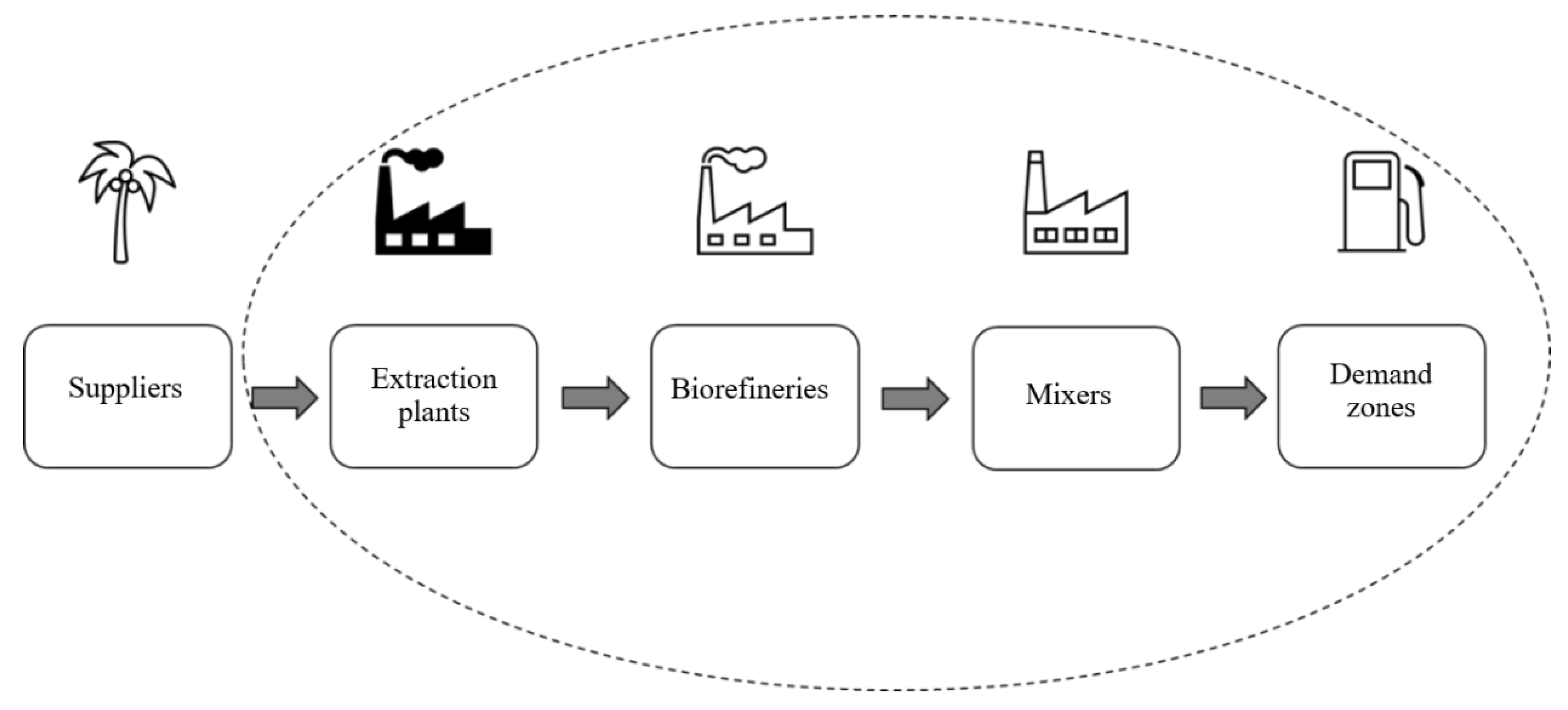
Figure 2.
Flow of the Warm-Start Procedure.
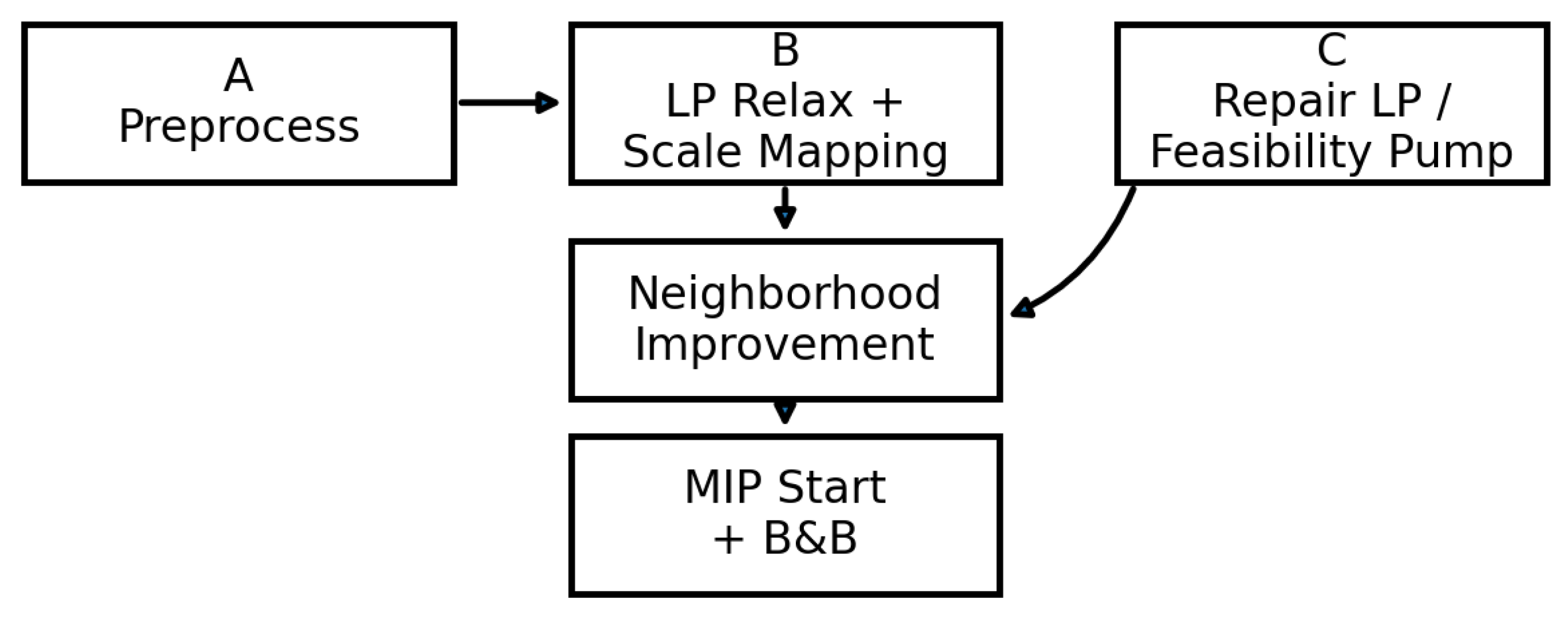
Figure 3.
Variation in profitability due to increases in revenues.
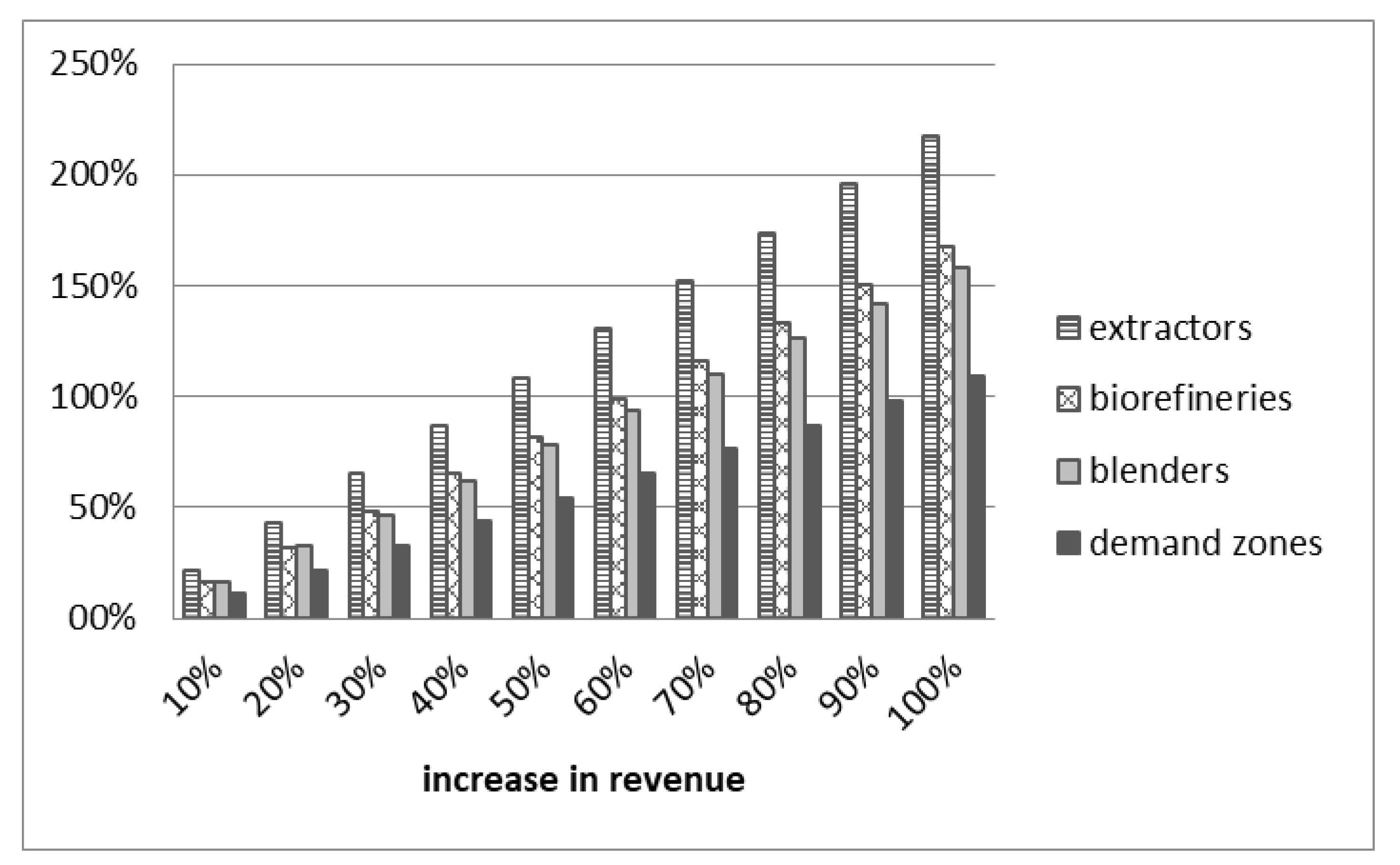
Figure 4.
Utility variation due to increases in facility capacities.
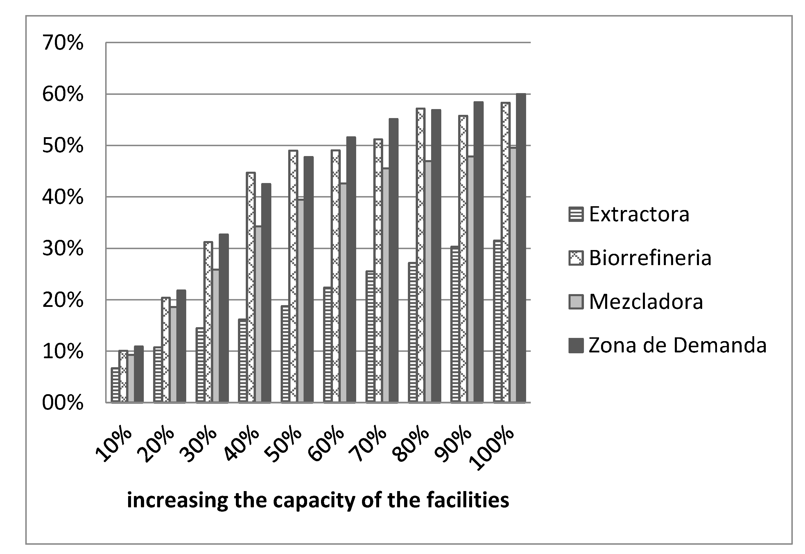
Table 2.
Comparative Analysis of Biodiesel Supply Chain Models.
| Reference | Model type | Supply chain scope | Objective | Novelty |
|---|---|---|---|---|
| Huang et al. [21] | MIP | Upstream + Mid-stream | Minimize cost | Includes seasonal supply modeling |
| Zhang et al. [30] | Simulation + LP | Downstream | Maximize service level | Real-time blending dynamics |
| Gutiérrez et al. [20] | Simulation + LP | Downstream | Maximize service level | Real-time blending dynamics |
| This study | MIP with VI | Midstream + Down-stream | Maximize net profit | Tactical integration with economies of scale |
Source: Authors’ own elaboration based on reviewed literature.
Table 4.
Supply chain network configuration.
| Instance 1 | Instance 2 | Instance 3 | Instance 4 | |
|---|---|---|---|---|
| Number of palm fruit suppliers i | 4 | 5 | 6 | 7 |
| Number of CPO extractors j | 5 | 6 | 6 | 7 |
| Number of diesel biorefineries q | 4 | 5 | 6 | 7 |
| Number of blenders k | 4 | 5 | 6 | 7 |
| Number of demand zones l | 3 | 4 | 5 | 6 |
| Number of scales in j | 2 | 3 | 3 | 3 |
| Number of scales in q | 2 | 3 | 3 | 3 |
| Number of scales in k | 2 | 3 | 3 | 3 |
| Number of items or products in i | 3 | 4 | 5 | 6 |
| Number of items or products in j | 3 | 4 | 5 | 6 |
| Number of items or products in q | 3 | 4 | 5 | 6 |
| Number of items or products in k | 3 | 4 | 5 | 6 |
| Number of items or products in l | 3 | 4 | 5 | 6 |
Table 5.
Value of the objective function and performance variables.
| Instance 1 | Instance 2 | Instance 3 | Instance 4 | |
|---|---|---|---|---|
| Objective function value | 1,227,762 | 1,558,010 | 1,182,420 | 1,301,439 |
| Total Variables | 814 | 2,272 | 3,823 | 6,273 |
| Binary Variables | 288 | 900 | 1,530 | 2,520 |
| Number of constraints (not including non-negativity constraints) | 1,376 | 3,405 | 5,689 | 17,704 |
| Memory used (KB) | 326 | 762 | 1,278 | 2,899 |
| LP Iterations | 15,692 | 860,866 | 21,359,983 | 47,366,532 |
| Nodes explored (×103) — Baseline: | 0.191 | 13.786 | 218.940 | 650.025 |
| Final MIP gap (%) — Baseline: | 0.00 | 0.00 | 0.00 | 0.00 |
| Seeded MIP start (Y/N) — Baseline: | N | N | N | N |
| Nodes explored (×103) — Warm start: | 0.150 | 9.650 | 157.600 | 487.500 |
| Final MIP gap (%) — Warm start: | 0.00 | 0.00 | 0.00 | 0.00 |
| SD (Warm start) | 0.010 | 0.450 | 7.500 | 20.000 |
| Seeded — Warm start (Y/N): | Y | Y | Y | Y |
| TTFF (s) - Baseline | 4 | 20 | 900 | 1,800 |
| TTFF (s) - Warm Start | 1 | 6 | 315 | 720 |
| TTFF - Reducción (%) | 75 | 70 | 65 | 60 |
| TTFF (s) - SD Warm Start * | 0.3 | 1.0 | 45 | 90 |
| CPU (s) - Baseline | 6 | 62 | 2,759 | 10,153 |
| CPU (s) - Warm Start | 5 | 50 | 2,200 | 8,000 |
| CPU - Reducción (%) | 16.7 | 19.4 | 20.2 | 21.2 |
| CPU (s) - SD Warm Start * | 5 | 7 | 45 | 80 |
* empirical SD across n = 10 independent runs per instance with distinct random seeds; no imputation was used. Confidence intervals are t-based.
Disclaimer/Publisher’s Note: The statements, opinions and data contained in all publications are solely those of the individual author(s) and contributor(s) and not of MDPI and/or the editor(s). MDPI and/or the editor(s) disclaim responsibility for any injury to people or property resulting from any ideas, methods, instructions or products referred to in the content. |
© 2025 by the authors. Licensee MDPI, Basel, Switzerland. This article is an open access article distributed under the terms and conditions of the Creative Commons Attribution (CC BY) license (http://creativecommons.org/licenses/by/4.0/).
Copyright: This open access article is published under a Creative Commons CC BY 4.0 license, which permit the free download, distribution, and reuse, provided that the author and preprint are cited in any reuse.


