
Submitted:
02 October 2025
Posted:
03 October 2025
You are already at the latest version
Abstract
The ability to predict the vapor pressure and vapor-phase composition of hydrocarbon mixtures (such as jet fuel or its un-refined precursors) and partially vaporized hydrocarbon mixtures is important to simulations of processes that involve vaporization. For example, models or simulations of distillations, flash point, chemical/combustion properties of the vapor phase of partially vaporized systems, and jet-engine ignition all benefit from a rudimentary model of vapor pressure given inputs of liquid-phase composition and temperature. One approach toward the rudimentary model is Raoult’s Law which is elegantly simple (\( p_i=x_i*P_(vap,i) \)) but inaccurate at low mole fraction (\( x_i \)). Another approach is to use a so-called activity coefficient (\( a_i \)) to more accurately represent the partial pressure of the ith component (\( p_i=a_i* x_i*P_(vap,i) \)) where the activity coefficient is estimated from an algebraically complex formula (e.g. the UNIFAC model) involving a plurality of combinations of mole fractions, molecular group fractions, Van der Waals volume and area as well all possible interaction terms between the groups. Invariably, the corrections based on activity coefficients involve an empirical fit to vapor pressure data that is sparsely (if at all) populated by mixtures that resemble fuel either in regard to the number of components or even the mole fraction of a given component. For example, the reference, “average” conventional jet fuel designated as “A-2” by the National Jet Fuel Combustion Program which has been leveraged by numerous research studies contains just 4.3%m n-nonane, its most populous component, while the simple mixtures used to anchor vapor pressure models such as UNIFAC are unlikely to have any component present at less than 10%mol. In addition to a lack of validation to naturally representative mole fractions, models such as UNIFAC can be computationally burdensome for simulations that require a very large number of vapor pressure and composition determinations. Here we present an alternative correction to Raoult’s law where the vapor pressure of the ith component is represented by a modified form of the Clausius-Clapeyron equation where the reference temperature (\( T_(ref) \)) is replaced by a simple algebraic function that converges to \( T_(ref) \) as \( x_i \) approaches 1 while smoothly increasing from this value as \( x_i \) decreases. Simultaneously, the heat of vaporization (\( ΔH_(vap,i) \)\( T \)) term is replaced by another simple algebraic expression that converges to \( ΔH_(vap,i) \) \( T \) as \( x_i \) approaches 1 while smoothly decreasing as \( x_i \) decreases. In this model, the temperature dependent heat of vaporization is tuned at each temperature such that the Clausius-Clapeyron equation reproduces the correct vapor pressure of the neat material while the parameterized algebraic corrections are tuned to vapor pressure data of mixtures involving n-pentane, toluene, and dodecane where the mole fraction of n-pentane and toluene are maintained below 10%mol. Validation of the resulting model is accomplished by comparing modeled vapor-liquid equilibrium systems with experimental measurements.
Keywords:
sustainable aviation fuel
; hydrocarbon mixtures
; vapor pressure
; vapor liquid equilibrium
1. Introduction
Volatility properties of jet fuels are known to have some impact on the safe operation of aircraft. As such, certain representative properties are specified in governing specifications such as ASTM D1655, DEF STAN 91-091, GOST 20227 or GB 6539. Flash point relates to aircraft-level fire safety. Initial boiling point relates to fuel pump cavitation and fuel control instabilities that could be caused by two-phase flow. The temperature at which 10% of petroleum-derived jet fuel (T10) has vaporized is correlated with engine ignition characteristics. During thermal soak-back after a jet engine is shut off, the vapor pressure inside the closed circuit from the fuel metering unit to the fuel nozzle valves could exceed the valve cracking pressure and lead to fuel burping into the fuel nozzles where it can bake until it turns to coke. A similar phenomenon can happen during part power operation during which some fuel circuits are turned off (called staging). The dry-out rate of passively purged, staged fuel circuits, similar to droplet evaporation rates depends on mass transfer rate, vapor pressure and liquid-phase surface area. Finally, the end point of the distillation is correlated with combustor coking and unburned hydrocarbon emissions. None of these relationships are one-to-one. Moreover, the above listing of operating concerns that could potentially be impacted by fuel properties is not exhaustive. Indeed, an exhaustive list of potential concerns is not generally known [1]. Motivated by such known and unknown factors, two volatility properties, (T50–T10) and (T90–T10), where the subscript refers to the volume fraction distilled, were added as “extended requirements” in the quality specification, ASTM D7566, governing aviation turbine fuels containing synthesized hydrocarbons.
Specifically, the rate of evaporation across a plurality of temperature, convective, and dwell time conditions is directly related to potential operating concerns. Unlike Tn, the vapor pressure (Pvap) of fuel droplets or sheets is directly proportional to their evaporation rate at all operating conditions. The importance of this is recognized by the community and as such the vapor pressure as a function of temperature is listed as a tier 2 property in ASTM D4054, “Standard Practice for Evaluation of New Aviation Turbine Fuels and Fuel Additives”. While maintaining an approximate match to a family of Pvap vs. temperature curves derived from a representative survey of petroleum-derived jet fuels is a prudent goal for developers of sustainable aviation fuel (SAF) or other fuels with synthetic components, it is neither sufficient nor necessary in all circumstances.
The chemical (and to a lesser extent, the transport) properties of fuel vapor varies throughout the evaporation time scale and so do the volatility properties of the liquid that has yet to evaporate. Chemical properties, represented by derived cetane number, radical index, threshold sooting index, etc. play an important role in lean blowout, particulate matter (nvPM) emissions, and the rate of heat release during combustion—indicating potential impact on combustion dynamics, combustor temperature distribution and combustion efficiency, for example. The composition of the remaining liquid, in tandem with the temperature at its interface with air determine its vapor pressure and hence its evaporation rate for the relevant transport conditions. All these variances are hereafter referred to as preferential evaporation in this article.
Property models that neglect to track changes in liquid-phase composition throughout the evaporation time scale sacrifice the capability to directly capture the impact of preferential evaporation. However, through correlation with specific points on the ASTM D86 distillation curve, some indirect capturing of preferential evaporation may occur provided the relative population distribution of each type of hydrocarbon in the boiling sample is similar to the database of fuel samples from which the model was built. Mendes et al. [2] published a regression model to predict the Reid vapor pressure (Pvap @37.8 °C) of conventional gasoline based on its ASTM D86 distillation curve. Two groups [3,4] published separate regression models built from Raman spectrographic data to predict Reid vapor pressure and octane numbers of petroleum fuels. Flumignan et al. [5] built a regression model built from chromatographic data to predict density, distillation curve and octane numbers of Brazilian gasoline, while Cocco et al. [6] used chromatographic data of 25 samples to build an artificial neural network model to predict density, distillation curve and Reid vapor pressure of Brazilian gasoline. It is unknown whether any of these models capture the impact of preferential evaporation, even for petroleum-derived gasoline, or whether any are valid for jet fuel range hydrocarbons.
Other notable examples of simulated, D86 distillation curves include ASTM D2887 (which employs chromatographic data) and the work of Mondragon et al. [7] (which employs thermogravimetric data). The intense interest around this task is a testimonial to its value, which appears to be rooted in the reduction of sample volume required to determine properties that are controlled by some quality specification. Not only do such models neglect to directly capture the impact of preferential vaporization, but they offer little value to efforts, such as those described by Miller et al. [8], to maximize biomass in SAF by optimal selection of distillation fraction or other refinement processes of the synthetic blend component. Furthermore, such models, barring a simulation of the base data, do still necessitate some mass of representative sample to get the input data.
Within the so-called, tier- suite of property models published by Yang et al. [9], vapor pressure is calculated by Dalton’s Law with partial pressured calculated by Raoult’s Law, and simulated D86 distillation is carried out by incremental mass extraction per the composition of the simulated vapor phase. Miller et al. [8] now execute simulated distillation using this same approach and have observed significant error in the prediction of T90. Such error could stem from distillation assumptions (e.g., number of theoretical plates), inaccurate composition input, or propagated errors in components’ vapor pressures.
In a provocative article published in 1995, Hawkes [10] proclaimed that Raoult’s Law is deceptive, which is somewhat interesting in that Wilson’s model of activity coefficients was introduced in 1964 [11] and it was already common by then, in some circles, to use activity coefficients to scale the partial pressures that are predicted by Raoult’s Law to arrive at a more accurate description of the vapor-liquid phase equilibrium. By 1975, the unsettling fact that vapor-liquid equilibrium data was needed to determine one or more of the parameters used in the Wilson model (and several of its off-shoots) was addressed by Fredenslund et al. [12] by relating these terms to groups (e.g., >C<, -CH3, aromatic CH, etc.) that are contained in all molecules where the contributions from each group were determined by fitting to vapor-liquid equilibrium data for a variety of binary mixtures, which in theory would permanently establish these contributions so they could be used without modification for other molecules and mixtures which were not part of the original database. This model is called the UNIFAC model and is included in publicly available software such as Aspen Plus, DWSIM, and ChemCAD. Yet more fundamental models based on intermolecular potentials (RGEMC) [13] or simulated osmotic pressure (OMD) [14] are available in molecular dynamics software such as LAMMPS.
Here, our goal is to evaluate simpler corrections to Raoult’s Law as fuels are comprised of thousands of different molecules and simulated fuel distillations may require several thousand determinations of the vapor-liquid equilibrium. Among these thousands of molecules only seven carbon types are significantly represented; four aliphatic carbon types (-CH3, -CH2-, >CH- and >C<) and three aromatic carbon types (protonated aromatic carbon, substituted aromatic carbon and bridgehead aromatic carbon). Within UNIFAC, four terms are used to represent the four aliphatic carbon types and two terms are used to represent aromatic carbon; protonated or not protonated. In contrast, we are not distinguishing between carbon types or molecular structure. Rather, we acknowledge that every molecule is forced into an environment determined by the liquid mixture Gibbs energy minima which differs significantly from that of pure liquids, which is the root cause of a non-zero heat of mixing. While the magnitude of the heat of mixing is ~500 times less than the magnitude of the heat of vaporization, we postulate that enthalpy difference can have a significant impact on the vapor pressure of each liquid-mixture component. The main effect on the heat of mixing of jet-fuel range hydrocarbons is mole fraction, not molecular structure, so here we develop a model framework that is based exclusively on mole fractions as input and a tuning database of binary mixture vapor pressures where the (much) more volatile component is present at mole fractions ranging from 0.01 to 0.09. Over this range of mole fractions, the traditional, activity-coefficients, approach to correcting Raoult’s Law is not validated to the best of the authors knowledge.
The approach we consider is described in the Theory section of this article, which directly follows this paragraph. Then, we describe the materials, test conditions and testing methodology used to support determination of the adjustable parameters of this modeling approach and this is followed by the Results Section where the empirically-based correction is derived. Validation of the resulting model is accomplished by comparing modeled vapor-liquid equilibrium systems with experimental measurements. Finally, a summary of the major findings of this study is presented in the Conclusion Section.
2. Theory
The earliest model of vapor pressure can be traced back to Clapeyron [15] nearly 190 years ago. Since then, many model refinements have been published, starting with Clausius [16] who published the form that is found in many current physical or general chemistry textbooks. These models relate the vapor pressure of a liquid to its latent heat of vaporization () and imply that equals the slope of verses inverse temperature . Interestingly, the general form of this model can also be derived from kinetic theory although it was originally conceived entirely from fundamental principles of thermodynamics. In 1884, Trouton [17] shared a recognition that the entropy of vaporization at ambient pressure of most liquids is approximately the same, 87.3 J.K−1.mol−1 which implies that is directly proportional to the normal boiling point.
By definition, the vapor pressure of a substance is the pressure at which the rate of adsorption of gaseous molecules that strike the surface of a liquid equals the rate of desorption of molecules from the surface of that liquid. The evaporation rate is the difference between the rate of desorption and the rate of adsorption and goes to zero at equilibrium. Theoretically, the rate of desorption of any component in a liquid mixture could be limited by the diffusion of volatile molecules to the surface or by the fundamental process of desorption.
As accommodated by Antoine’s [18] semiempirical correction to the vapor pressure model, published 1888, the activation energies of whatever steps control the rate of desorption in pure materials are not generally equal to as, by definition, is the enthalpy difference between the liquid and gaseous phases of the material. The activation energy is coincidentally nearly equal to in many systems. However, the desorption process could occur in multiple steps and the activation energy governing the rate of each step is, more likely than not, greater than the energy difference between the two geometrical configurations that define the step. In other words, even for pure materials, the slope of verses inverse temperature could be higher or lower than .
As recognized by Antoine [18] and many authors since then [19], the is not exactly linear with , which suggests that the rate limiting steps in the desorption process are influenced by the bulk change in molar volume as temperature varies. In other words, it matters how many 1st or 2nd nearest neighbors to a desorbing molecule are vacant. By extension, it should also matter how many 1st or 2nd nearest neighbors are heterogeneous molecules. To estimate the order of magnitude of this effect, we compare the heat of mixing, which is approximately 25 J/mol [20] for jet fuel range hydrocarbons, to the heat of vaporization of a representative fuel molecule, n-dodecane, which is 44,000 J/mol. While the heat of mixing has a small (<0.1%) impact on the heat of vaporization, its impact on the desorption rate is approximately 0.6% at the normal boiling temperature of n-dodecane. Intuitively, this impact increases as mole fraction decreases because molecules of this mixture component are progressively less likely to have homogeneous neighbors as mole fraction decreases.
Raoult’s Law, in combination with a somewhat modified version of the Clausius-Clapeyron equation, is reproduced here as equation 1, where is mole fraction, is 1 atmosphere, is the normal boiling point of pure component i, and the remaining term is expanded below. The activation energy () varies with temperature and the actual vapor pressure of pure component, i according to equation 2, such that equation 1 returns a correct vapor pressure at all temperatures, within the range of the data, when the mole fraction is unity. Pragmatically, an Antoine equation or a Wagner equation [21] is used to represent discrete () data points continuously, for each pure component. A spline is used to represent over the range of temperature ±5 °C from the normal boiling point.
The reason why equation 1 fails to accurately represent the actual partial pressure of component, i in the vapor phase () is not just because varies as the identity of nearest neighbors change but also because the reference temperature (, the temperature at which atm) varies as the effective surface area of the ith component, its concentration, varies. In other words, both () and () are concentration dependent but the conventional approach to remediate the failure of Raoult’s Law is to maintain each of these terms as constant and instead scale the resulting partial pressure by an activity coefficient which depends, not only on the identity of the ith component, but also on its concentration, the temperature of the system and the identity and concentration of every other component in the mixture. Here, we evaluate simpler ways to make this correction.
2.1. Data Reduction Strategy
We consider replacing () and/or either or both occurrences of () in Equation (1) with a simple, parameterized function of mole fraction, the exact form of which is to be determined, for the purpose of minimizing the root mean square error (RMSE) of the predicted vapor pressure relative to the measured vapor pressure. These variants of equation 1 are expressed here as Equations (1A)–(1D). Ultimately, one (or none) of these equations will be recommended for vapor pressure, evaporation rate, and distillation simulation of complex fuels. For comparison, the activity coefficient approach, is represented by the UNIFAC model which is described in the next sub-section.
In these equations, and are scaled reference temperatures, while is a scaled activation energy. Two functional forms of the scale factor were tried for each term, where is adjusted to minimize the RMSE. The trial 1 scale factor provided a lower RMSE in every case.
- or
- or
The same value of applies to all three components; n-pentane, toluene and n-dodecane, as well as (conceptually) every component in jet fuel. A different value of was determined for each model; 1A, 1B, 1C, and 1D. For model 1D, two separate tuning parameters were derived, one for and one for , and not surprisingly this model provided the lowest RMSE of the set. Relative to the UNIFAC modeling scheme, this modeling approach sacrifices dependencies on component identity (differences in interaction energies, molecular shape and size) in favor of simplicity and generality. It also potentially gains an ability to elegantly capture some of the composition-specific temperature dependencies through its linkage to the Clausius-Clapeyron equation and the best available, temperature-dependent component data.
2.2. Reference Model (UNIFAC) Description
The UNIFAC model is described in detail by Fredenslund et al. [12] and is one of several derivatives of earlier models of activity coefficients. In this model, the activity coefficient of component, i is assumed to be a product of two terms: the combinatorial term and the residual term.
The log of the combinatorial term is then estimated by a sum of four more terms, involving six different terms; one of which is the mole fraction of component, i, and one is a modelling constant set equal to 10. The four remaining terms are different arithmetic combinations of mole fractions, van der Waals volumes, and van der Waals surface areas of every component in the mixture.
The log of the residual term is the sum over all groups (-CH3, etc) in the mixture, of the difference between two new terms where one of these relates to the group’s contribution in the mixture and the other relates to the group’s contribution in pure component, i. The same expression is used to define each of the ‘new’ terms. The independent paraments in this expression include the van der Waals surface area of each group as well as group fraction (analogous to mole fraction), and it involves a group interaction parameter. A large set of group interaction parameters were determined by Fredenslund et al. [12] by a non-linear, least squares data reduction scheme where vapor-liquid (and liquid-liquid) equilibrium data of binary systems from 200 different sources were used as the foundational data base.
The molecules used in this work are comprised of four groups: -CH3, -CH2-, arCH and arC-CH3. The methyl group of toluene is combined with the aromatic carbon that it is bound to and this pair is treated as one group. All four of these groups contribute uniquely to the van der Waals volume and surface area calculations, but for the purpose of interaction parameters, the methyl and ethyl groups are considered identical. However, the interaction terms () are not symmetric so , meaning we have to consider six interaction terms rather than three. A compilation of the values used in this work is provided in Table 1. The spreadsheet used to compile all of the arithmetic combinations of these parameters is provided in the Supplemental Material, entitled, “UNIFAC Vapor Pressures”.
3. Methods and Materials
3.1. Vapor Pressure Measurement
The Eravap device, manufactured by Eralytics, was used to measure vapor pressure of liquid samples. The device employs factory-installed software to control sample volume, fill temperature and sample temperature as per user-selected test methodology. We considered the ASTM D6378, triple point expansion method as well as the Eralytics, lowVP module. For both methods, sample is pulled into the measuring cell (see Figure 1) via an actuated piston. A pre-set number of rinse cycles are used to saturate the gas in the measuring cell with sample vapor. Upon conclusion of this conditioning operation, the piston is positioned to a depth corresponding to a chamber volume equal to 4 mL. The suction created by moving the piston up to a depth corresponding to 5 mL is responsible for pulling 1 mL of liquid sample into the measuring cell. During the filling process, sensed pressure is monitored to flag potential filling error. Once the sensed pressure is found to be within 5 kPa of the (air-only) ambient pressure, which was recorded prior to rinsing, a second timer (t2) is activated and the first timer (t1) is stopped. The first timer started upon opening the inlet valve (see Figure 1) to the sample. In the controller module called ASTM D6378, the inlet valve is closed when t2 = t1/3.
The ASTM D6378 module employs four pre-set volumes (the smallest being 4 mL), which are created by moving the piston within the sealed measuring cell (see Figure 1). The slope of PV vs V at constant T is the vapor pressure of the sample at that temperature. The total number of moles as well as the number of sample moles are determined from the ideal gas law, using total pressure and vapor pressure, respectively as inputs. The number of moles of air is the difference between these two determined quantities. The Eralytics, low VP module differs from the ASTM D6378 module in several ways. Notable differences include longer fill times achieved by decreasing the pressure variation from ±5 kPa to a lower value (~±0.15 kPa), implementing a degassing procedure to rid the liquid phase of any trapped bubbles, and executing a triple expansion at a temperature higher than the test temperature to determine the number of moles of air in the sealed measuring cell. For further description of this method, readers are referred to the Eralytics User Manual for the Eravap device.
For three pure solvents, n-pentane, toluene and n-decane the indicated vapor pressure as a function of temperature was compared to reference data published by NIST [22]. When using the ASTM D6378 module, we found discrepancies ±1.5 kPa, which is much higher than desired for this work. For this reason, we selected the Eralytics lowVP module for all vapor pressure determinations reported here. According to Eralytics, this method has a repeatability of ±0.15 kPa for all samples at temperature between −20 °C and 120 °C with a vapor pressure between 1.0 kPa and 1000 kPa. Our observations are consistent with the quoted repeatability value.
3.2. Materials
The solvents listed in Table 2 were used to make a variety of mixtures containing 0–10% mol of light components. The heaviest component (n-dodecane or n-tetradecane) used in 2- or 3-component mixtures was present at higher concentration.
Binary mixtures of n-pentane or toluene in n-dodecane, each at 4 different blending ratios and heated to 70 or 100 °C were used to determine the tuning parameter(s), . Both sets of binary mixtures included 0.04, 0.06 and 0.09 mole fraction of the lighter component, while the n-pentane/n-dodecane set also included one mixture with 0.02 mole fraction of n-pentane and the toluene/n-dodecane set also included one mixture with 0.06 mole fraction of toluene. A large difference in volatility was deliberately chosen to minimize the impact of errors stemming from the vapor-liquid equilibrium of the solvent; focusing instead on a single volatile component at low mole fraction. For example, the liquid mixture containing 0.04 mole fraction toluene produces a vapor at 100 °C that consists of at least 60% toluene with wide variation depending on which model is used to predict the component vapor pressures.
Ternary mixtures of n-pentane, toluene and n-dodecane were used as a first level of model validation. In these mixtures the mole fractions of toluene and n-pentane were made equal to each other: 0.01, 0.04, 0.07 and 0.09. At minimum, the model developed in this work should predict the vapor pressure of these mixtures at 70 and 100 °C more accurately than any of the general models regardless of its relative simplicity because its parameters were trained specifically on n-pentane and toluene data. Extension of this model to higher temperatures, corresponding to the ambient-pressure bubble points is somewhat more stressful but each of the models considered in detail here employ the same vapor pressure curves of the pure components so even here, the model developed in this work should be more accurate than Raoult’s Law and the correction to it based on UNIFAC-determined activity coefficients.
Ternary mixtures; (cyclohexane, o-xylene, n-tetradecane) and (isooctane, o-xylene, n-tetradecane) were used to evaluate the generality of the model. In one experiment, the pot temperature of a mixture made from 2.55 g of cyclohexane, 2.56 g of o-xylene and 44.99 grams of n-tetradecane was compared with modelled liquid temperature of a system for which 0 or 1.0 %vol of the liquid is assumed to have vaporized, but present in the reflux apparatus (Figure 2) above the surface of the boiling liquid and below the condenser. In another experiment, 100 mL of a mixture made from A: (10.36 g of cyclohexane, 10.04 g of o-xylene and 90.93 grams of n-tetradecane) or B (10.02 g of isooctane, 10.01 g of o-xylene and 79.96 grams of n-tetradecane) was distilled according the method described as ASTM D86. A brief description of this experiment is provided in this section under the “distillations” heading.
Finally, data was extracted from the work of Hung et al. [24]. Although none of the ninety (T, P) vapor–liquid equilibrium points they measured satisfy our predetermined filter criteria, the dataset serves as a valuable benchmark for assessing how our model performs when applied to systems clearly outside the training set’s range. For the record, our predetermined filter criteria were: non-associated components, <0.10 mole fraction of the volatile component(s) which we call solute, >100 K difference between the solute and solvent normal boiling points, and mixture vapor pressure between 1.5–101.3 kPa. Their study involved five sets of binary mixtures involving n-nonane, n-octane, methylcyclohexane and methylcyclopentane and three fixed temperatures (120, 160, 200 °C). We selected the points at 120 °C to minimize the confounding effects of real gas behavior. Three older datasets by different authors were also evaluated but the data contained in those reports, relative to Raoult’s Law predictions showed deviations much different from our observations leading us to question whether we properly understand the experiment they conducted.
3.3. Reflux Experiment
The glassware shown in Figure 2 was used to measure the liquid temperature of a boiling mixture. Fifty milliliters of a cyclohexane/o-xylene/tetradecane mixture was inserted into the 100-mL round-bottom flask and heated until a steady-state reflux was established. Ordinary tap water was used as the coolant; fed through the condenser sleeve from the bottom port up, through the top port. Negligible pot temperature (lower thermocouple) variation was observed as the heat flux (vigorousness of the boil) varied. However, the condensate temperature (upper thermocouple) varied significantly with heat flux and with subtle changes in its vertical position. For this reason, the upper thermocouple temperature is not reported here, although it was used to verify internal coherence. For the purpose of comparing the measured liquid (pot) temperature with the theoretical bubble point of the liquid mixture, the dynamic hold-up was approximated to contain the equivalent of 1 %vol of the sample; 0.5 mL at reference (lab) temperature. The theoretical temperature corresponding to 1 %v distilled was compared with the measured pot temperature. Additionally, the measured temperature corresponding to the first visual observation of bubbles was recorded as well as the bubble point as predicted by the vapor pressure model. In this way, there is a band represented for both the measured and modeled temperatures.
3.4. Distillations
Distillations were carried out with the apparatus shown in Figure 3, achieving a collection rate of 1.5–3.0 mL/min from 5% distilled to 50% distilled, which is lower than the requirement stated in ASTM D86 (4–5 mL/min). The vertical placement of the thermocouple junction is controlled by its sub-assembly which inserts into the ground-glass fitting at the top of the column. Its depth was determined from prior work, manually tuned to reproduce the distillation curve determined with a commercial apparatus conforming fully to the specifications of ASTM D86. The condenser arm is water-cooled and the collection cylinder is bathed in quiescent air at ambient temperature and pressure. The only vent in the distillation apparatus is at the exit of the condenser arm. Heat is applied via an electrically controlled hot-plate to the bottom of a 125-mL, round-bottom flask which is filled initially with 100 mL of sample. The dimensions of the distillation column, condenser, and collection cylinder (100 mL, graduated) are similar to those of the corresponding pieces as specified in ASTM D86. No fractionating media is present in the column.
The volume of dynamic holdup (which includes all mass, liquid or vapor, that is not present as liquid in the pot or collection cylinder) varies with the temperature gradient [25] between the bubble point of the liquid phase (in the pot) and the dew point of the vapor phase at the inflection point in the condenser arm as well at the heat flux applied to the bottom of the round-bottom flask. By adjusting the heating rate periodically to maintain a distillate collection rate of 1.5–3.0 mL/min, the variation in dynamic holdup throughout the course of the distillation is reduced. The dynamic holdup volume is the largest source of mismatch between the recorded distillation curve temperatures (Tn) and the actual distillate temperature throughout a distillation. It can be anywhere from 0.5 to 10 mL depending on sample composition [25], but is more commonly ~2.6 mL.
Larger dynamic holdup volumes suggest a higher degree of fractionation because liquid that forms upstream of the inflection point on the condenser arm will drain toward the heat and re-vaporize (whether fully or partially) prior to blending back into the pot. Bounding assumptions of one or two theoretical plates of separation are assumed here for the purpose of comparing modelled distillations with measured distillation curves and distillate compositions. The theoretically-estimated temperatures should be consistently higher than the measured temperatures (Tn) if they accurately reflect the actual temperature of a system with n %v ‘not-in-pot’, which includes dynamic holdup volume and collection volume, instead of n %v collected.
The fraction distilled is defined as the volume of distillate collected divided by the volume of sample charge, which is 100 mL. The temperature can be monitored throughout the distillation, although usually the operator will only record the temperature at pre-determined distillate volumes. For example, at 10 %V distilled, the operator may record T10 if 10 %V is a pre-determined test point. In this work, the operator has recorded four points for distillation of the ternary mixture (T5, T10, T15, and T20). Specific to this work, a 0.2 mL sample of distillate was pipetted from the collection cylinder at each of the scheduled test points for the purpose of characterizing its composition via GCxGC/FID. The composition of distillate is not subject to error introduced by the dynamic holdup. To minimize distillate sample inhomogeneity, the material in the graduated cylinder was swirled and agitated by pulsing with five pipette volumes prior to each collection, and to minimize the risk of evaporative loss from the sample it was immediately transferred to the gas chromatograph. The sampled volumes were not compensated for later collections, meaning the actual collected distillate volume at the second test point, for example, was 0.2 mL greater than indicated by the test point schedule, which consistently referenced the volume of material in the graduated cylinder.
3.5. Distillate Composition Analyses
The composition of each distillate was determined by two-dimensional gas chromatography with an in-series flame ionization detector (FID) according the method described originally by Striebich and Shafer [26] and later by Heyne et al. [27] In these experiments, the composition determination was particularly simple because the samples were made of just three highly pure components, that eluted over easily distinguished time/time domains.
One micro-liter of undiluted sample was injected into the head of the gas chromatograph. The integrated FID response corresponds to the mass of each component that elutes over the user-defined, time domain of the integration. Since all masses are determined, and the identity of all species are known in advance, the corresponding mass, mole, or volume fractions of each component can be readily determined.
3.6. Modeled Distillation
Idealized 1-plate and 2-plate distillations were completed for each experimentally distilled mixture and each vapor pressure model (this work and Raoult’s Law). The initial condition is 100 mL of test mixture of known composition at ambient temperature and pressure (Pamb), from which total moles is determined. This mixture heated (or cooled) in increments of 0.001 K until its vapor pressure reaches (Pamb ± 0.001) kPa. At that point, for 1-plate distillations, 0.1 %mol of material having composition determined by the modeled vapor phase is removed from the system. The dew point of this drop is determined by cooling (or heating) the vapor in increments of 0.001 K until a liquid of that composition produces a vapor pressure of (Pamb ± 0.001) kPa. For 2-plate distillations, two vapor phase compositions are tracked. The first one (the higher-temperature one) is determined by the temperature and composition of material in the pot, the second one (the lower-temperature one) is determined by the temperature and composition of the first drop. The second bubble point temperature is equal to the first dew point temperature. This temperature, along with the composition of the first drop (as well as the first vapor phase), determines the composition of the second phase. At this point, for 2-plate distillations, 0.1 %mol of material having composition determined by the second modeled vapor phase is removed from the system. The dew point of this (second) drop is determined by cooling (or heating) the vapor in increments of 0.001 K until a liquid of that composition produces a vapor pressure of (Pamb ± 0.001) kPa. In each case the modeled (final) dew point is compared with experimentally measured condensate temperatures.
To model a significant span of the distillation curve, this process repeats up to 1000 steps; with incremental reduction of liquid in the pot at each step. To avoid numerical issues that are likely to arise somewhere (between 950 and 1000 steps) as the quantity of material being extracted becomes significant relative to the total material left in the system, we stopped the numerical distillations at 950 steps. The (first) bubble point temperature, (final) dew point temperature and composition of the extracted drop is recorded at each step. The fully-mixed distillate composition is also updated at each step.
4. Results
4.1. Tuning Vapor Pressure Models
The mixtures of n-pentane in n-dodecane and toluene in n-dodecane were used to represent the vapor pressure of an aliphatic or aromatic solute dissolved in a hydrocarbon solvent. A large volatility difference between the solute and solvent was chosen so that the composition of the vapor phase would be predominantly one component, the solute, even as the solute mole fraction in the liquid phase was taken down to 0.02 (n-pentane) or 0.04 (toluene). Thus, the confounding impact of solvent vapor pressure was minimized. Table 3 documents the normal boiling points and the Antoine coefficients for each of these three materials, where the Antoine equation was used to get the values of that were used in Equation 2. The singularity (in Equation (2)) that occurs when the temperature equals the normal boiling point does not arise at the tuning stage of this work because only test temperatures (70 and 100 °C) not equal to the normal boiling point of any of components were selected. Two values of temperature were chosen, effectively decoupling variation in from normal boiling point variation. A mix of aliphatic and aromatic hydrocarbons (one each) was deliberately selected because the entropy of vaporization, which effectively relates the normal boiling point temperature and the heat of vaporization, is somewhat different for each; approximately 86 J/mol/K and 73 J/mol/K for alkanes and aromatics respectively. Our intent here is to model each in the same way and to assess the error introduced by neglecting this difference.
For the n-pentane/n-dodecane mixtures vapor pressure data was recorded for mixtures with 2, 4, 6, and 9 %mol n-pentane at 70 and 100 °C. For the toluene/n-dodecane mixtures vapor pressure data was recorded for mixtures with 4, 6, 8, and 9 %mol toluene at 70 and 100 °C. These 16 data points were used to train the models. Figure 4 displays the best fit for each of the models defined in equations 1A-1D. The toluene/n-dodecane data are confined to panel a) and the n-pentane/n-dodecane data are confined to panel b). The motivation for showing all of these fits is to underscore the improvement offered by the second tuning parameter. For model 1D, the root mean square and mean absolute errors are 0.35 and 0.25 kPa respectively; substantially better than any of the single-parameter models. More importantly, for model 1D, the error is split evenly between each of the four groupings of data resulting in a mean error of just 0.09 kPa. In contrast, the errors of the single-parameter models are heavily skewed toward the toluene/n-dodecane mixtures while a temperature dependent pattern is also apparent. The tuned values of s, applicable to model 1D are reported in Equations (3) and (4).
C(xi) = Tref,i0 (1.0154 − 0.0154 ∗ xi)
B(xi)= Ea,i0 (0.77275 + 0.22725 ∗ xi)
A comparison of model 1D with other global models, UNIFAC and Raoult, is displayed in Figure 5. Surprisingly to these authors, the zero-parameter, Raoult’s Law misrepresents the n-pentane/n-dodecane vapor pressures at 100 °C by a whopping 22–60% while it essentially matches the toluene/n-dodecane vapor pressures at 100 °C. Compared with the 100 °C data, at 70 °C, the Raoult’s Law predictions decrease relative to the data for both sets of mixtures, which is a characteristic shared by the UNIFAC model predictions. The “corrections” to Raoult’s Law offered by the UNIFAC activity coefficients scale the vapor pressures of the toluene/n-dodecane mixtures (activity coefficients > 1) to higher values, which drives it in the wrong direction at 100 °C and the right direction at 70 °C. For the n-pentane/n-dodecane mixtures the UNIFAC model (activity coefficients < 1) scales the Raoult’s Law vapor pressures to lower values, which is closer to the data at both 70 and 100 °C, but still wrong by up to 31% at 100 C for the mixture containing 9.0%mol n-heptane. Clearly, the two-parameter model developed here shows greater promise than the activity coefficient approach represented here by the UNIFAC model which has a total of seven tuned parameters that are applicable to these mixtures.
4.2. Modeled Vapor Pressure Validation
The first level of validation to be discussed is to compare predictions to measurements of systems at slightly different conditions compared with the tuning dataset. Here we use ternary mixtures of n-pentane, toluene, and n-dodecane. For convenience of reporting the mole faction of toluene and n-pentane were prepared equal to each other. According to Raoult’s Law and model 1D the vapor pressure of this mixture should be essentially the sum of the vapor pressures of the respective binary mixtures because these models do not consider potential differences between components of differing identities and the slight reduction in n-dodecane’s contribution to the total vapor pressure is small because its vapor pressure is much lower than those of n-pentane and toluene. In contrast, the activity coefficients of the UNIFAC model are impacted by the identities of the other components. For example, at 9%mol, the activity coefficient of n-pentane is 0.811 at 70 °C for the binary mixture and 0.837 for the ternary mixture. Very astute readers may be able to see the effect of this difference by comparing Figure 5 and Figure 6 as the UNIFAC model is slightly more wrong for the ternary mixture than the binary mixture at this temperature even though it gets the vapor pressure of toluene right at this temperature. Comparison to the equation of state model [28] (EOS) used in REFPROP [29] which lacks key features relevant to complex mixtures such a fuels, reveals several notable observations. Although exaggerated relative to the measured vapor pressure curves, the EOS model predicts some curvature to the vapor pressure as a function of mole fraction, whereas this characteristic of model 1D (clearly present based on Equations 3 and 4) is not visibly apparent on the viewing scales of Figure 4, Figure 5 and Figure 6. The temperature dependence of the EOS model brings it closer to the measured values at 100 °C than at 70 °C which may not be surprising because the critical temperature is a focal point within that model’s framework. Most surprising to the authors however, was the magnitude of the errors afforded by this model in spite of its complexity and specificity to these three materials.
The next level of validation is to introduce a greater variety of materials and temperatures, resulting in vapor pressure up to ambient pressure. One simple way to get this data is to measure the temperature of a refluxing mixture. The temperature of the liquid phase is easy to get right and the pressure is the barometric pressure of the lab, but the composition of the liquid phase is somewhat confounded because some mass of sample exists as dynamic hold-up; vapor or condensed vapor that has not yet fallen back into the pot. In Figure 7, we show the measured reflux temperature of a mixture of o-xylene (8.6%mol), cyclohexane (10.8%mol), and tetradecane (80.6%mol) in comparison with the predicted bubble point resulting from model 1D, Raoult’s Law and the UNIFAC model. To account for the uncertainty of the liquid-phase composition, predictions corresponding to 0 and 1%vol are reported. The measured temperatures correspond to the moment when the first bubble was observed (bottom) and the moment it reached a steady-state temperature (top). For each of the models, the term in Equation (2) was represented by an Antoine equation with coefficients as documented in Table 3. As is quite evident from Figure 7, model 1D predicts a normal boiling point and refluxing temperature in far better agreement with the measured values than Raoult’s Law or the UNIFAC model. The liquid phase composition of 1%vol distilled for both model 1D and UNIFAC reflux temperatures (upper) was based on model 1D, and 1 theoretical plate was assumed since no removal of material is occurring in this system.
4.3. Literature Data
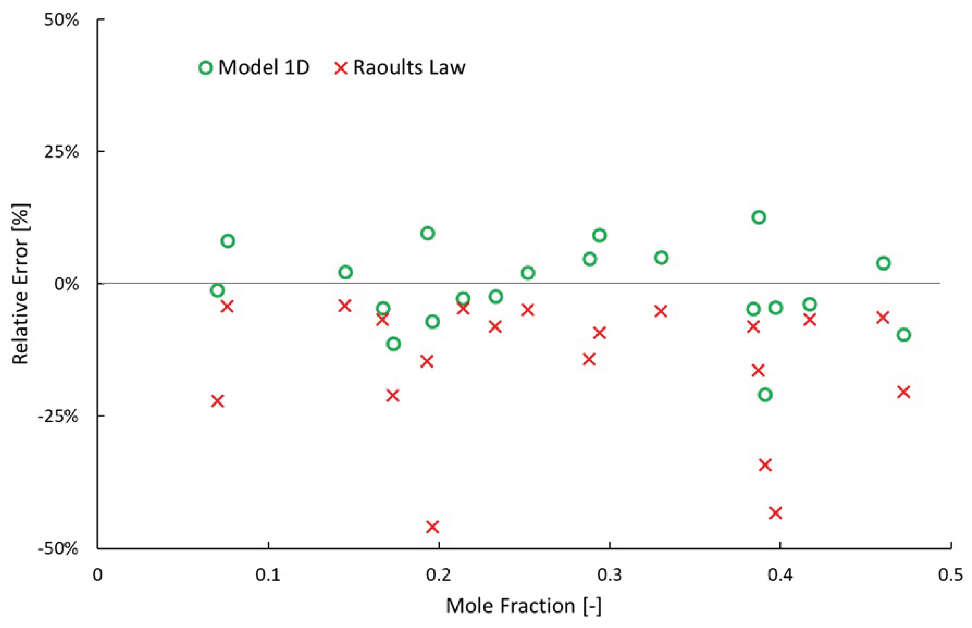
Recently, Hung et al. measured and predicted the vapor pressure of 20 different binary mixtures involving n-nonane, n-octane, methylcyclohexane or methylcyclopentane at 120, 160 or 200 °C. Their predictions were made via Aspen Plus V11 using COSMO-SAC, UNIFAC-DMD and two additional models with coefficients of binary interactions re-tuned to their measurements and Hayden-O’Connell fugacity coefficients. A description of the UNIFAC-DMD model (highlighting modifications to UNIFAC) is provided by Gmehling et al. [30] while a description of the COSMO-SAC model is provided by Hsieh et al. [31]. The mean absolute relative error (MARE) of UNIFAC-DMD and COSM0-SAC was 1.5% and 5.1% respectively. Comparatively, the simple 2-parameter model presented here results in a MARE of 5.1% and mean relative error (MRE), or over-prediction, of -0.7% considering only the data at 120 °C to avoid having to account for real gas differences relative an ideal gas. Model 1D overpredicts the vapor pressure of 11 mixtures while underpredicting the vapor pressure of 9 mixtures. In contrast, Raoult’s Law over-predicts the vapor pressure of all 20 mixtures; two of them by more than 40%.
Figure 8.
Relative Error of Vapor Pressure Predictions of Assorted Binary Mixtures of n-Nonane, n-Octane, Methylcyclohexane or Methylcyclopentane. The measurements were taken from the vapor-liquid equilibrium work by Hung et al. [24]. Temperature equals 120 °C and pressure equals 45.9–261.1 kPa. Relative error is defined as (measurement—prediction) divided by measurement.
4.4. Modeled Distillation Validation
The final validation of the vapor pressure model compares predicted distillation curves with measured distillation curves. However, the model of the distillation process may be more important to these curves than the vapor pressure model. Figure 9 is used to compare the measured distillation curve of the ternary blend containing initially 18.2%mol (9.3%vol) cyclohexane and 14.0%mol (7.8%vol) o-xylene with the balance being tetradecane. Clearly the difference resulting from the variable number of theoretical plates assumed for the distillation, one or two, has a much larger impact on the modeled distillation curve than the choice of vapor pressure model, Raoult or model 1D. Regardless of vapor pressure model, the assumption of two theoretical plates results in a predicted distillation curve that more closely matches the measured data. Two sets of points are used to represent the measured distillation curve. One set corresponds to the measured temperature at the moment the collected distillate volume equals, first drop, 5 mL, 10 mL, 15 mL, and 20 mL. The latter three points are shifted to the right to account for the distillate sample volume removed for later composition analysis. The second set of points accounts for dynamic hold up volume which we estimate to be 2.6 ± 1.2 mL. By comparing the curves displayed in panel a) with those displayed in panel b) is in apparent that Raoult’s Law predicts more separation between the components for both distillation models; more featured and greater difference between the initial boiling point (IBP) and the temperature at 20%vol distilled (T25). Relative to the measured data, Raoult’s Law with two theoretical plates over-separates the mixture while model 1D under-separates the mixture. An optimized linear combination of the 1- and 2-plate curves for Raoult’s Law and model 1D respectively, results in a rms error of 12.3 and 9.2 °C. The 2-plate curve weighting coefficient is 70% for Raoult’s Law and 91% for model 1D.
To gain further insight into which vapor pressure model more accurately represents this distillation process the measured and predicted distillate composition is compared in Figure 10. The dynamic holdup volume is not applicable to this data. The measured compositions were determined from GCxGC/FID analysis of samples drawn from the collection vessel. To account for the disconnect (1.53 mL) between the total volume of cyclohexane collected and its volume in the initial ternary mixture, we assume it was lost as vapor throughout the distillation. The open symbols in Figure 10 represent the measured data, corrected under this assumption. The vapor loss at each point is scaled by the ratio of liquid cyclohexane collected at each point divided by the final volume of cyclohexane collected. Relative to these points it is clear that both vapor pressure models, within the 2-theoretical plate distillation model, predicts greater separation at the first data point; overrepresenting cyclohexane and underrepresenting both o-xylene and n-tetradecane. By the second data point, most of the cyclohexane had been distilled, both vapor pressure models result in predicted o-xylene concentration that matches the corrected data. Neither model captures the full extent of n-tetradecane bleed through into the distillate. The missed n-tetradecane content may seem small in the context of vapor pressure, but the freeze point of this distillate is determined by n-tetradecane where a mole fraction of 1% is expected result in a freeze point of −40 °C [32]. The difference between a measured mole fraction of 1.9% and a predicted mole fraction of 0.7% (or less), is the difference between having a product that will pass inspection or fail inspection. While model 1D and two theoretical plates of separation is closer to reality than Raoult’s Law and two theoretical plates, this distillation experiment falls somewhat short of two theoretical plates. The symbol, x, on Figure 10 corresponds to the prediction that weights a 2-plate distillation by 70% and 91% for Raoult’s Law and model 1D, respectively. The agreement between the measured distillate composition and its prediction based on model 1D with 2-plates of separation weighted by 91% and 1-plate of separation weighted by 9% is remarkable at 5, 10 & 15% distilled, but at the 20% distilled it under-predicts o-xylene concentration while over-predicting n-tetradecane concentration. In contrast, the modeled distillation based on Raoult’s Law vapor pressures with 70% 2-plates and 30% 1-plate is wildly inconsistent with measured distillate composition at 15 & 20% recovered.
In order to reduce the confounding effect of evaporative losses, a second ternary mixture was distilled. This mixture contained initially 15.0%mol (11.1%vol) isooctane and 16.1%mol (8.6%vol) o-xylene with the balance being tetradecane. A comparison between the measured distillation curve and its prediction based on model 1D vapor pressures and a 2-plate distillation or a 96% 2-plate plus 4% 1-plate distillation is provided in Figure 11. The rms error of the weighted distillation curves is 10.5 °C, stemming almost entirely from the big miss at 15–20% distilled, where the recorded temperature (130.9 °C) is substantially less than the normal boiling point of o-xylene (143.8 °C). The measured and modelled distillate compositions are displayed in Figure 12. Consistent with the previous result, the predicted recovery of o-xylene is noticeably under-represented by the model while isooctane is over-represented at all 4 points of comparison and n-tetradecane content is over-represented by the model at 20% recovered.
5. Conclusions
A global, two-parameter vapor pressure model that is rooted in our physical understanding of evaporation of hydrocarbon mixtures has been developed. Sixteen vapor pressure measurements involving two different temperatures, two binary systems and four concentrations were used to tune the parameters which are used to scale both, the activation energy (or heat of vaporization) term and reference temperature term in the Clausius-Clapeyron equation as a function of mole fraction.
Comparison to 29 points (T,P,{xi}) and 4 temperature curves have been presented; showing dramatically better accuracy relative to Raoult’s Law and comparable accuracy relative to the UNIFAC model. Additionally, two comparisons between measured and predicted distillation curves and distillate compositions of two different ternary mixtures further demonstrate that the simple vapor pressure model presented here outperforms Raoult’s Law, but these comparisons also highlight the fact the model of the distillation process is challenging.
The confounding of distillation process modeling error with vapor pressure (and vapor composition) modeling error makes it difficult to validate either from data collected during a distillation experiment. To get around this issue, the uncertainty it causes, crude oil (whether synthetic or petroleum in origin) refiners may employ somewhat more fractionation than necessary, which also desensitizes the process to vapor pressure model accuracy. Alternatively, mature, yet computationally extensive options available through Aspen Plus, DWSIM or ChemCAD may offer more accurate process simulations, but it would be impractical to put such tools within the inner-most loop of decision logic to select the cut points of crude oil refinement, and essentially impossible to nest them into computational fluid dynamics simulation of evaporation at combustor operating conditions near ignition, lean blow out or any other important combustor operating point. The model presented here provides dramatic improvement relative to Raoult’s Law with very modest increase in computational complexity.
Supplementary Materials
The following supporting information can be downloaded at the website of this paper posted on Preprints.org.
Author Contributions
R.C.B.: Conceptualization, Software, Validation, Formal Analysis, Methodology, Writing—Original Draft Preparation. R.P.: Investigation, Data Curation, Writing—Review and Editing. Z.Y.: Investigation, Data Curation, Writing—Review and Editing. S.D.: Funding Acquisition, Supervision, Writing—Review and Editing. J.S.H.: Funding Acquisition, Supervision, Writing—Review and Editing.
Acknowledgments
This work has emanated from research conducted with the philanthropic financial support of the Ryanair Sustainable Aviation Research Center at Trinity College Dublin, and The European Union through the European Research Council, Mod-L-T, action number 101002649. The authors also would like to acknowledge funding from the U.S. Federal Aviation Administration Office of Environment and Energy through ASCENT, the FAA Center of Excellence for Alternative Jet Fuels and the Environment, project 65 through FAA Award Number 13-CAJFE-WASU-035 under the supervision of Ms. Sydney Van de Meulebroecke and Dr. Ana Gabrielian, and project 103 through FAA Award Number 13-CAJFE-WASU-044 under the supervision of Mr. Anders Croft and Dr. Bahman Habibzadeh. Any opinions, findings, conclusions or recommendations expressed in this material are those of the authors and do not necessarily reflect the views of the FAA.
References
- Colket M, Heyne J. Fuel Effects on Operability of Aircraft Gas Turbine Combustors. August. AIAA, Progress in Astronautics and Aeronautics; 2021. [CrossRef]
- Mendes G, Aleme HG, Barbeira PJS. Reid vapor pressure prediction of automotive gasoline using distillation curves and multivariate calibration. Fuel 2017;187:167–72. [CrossRef]
- Cooper JB, Wise KL, Groves J, Welch WT. Determination of Octane Numbers and Reid Vapor Pressure of Commercial Petroleum Fuels Using FT-Raman Spectroscopy and Partial Least-Squares Regression Analysis. Anal Chem 1995;67:4096–100. [CrossRef]
- Flecher PE, Welch WT, Albin S, Cooper JB. Determination of octane numbers and Reid vapor pressure in commercial gasoline using dispersive fiber-optic Raman spectroscopy. Spectrochim Acta Part A Mol Biomol Spectrosc 1997;53:199–206. [CrossRef]
- Flumignan DL, de Oliveira Ferreira F, Tininis AG, de Oliveira JE. Multivariate calibrations in gas chromatographic profiles for prediction of several physicochemical parameters of Brazilian commercial gasoline. Chemom Intell Lab Syst 2008;92:53–60. [CrossRef]
- Côcco LC, Yamamoto CI, Von Meien OF. Study of correlations for physicochemical properties of Brazilian gasoline. Chemom Intell Lab Syst 2005;76:55–63. [CrossRef]
- Mondragon F, Ouchi K. New method for obtaining the distillation curves of petroleum products and coal-derived liquids using a small amount of sample. Fuel 1984;63:61–5. [CrossRef]
- Miller JH, Tifft SM, Wiatrowski MR, Thathiana Benavides P, Huq NA, Christensen ED, et al. Journal Pre-proof Screening and Evaluation of Biomass Upgrading Strategies for Sustainable Transportation Fuel Production with Biomass-Derived Volatile Fatty Acids. ISCIENCE 2022:105384. [CrossRef]
- Yang Z, Kosir S, Stachler R, Shafer L, Anderson C, Heyne JS. A GC × GC Tier α combustor operability prescreening method for sustainable aviation fuel candidates. Fuel 2021;292:120345. [CrossRef]
- Hawkes SJ. Raoult’s law is a deception. J Chem Educ 1995;72:204. [CrossRef]
- Wilson GM. Vapor-Liquid Equilibrium. XI. A New Expression for the Excess Free Energy of Mixing. J Am Chem Soc 1964;86:127–30. [CrossRef]
- Fredenslund A, Jones RL, Prausnitz JM. Group-contribution estimation of activity coefficients in nonideal liquid mixtures. AIChE J 1975;21:1086–99. [CrossRef]
- Lísal M, Smith WR, Nezbeda I. Accurate Computer Simulation of Phase Equilibrium for Complex Fluid Mixtures. Application to Binaries Involving Isobutene, Methanol, Methyl tert-Butyl Ether, and n-Butane. J Phys Chem B 1999;103:10496–505. [CrossRef]
- Crozier PS, Rowley RL. Activity coefficient prediction by osmotic molecular dynamics. Fluid Phase Equilib 2002;193:53–73. [CrossRef]
- Clapeyron PE. Memoire sur la Puissance Motrice De La Chaleur. J l’École Polytech/Publié Par Le Cons d’instruction Cet Établissement 1834.
- Clausius R. Ueber die bewegende Kraft der Wärme und die Gesetze, welche sich daraus für die Wärmelehre selbst ableiten lassen. Ann Phys 1850;155:500–24. [CrossRef]
- Trouton F. IV. On molecular latent heat. London, Edinburgh, Dublin Philos Mag J Sci 1884;18:54–7. [CrossRef]
- Antoine MC. Nouvelle relation entre les tensions et les temperatures. Seanc. Acad. Sci. 107, Paris: 1888, p. 681–4.
- Poling BE, Prausnitz JM, O’Connell JP. Properties of Gases and Liquids, Fifth Edition. Fifth Edit. McGraw-Hill Education; 2001.
- Lundberg GW. Thermodynamics of Solutions XI. Heats of Mixing of Hydrocarbons. J Chem Eng Data 1964;9:193–8. [CrossRef]
- Wagner W. New vapour pressure measurements for argon and nitrogen and a new method for establishing rational vapour pressure equations. Cryogenics (Guildf) 1973;13:470–82. [CrossRef]
- Linstrom PJ, Mallard WG. The NIST Chemistry WebBook: A Chemical Data Resource on the Internet. J Chem Eng Data 2001;46:1059–63. [CrossRef]
- Kroenlein K, Muzny C, Kazakov A, Diky V, Chirico R, Magee J. NIST Standard Reference 203: TRC Web Thermo Tables (WTT) 2012:1.
- Hung Y-C, Su S-W, Yan J-W, Hong G-B. Vapor-liquid equilibrium for binary systems containing n-alkanes and cycloalkanes. Fluid Phase Equilib 2024;578:114004. [CrossRef]
- Ferris AM, Rothamer DA. Methodology for the experimental measurement of vapor–liquid equilibrium distillation curves using a modified ASTM D86 setup. Fuel 2016;182:467–79. [CrossRef]
- Striebich RC, Shafer LM, Adams RK, West ZJ, DeWitt MJ, Zabarnick S. Hydrocarbon group-type analysis of petroleum-derived and synthetic fuels using two-dimensional gas chromatography. Energy & Fuels 2014;28:5696–706. [CrossRef]
- Heyne J, Bell D, Feldhausen J, Yang Z, Boehm R. Towards fuel composition and properties from Two-dimensional gas chromatography with flame ionization and vacuum ultraviolet spectroscopy. Fuel 2022;312:122709. [CrossRef]
- Kunz O, Wagner W. The GERG-2008 Wide-Range Equation of State for Natural Gases and Other Mixtures: An Expansion of GERG-2004. J Chem Eng Data 2012;57:3032–91. [CrossRef]
- Lemmon, E.W., Bell, I.H., Huber, M.L., McLinden MO. NIST Standard Reference Database 23: Reference Fluid Thermodynamic and Transport Properties-REFPROP 2018.
- Gmehling J, Li J, Schiller M. A modified UNIFAC model. 2. Present parameter matrix and results for different thermodynamic properties. Ind Eng Chem Res 1993;32:178–93. [CrossRef]
- Hsieh C-M, Sandler SI, Lin S-T. Improvements of COSMO-SAC for vapor–liquid and liquid–liquid equilibrium predictions. Fluid Phase Equilib 2010;297:90–7. [CrossRef]
- Bell DC, Boehm R, Heyne JS. Freezing Point of Hydrocarbon Fuels from Single Species Concentrations. Energy & Fuels 2025;39:4221–6. [CrossRef]
Figure 1.
Instrument cross section. Image taken from the Eralytics User Manual for the Eravap device.
Figure 1.
Instrument cross section. Image taken from the Eralytics User Manual for the Eravap device.
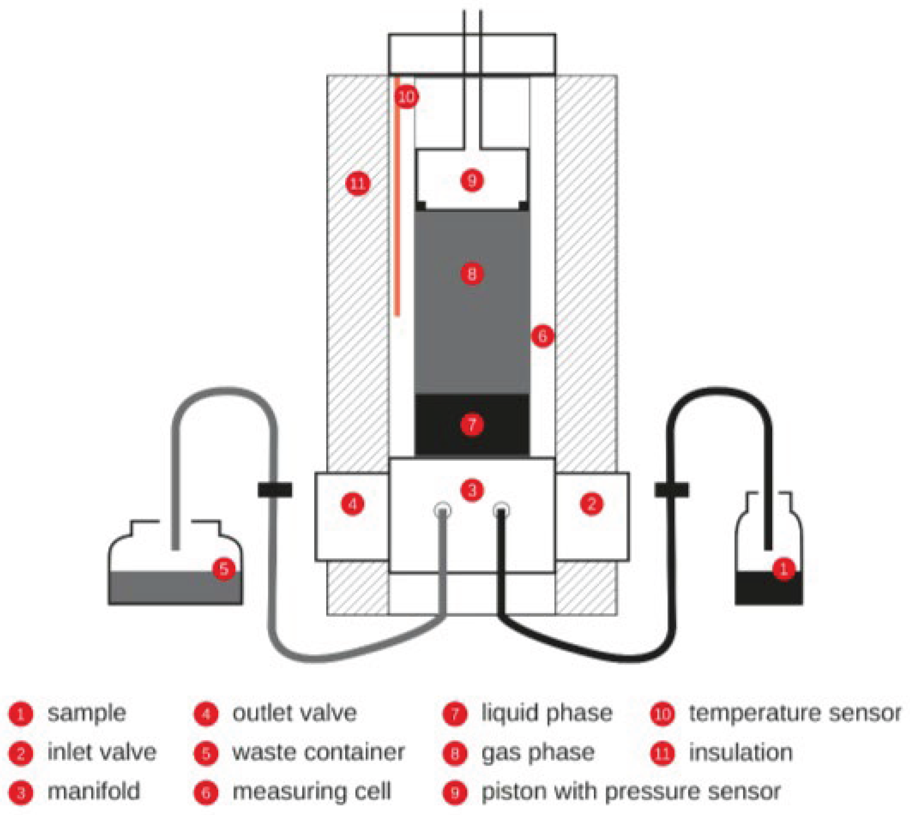
Figure 2.
Apparatus used for reflux experiment.
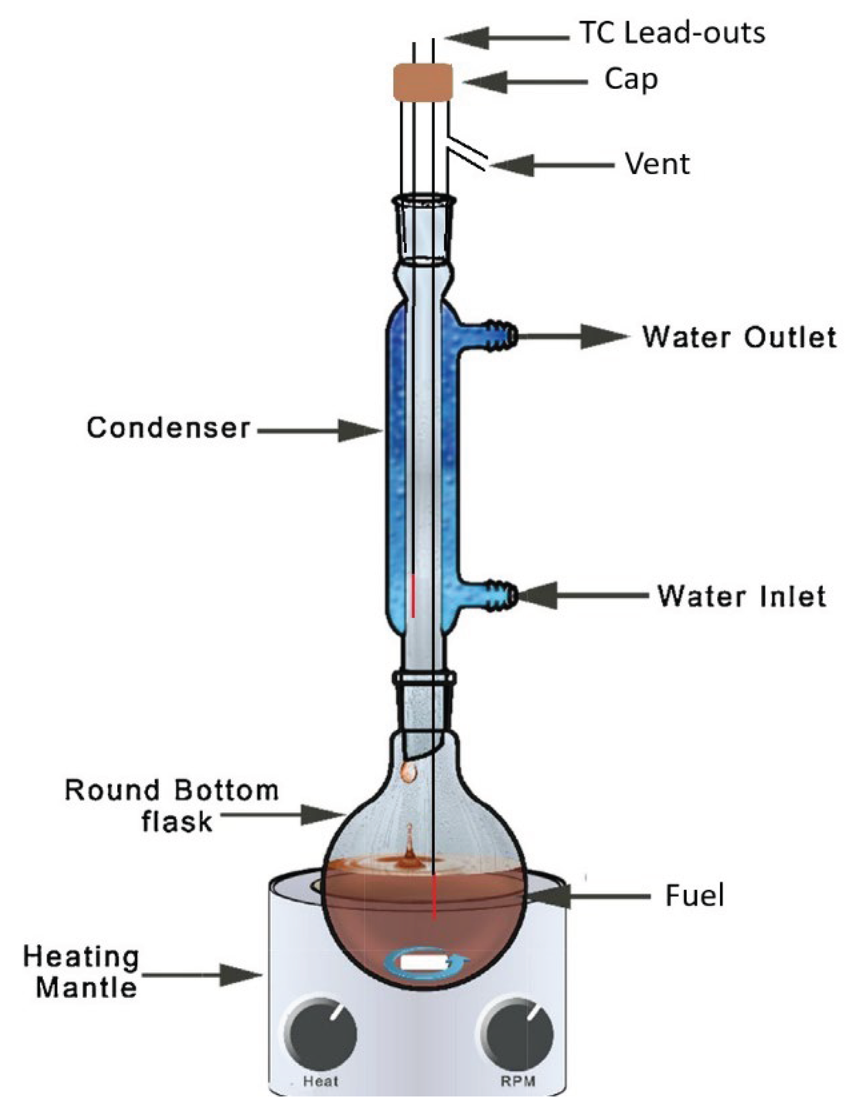
Figure 3.
Apparatus used for distillations.
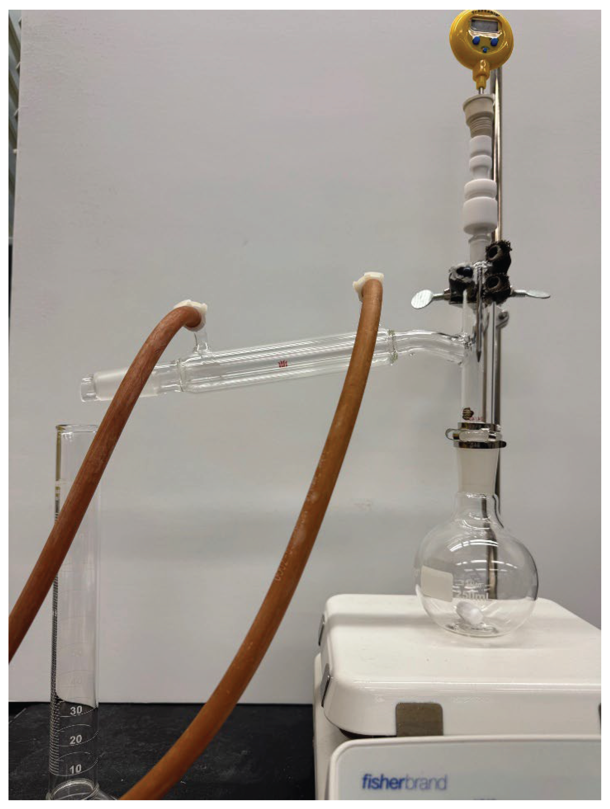
Figure 4.
Vapor Pressure Model Tuning Results. Filled symbols correspond to measurements. Curves correspond to model predictions.
Figure 4.
Vapor Pressure Model Tuning Results. Filled symbols correspond to measurements. Curves correspond to model predictions.
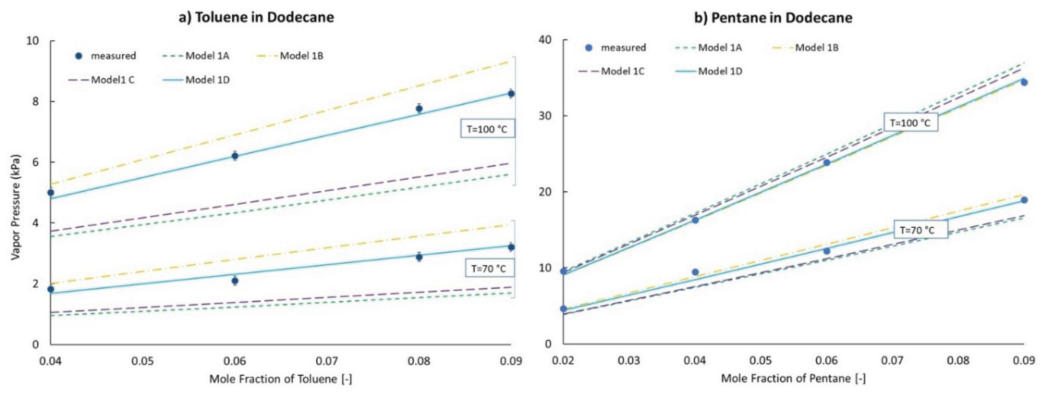
Figure 5.
Tuned Vapor Pressure Model Comparisons. Filled symbols correspond to measurements. Curves correspond to model predictions.
Figure 5.
Tuned Vapor Pressure Model Comparisons. Filled symbols correspond to measurements. Curves correspond to model predictions.
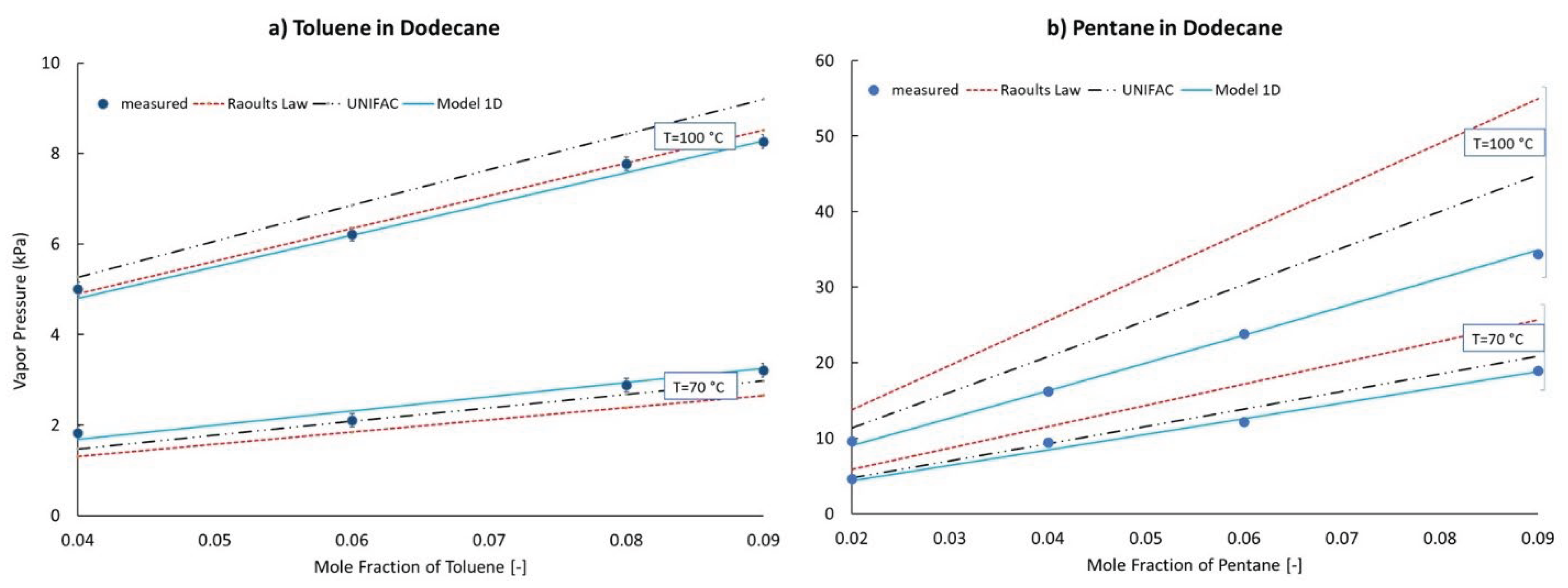
Figure 6.
Measured and Predicted Vapor Pressures of Ternary Mixture. Filled symbols correspond to measurements. Curves correspond to model predictions.
Figure 6.
Measured and Predicted Vapor Pressures of Ternary Mixture. Filled symbols correspond to measurements. Curves correspond to model predictions.
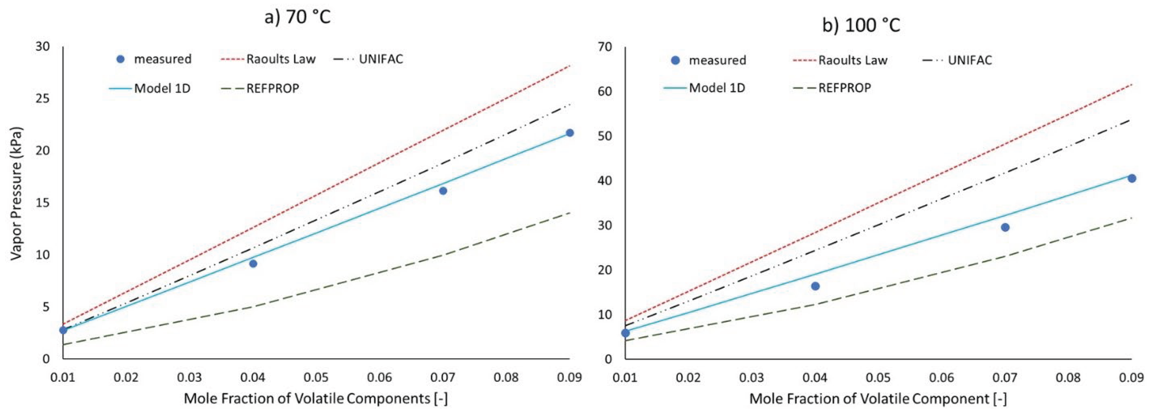
Figure 7.
Measured and predicted liquid temperature of refluxing mixture of cyclohexane and o-xylene in tetradecane.
Figure 7.
Measured and predicted liquid temperature of refluxing mixture of cyclohexane and o-xylene in tetradecane.
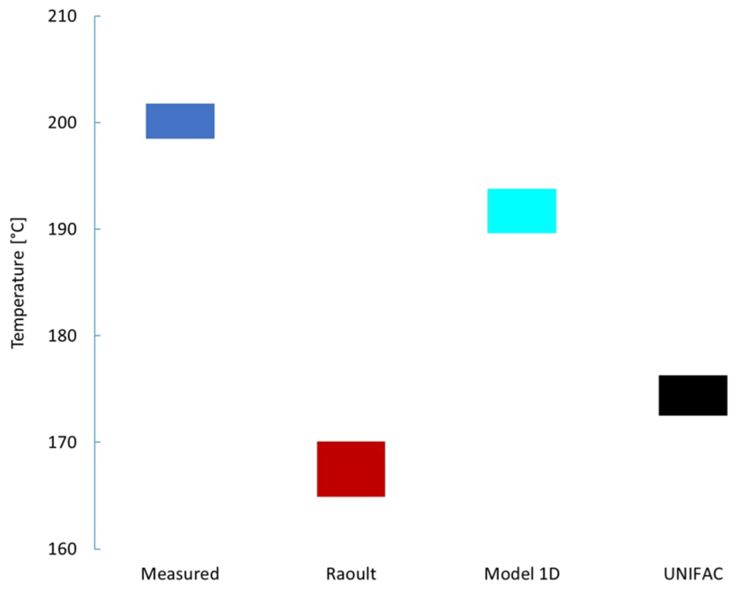
Figure 9.
Measured and predicted distillation curve of a mixture of cyclohexane and o-xylene in tetradecane. Filled symbols correspond to measurements. Open symbols correspond to corrected measurements. Curves correspond to model predictions.
Figure 9.
Measured and predicted distillation curve of a mixture of cyclohexane and o-xylene in tetradecane. Filled symbols correspond to measurements. Open symbols correspond to corrected measurements. Curves correspond to model predictions.
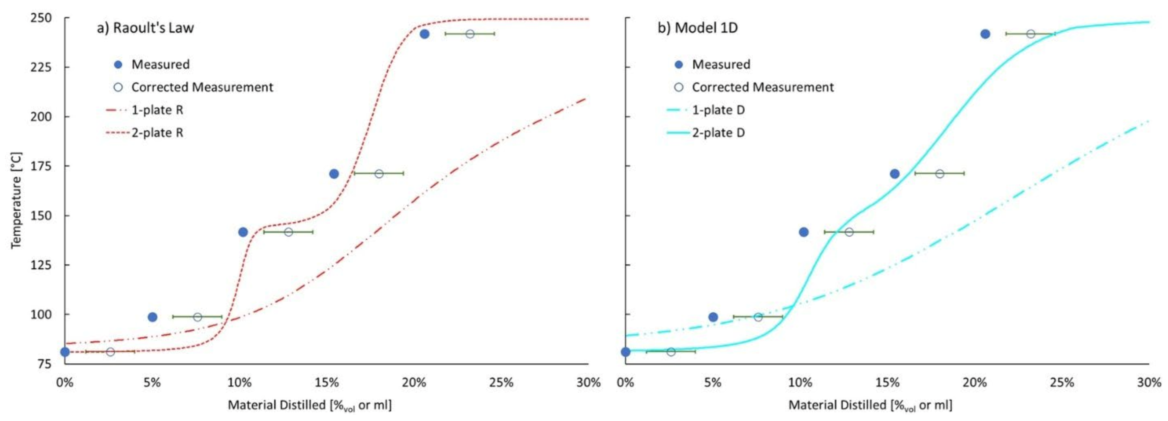
Figure 10.
Measured and predicted distillate composition of a mixture of cyclohexane and o-xylene in tetradecane. Filled symbols correspond to measurements. Open symbols correspond to corrected measurements. Curves and x’s correspond to model predictions. Green symbols and curves correspond to cyclohexane. Blue corresponds to o-xylene. Yellow corresponds to n-tetradecane.
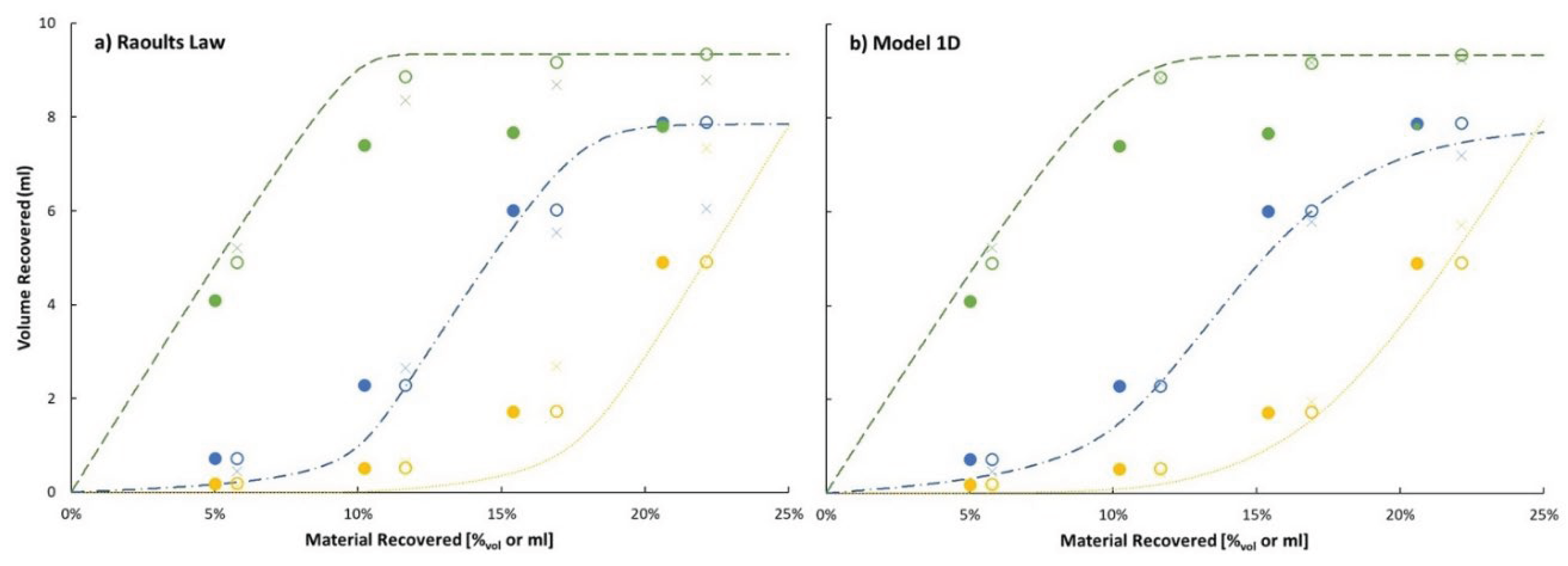
Figure 11.
Measured and predicted distillation curve of a mixture of isooctane and o-xylene in tetradecane. Filled symbols correspond to measurements. Open symbols correspond to corrected measurements. Curves and x’s correspond to model predictions.
Figure 11.
Measured and predicted distillation curve of a mixture of isooctane and o-xylene in tetradecane. Filled symbols correspond to measurements. Open symbols correspond to corrected measurements. Curves and x’s correspond to model predictions.
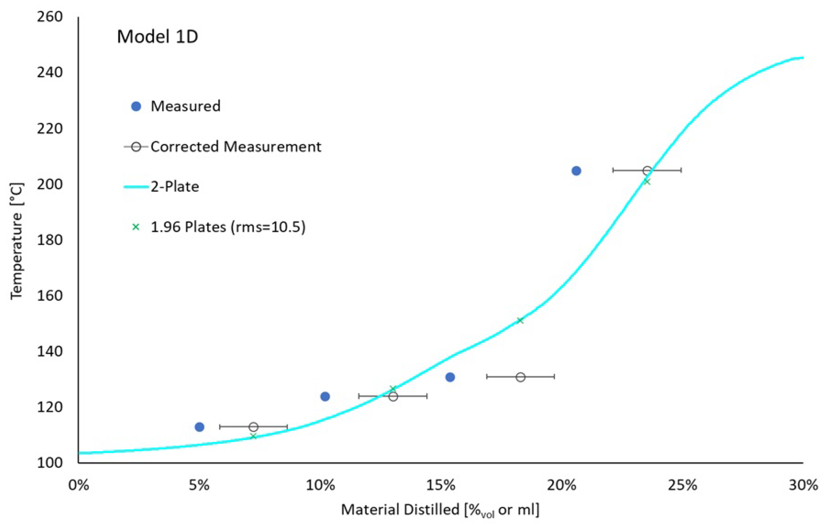
Figure 12.
Measured and predicted distillate composition of a mixture of isooctane and o-xylene in tetradecane. Filled symbols correspond to measurements. Open symbols correspond to corrected measurements. Curves and x’s correspond to model predictions. Green symbols and curves correspond to isooctane. Blue corresponds to o-xylene. Yellow corresponds to n-tetradecane.
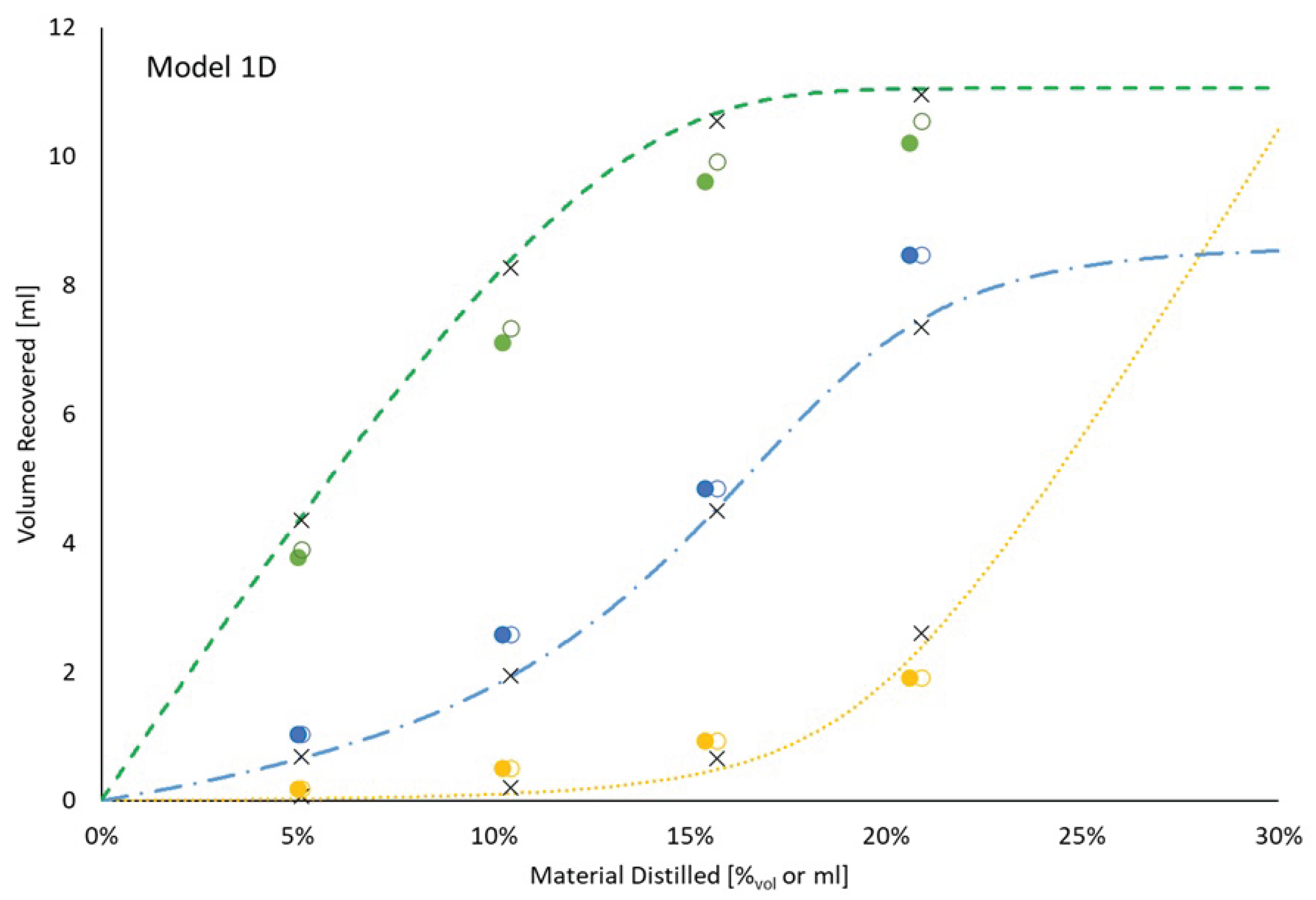

Table 1.
Fundamental UNIFAC parameters used in this work.
| Molecular Group | vdW volume | vdW surface area | ||
|---|---|---|---|---|
| -CH3 | 0.9011 | 0.848 | - | - |
| -CH2- | 0.6744 | 0.540 | - | - |
| arCH | 0.5313 | 0.400 | - | - |
| arC-CH3 | 1.2663 | 0.968 | - | - |
| CH2 :: arCH | - | - | 32.08 | 15.26 |
| CH2 :: arC-CH3 | - | - | 26.78 | -15.84 |
| arCH :: arC-CH3 | - | - | 167.0 | -146.8 |
Table 2.
Materials used in hydrocarbon mixtures.
| Name | Normal Boiling Point, °C [23] | Supplier | Purity (%) |
|---|---|---|---|
| n-Pentane | 36.0 | Thermo Scientific | 99 |
| cyclohexane | 80.8 | Fisher Scientific | 99.8 |
| n-heptane 1 | 98.4 | Alpha Aesar | 99 |
| isooctane | 99.2 | Sigma Aldrich | 99.5 |
| toluene | 110.6 | Thermo Scientific | 99.7 |
| ethylbenzene 1 | 136.2 | Thermo Scientific | 99 |
| o-xylene | 143.8 | TCI | 98 |
| n-nonane 1 | 150.6 | Thermo Scientific | 99 |
| n-propylbenzene 1 | 158.8 | Alpha Aesar | 98 |
| n-decane 1 | 174.1 | Thermo Scientific | 99 |
| n-dodecane (TCD) | 216.3 | Thermo Scientific | 99 |
| n-dodecane (WSU) 1 | Thermo Scientific | 99 | |
| n-tridecane 1 | 233.8 | TCI | 99 |
| n-tetradecane | 249.8 | Thermo Scientific | 99 |
1 These seven materials were part of a 10-component mixture that was distilled as part of this project. The data pertaining to that distillation is available by request to the correspondence author.
Table 3.
Antoine coefficients of selected materials: .
| Material | nBP (°C) | A | B (K) | C (K) |
|---|---|---|---|---|
| n-pentane | 36.0 | 3.9892 | 1070.617 | -40.454 |
| toluene | 110.6 | 4.0783 | 1343.9 | -53.77 |
| n-dodecane | 216.3 | 4.10549 | 1625.928 | -92.839 |
| cyclohexane | 80.8 | 3.96988 | 1203.526 | -50.287 |
| o-xylene | 143.8 | 4.12928 | 1478.244 | -59.076 |
| n-tetradecane | 249.8 | 4.13735 | 1739.623 | -105.616 |
| isooctane | 99.2 | 3.9368 | 1257.8 | -52.42 |
Disclaimer/Publisher’s Note: The statements, opinions and data contained in all publications are solely those of the individual author(s) and contributor(s) and not of MDPI and/or the editor(s). MDPI and/or the editor(s) disclaim responsibility for any injury to people or property resulting from any ideas, methods, instructions or products referred to in the content. |
© 2025 by the authors. Licensee MDPI, Basel, Switzerland. This article is an open access article distributed under the terms and conditions of the Creative Commons Attribution (CC BY) license (http://creativecommons.org/licenses/by/4.0/).
Copyright: This open access article is published under a Creative Commons CC BY 4.0 license, which permit the free download, distribution, and reuse, provided that the author and preprint are cited in any reuse.


