
Submitted:
02 October 2025
Posted:
02 October 2025
You are already at the latest version
Abstract
The Planetary Boundary Layer (PBL) remains a popular research topic, given its funda-mental role in the exchange of energy between the surface and the atmosphere. Under-standing the PBL's mechanisms can improve weather forecasting and climate and air quality modelling. This paper presents a PBL climatology based on 50 years of observa-tions (1973–2023) from the Bucharest Băneasa radio sounding station in Romania (inter-national identifier 15420). The Stull method was used to calculate the PBL height, which was extracted from the sounding at the Bucharest Băneasa observation point and consid-ers virtual potential temperature (θ_v). This incorporates the effect of humidity on air density. The analysis of climatological seasons (DJF, MAM, JJA and SON) based on PBL height series determined at 00 and 12 UTC using RAOB software revealed that the mixed layer height, as calculated by the Stull method, mainly captures the nocturnal Stable Boundary Layer (SBL) at 00 UTC and highlights the mixed layer (ML) at 12 UTC. ERA5 reanalysis data were also used in parallel.
Keywords:
PBL height
; climatology
; Stull method
; sounding
; ERA 5
1. Introduction
The troposphere is the most important layer of the Earth’s atmosphere. The Earth’s atmosphere is 80 percent troposphere, and it is bounded at the top by a layer called the tropopause. This boundary is marked by a temperature inversion in some areas and isothermal conditions in others. Although it extends approximately 11 km, with variations in height in the polar and equatorial zones, only 20 per cent of the troposphere is made up of the planetary boundary layer. This is the lowest part of the troposphere that is directly influenced by the Earth’s surface, responding in a matter of hours or less to forcing mechanisms. The thickness of the PBL varies over time and space depending on mechanisms including heat transfer, friction force and pollutants, as well as land use and landforms [2,4]. The PBL’s thickness varies with the time of day, involving a diurnal variation in thickness. Since water has a high heat storage and absorption capacity and there are no significant temperature changes, the depth of the PBL varies slowly over seas and oceans during the diurnal cycle. Only large-scale air advection and vertical movement can produce changes in PBL depth over the oceans. The depth of the PBL depends on the pressure regime, both over the oceans and over land. In high-pressure regimes, the PBL is thinner due to downdrafts and subsidence, which are specific to this regime. The situation is different in the case of a low-pressure regime. As a result of upward movements, the PBL can reach high altitudes in the troposphere [2].
Unlike over large bodies of water, the PBL structure over land varies throughout the day. In areas under high pressure, the PBL structure is well-defined during the diurnal cycle [2,3,4,5,6,7,8,9,10]. These are the stable layer, the residual layer and the mixed layer [2,8,9]. During the day, the thickness is influenced by cloud cover and solar radiation [2]. At night, radiative cooling causes the PBL to decrease in thickness, resulting in the layer near the surface remaining stable and forming a stable boundary layer. As the day progresses, the PBL thickness increases due to increased solar radiation and, consequently, convective processes [2,5,6,8]. This is known as the convective boundary layer (CBL), and understanding its structure is important for weather forecasting [7].
Convective processes generate turbulence in the mixed layer, with radiative cooling and heat transfer between different surfaces acting as sources of convection [2,5,7]. If there is no cold air advection, the turbulent movements weaken after sunset, forming a residual layer [2,5,8]. As it advances into the night, a stable layer forms at the bottom of the residual layer where it contacts the ground. In this layer, turbulence is very weak, and the air is stable [2,8].
There are several methods of determining the height of the PBL, each of which provides different information about it. In 1964, Holzworth conducted a foundational study on the determination of the mixed layer height using radiosonde observations [11]. This was followed by studies that improved and slightly modified his method [2,12,13], which involved adding an excess temperature to the surface temperature to account for measurement uncertainties [11]. One widely used method for determining PBL height from radiosonde data is the parcel method, also known as the Holzworth method. This method does not require the wind profile and is based on the intersection point of the dry adiabatic temperature starting from the surface and the profile temperature. This intersection point is interpreted as the equilibrium level of a rising parcel [9,10]. However, this method is subject to a high degree of uncertainty because it depends on the surface temperature.
Radiosonde data, which is widely used at most stations, is only available at the reference times of 00:00 and 12:00 UTC [6,9]. Therefore, comparisons with model estimations can only be made at these times. The uncertainty associated with this method is related to the nocturnal boundary layer, since no universal correlation has been found between wind, humidity and temperature profiles and turbulence. Several criteria are involved in interpreting the profiles of these parameters. This method can also be expensive [9]. Estimating the PBL height from radiosonde data can be subjective, as it is identified either by a temperature inversion or by a significant reduction in moisture in the profile [2].
Another approach to determining the PBL height is the bulk Richardson number method. This method assumes that the limit is reached when the Richardson number reaches a certain threshold value. The most used thresholds are 0.5 and 0.25 [14]. The bulk Richardson number is highly variable because the PBL is thermally stratified [14]. In their paper on PBL climatology over Europe and the United States, Seidel et al. (2012) conclude that the bulk Richardson number method is the most suitable for climatological studies [15]. Consequently, many studies use this approach [16,17,18].
The variation in PBL height can also be determined by using aircraft and remote sensing techniques. These techniques have both advantages and disadvantages [19]. For example, aircraft may only be used during the day, but they have the advantage of being able to operate a variety of sensors and cover large areas [9]. Other techniques used include lidar, sonar and Doppler radar/wind profiling [9,19]. Although Seibert considered these methods to be expensive, they offer the great advantage of enabling continuous monitoring of height variation over an entire diurnal cycle.
There are climatological studies on PBL height at the country/regional [4,5], continental [15,20,21,22,23] and global [24,25] levels. In his work (2013), Zhang observes a significant increase in PBL height in most regions of Europe in all seasons. Regarding the daily trend, he found a strong positive correlation between PBL height and surface temperature, as well as a strong negative correlation between PBL height and surface relative humidity.
Although there are numerous studies at the continental level, they do not cover re-gion of Romania, hence the importance of this updated climatological study.
2. Materials and Methods
2.1. ERA5 Reanalysis
The ERA5 reanalysis, developed by the European Centre for Medium-Range Weather Forecasts (ECMWF), is the fifth generation of global atmospheric reanalysis products and forms part of the Copernicus Climate Change Service (C3S). Designed to replace ERA-Interim, this dataset corrects its known limitations and provides a more comprehensive, high-resolution reconstruction of the global climate and atmospheric conditions from 1979 to the present [26]. The improvements are substantial: ERA5 provides hourly output instead of six-hourly; increases horizontal resolution to approximately 31 km; enhances vertical resolution through the use of 137 model levels; assimilates a significantly larger volume of observational data; and introduces uncertainty estimates via ensemble runs [27]. These changes make ERA5 more precise and versatile for a wide range of scientific, operational and societal applications [28]. ERA5 is based on the Integrated Forecast System (IFS), specifically Cycle 41r2, and employs a four-dimensional variational data assimilation (4D-Var) method. This assimilation system integrates various observational data sources with a short-range forecast, known as the background or first guess. Through a cost minimization process, the system constructs an atmospheric analysis that balances observations and model physics over a 12-hour assimilation window. Observations are assimilated dynamically, and their biases are corrected in real time using advanced techniques such as variational bias correction (VarBC) [29]. This approach ensures consistency in space and time, as well as improved physical realism compared to older reanalyzing.
The volume and diversity of observational data used in ERA5 are unmatched by previous reanalyses. While ERA-Interim assimilated around 750 000 observations per day in 1979, by 2018 ERA5 incorporated more than 24 million daily observations [26]. These include satellite radiance measurements from instruments such as TOVS, AIRS, IASI and AMSU, as well as in situ observations from radiosondes, aircraft, surface stations, ships and buoys. Additional datasets include ocean altimetry, snow depth and soil moisture. The assimilation system applies dynamic bias corrections, particularly to satellite radiances, to ensure consistency over time despite the evolution of the global observing system. ERA5 provides users with highly detailed outputs, offering a horizontal resolution of 0.25 degrees (approximately 31 km), 137 vertical levels extending up to 0.01 hPa (around 80 km in altitude), and an hourly temporal resolution. This represents a significant improvement on the 6-hourly data and coarser resolution of ERA-Interim. Furthermore, ERA5 provides a 10-member ensemble of data assimilations (ERA5-EDA), offering uncertainty estimates every three hours [27]. These ensemble data are particularly valuable in areas with sparse observations or during periods with less reliable data, as they provide users with a quantitative measure of confidence in the reanalysis fields. When validated against independent observations, ERA5 consistently outperforms ERA-Interim. Temperature and wind fields show stronger agreement with radiosonde and aircraft data, and ocean wave heights match buoy measurements more closely. Precipitation fields in ERA5 also correlate better with global observational datasets such as GPCP [28]. Furthermore, ERA5 is more successful at capturing extreme weather events, including storms, heatwaves and droughts, offering better temporal and spatial precision. Climate signals, such as tropospheric warming and stratospheric cooling, are preserved more accurately. However, a few known issues persist. For instance, the upper stratosphere shows artificial warming around the year 2000 due to changes in satellite data assimilation. Additionally, mesospheric winds are often overestimated in early periods due to physical limitations in the model [30].
Careful consideration of how the dataset is constructed is required when interpreting ERA5 data. Each analysis field is the result of a synthesis of model dynamics and observational data, with the weighting determined by the level of confidence in each. Therefore, long-term trends can be affected by changes in the observational system, particularly in the earlier decades when satellite coverage was more limited [31]. Users must therefore exercise caution when analysing trends across decades and ensure that they account for artificial discontinuities or shifts due to changes in data assimilation. ERA5 provides deterministic estimates as well as ensemble-based measures of uncertainty, which can be used to assess confidence in variables such as wind, temperature or PBL height in data-sparse regions. Differences between ERA5 and other reanalysis products stem from a variety of sources. One key factor is the use of different numerical weather prediction models and physics schemes. For instance, ERA5 turbulence, radiation, and land-surface interaction models are distinct from those used in MERRA-2, JRA-55, or NCEP reanalyses. Additionally, the assimilation systems vary; ERA5 uses 4D-Var, whereas others use 3D-Var or hybrid systems. Other differences arise from the diversity of assimilated observations, differences in spatial and temporal resolution, and distinct bias correction strategies. Even within ERA5, subtle discontinuities can emerge over time due to the addition or removal of satellite instruments or changes in assimilation configuration [32]. Therefore, cross-comparisons between reanalyses must be conducted with attention to methodological compatibility and data lineage. ERA5 has quickly become a foundational dataset for a wide range of scientific and operational domains. It is employed in climate change detection, attribution studies, weather prediction initialization, air quality modelling, renewable energy assessment, hydrological forecasting, and increasingly, machine learning applications in meteorology and climatology. Its combination of high temporal resolution, rich vertical structure and uncertainty quantification makes it an exceptionally useful tool for research and decision-making. Its enhanced depiction of the planetary boundary layer also facilitates research into surface-atmosphere coupling, which is crucial for modelling urban heat, wind energy, pollution dispersion and agricultural productivity.
In summary, ERA5 is a significant improvement on ERA-Interim in almost every respect. It covers a longer period (from 1979 onwards, with extensions planned back to 1950), has finer horizontal and vertical resolution, provides hourly outputs and assimilates a much larger volume of observational data. It also includes ensemble-based uncertainty estimates. These upgrades establish ERA5 as the most advanced and detailed global reanalysis currently available, positioning it as a central resource for understanding the Earth’s atmosphere on weather and climate timescales.
2.2. Planetary Boundary Layer (PBL) in ERA5
One of the key improvements in ERA5 is its enhanced representation of the planetary boundary layer (PBL). The PBL is the lowest portion of the atmosphere and is directly affected by surface processes such as turbulence, heat exchange and moisture fluxes. The PBL in ERA5 has significantly better vertical resolution: around 10 to 15 of the 137 model levels are located within the first two kilometres of the atmosphere. This denser vertical structure enables a more accurate depiction of boundary-layer dynamics, such as the formation of inversion layers or the daily cycle of mixing. ERA5 also uses upgraded turbulence parameterisations and improved coupling with the land surface model (CHTESSEL), resulting in more realistic surface-atmosphere interactions. When validated against radiosonde-derived estimates of PBL height, ERA5 performs notably better than previous reanalyses such as MERRA-2 or JRA-55 [33,34]. However, it still exhibits a tendency to underestimate daytime convective PBL heights by approximately 130 metres.
In ERA5, the PBL height is expressed in metres and is provided as a single-level hourly field with a spatial resolution of approximately 0.25 degrees (around 31 km) [26]. Rather than relying on turbulent kinetic energy (TKE), ERA5 determines PBL height using the bulk Richardson number method [35].
The bulk Richardson number is a dimensionless value that compares the stability of the atmosphere, as determined by thermal stratification, with the turbulence generated by wind shear [36]. The process begins by taking the lowest model level — typically around 10 metres above the surface — as the reference point. These model levels represent the atmosphere in a weather model such as ERA5, and are the vertical layers used inside it. These levels follow the terrain near the surface and the pressure levels higher up, enabling detailed calculations, particularly close to the ground [37]. The model then calculates the bulk Richardson number for each level aloft, moving upwards through the atmosphere from this surface level. The PBL top is identified as the lowest model level at which the bulk Richardson number exceeds the critical threshold of 0.25 [38]. If this threshold falls between two model levels, the height is determined by linear interpolation. This threshold is not arbitrary; it stems from empirical findings linking values of the bulk Richardson number below 0.25 to turbulent, well-mixed conditions within the boundary layer and values above 0.25 to stable, stratified layers where turbulence typically ceases [36]. To enhance accuracy, the calculation of the bulk Richardson number incorporates the virtual potential temperature, considering both temperature and humidity [36]. The method is based on physical principles: if the temperature and wind shear gradients are weak, the bulk Richardson number may remain below 0.25 across multiple layers, indicating a deep, well-mixed boundary layer. Conversely, in cases of strong night-time cooling near the surface, the bulk Richardson number can exceed 0.25 within a few hundred metres, resulting in a very shallow nocturnal boundary layer [39].
In practice, ERA5 uses this diagnostic method at each model time step to generate a gridded, hourly output field for boundary layer height. However, it does not store the full Richardson number profile; only the resulting height value is archived. This methodology is based on the ECMWF Integrated Forecasting System (IFS) and PBLH computation occurs during post-processing using the model wind and temperature fields [26,37]. Although the IFS model includes a turbulence closure scheme based on TKE, this is not employed to determine the PBLH in ERA5.
Despite its strengths, the ERA5 PBLH product has certain limitations. It is a diagnostic value, not a direct observation, and the bulk Richardson number method may underperform in situations involving weak shear or complex terrain, where turbulence may persist above 0.25 [39]. Furthermore, estimates of PBL height can vary significantly depending on the diagnostic method employed; while ERA5 relies on the Richardson number approach, other frameworks may use TKE thresholds or buoyancy criteria [38].
2.3. Planetary Boundary Layer (PBL) in RAOB
The aero sounding station was initially located in Mogoșoaia in the 1960s and 1970s, operating until it was relocated to Afumați in 1997–1998. The Afumați Meteorological Station is located approximately 15–17 km away from the old Mogoșoaia location as the crow flies. At the new location, radiosonde observations are still carried out at synoptic times of 00:00 and 12:00 UTC. To ensure continuity of the time series and avoid interruptions to the observational database initiated in the 1960s and 1970s, the station retained the same international call sign (15420 – Bucharest-Băneasa Meteorological Station). The relocation was carried out in compliance with the norms and recommendations of the World Meteorological Organization (WMO), with the equipment being transferred from north-west to north-east Bucharest [40].
According to the literature, researchers are encouraged to define the height of the planetary boundary layer using the methods and instruments available to them [9]. According to the Stull method, the height of the planetary boundary layer (PBL) is defined as the altitude at which the virtual potential temperature of an air parcel lifted adiabatically from the surface becomes equal to the ambient virtual potential temperature profile, thereby marking the upper limit of the convective mixed layer [36,41,42].
The height of the planetary boundary layer (PBL) was determined using the Stull (1991) method implemented in the RAOB 7.0 (RAwinsonde OBservations) program, which provides the PBL’s numerical value and graphical representation on a Skew-T diagram. It is also interactive software for analysing aerological soundings, capable of decoding and processing data in WMO, BUFR, GRIB and other standardised formats. The programme integrates a wide range of thermodynamic and dynamic algorithms for analysing the vertical structure of the atmosphere. These include modules dedicated to calculating significant levels (LCL, CCL and LFC), instability indices and parameters associated with turbulence and vertical transport [43]. This method was chosen because it is independent of numerical models, is based on direct observational data and provides a more realistic estimate of PBL height in environments with high humidity than other methods. It has also been demonstrated to be applicable in operational meteorology and pollutant dispersion studies.
Thus, determining the PBL height using the Stull method and the RAOB program provides a robust estimate of the mixed layer depth, as well as solid information for evaluating vertical transport and atmospheric dispersion processes.
This method is derived from parcel theory and static stability analysis and is based on the virtual potential temperature (θ_v) profile.
The calculation procedure consists of several steps. First, the virtual potential temperature of the surface is determined from the observed temperature and humidity at ground level. The virtual potential temperature considers the effect of water vapour on air density. Next, the movement of the surface particle along the vertical profile is tracked, assuming an adiabatic rise until it intersects with the ambient medium. The static equilibrium level is then identified as the altitude at which the θ_v profile of the surface particle is equal to that of the ambient medium. This intersection marks the upper limit of the mixed layer and, consequently, the height of the PBL. Under conditions of convective instability, this method determines the depth of the turbulent layer (mixed layer) between the surface and the intersection level. In situations involving low stable layers or inversions, the method may indicate low PBL values, reflecting inhibited vertical mixing. Compared to the Holzworth method, which uses only potential temperature (θ_v), the Stull method provides a more realistic estimate of the PBL in humid environments, where the effect of water vapour is significant and neglecting it leads to an underestimation of the mixed layer height.
3. Results
For 12 UTC (see Figure 1 and Figure 2), the average PBL height in the winter season (DJF) is 545 m according to the ERA5 data and 601 m according to the Stull method. In the winter season, both methods indicate low PBL heights. However, the values obtained by the Stull method are higher than those obtained from ERA5.
In spring (MAM), the average PBL height is 1274 m according to the ERA5 data and 1323 m according to the Stull method.
ERA5 data show an increasing trend in PBL height for the MAM season, while the Stull method shows similar average values. Predominantly below-average values are observed until the 1990s, after which higher-than-average values predominate.
In summer (JJA), the average PBL height is 1494 m according to the ERA5 data and 1662 m according to the Stull method.
For the warm season, both the ERA5 data and the Stull method indicate a clear intensification of the PBL height, which is correlated with intense warming and convection. ERA5 indicates an increase after 2000. The Stull method shows below-average values until the 1990s, as with the ERA5 values. After this, higher values are observed, but the data are more dispersed.
In autumn (SON), the average PBL height is 936 m according to the ERA5 data and 1021 m according to the Stull method. SON is characterised by moderate average PBL heights, with similar values between the two methods and no clear trend.
Winter is characterised by generally low values close to the climatological mean, with higher dispersion in the Stull method. ERA5 shows a slight increase in the frequency of years with below-average PBL, but the signal remains modest. The picture is slightly noisier in Stull: above-average values predominate in the 1970s–1980s, followed by a period of decrease in the 1990s and a redistribution with variations around the mean value.
Spring presents a much clearer signal. In ERA5, most years before 2000 have values close to or below average, with a few exceptions. After 2000, however, years with a PBL above the multi-year mean frequently dominate. This increase is particularly evident between 2000 and 2008, suggesting an intensification of convective processes. In Stull, the distribution is more variable, but the general trend shows a similar shift towards higher values over the past two decades.
Summer is the season with the most pronounced differentiation. In ERA5, below-average values predominated before 2000, but above-climatological values clearly predominated after this year, with notable maxima around 2007 and 2008. This behaviour reflects an increase in the intensity of thermal convection against a background of climate warming. In Stull, the pattern is similar, but with sharper variations, indicating greater methodological sensitivity to extreme years.
Autumn is more balanced: in the ERA5 dataset, an alternating succession of above- and below-average years is observed before 2000. After 2000, the frequency of above-climatological years increases slightly, but without a robust signal. In the Stull method, variability is high, but the same moderate long-term increasing trend is clearly observed after 2000.
The Stull method shows a robust positive trend after 2000, with the strongest increase in summer and spring. This suggests an intensification of convective processes on a climatological scale. The ERA5 series at 12 UTC partially confirms the increasing trend, but with more moderate values and reduced variability.
For 00 UTC (see Figure 3 and Figure 4), the average PBL height in the winter season (DJF) is 312 m according to the ERA5 data and 454.11 m according to the Stull method. While the ERA5 data shows some stability with moderate variations, the Stull method captures larger extremes with higher variability.
In spring (MAM), the average PBL height is 308 m according to the ERA5 data and 423 m according to the Stull method. The ERA5 data show moderate variations around the average value that are somewhat symmetrical to it, while the Stull method highlights episodes in which values below the seasonal average predominate.
In the summer season (JJA), the average PBL height value obtained from the ERA5 data is 250 m, while the average PBL height value obtained using the Stull method is 311 m. The ERA5 values show moderate variations around the average, with successive increases and decreases every 10–15 years, while the Stull method predominantly produces above-average values until the 1990s, followed by values lower than the average.
The analysed data show that ERA5 has lower values than the Stull method, but these are more stable and the trends are insignificant. The Stull method produces higher PBL height values and greater variability, but without a clear trend.
During the cold season (DIF), the Stull method applied at 00 UTC yields higher mean values than ERA5, albeit with significant inter-annual variability. The significant negative trends observed (i.e. height values below the seasonal mean) reflect the deepening of the nocturnal stable layer (SBL), which is determined by persistent thermal inversions and intensified radiative cooling. During the period from the 1970s to the 1990s, there were years when the residual layer (RL) played a more significant role, as the heights were higher than the seasonal mean. It is worth noting that, since the 1990s, the mean values have mostly been below the seasonal mean. ERA5 remains approximately constant throughout this period, showing that the model diagnosis attenuates real variations. At 00 UTC, the residual layer (RL) plays a reduced role and the estimates capture almost exclusively the SBL.
In the transitional months (MAM), the Stull method shows a significant decrease after the 1990s, followed by an upward trend between 2015 and 2020. Meanwhile, the mean height in ERA5 remains relatively constant, with no notable trends. During this season, daytime RL often persists overnight, but the Stull method primarily identifies the depth of the SBL. The difference in values between the Stull method and ERA5 suggests that the reanalysis data does not fully capture the interaction between the RL and the SBL; direct estimates, however, highlight greater variability in stratification processes.
During the warm season, the Stull method shows a decrease in the mean value after the 1990s, accompanied by a robust negative trend. ERA5 shows lower values, with a more stable mean over time. Summer is the season with the strongest contrast between the diurnal mixed layer (ML) and the thin SBL formed at night.
During the transition to winter (SON), the Stull method shows clear decreases after the 1990s, whereas ERA5 indicates a slight increase. Autumn is characterised by the contrast between days that are still convective enough for rain-free convection (RFC) and cold nights that favour a persistent surface boundary layer (SBL). Stull estimates reflect large amplitude and pronounced variability, whereas ERA5 attenuates these fluctuations.
The data confirm that, at 00 UTC, the Stull method primarily captures the SBL, which shows significant decreasing trends after the 1990s, followed by stabilisation. Meanwhile, ERA5 maintains a constant and homogeneous regime. Although the residual layer (RL) is present, especially in spring, summer and autumn, it is not directly represented in the 00 UTC series because the applied algorithm prioritises SBL.
When the average values obtained by the Stull method (12 UTC measurements) are compared with those from the ERA5 data (also 12 UTC measurements) for Bucharest-Băneasa, it is found that, for the lowest values of PBL height from the observational data, the values from ERA5 are consistently higher in all months. Conversely, the highest layer height values from the observations are higher than those calculated with ERA5, capturing both the initiation of PBL formation and its maturity phase. There is an increased deviation from March to September (see Table 1 and Table 2).
For the minimum values (see Table 3), the values determined by the Stull method are lower than those in ERA5 in all months. This shows that the reanalysis data tend to overestimate the thickness of the nocturnal stable layer when it is poorly developed. For the maximum values (Table 4), the Stull method consistently yields higher values than ERA5. This suggests that ERA5 underestimates the maximum development of the nocturnal stable layer and only partially captures the intensification of the nocturnal inversion layer.
Therefore, the same trend observed at 12 UTC is confirmed. ERA5 smooths the extremes, providing higher values at the minimums and lower values at the maximums. This reflects the limitations of the reanalysis data in capturing the true variability of the planetary boundary layer.
4. Discussion
In the analysed interval for Bucharest, the lowest monthly PBL height values in ERA5, measured at 12 UTC, are found in January and December. This is because the average number of sunny days in these months is three, with the remaining days being partially or fully cloudy, which limits the PBL height. If the height is relatively uniform in December, lower values appear in January. The most notable of these were in 1985 (when 16 consecutive days with negative temperatures were recorded in Bucharest and it was declared the coldest winter in 40 years), 1990, 2002 and 2011, when the PBL height slightly exceeded 300 m.
The highest value was 775 m in January 2022. According to the European Union’s Climate Change Service, Copernicus, temperatures higher than climatological averages were recorded throughout Europe, including Romania, that month. According to this report, “glob-ally, January 2022 was 0.28 °C warmer than the average January in the 1991-2020 reference period and the sixth warmest January recorded to that date. At the European level, average temperature anomalies are generally larger and more variable than at the global level, the average temperature in January 2022 was 0.79 °C above the average of the 1991-2020 reference period” [43].
In Bucharest, the month began with temperatures over 10 degrees Celsius and sunny days.
The height of the PBL varies depending on the surface temperature and humidity. It increases when the surface temperature is high and humidity is low. In these conditions, sensible heat fluxes dominate latent heat fluxes, leading to an increase in buoyancy. As expected, the mixing depth begins to increase in March, a month generally characterised by changeable weather, with cold, wet days alternating with warm, sunny ones. This continues until October, with the most significant increases occurring from May to August in the first 25 years analysed (1973 to 2002). The year 1994 (with an average value of 1258 m recorded in March) was extraordinarily warm and amazed climatologists at the time. Few would have thought that there would be warmer years in the following 30 years. Significant warming began to be felt after 2002, when droughts and heatwaves became increasingly frequent. In the following 25 years, there were significant increases in PBL height in all summer months (June 2007: 2031 m; July 2007: 2258 m; August 2008: 2067 m). Moreover, these increases extend from the beginning of spring and continue until late autumn (March to September inclusive).
The increasing trend in PBL height in September can be associated with heatwaves that persist at the end of summer and affect Southeastern Europe. These heat waves, characterised by sunny days and high temperatures, have become more frequent and intense, as seen in 2007, 2012, 2015, 2017, 2020 and 2022.
In 2007, the maximum PBL values corresponded to three prolonged heatwaves: one in June (19–27 June), with an average value of 2031 m; one in July (15–25 July), with an average value of 2258 m, during which there was an uninterrupted heatwave; and one in August (23–25 August), with an average value of 1610 m. In 2012, the maximum PBL value in July (1906 m) can be interpreted as the result of advection of tropical warm air of North African origin, which was present over south-eastern Europe from the beginning of the month until 16 July. From June to September in 2015, there were five heatwaves, two of which covered most of July (between the 6th and 9th and the 16th and 30th) with values between 1600 and 1700 metres. In 2017, two heatwaves in August (at the beginning and end of the month) led to an increase in the PBL height in both August and September (with values between 1300 and 1600 m).
The summer of 2020 saw record temperatures, even in September, with an average value of 1510 m, when heatwaves reached as far as Russia, with temperatures of 30 °C in Moscow. The PBL depth remained high from April (with an average value of 2063 metres) until early October, reaching its maximum in July, August and September (with values between 1500 and 1900 metres, and an average value of 1962 metres in August).
According to the report published by the European Copernicus Climate Change Service, the summer of 2022 was declared the warmest ever recorded in Europe since the beginning of meteorological measurements. This dethroned the summer of 2021, which had previously been recorded as the hottest summer to that date (with values between 1600 and 1900 m, and an average value of 1974 m in July).
From 2008 to 2023, August was often warmer than July, although July was generally warmer than the following month.
Bucharest is a metropolis located inland, far from the influences of water, in contrast to other European cities used as observation points in the literature on the analysed topic. These other cities are located in the vicinity of large bodies of water (Mediterranean Sea: Brindisi, Trapani, Cagliari, Gibraltar; Bay of Biscay: Bordeaux; Atlantic Ocean: Valencia) [1]. The temperate climate of Bucharest is dictated by its geographical location in the Carpathian-Balkan basin, respectively in the Romanian Plain [2], and the Afumați Meteorological Station is located at an altitude of 90 meters (with an indicative 15420 from Bucharest-Băneasa, as we explained why this convention was made). These cumulative aspects influence the local climate peculiarities.
Tumanov et al. (1999) even discuss differences in the main meteorological parameters within the metropolis, taking the meteorological stations at Băneasa and Filaret into account in their analysis. In his study, he observed a noticeable difference in cloudiness between the two stations. The presence of stratiform clouds at the meteorological station in the northern part of the city is attributed to the influence of the lake and the forest in that area. This phenomenon is said to occur more frequently in the mornings at the Băneasa meteorological station than at the Filaret meteorological station. The author also analysed a case of a frontal passage on 17 April 1994. A compact system that was expected to pass over the city broke up as it passed over, regrouping after crossing the city [2].
The particularities induced by the local geography, in all its aspects, along with influences at the synoptic scale, are reflected in the climatology of the planetary boundary layer height above Bucharest. The temporal and spatial variability of this parameter can be clearly represented using heatmap graphs, which facilitate a complex yet consolidated analysis of the climatology of the planetary boundary layer height. As can be seen in Figure 5, which shows the PBL height resulting from ERA5 calculations, the months in the cold semester indeed present the lowest heights, ranging from 219 m to 368 m (average values). January is the month when the PBL reaches its lowest heights. In January, the northern half of the continent experiences tighter barometric gradients due to the deepening of the Icelandic Low. This leads to an intensification of atmospheric circulation in the north. In contrast, the south and the Romanian Plain typically see greater stability of the air masses. This is due to the formation of an anticyclonic belt, brought about by the union of the Siberian and Azores high-pressure systems.
Thus, cyclonic activity in the Mediterranean Basin weakens and circulation becomes less intense [3]. The transitional seasons (MAM and SON) exhibit similarities with regard to the height of the planetary boundary layer. In March, values range from 609 m to 1671 m, with the lowest value recorded in 2018. April is the month when the height has exceeded 2000 m on two occasions in the analysed data series (2063 m in 2020 and 2017 m in 2007). The lowest height was recorded in 2016 at 990 m, while May is characterised by values exceeding 1500 m. The maximum height was recorded in 1986 at 1865 m, and the minimum value does not drop below 1100 m, with an average value of 1144 m in 1980. As the Northern Hemisphere warms, the anticyclonic belt shifts northwards, the Icelandic Low weakens and the depression over Asia Minor becomes more influential. Consequently, the southern part of the continent experiences more intense circulation than the northern part [3]. During the warm season, the highest PBL height values are recorded, with July 2007 standing out from the other years in the analysed period with a maximum value of 2258 m.
The lowest height, 1011 m, is observed in June 1991. Starting in June, evident changes to the baric field are observed at continental level. The thermal low over Asia Minor deepens while the Siberian High weakens. The Icelandic Low weakens over the North Atlantic, resulting in weaker winds over northern Europe [3]. From September onwards, the values gradually decreased, with November showing the most homogeneous PBL height values across the entire analysed period, ranging from 409 m to 832 m.
November is the most stable month of the year due to the extension of the Siberian High ridge, which reaches as far as the western Alps. The ridges of the Azores High and the Siberian High merge to form a high-pressure belt positioned further south over the continent during the cold season than during the warm season. This configuration blocks circulation from the Mediterranean Sea towards Romania [3].
The heatmaps in Figure 5 and Figure 6, which are based on measurements from the observation point at Meteorological Station Afumați (15420 Bucharest Băneasa), also show a clear seasonal variability, with the highest PBL heights occurring during the summer months. This is a result of thermal convection that induces intense turbulence [4]. The greatest homogeneity is observed during the cold and transitional months. In the warm months, however, although there is a clear upward trend in PBL height, year-to-year homogeneity decreases. The highest PBL height was recorded in July 2007, with average values of 2258 m and 2794 m from ERA5 and the Stull method, respectively. The increase in PBL height is related to changes in other meteorological parameters in the Bucharest area, which influence the local climate. In his study, Tumanov S. et al. (1999) report a decrease in the number of foggy days and rainy days, a reduction in wind speed and an increase in relative humidity at the Băneasa and Filaret stations in the period 1961–1990 [2].
The ERA5 data (Figure 7) show a relatively uniform evolution of the boundary layer at night, with moderate height values (the multiannual monthly average is approximately 240–330 m, with seasonal variations). These values are typical of a stable nocturnal boundary layer (SBL), which develops through the radiative cooling of the surface. It is characterised by shallow depth and weak turbulence. The limited interannual variations suggest that the ERA5 reanalysis tends to ‘smooth out’ extremes and provide robust climatological averages. At the same time, higher values occasionally appear (above 500–600 m; for example, 540 m in October 2004 and 617 m in March 2002), which are interpreted as residual layers (RLs) formed during the day that did not dissipate completely after sunset. This behaviour indicates that ERA5 effectively captures both the SBL typical of calm and cold nights, and episodes of persistent RL, particularly during the transitional months of spring and autumn.
Estimates based on Stull’s method (Figure 8) show much greater variability in PBL height at night, with values ranging from a few hundred metres (multiannual monthly averages between 300 and 510 metres) to over 1000 metres (1116 metres in March 1984). This behaviour indicates that the method is more sensitive to local conditions (atmospheric circulation, stratification and mechanical forcing). The high values (800–1200 m; specifically 951 m in February 1984; 1,116 m in March 1984; 897 m in October 1987; and 974 m in November 1975) suggest that the method retains the signal of a strongly developed residual layer (RL) during the day, which dominates the nocturnal structure. In contrast, low values (200–400 m) correspond to a classic SBL formed under conditions of radiative cooling and stable stratification. Compared to ERA5, the Stull method accentuates these differences, providing a clearer distinction between the shallow SBL and the persistent RL. This is an important aspect for case studies and the evaluation of residual vertical transport events (e.g. pollutants and aerosols).
5. Conclusions
At 12 UTC, both the Stull method and the ERA5 reanalysis data capture the convective mixed layer (CML), with values in the order of kilometres for the warm and transitional seasons. The Stull method reveals greater extremes and variability, whereas the ERA5 provides a more consistent diagnosis with lower maximum limits.
The Stull series shows positive trends after 2000, which are particularly significant during the warm seasons (JJA and SON). This suggests an intensification of diurnal convection. By contrast, the ERA5 data only shows moderate increases until the 2000s, after which it stabilises.
The results suggest an increase in ML height after 2000, which is probably associated with an intensification of convection and a change in the regional energy regime. The differences between the Stull method and the ERA5 reanalysis data reflect methodological limitations: the Stull method is more sensitive to local and extreme processes, whereas the ERA5 data are less variable.
At 00 UTC, the values obtained by the Stull method primarily reflect the stable night-time layer (SBL). These values demonstrate significant variability and decreasing trends below average in all seasons. In contrast, ERA5 provides a more consistent diagnosis without any robust climatological signals currently.
The pronounced increases observed in the Stull method at 00 UTC during the 1970s–1990s disappear, indicating a possible change in the nocturnal stability regime. After 2000, the trends at 12 UTC are positive (especially during the warm seasons), suggesting an intensification of diurnal convection.
In terms of the differences between the methods, the Stull method produces estimates that reach higher maximum values than ERA5 but also exhibit much greater dispersion. In contrast, ERA5 limits extremes and smooths variability. This structural difference between the two methods is a key factor in interpreting the results.
Regarding the connection between the 00 and 12 UTC observations, the following can be stated: inter-annual correlations are weak or negative, particularly in summer. This confirms that the PBL height at 00 UTC cannot be used as a proxy for the residual layer (RL). The diurnal amplitude between the 00 and 12 UTC observations is primarily determined by the ML depth rather than the nocturnal structure.
The results emphasise that the processes governing the diurnal PBL (convection) and the nocturnal PBL (radiative cooling and inversions) are fundamentally different. The climatological analysis must therefore treat these regimes separately. To characterise the RL, other dedicated methods that explicitly distinguish between the SBL and the RL must also be applied.
Author Contributions
Conceptualization, Adrian Timofte, Diana Bostan and Marius Cazacu; Data curation, Adrian Timofte, Diana Bostan, Cosmina Apetroaie, Ingrid Miclăuș and Marius Cazacu; Formal analysis, Adrian Timofte, Cosmina Apetroaie, Ingrid Miclăuș and Marius Cazacu; Investigation, Adrian Timofte, Diana Bostan, Cosmina Apetroaie, Ingrid Miclăuș and Marius Cazacu; Methodology, Adrian Timofte, Diana Bostan, Cosmina Apetroaie, Ingrid Miclăuș and Marius Cazacu; Project administration, Adrian Timofte and Marius Cazacu; Resources, Adrian Timofte, Diana Bostan, Cosmina Apetroaie and Marius Cazacu; Software, Adrian Timofte, Diana Bostan, Ingrid Miclăuș and Marius Cazacu; Supervision, Adrian Timofte and Marius Cazacu; Validation, Adrian Timofte, Diana Bostan, Ingrid Miclăuș and Marius Cazacu; Visualization, Adrian Timofte, Diana Bostan, Ingrid Miclăuș and Marius Cazacu; Writing – original draft, Adrian Timofte, Diana Bostan, Cosmina Apetroaie and Ingrid Miclăuș; Writing – review & editing, Adrian Timofte and Marius Cazacu. All authors have read and agreed to the published version of the manuscript.
Funding
This work was financed by Smart Growth, Digitization and Financial Instruments Program (PoCIDIF) 2021-2027, Action 1.3 Integration of the national RDI ecosystem in the European and international Research Space, project “Supporting the operation of facilities in Romania within the ACTRIS ERIC research infrastructure”, SMIS code 309113.
Institutional Review Board Statement
Not applicable
Informed Consent Statement
Not applicable
Data Availability Statement
The raw data supporting the conclusions of this article will be made available by the authors without undue reservation.
References
- Speight, J. G. (2020). Water systems. Natural Water Remediation, 1–51. doi:10.1016/b978-0-12-803810-9.00001-2.
- Roland B. Stull, An introduction in boundary layer meteorology; Kluver Academic Publishers, Norwell. Mass, 1988; pp. 2-3.
- Heintzenberg, J. (1989), Fine particles in the global troposphere A review. Tellus B, 41B: 149-160. [CrossRef]
- Allabakash, S.; Lim, S. Climatology of Planetary Boundary Layer Height-Controlling Meteorological Parameters Over the Korean Peninsula. Remote Sens. 2020, 12, 2571. [CrossRef]
- Guo, J., Miao, Y., Zhang, Y., Liu, H., Li, Z., Zhang, W., Zhai, P. (2016). The climatology of planetary boundary layer height in China derived from radiosonde and reanalysis data. Atmospheric Chemistry and Physics, 16(20), 13309–13319. doi:10.5194/acp-16-13309-2016.
- Gu, J., Zhang, Y., Yang, N., & Wang, R. (2020). Diurnal variability of the planetary boundary layer height estimated from radiosonde data. Earth and Planetary Physics, 4(5), 1–14. doi:10.26464/epp2020042.
- De Wekker SFJ and Kossmann M (2015) Convective Boundary Layer Heights Over Mountainous Terrain—A Review of Concepts. Front. Earth Sci. 3:77. doi: 10.3389/feart.2015.00077.
- Chilson, P.B.; Bell, T.M.; Brewster, K.A.; Britto Hupsel de Azevedo, G.; Carr, F.H.; Carson, K.; Doyle, W.; Fiebrich, C.A.; Greene, B.R.; Grimsley, J.L.; et al. Moving towards a Network of Autonomous UAS Atmospheric Profiling Stations for Observations in the Earth’s Lower Atmosphere: The 3D Mesonet Concept. Sensors 2019, 19, 2720. [CrossRef]
- Seibert, P. (2000). Review and intercomparison of operational methods for the determination of the mixing height. Atmospheric Environment, 34(7), 1001–1027. doi:10.1016/s1352-2310(99)00349-0.
- Granados-Muñoz, M. J., F. Navas-Guzmán, J. A. Bravo-Aranda, J. L. Guerrero-Rascado, H. Lyamani, J. Fernández-Gálvez, and L. Alados-Arboledas (2012), Automatic determination of the planetary boundary layer height using lidar: One-year analysis over southeastern Spain, J. Geophys. Res., 117, D18208, doi:10.1029/2012JD017524.
- Stachowiak, Olga I. “Mixing height and Cloud Convection in the Canadian Prairies.” (2010).
- Garrett, A. J., 1981: Comparison of Observed Mixed-Layer Depths to Model Estimates Using Observed. J. Appl. Meteor. Climatol., 20, 1277–1283, . [CrossRef]
- Wotawa, G., and A. Stohl. “Boundary layer heights and surface fluxes of momentum and heat derived from ECMWF data for use in pollutant dispersion models-problems with data accuracy.” (1997).
- Zhang, Y., Gao, Z., Li, D., Li, Y., Zhang, N., Zhao, X., & Chen, J. (2014). On the computation of planetary boundary-layer height using the bulk Richardson number method. Geoscientific Model Development, 7(6), 2599–2611. doi:10.5194/gmd-7-2599-2014.
- Seidel, D. J., Zhang, Y., Beljaars, A., Golaz, J.-C., Jacobson, A. R., & Medeiros, B. (2012). Climatology of the planetary boundary layer over the continental United States and Europe. Journal of Geophysical Research: Atmospheres, 117(D17), n/a–n/a. doi:10.1029/2012jd018143.
- Van Dop, H., M. Krol, and B. Holtslag. “A global boundary-layer height climatology.” (1997).
- Batchvarova, E., and S-E. Gryning. “Use of Richardson number methods in regional models to calculate the mixed-layer height.” Air Pollution Processes in Regional Scale. Dordrecht: Springer Netherlands, 2003. 21-29.
- Jeričević, Amela, and Branko Grisogono. “The critical bulk Richardson number in urban areas: verification and application in a numerical weather prediction model.” Tellus A: Dynamic Meteorology and Oceanography 58.1 (2006): 19-27.
- Emeis, Stefan, Klaus Schafer, and C. H. R. I. S. T. O. P. H. Munkel. “Surface-based remote sensing of the mixing-layer height-a review.” Meteorologische Zeitschrift 17.5 (2008): 621.
- Zhang, Y., D. J. Seidel, and S. Zhang, 2013: Trends in Planetary Boundary Layer Height over Europe. J. Climate, 26, 10071–10076, . [CrossRef]
- Sánchez, E., C. Yagüe, and M. A. Gaertner. “Planetary boundary layer energetics simulated from a regional climate model over Europe for present climate and climate change conditions.” Geophysical research letters 34.1 (2007).
- Esau, Igor, and Svetlana Sorokina. “Climatology of the arctic planetary boundary layer.” Atmospheirc Turbulence, Meteorological Modeling and Aerodynamics, edited by: Lang, PR and Lombargo, FS, Nova Science Publishers, Inc., New York (2009): 3-58.
- Liu, S., and X. Liang, 2010: Observed Diurnal Cycle Climatology of Planetary Boundary Layer Height. J. Climate, 23, 5790–5809, . [CrossRef]
- von Engeln, A., and J. Teixeira, 2013: A Planetary Boundary Layer Height Climatology Derived from ECMWF Reanalysis Data. J. Climate, 26, 6575–6590, . [CrossRef]
- Davy, R., 2018: The Climatology of the Atmospheric Boundary Layer in Contemporary Global Climate Models. J. Climate, 31, 9151–9173, . [CrossRef]
- Hersbach, H., Bell, B., Berrisford, P., et al. (2020) ‘The ERA5 global reanalysis’, Quarterly Journal of the Royal Meteorological Society, 146(730), pp. 1999–2049. [CrossRef]
- Bell, B., Hersbach, H., Berrisford, P., et al. (2021) ‘The ERA5 global reanalysis: Preliminary extension to 1950’, Quarterly Journal of the Royal Meteorological Society. Advance online publication. [CrossRef]
- Tarek, M., Brissette, F.P. and Arsenault, R. (2020) ‘Evaluation of the ERA5 reanalysis as a potential reference dataset for hydrological modelling over North America’, Hydrology and Earth System Sciences, 24, pp. 2527–2544. [CrossRef]
- Dee, D.P., Uppala, S.M., Simmons, A.J., et al. (2011) ‘The ERA-Interim reanalysis: Configuration and performance’, Quarterly Journal of the Royal Meteorological Society, 137(656), pp. 553–597. [CrossRef]
- Simmons, A., Poli, P., Dee, D., Berrisford, P. and Kobayashi, S. (2020) Global stratospheric temperature bias and other stratospheric aspects of ERA5 and ERA5.1. ECMWF Technical Memorandum No. 859. [CrossRef]
- Thorne, P.W. and Vose, R.S. (2010) ‘Reanalyses suitable for characterizing long-term trends: Are they really achievable?’, Bulletin of the American Meteorological Society, 91(3), pp. 353–361. [CrossRef]
- Robertson, F.R., Bosilovich, M.G., Roberts, J.B. and Kumar, M. (2016) ‘Reconciling land/ocean moisture transport variability in reanalyses with P–ET in observationally driven land surface models’, Journal of Climate, 29(23), pp. 8625–8646. [CrossRef]
- Guo, J., Zhang, J., Yang, K., et al. (2021) ‘Investigation of near-global daytime boundary layer height using high-resolution radiosondes: Comparison with ERA5, MERRA-2, JRA-55, and NCEP-2’, Atmospheric Chemistry and Physics, 21, pp. 17079–17099. [CrossRef]
- Slättberg, B., et al. (2022) ‘Spatial and temporal patterns of planetary boundary layer height during 1979–2018 over the Tibetan Plateau using ERA5’, International Journal of Climatology. [CrossRef]
- ECMWF (2019) *ERA5: data documentation*. European Centre for Medium-Range Weather Forecasts. Available at: https://confluence.ecmwf.int/display/CKB/ERA5%3A+data+documentation.
- Stull, R.B. (1988) *An Introduction to Boundary Layer Meteorology*. Dordrecht: Kluwer Academic Publishers.
- ECMWF (2016) *IFS Documentation – CY41R2, Part IV: Physical Processes*. European Centre for Medium-Range Weather Forecasts. Available at: https://www.ecmwf.int/en/publications/ifs-documentation.
- Vogelezang, D.H.P. and Holtslag, A.A.M. (1996) ‘Evaluation and model impacts of alternative boundary-layer height formulations’, *Boundary-Layer Meteorology*, 81(3), pp. 245–269. [CrossRef]
- Seidel, D.J., Ao, C.O. and Li, K. (2010) ‘Estimating climatological planetary boundary layer heights from radiosonde observations: Comparison of methods and uncertainty analysis’, *Journal of Geophysical Research: Atmospheres*, 115(D16). [CrossRef]
- https://weather.uwyo.edu/upperair/sounding_legacy.html.
- https://www.ametsoc.org/ams/publications/glossary-of-meteorology/.
- Wallace, J.M. and Hobbs, P.V. (2006) Atmospheric Science: An Introductory Survey (Vol. 92), pp. 375-400. Academic Press, Cambridge.
- https://www.raob.com/.
- https://climate.copernicus.eu/.
Figure 1.
Distribution of PBL height from ERA5 h12 UTC, with error bars, by seasons DJF, MAM, JJA, SON, for the period 1973-2023.
Figure 1.
Distribution of PBL height from ERA5 h12 UTC, with error bars, by seasons DJF, MAM, JJA, SON, for the period 1973-2023.
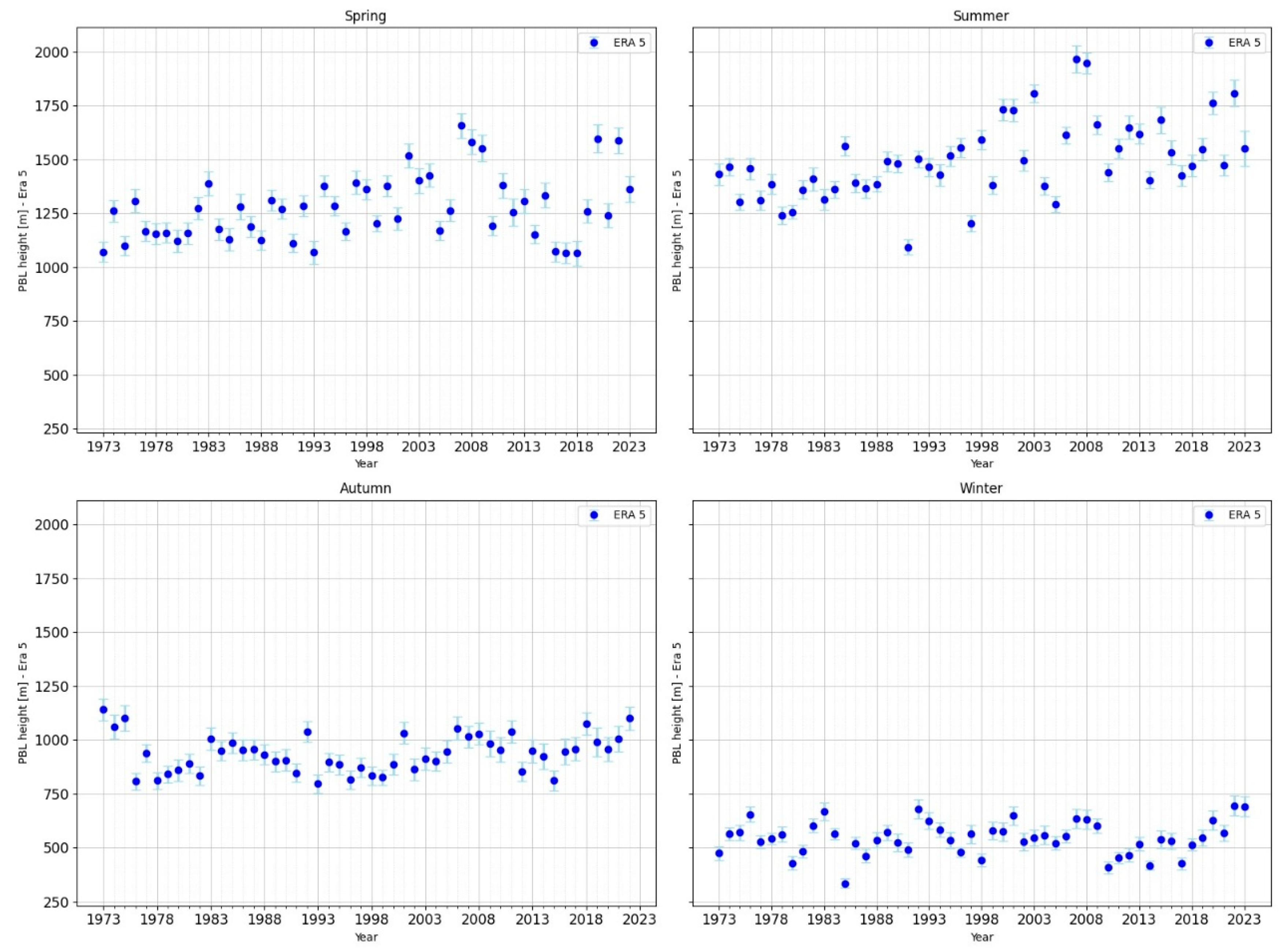
Figure 2.
Distribution of PBL height from Stull Method h12 UTC, with error bars, by seasons DJF, MAM, JJA, SON, for the period 1973-2023.
Figure 2.
Distribution of PBL height from Stull Method h12 UTC, with error bars, by seasons DJF, MAM, JJA, SON, for the period 1973-2023.
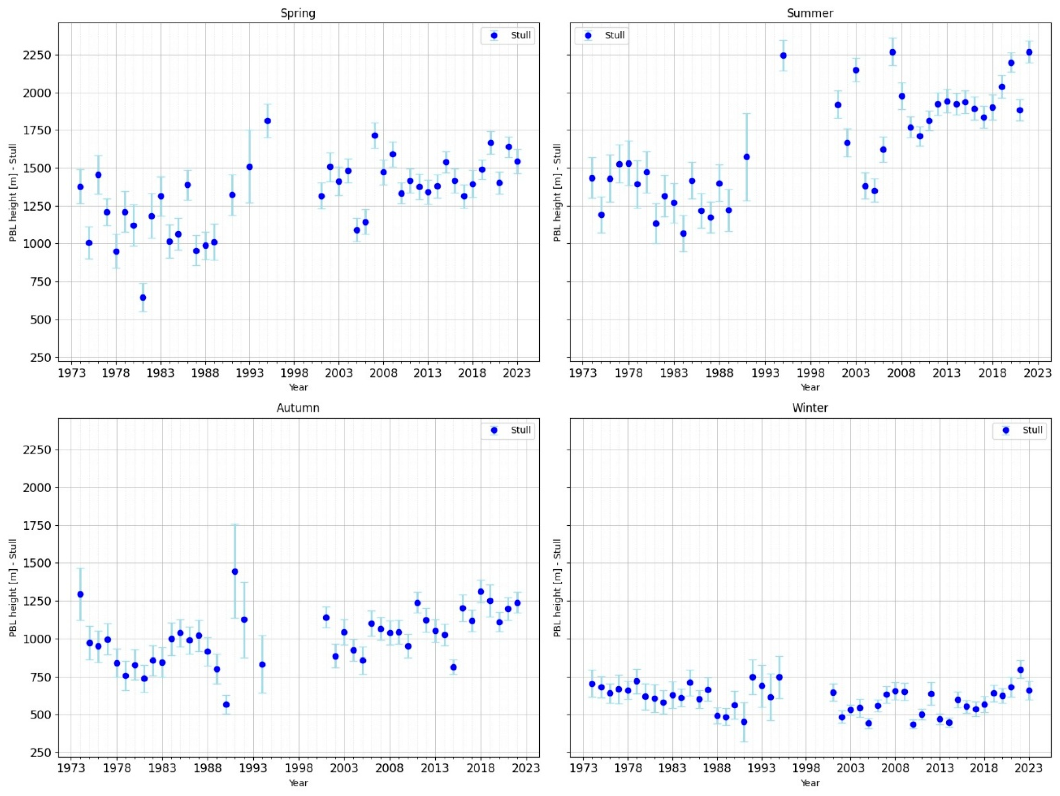
Figure 3.
Distribution of PBL height from ERA5 h00 UTC, with error bars, by seasons DJF, MAM, JJA, SON, for the period 1973-2023.
Figure 3.
Distribution of PBL height from ERA5 h00 UTC, with error bars, by seasons DJF, MAM, JJA, SON, for the period 1973-2023.
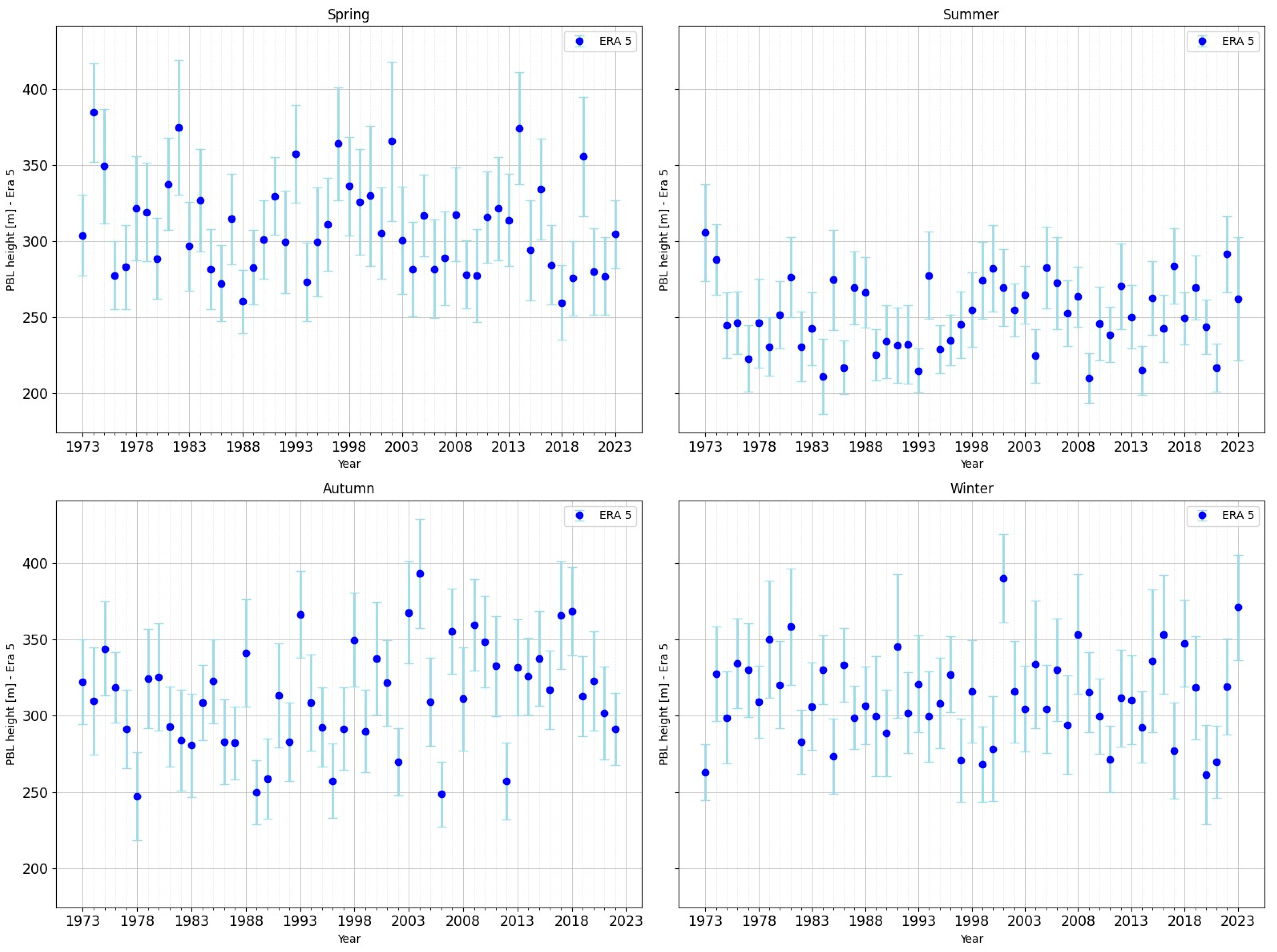
Figure 4.
Distribution of PBL height from Stull Method h12 UTC, with error bars, by seasons DJF, MAM, JJA, SON, for the period 1973-2023.
Figure 4.
Distribution of PBL height from Stull Method h12 UTC, with error bars, by seasons DJF, MAM, JJA, SON, for the period 1973-2023.
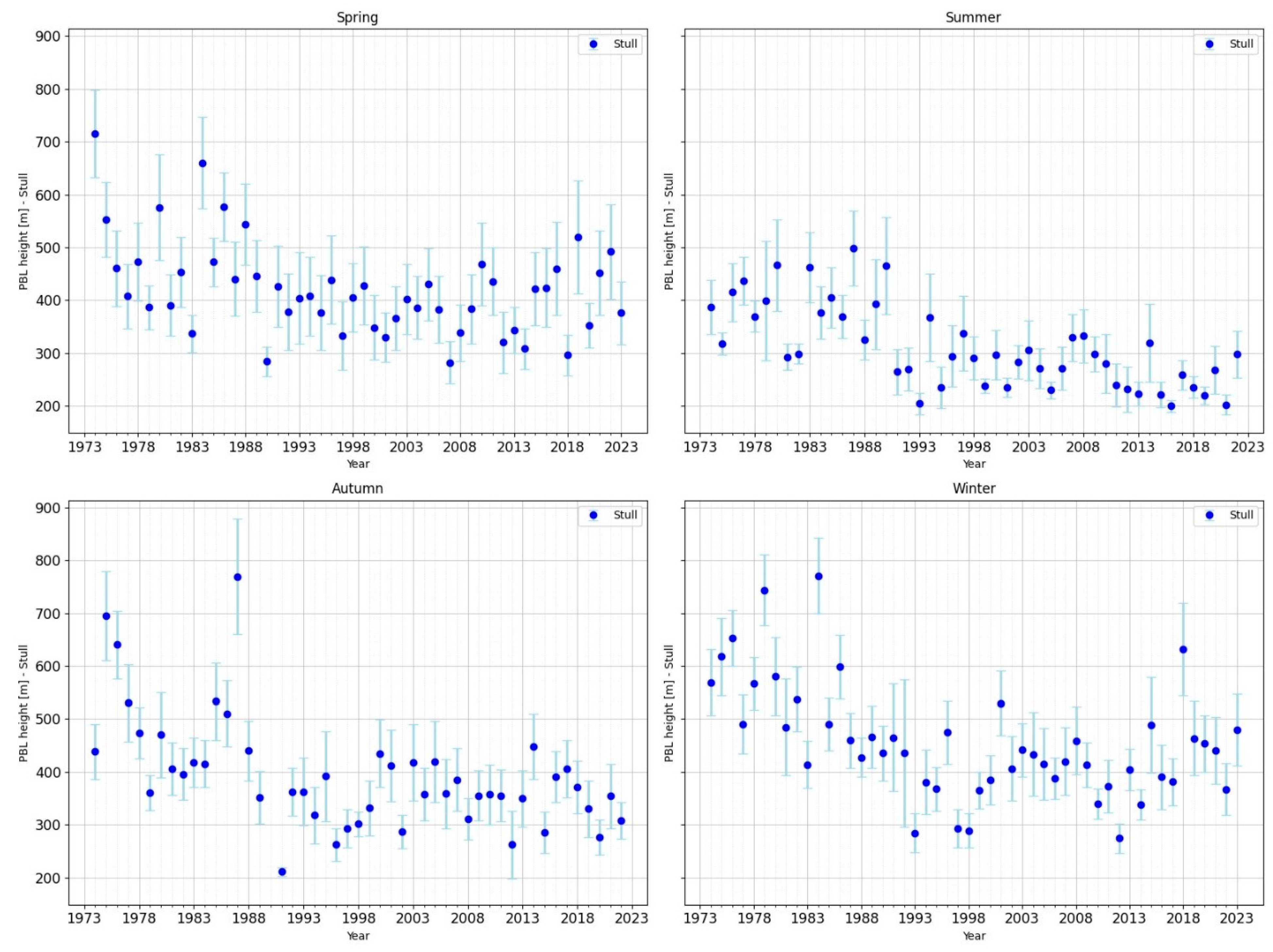
Figure 5.
Heat map for PBL height (m) average values from ERA5 at 12 UTC during the period from 1973 to 2023.
Figure 5.
Heat map for PBL height (m) average values from ERA5 at 12 UTC during the period from 1973 to 2023.
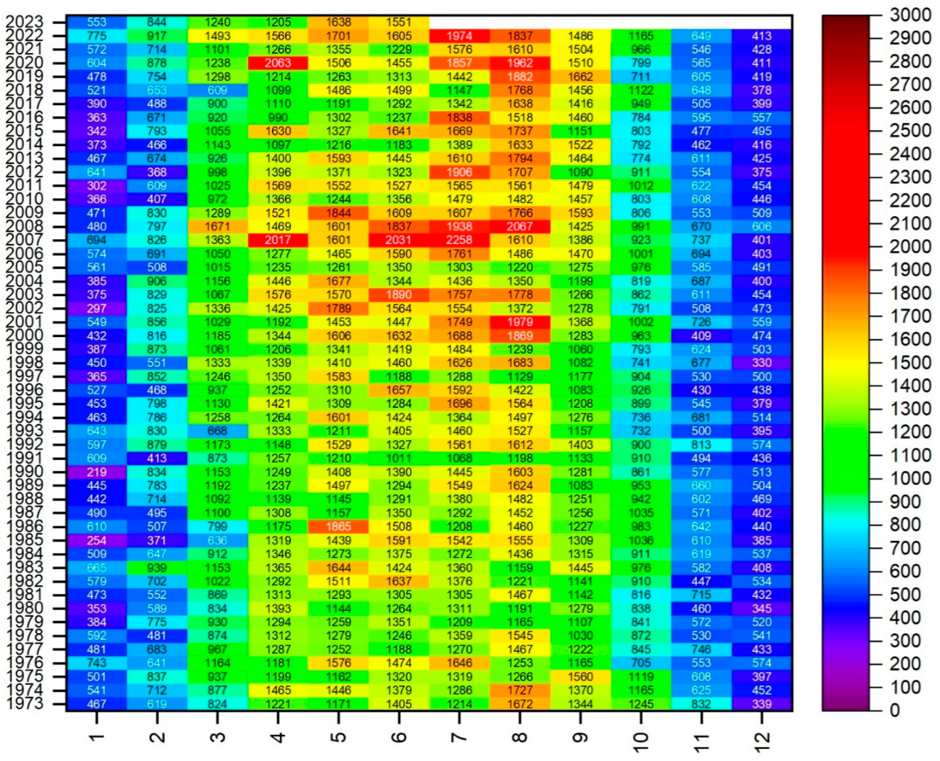
Figure 6.
Heat map for PBL height average values using the Stull method at 12 UTC during the period from 1974 to 2023.
Figure 6.
Heat map for PBL height average values using the Stull method at 12 UTC during the period from 1974 to 2023.
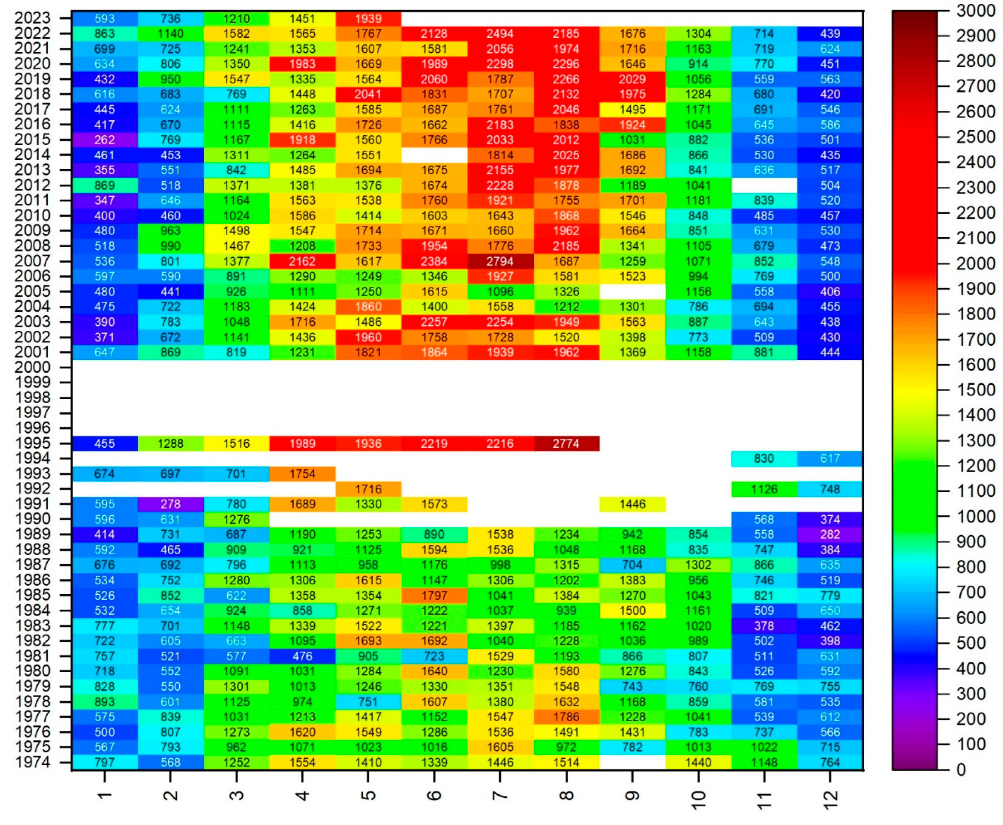
Figure 7.
Heat map for PBL height average values from ERA5 at 00 UTC during the period from 1973 to 2023.
Figure 7.
Heat map for PBL height average values from ERA5 at 00 UTC during the period from 1973 to 2023.
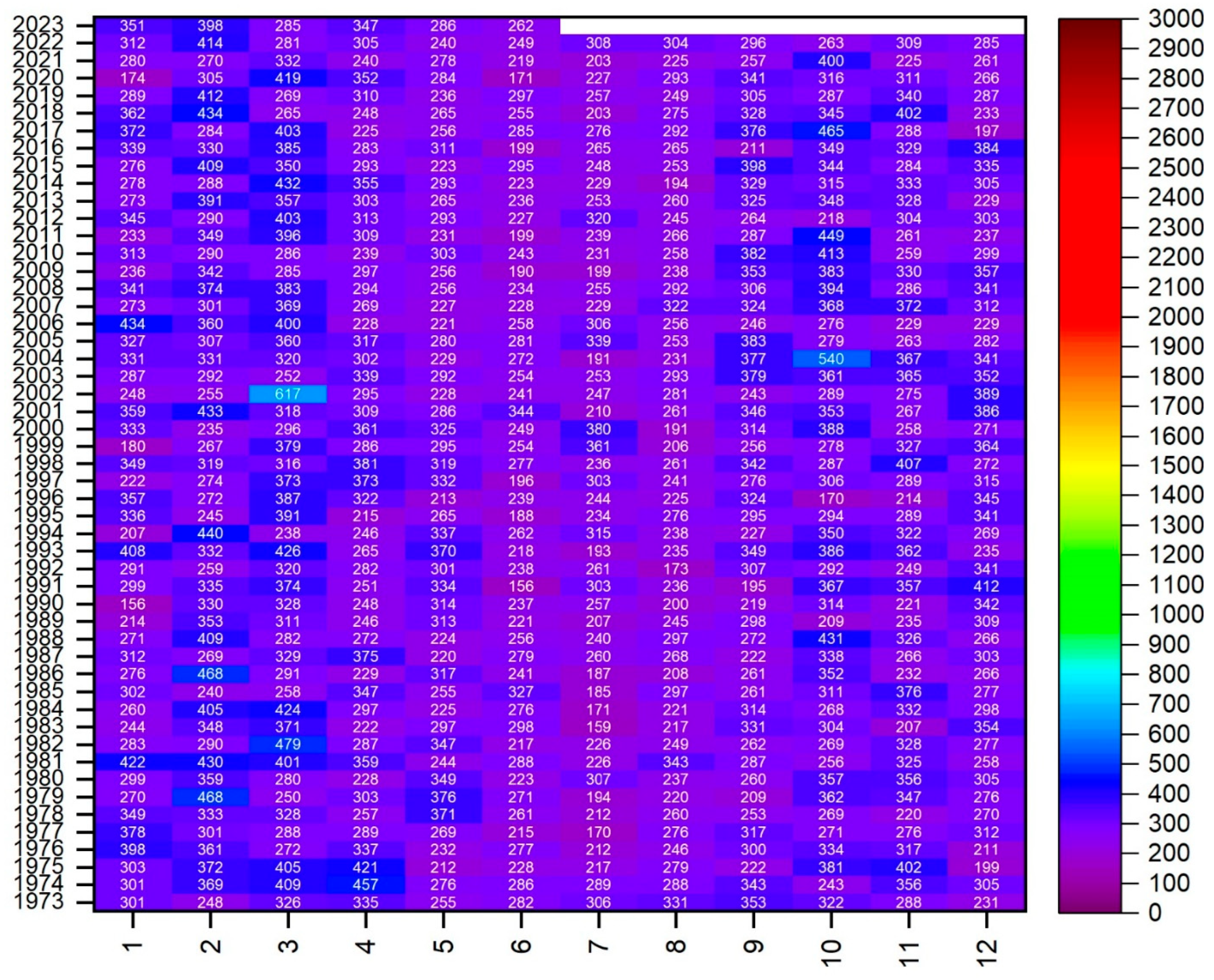
Figure 8.
Heat map for PBL height average values using the Stull method at 00 UTC during the period from 1973 to 2023.
Figure 8.
Heat map for PBL height average values using the Stull method at 00 UTC during the period from 1973 to 2023.
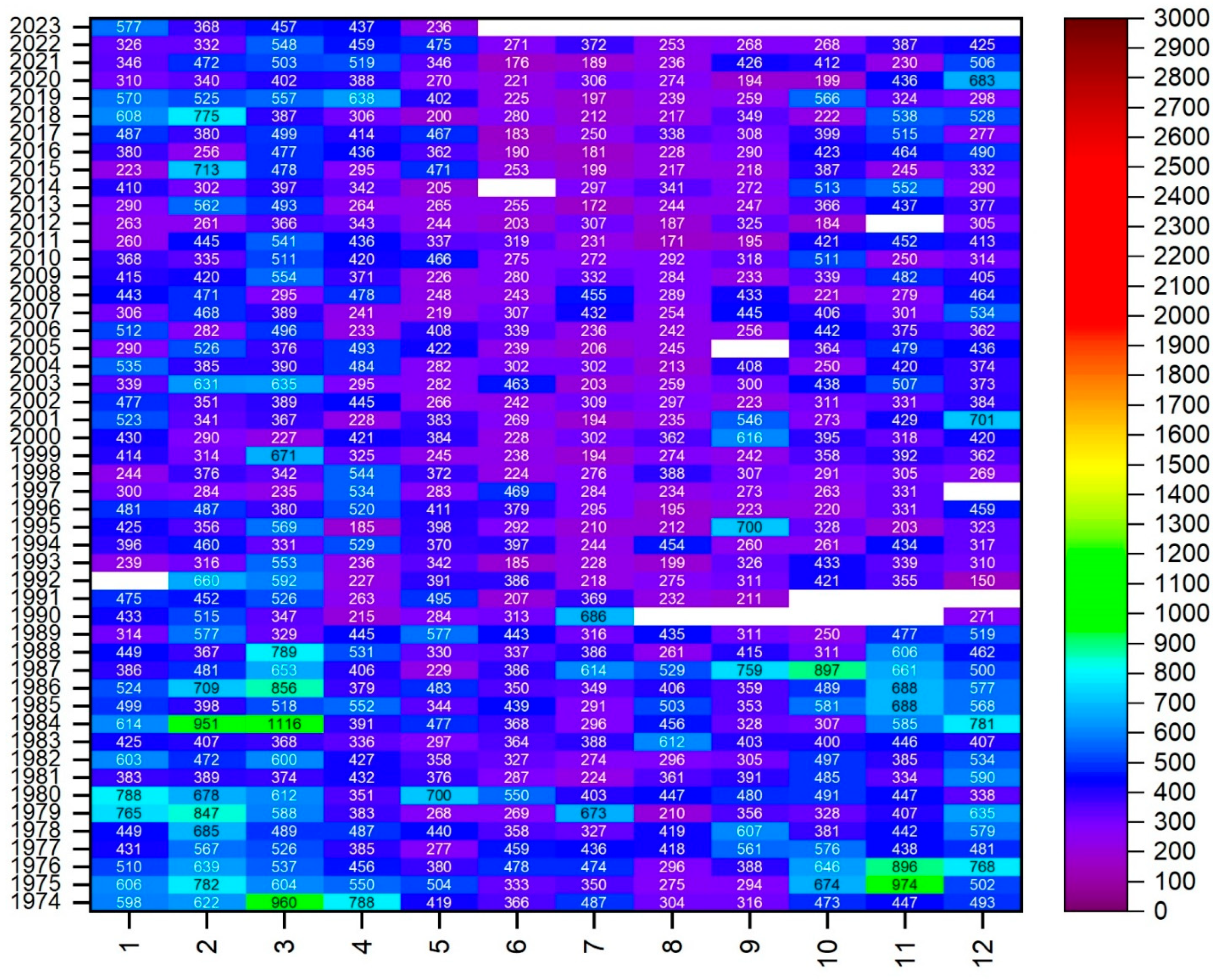

Table 1.
The minimum average values (m) of the PBL at 12 UTC determined by the Stull method and the average values of the PBL height extracted from ERA5, corresponding to the specific years of the minimum average values determined by the Stull method.
Table 1.
The minimum average values (m) of the PBL at 12 UTC determined by the Stull method and the average values of the PBL height extracted from ERA5, corresponding to the specific years of the minimum average values determined by the Stull method.
| Month | Year (specific to Stull Method) |
Minimum mean value (m) of PBL at 12 UTC from Stull Method | Mean value of PBL (m) at 12 UTC from ERA5, from the same year |
| January | 2015 | 262 | 342 |
| February | 1991 | 278 | 413 |
| March | 1981 | 577 | 869 |
| April | 1981 | 476 | 1313 |
| May | 1978 | 751 | 1279 |
| June | 1981 | 723 | 1305 |
| July | 1987 | 998 | 1292 |
| August | 1984 | 939 | 1436 |
| September | 1987 | 704 | 1256 |
| October | 1979 | 760 | 841 |
| November | 1983 | 378 | 582 |
| December | 1989 | 282 | 504 |
Table 2.
The maximum average values (m) of the PBL at 12 UTC determined by the Stull method and the average values of the PBL height extracted from ERA5, corresponding to the specific years of the minimum average values determined by the Stull method.
Table 2.
The maximum average values (m) of the PBL at 12 UTC determined by the Stull method and the average values of the PBL height extracted from ERA5, corresponding to the specific years of the minimum average values determined by the Stull method.
| Month | Year (specific to Stull Method) |
Maximum mean value (m) of PBL at 12 UTC from Stull Method | Mean value of PBL (m) at 12 UTC from ERA5, from the same year |
| January | 1978 | 893 | 592 |
| February | 1995 | 1288 | 798 |
| March | 2022 | 1582 | 1493 |
| April | 2007 | 2162 | 2017 |
| May | 2018 | 2041 | 1486 |
| June | 2007 | 2384 | 2031 |
| July | 2007 | 2794 | 2258 |
| August | 1995 | 2774 | 1564 |
| September | 2019 | 2029 | 1662 |
| October | 1974 | 1440 | 1165 |
| November | 1974 | 1148 | 625 |
| December | 1985 | 779 | 385 |
Table 3.
The minimum average values (m) of the SBL at 00 UTC determined by the Stull method and the average values of the PBL height extracted from ERA5, corresponding to the specific years of the minimum average values determined by the Stull method.
Table 3.
The minimum average values (m) of the SBL at 00 UTC determined by the Stull method and the average values of the PBL height extracted from ERA5, corresponding to the specific years of the minimum average values determined by the Stull method.
| Month | Year (specific to Stull Method) |
Minimum mean value (m) of PBL at 00 UTC from Stull Method | Mean value of PBL (m) at 00 UTC from ERA5, from the same year |
| January | 2015 | 223 | 276 |
| February | 2016 | 256 | 330 |
| March | 2000 | 227 | 296 |
| April | 1995 | 185 | 215 |
| May | 2018 | 200 | 265 |
| June | 2021 | 176 | 203 |
| July | 2013 | 172 | 253 |
| August | 2011 | 171 | 266 |
| September | 2020 | 194 | 341 |
| October | 2012 | 184 | 218 |
| November | 1995 | 203 | 289 |
| December | 1992 | 150 | 341 |
Table 4.
The maximum average values (m) of the SBL at 00 UTC determined by the Stull method and the average values of the PBL height extracted from ERA5, corresponding to the specific years of the minimum average values determined by the Stull method.
Table 4.
The maximum average values (m) of the SBL at 00 UTC determined by the Stull method and the average values of the PBL height extracted from ERA5, corresponding to the specific years of the minimum average values determined by the Stull method.
| Month | Year (specific to Stull Method) |
Maximum mean value (m) of PBL at 00 UTC from Stull Method | Mean value of PBL (m) at 00 UTC from ERA5, from the same year |
| January | 1980 | 788 | 299 |
| February | 1984 | 851 | 405 |
| March | 1984 | 1116 | 424 |
| April | 1974 | 788 | 457 |
| May | 1980 | 700 | 349 |
| June | 1980 | 550 | 223 |
| July | 1990 | 686 | 257 |
| August | 1983 | 612 | 217 |
| September | 1987 | 759 | 222 |
| October | 1987 | 897 | 338 |
| November | 1975 | 974 | 402 |
| December | 1984 | 781 | 298 |
Disclaimer/Publisher’s Note: The statements, opinions and data contained in all publications are solely those of the individual author(s) and contributor(s) and not of MDPI and/or the editor(s). MDPI and/or the editor(s) disclaim responsibility for any injury to people or property resulting from any ideas, methods, instructions or products referred to in the content. |
© 2025 by the authors. Licensee MDPI, Basel, Switzerland. This article is an open access article distributed under the terms and conditions of the Creative Commons Attribution (CC BY) license (http://creativecommons.org/licenses/by/4.0/).
Copyright: This open access article is published under a Creative Commons CC BY 4.0 license, which permit the free download, distribution, and reuse, provided that the author and preprint are cited in any reuse.


