Submitted:
01 October 2025
Posted:
02 October 2025
You are already at the latest version
Abstract
Simulation of damage scenarios is an important tool for seismic risk mitigation. While a detailed analysis of each building would be preferable to assess their vulnerability to seismic hazard, at large urban scale simplified yet robust methodologies are necessary to overcome computational costs or data unavailability. Moreover, most damage assessments simulate single seismic shocks, though in many real sequences, with a series of aftershocks following the mainshocks, it is observed that buildings endure damage accumulation, which increases their vulnerability over time. The present study builds on a recently developed methodology for simulating urban-scale damage scenarios across seismic sequences, explicitly accounting for damage accumulation and the evolution of vulnerability. In particular, the availability of a dataset reporting the damage observed in the L’Aquila area (Italy) during the severe earthquake sequence of 2009, in combination with the georeferenced maps representing the spatial distribution of the ground motion, allows for the calibration of the methodology through the comparison between the simulations’ results and the sequence’s real data. Although calibrated on the L’Aquila dataset, the proposed procedure could also be applied to different urban areas, with both real and synthetic seismic sequences, enabling the forecasting of damage scenarios to support the development of effective strategies for seismic risk mitigation.
Keywords:
damage forecast
; seismic vulnerability
; urban areas
1. Introduction
As urban areas become increasingly vulnerable to seismic hazards with ageing infrastructure on one hand and rapid urbanisation on the other, forecasting earthquake-induced damage is essential for risk mitigation and emergency planning. Detailed modelling of individual buildings is often computationally challenging; for this reason, simplified yet robust methodologies have been developed to capture key aspects of structural vulnerability [1,2,3]. At large urban scale, evaluating a significant number of buildings is impractical and requires efficient methods that balance accuracy and speed. Furthermore, reliable data on the construction materials, structural design, and condition of each building is often lacking or difficult to obtain, especially in older cities.
Among the most widely used approaches is Rapid Visual Screening (RVS) [4], which relies on visual inspections to estimate vulnerability based on external characteristics. More advanced methodologies, which also have been applied to seven European cities in the context of the RISK-EU project [5], include Vulnerability Index Methods (VIM), which assign numerical vulnerability scores based on structural features and historical damage data, and the Macroseismic approach [6], which relates vulnerability indices to expected damage at given intensities using analytical functions (vulnerability curves) derived from the European Macroseismic Scale EMS-98 [7]. Damage Probability Matrices (DPMs) and fragility functions are two commonly used tools for assessing the likelihood of structural damage under seismic action. DPMs provide the probability of a structure being in each predefined damage state at specific intensity levels, typically in a discrete, tabular format [8,9,10]. Fragility functions express the probability of exceeding a given damage state as a continuous function of seismic intensity, capturing uncertainty in structural response. While DPMs are often derived from empirical observations or expert judgment, fragility functions are usually developed through analytical modelling or statistical analysis of observed damage data [11,12]. In recent years, Machine Learning Algorithms (MLA) have also been introduced as they process large datasets and identify patterns across building typologies, helping to automate the vulnerability estimation process, particularly when detailed structural information is unavailable [13]. Seismic damage scenario simulation can be performed using a variety of tools and methodologies that combine hazard information, building vulnerability models, and exposure data. Among these tools, one widely used is OpenQuake [14], developed by the Global Earthquake Model Foundation (GEM), that offers a global, open-source computational engine, which has been employed, for example, in the Italian Risk Maps platform (IRMA) [15]. While these methods provide standardized and computationally efficient frameworks, they typically focus on a single event scenario or on Probabilistic Seismic Hazard Assessment (PSHA), overlooking the cumulative effects of earthquake sequences, where foreshocks and aftershocks can progressively weaken structures over time, increasing their vulnerability. Recent advances in Performance-Based Earthquake Engineering (PBEE) have highlighted the importance of accounting for sequential seismic loading, for example by incorporating state-dependent fragility functions in a Markovian framework to capture damage cumulation over multiple mainshock–aftershock events, addressing limitations of traditional single-event probabilistic seismic risk models [16]. In this context, the 2009 earthquake sequence in the L’Aquila region of central Italy presents a valuable opportunity for methodological development and empirical validation. The sequence, which included a destructive mainshock and several significant aftershocks, caused widespread damage across the urban area, which has been documented and collected in the Database of the Observed Damage Da.D.O. (“Database del Danno Osservato” in Italian) developed by the Eucentre Foundation [17,18].
In this paper we follow an innovative approach for simulating seismic damage accumulation at the urban scale proposed in recent studies by some of the present authors and focused on the numerical simulation of earthquake sequences [19,20]. The insights and innovations compared to the previous models are multiple and mainly include the adoption of a real seismic sequence (instead of an artificial one) and of a real damage dataset (not available in preceding studies). In particular, we consider as a case study the area affected by the 2009 L’Aquila sequence, and our main goal is to simulate, by reproducing the sequence of earthquakes that occurred during the period of most intense seismic activity, the damage caused to the buildings in the considered area. This sequence is reconstructed using the ShakeMaps, georeferenced maps representing the spatial distribution of the ground motion, generated by the Italian National Institute of Geophysics and Volcanology (INGV) for the corresponding seismic events [21,22,23]. The simulated damage is then compared with the actual damage data reported in the Da.D.O., which includes a comprehensive record of 74,049 buildings in proximity of L’Aquila. The comparison with the observed data will allow us to calibrate the simulation methodology in order to provide more accurate and reliable results. Once successfully calibrated on the L’Aquila data, this method could be extended and applied to other seismic active areas for both real and artificial seismic sequences. It can significantly aid in developing effective risk management strategies, particularly when supplemented with additional data on road infrastructure, if available [24]. This paper is structured as follows: firstly, it introduces the L’Aquila case study and the datasets used for calibration; secondly, it details the methodological framework for modelling damage accumulation and vulnerability update; finally, it presents and discusses the results of the simulations and their implications for urban seismic risk mitigation.
2. The Case Study of L’Aquila
In 2009 the Abruzzo region in central Italy experienced a prolonged sequence of seismic events. The sequence began in December 2008 and culminated on April 6, 2009, with a major earthquake of moment magnitude Mw 6.1, occurring at 3:32 AM local time. The mainshock, followed by numerous aftershocks, had its epicenter near the city of L’Aquila, the capital of the Abruzzo region. The earthquake’s shallow depth of approximately 8.8 kilometers significantly contributed to the extensive damage observed in the area. The QUick Earthquake Survey Team (QUEST) was mobilized immediately after the mainshock to conduct the macroseismic survey on the affected localities [25]. According to the authors of the report, the assessment was challenging due to the high variability of the constructions’ typology and state of maintenance, especially between historical centres and suburban areas. The observed damage spatial distribution reflected the location and orientation of the seismogenetic source (a 40 km long NW-SE trending normal faults system) [26,27], although intensity anomalies were observed due to local site effects and topography influence. The resulting report in Mercalli-Cancani-Sieberg scale (MCS) [28] is said to reflect mainly the mainshock and its effect on the historical centres of the localities. However, the survey has been conducted from the 6th of April to the 1st of July, involving 316 localities, with several requiring a re-evaluation, and some being revised according to the EMS-98. The L’Aquila 2009 sequence provided an ideal case study for the application and validation of the U.S. Geological Society (USGS) software ShakeMap [21], which had recently been adapted for Italy by the INGV [22]. In the INGV ShakeMap application to L’Aquila, the resulting instrumental MCS intensity ShakeMap was compared with the MCS intensity values reported by the QUEST, showing qualitative similarity and highlighting the accuracy of the instrumental intensity estimates [29]. Moreover, the Italian Department of Civil Protection (DPC) led an extensive post-earthquake damage survey campaign to gather data on the buildings affected by the event. The collected information was later conveyed in the Da.D.O. [17,18], together with other relevant Italian post-earthquake campaigns, providing an invaluable resource for studies on seismic damage and building vulnerability.
In this study, we exploit the instrumentally derived intensity maps provided by the INGV and the L’Aquila 2009 dataset from Da.D.O. to test, through extensive numerical simulations, some hypothesis of damage accumulation and to compare the simulation results with the observed damage scenario.
2.1. The Seismic Input: INGV Instrumental Intensity ShakeMaps
In Italy, the INGV ShakeMap implementation rapidly generates the spatial distribution of ground motion parameters after each seismic event of moment magnitude (Mw) greater than 3.0. The software interpolates ground shaking measurements recorded at seismic stations with seismological data on the event (epicentral coordinates, moment magnitude, depth) and on the seismic source (style of faulting) through models that predict ground motion (Ground Motion Prediction Equation, GMPE) based on seismic wave propagation, and also accounting for geological site effects. The resulting maps are available in terms of Peak Ground Acceleration (PGA), Peak Ground Velocity (PGV), Spectral Acceleration (SA) at three periods, and intensity. The latter is derived instrumentally by applying Ground Motion to Intensity Conversion Equations (GMICEs), or IPEs (Intensity Prediction Equations) when data is limited. The INGV ShakeMap initial implementation employed regional GMPEs derived for the Italian territory earthquakes of magnitude < Mw 5.5, while equations developed more broadly for the European context were used for events of greater magnitudes ([22] and reference therein). A following update of the software introduced a new GMICE [30], hereinafter “FM10”. The current INGV ShakeMap implementation [23] selects the best performing ground motion model based on seismotectonic zonation (e.g., Bindi et al. [31], hereinafter “ITA10”, for areas such as the L’Aquila 2009 territory). Most recently, since March 2023, the GMICE by Oliveti et al. [32] has replaced the previous GMICE. The new model, regressed on a more comprehensive dataset [33], demonstrated greater accuracy and improved predictive performance, addressing the limitations of the FM10 GMICE, which slightly overestimate the intensity for earthquakes of magnitude greater than Mw 5.0. The seismic sequence selected as case study in this paper occurred prior to the most recent update of the GMICE. Consequently, the associated ShakeMaps in the INGV ShakeMap Archive (https://shakemap.ingv.it/archive.html, last accessed March 2025) were generated using the ITA10 GMPE, and the FM10 GMICE, according to the metadata of the downloadable products available on the cited website.
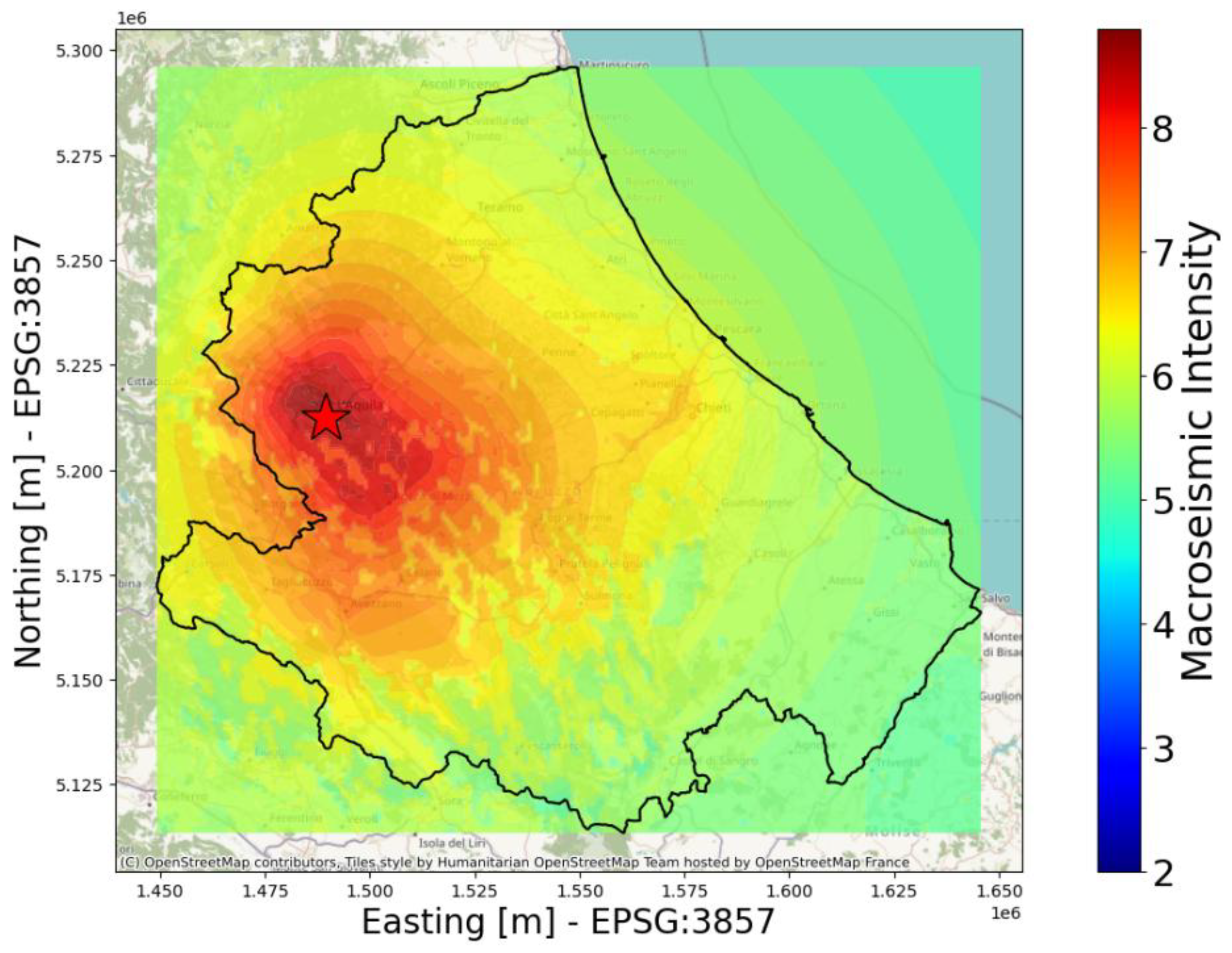
Figure 1.
Macroseismic intensity ShakeMap generated by the INGV for the L’Aquila 2009 mainshock (available on the INGV ShakeMap Archive, https://shakemap.ingv.it).
Figure 1.
Macroseismic intensity ShakeMap generated by the INGV for the L’Aquila 2009 mainshock (available on the INGV ShakeMap Archive, https://shakemap.ingv.it).
We selected two possible configurations of seismic input for damage assessment: either considering only the Mw 6.1 mainshock or including all the earthquakes of magnitude greater than Mw 4.0, from the mainshock of the 6th of April 2009 to the last Mw 5.0 event on the 9th of April 2009. The earthquakes of the considered sequence are characterized by the following parameters: date, UTC time, epicentral coordinates, depth and moment magnitude, all included in the array Qi = {Ei, Di, Ti, Lati, Loni, Dei, Mwi}, i=1,…,18 (see Table 1). Figure 2 shows the moment magnitudes of the 18 earthquakes selected from the L’Aquila 2009 sequence in chronological order.
2.2. The Da.D.O. Buildings Dataset
In this paper we utilize the extensive Da.D.O. dataset [17,18], which includes detailed records of 74,049 buildings located near L’Aquila. It provides pre-event characteristics such as the buildings’ age, construction materials, and geometry, along with post-event damage evaluations conducted after the five most significant earthquakes, each exceeding a magnitude of Mw 5.0, which occurred between April 6 and April 9, 2009. The data are accessible by authorized researchers through a WebGIS platform developed by the Eucentre Foundation. In Figure 3, panel (b), the epicenters of these earthquakes are indicated by red star symbols, with the main event of magnitude Mw 6.1 additionally marked by a yellow circle. The spatial distribution of the buildings in the dataset is illustrated in panel (c) of the same figure, showing their geographical locations within the impacted area.
The 74,049 buildings of the original Da.D.O. dataset can be classified according to their construction types, which include Masonry, Reinforced Concrete (RC), Mixed and Steel. Figure 4 illustrates the composition of the dataset, reporting the corresponding percentages of each class.
As further specified in Figure 5, more than half of the masonry buildings considered were constructed before 1919. This distribution reflects historical construction trends in Italy, where unreinforced masonry was the predominant structural system until the early 20th century. Starting from the 1970s, a significant shift occurred, following the progressive development of seismic design codes and the growing adoption of reinforced concrete systems [34]. This led to a steady decline in the use of masonry for new constructions. The Abruzzo region had already been severely affected by a major seismic event in 1915, known as the Marsica earthquake, which caused widespread destruction and over 30,000 casualties. In response, the Royal Decree n. 573 of 29 April 1915, was issued, marking one of the first attempts to introduce seismic zoning in Italy, with the classification of several municipalities, including those in Abruzzo, as seismic zones. From the 1970s onwards, increased attention was paid to the quality of masonry construction, as shown in Figure 5b. This was partly due to the introduction of the Italian Law n. 64 of 2 February 1974 and subsequent technical standards, which provided measures for structures, with particular emphasis on those in seismic areas. These regulations significantly contributed to the modernization of construction practices, including stricter requirements for materials, detailing, and structural analysis. They led to improvements not only in vertical load-bearing walls, but also in the design of horizontal diaphragms and in the presence of chains or curbs, as shown in Figure 5. Beginning from that period, traditional vaulted systems and flexible timber slabs (see Figure 6 (a) and (b), which exhibit poor in-plane stiffness, began to be progressively replaced by reinforced concrete beams and semi-rigid or rigid slabs (see Figure 6 (c)). This shift resulted in improved in-plane stiffness and a more effective transfer of seismic forces between structural elements.
A preliminary statistical overview of the dataset under analysis reveals that it is composed of masonry buildings with a low to medium height profile, typically ranging from 1 to 4 storeys. The interstorey height is concentrated in the 2.50–3.50 m interval, and the floor area is mostly under than 100 m2. These distributions, shown in Figure 7, are representative of the predominant typologies of buildings in the studied region, characterized by compact footprints and modest vertical development.
In this paper, we focus exclusively on masonry buildings for the following reasons: (1) they constitute the highest percentage of the dataset; (2) they experienced the most severe levels of damage but, at the same time, (3) a significant percentage of them remained lightly damaged or undamaged; (4) the macroseismic survey is mostly representative of the historic city centers, where the masonry buildings are predominant; and, finally, (5) the fragility model utilized in this analysis has been developed specifically for masonry structures (see Paragraph 3.). We applied standard preprocessing to the initial dataset to exclude entries with missing information on location, observed damage, and vulnerability classification. The final operative dataset used in the simulations consists therefore of 47,049 masonry buildings.
2.3. Initial Vulnerability Class and Observed Damage in the Da.D.O. Dataset
The information contained in the Da.D.O. dataset includes building identification, building description (number of floors, age, purpose of use, etc.), types of vertical and horizontal structures, damage to structural and non-structural elements, external danger induced by other constructions and morphology of the site.
Using this information, an initial vulnerability score can be determined for each building. This score is categorical, ranging from level A (indicating the highest vulnerability) to level D2 (indicating the lowest vulnerability)1. For masonry buildings the vulnerability class based on the quality of the vertical structure, the horizontal structure and the presence of chains (see Table 2) is assigned. Therefore, the resulting vulnerability classification for masonry buildings ranges from A to C1. The buildings realized after the seismic Italian Law should be associated with D1 class, but they are very few and are therefore classified as C1 class. For other typologies of construction, not considered here, a different method is adopted: reinforced concrete structures are assigned either in class C2 or D2 based on the year of construction with respect to the year of seismic classification of the municipality; steel and mixed buildings are assigned to D2 and C2 respectively.
In the numerical simulations, the vulnerability class of each building was iteratively updated based on the damage caused by the seismic ground motion intensity. The observed damage data served as the target reference for evaluating the simulation results. The four potential issues described in the following should be addressed when working with the Da.D.O. dataset for L’Aquila 2009 buildings. First, while the buildings are categorized into vulnerability classes based on a limited number of structural features, alternative methods consider additional factors such as maintenance level, position, resonance effects and topography. This raises the concern that the assigned vulnerability classes may not fully represent the true vulnerability of the building and, consequently, the observed damage. Second, as already analysed in [11], the L’Aquila 2009 dataset together with the Irpinia 1980 dataset are the only dataset in Da.D.O. that have the highest completeness ratio of 90%, which is the fraction of buildings surveyed during damage assessment campaigns compared to the total number of buildings reported by national census (for L’Aquila 2009, the reference census is the ISTAT 2001). However, some buildings in the dataset were completely surveyed, while others were assessed only partially or externally. This discrepancy is accounted for in [35], where different weights are applied to the damage on structural elements based on the level of assessment. Third, according to the authors of the Da.D.O., the buildings were semi-automatically georeferenced by means of a tool developed by the Eucentre, with a reported error of 5-10% of buildings located at the barycentre of the municipality. However, we noted that some buildings are also located at the centroid of the locality, a smaller administrative boundary in Italy. For example, in the municipality of Campotosto, a cluster of building is positioned at the centroid of the municipality, which unfortunately is localized in lake of Campotosto. Another cluster can be found at the centroid of a locality of Campostosto. These georeferencing errors could represent an issue when associating the building to the intensity value from the ShakeMap, as the Vs30 value or the epicentral distance might differ from the actual position and the centroid. Finally, the source of the observed damage data in Da.D.O. is the AeDES (“Agibilità e Danno nell’Emergenza Sismica” in Italian) form [36,37], which has been used as the operational inspection tool for surveys after seismic emergency since 1997, as defined by the DPC2. This tool assesses the damage by evaluating the structural elements, assigning them one of four damage levels: D0 (“no damage”), D1 (“light damage”), D2/D3 (“moderate/severe damage”), D4/D5 (“extremely severe damage”). Additionally, to quantify the extension of the damage, a value is assigned ranging from less than 1/3, to between 1/3 and 2/3, or greater than 2/3. In Da.D.O., an observed damage grade ) associated only to the vertical structure of the building is assigned. This damage grade is derived by employing a conversion table that translates the damage levels and extensions from the AeDES form into the six levels of the EMS-98 from D0 to D5. A global damage level is here evaluated by means of the expression provided in [35], which weights the damage at the different structural elements based on the extension and damage level:
where the weights for a given structural element, as anticipated, differ whether the survey was complete or partial; are the percentages of a structural element i (where i=1,..,5 corresponding to vertical structures, horizontal structures, stairs, roof, infills) in which the damage j was observed (where j=1,…,3 correspond to the AeDES damage levels D1, D2/D3, D4/D5). For detailed information regarding the formula and the values of the weights, please refer to the original article [35]. In Figure 8, for each vulnerability class, we compare the difference between the damage levels observed according to Da.D.O. method ) and to Equation (1) . The damage distribution, representing a comprehensive elaboration of the observed damage, was used as a benchmark to assess the consistency of the simulated damage results.
3. Simulation of Damage Evolution
As anticipated in the Introduction, in this paper we followed an approach proposed in recent studies [19,20], focused on the simulation of earthquake sequences in large urban areas and on the evaluation of the consequent seismic damage accumulation on buildings. The original approach was based on an agent-based model which allows to simulate an artificial seismic sequence using an opportune version of the Olami-Feder-Christensen (OFC) model [38,39] and to assess the resulting damage on an urban setting through a given fragility model, updating the vulnerability of the buildings and accumulating the damage after each event of the synthetic sequence. Differently, in this study we incorporated data from real recorded seismic sequences and from observed damage datasets in order to evaluate the effects of different seismic inputs (either a single event or a sequence), in terms of fragility models, damage accumulation and vulnerability evolution functions on damage scenarios simulations.
One of the main reasons for further developing the previous approach was the possibility to use the data from the Da.D.O. dataset, which allowed a more accurate calibration. To this aim, the OFC-based synthetic sequence was replaced with data from actual registered seismic sequences. Given a list of georeferenced earthquakes as detailed in Paragraph 2.1, to each building was assigned an intensity value I from the corresponding available macroseismic intensity ShakeMap generated by the INGV. After the first shock, the most probable value of expected damage was assigned to each building based on a fragility model. In this study, we adopted the model developed by Lagomarsino, Cattari and Ottonelli (2021) [35], hereinafter “L21”, which derived its methodology from the macroseismic model by Lagomarsino and Giovinazzi (2006) [6] (“L06”) but was recalibrated on the Da.D.O. datasets. This calibration aimed at improving the regression of the vulnerability curves, which express the mean expected damage on each building as a function of the intensity I of the earthquake and of the building’s vulnerability V:
In this paper, is the instrumental intensity from the ShakeMap, which, as already detailed, was derived from recorded PGM and from ground motion models that take into account the amplification value of the soil below the building. Each building was initially assumed to be in un undamaged state, namely D0, and it was assigned a starting vulnerability value , randomly selected within the plausible range corresponding to its vulnerability class, as defined by the fragility model (Table 3). It must be noted that the L21 model consider the standard EMS-98 classification of vulnerability from A to F. Since this study focuses on masonry buildings, only classes A, B and C1 were considered; with class C1 values adapted as the upper interval of class C. In order to consider the damage cumulative process related to repetitive events, a possible choice was the simple original strategy proposed by Greco et al. (2019) [19] for evaluating the reduction of structural performance associated to a sequence of earthquakes. After each earthquake i, the mean damage level was computed according to the vulnerability model (Eq. (2)), as a function of the seismic intensity felt at the building’s site and of the vulnerability of the building, that is the updated vulnerability after the previous event. The building’s damage level was then evaluated as the most probable mean damage level . Then, the total damage level for each building is defined as the sum of the damage levels for each previous seismic event. After being damaged, the building increases its vulnerability to assumed to follow an update rule.
In this paper we propose a new vulnerability update rule , Eq. (3), based on the following constraints: (a) the initial vulnerability is assumed to vary from 0 to 1 or slightly exceeds this range, as it shown in the plausible ranges in Table 3; (b) to employ the fragility models, the vulnerability index is required to vary in those ranges; (c) the EMS-98 states that during a sequence, the vulnerability of an already damaged building might differ from its initial vulnerability; (d) however there is no data on how far could those intervals be extended or shifted for the vulnerability of a damaged building; (e) Grimaz and Molisan (2017) [40] have proposed the definition of an higher vulnerability class A- that would characterize buildings that have experienced a damage grade ≥ D3 prior to the new shock. We have therefore tried to develop a vulnerability update rule that would increase more rapidly if a building has suffered a damage level equal or greater than D3 after the previous event, and so that the updated vulnerability reaches its maximum as the upper bound of the plausible range for a new class of vulnerability A-, as defined in Table 4.
In this case the vulnerability increases with the damage following an exponential curve, as shown in Figure 9. Again, subsequent earthquakes can progressively injure both already damaged and undamaged buildings, increasing their Total Damage Level . After the last event of the sequence, the final total damage level assigned to each building is converted into a categorical value, from D0 to D5.
4. Results
In this section we apply the model to the data to address two main seismic scenarios: a mainshock- only scenario and a whole-sequence scenario.
To compare the simulation results with the observed data, the percentage distribution of buildings per vulnerability class across damage levels was computed and, both qualitatively and quantitively, compared to the observed one, by calculating the Root Mean Square Error (RMSE) as:
where and are respectively the observed and simulated frequencies for each final damage level, from D0 to D5.
For a given model configuration, multiple simulation runs were performed and the final damage distributions were averaged in order to obtain more reliable statistics. To assess how many runs are needed to stabilize the averaged quantities, we decided to produce N=100 different realizations. To evaluate the stability of the simulation results, the mean damage level calculated over all the buildings at the end of each realization was computed, by translating its D0-D5 categorical value into an integer value included in the range [0, 5]. This value has been further averaged over the previous realizations and plotted as function of the number of runs, together with its corresponding standard deviation. The stability results will be shown for each seismic scenario.
4.1. Mainshock-Only Scenario
In the mainshock-only scenario, the damage tends to be overestimated, likely as a result of the overprediction of the intensity values. In Figure 10 are shown the results of the damage distribution after the main event of Mw 6.1, considering all the masonry buildings present in the L’Aquila 2009 Da.D.O. dataset. Looking at the percentages of buildings presenting a given final simulated damage for each initial vulnerability class, it clearly appears that these percentages are significantly overestimated (in particular for intermediate levels of damage) when compared to the observed distribution.
To address this issue and account for the potential influence of additional factors not explicitly included in the model, a certain amount of randomness was incorporated into the analysis. This was achieved by assigning to each building an initial random vulnerability value, within the range specified by its vulnerability class. Furthermore, for each seismic event, the number of buildings subjected to damage accumulation was randomly sampled using a control parameter P, which corresponds to the percentage of buildings located within each ShakeMap polygon (see Figure 1). We stress that each polygon is characterized by a unique value of the intensity.
Varying the P parameter and calculating for each value of P the root mean squared error RMSE associated between the simulated and observed damage distributions, we found that the minimum RMSE is observed at P=40% (Figure 11).
The distribution associated with P=40% is shown in Figure 12. The fragility model appears to fail to populate the highest damage grades, leaving room for testing the hypothesis of damage accumulation when applying them to the whole sequence.
As anticipated, a stability analysis was performed on the simulations. The results in Figure 13 show the stability plot for the mainshock-only scenario simulated for P=40% and using L21 as the fragility model. The average value quickly converges to around 1.693 and remains constant, with its standard deviation, after approximately 30 simulation runs. This indicates that the simulation produces consistent and reliable results already beyond this threshold. However, as expected, the mean simulated value overestimates the observed mean final damage (0.799), indicating potential systematic bias in the simulation or the need for further refinement of the model parameters.
4.2 18-Event Scenario
We selected from the L’Aquila 2009 sequence the events of moment magnitude greater than 4.0 only, hereinafter referred to as the “18-event scenario”. To assess which value of P would mitigate the effect of the overestimated intensity and simulate a distribution that best represents the observed data, the Root Mean Square Error (RMSE) was calculated for different values of P (Figure 14).
Based on the results, the simulated distribution at P = 20% was identified as the most representative of the observed data.
To be noted, the value P = 20% means that for each intensity value of a ShakeMap, 20% of the buildings associated with that intensity (i.e., included within the corresponding polygon) are randomly selected to be damaged. The selection of buildings within this 20% varies for each seismic event of the sequence. As a result, at the end of the sequence, the total number of buildings that have experienced damage at least once are approximately the 98.2% of the overall building stock. By reflecting the proportion of buildings sampled in relation to their corresponding intensity values, this approach introduces randomness while ensuring a meaningful representation of the observed data.
The final damage distribution, shown in Figure 15, indicates that the simulation obtained combining the L21 fragility model with the proposed update rule shows a better qualitative agreement with the observed damage data.
A stability analysis was performed also on this case scenario. The results in Figure 16 show the stability plot for the 18-event scenario simulated for P=20% and using L21 as the fragility model, with the proposed exponential vulnerability update rule. The average value quickly converges to around 0.990 and remains constant, with its standard deviation, after approximately 15 simulation runs. In this final case, the mean simulated value slightly overestimates the observed mean final damage (0.799), indicating an improved agreement with the data.
5. Discussion and Conclusions
This study focused on understanding and modelling the damage scenario caused by the L’Aquila 2009 sequence in the Abruzzo area, testing the potential effect of damage accumulation and investigating several aspects that might have contributed to the observed final damage distribution. Aiming at reproducing accurately the seismic input responsible of the observed scenario, we employed the instrumentally derived value from the ShakeMaps produced by the INGV as the intensity input for the fragility models. From the extensive dataset of buildings available by Da.D.O. we used the information on the initial vulnerability classes and on the damage levels observed at the end of the sequence. We focused on masonry buildings, which are the most vulnerable and representative building types in historic city centres. In this study we explored the hypothesis that, during a sequence, the buildings exposed to several seismic actions increase their vulnerability and therefore might be affected to a greater overall damage due to the accumulation of damage coming from shocks of smaller intensity. Preliminary simulations, employing the fragility model L21 and updating the vulnerability through a new rule proposed in this study, have shown a noticeable agreement with the observed damage distribution. It is interesting to point out that, although model L21 has been calibrated assuming that the observed Da.D.O. damage scenario was caused only by the mainshock (first event of the sequence), the damage distribution resulting from our simulation of the mainshock-only scenario (see Figure 12) already shows a quite good agreement with real data. On the other hand, taking into account the 18-events sequence, the correspondence between simulated and real damage distribution improves significantly (see Figure 15), thus confirming the importance of considering the cumulative effects due to the entire available seismic sequence.
Some challenges and limitations of this study can be also identified as follows. The available ShakeMaps produced by the INGV for the L’Aquila 2009 sequence were generated using a previous configuration of the ShakeMap software, which relied on a GMICE known to overestimate the intensity. To mitigate the effect of this overprediction, we introduced a control parameter to reduce the percentage of building affected by damage. A better solution could involve recalculating the ShakeMaps for each event employing most recent ground motion models, such as the GMICE by Oliveti et al. [32], which is already implemented in the current version of the INGV software adaptation, or the Lanzano et al. GMPE [41] which offer an improvement over the ITA10 model.
Additionally, the initial vulnerability classification in the Da.D.O. dataset was based on few structural features, potentially overlooking factors like maintenance, topography and resonance effects. This may have led to underrepresentation on the actual building vulnerability.
Another limitation lies in the assumption that all buildings were undamaged prior to the earthquake, whereas the QUEST report highlighted the presence of buildings in a state of deterioration and pre-existing damage. Such factors could significantly influence the observed damage patterns and should be taken into account into future analysis for a more accurate assessment. Furthermore, the study relied on damage data supposedly representative of the scenario observed at the end of the seismic sequence. Integrating information on damage progression would provide valuable insights for future simulations to ensure an optimal implementation.
Despite these challenges, the present study demonstrates promising results and the proposed upgraded model could be applied to other building datasets in different seismically active areas, subject to either real or artificial seismic sequences. Moreover, addressing the identified limitations will further enhance the robustness and applicability of this methodology in simulating various seismic damage scenarios.
Author Contributions
Conceptualization: all authors; methodology: R.M.S., R.A.; software: R.M.S.; validation: R.M.S.; investigation: R.M.S.; data curation: R.M.S.; writing—original draft preparation: R.M.S.; writing—review and editing: all authors; visualization: R.M.S.; supervision: A.G., A.P. and A.R.; Project administration: A.G., A.P. and A.R.; Funding acquisition: A.G., A.P. and A.R. All authors have read and agreed to the published version of the manuscript.
Funding
This research was funded by the Italian Ministry of University and Research (MUR) with the project PRIN2022 PNRR P20229YAYL_001.
Conflicts of Interest
The authors declare no conflicts of interest.
Abbreviations
The following abbreviations are used in this manuscript:
| AeDES | Agibilità e Danno nell’Emergenza Sismica |
| Da.D.O. | Database del Danno Osservato |
| DPM | Damage Probability Matrix |
| DPC | Department of Civil Protection |
| EMS-98 | European Macroseismic Scale |
| GEM | Global Earthquake Model Foundation |
| GMPE | Ground Motion Prediction Equation |
| GMICE | Ground Motion to Intensity Conversion Equation |
| INGV | National Institute of Geophysics and Volcanology |
| IRMA | Italian Risk MAps |
| MCS | Mercalli-Cancani-Sieberg |
| MLA | Machine Learning Algorithm |
| PBEE | Physics-Based Performance Engineering |
| PGA | Peak Ground Acceleration |
| PGM | Peak Ground Motion |
| PGV | Peak Ground Velocity |
| PSHA | Probabilistic Seismic Hazard Assessment |
| QUEST | QUick Earthquake Survey Team |
| RC | Reinforced Concrete |
| RMSE | Root Mean Squared Error |
| RVS | Rapid Visual Screening |
| SA | Spectral Acceleration |
| USGS | United States Geological Society |
| UTC | Coordinated Universal Time |
| VIM | Vulnerability Index Method |
| 1 | The EMS-98 defines six vulnerability classes from A to F. The distinction between classes C1 and C2 and D1 and D2 has been introduced to adapt the scale to the Italian context ([18] and reference therein). |
| 2 | For events prior to the introduction of the AeDES, different inspection tools and forms were used. |
References
- Greco, A.; Caddemi, S.; Caliò, I.; Fiore, I. A Review of Simplified Numerical Beam-like Models of Multi-Storey Framed Buildings. Buildings 2022, 12, 1397. [Google Scholar] [CrossRef]
- Greco, A.; Fiore, I.; Occhipinti, G.; Caddemi, S.; Spina, D.; Caliò, I. An Equivalent Non-Uniform Beam-Like Model for Dynamic Analysis of Multi-Storey Irregular Buildings. Appl. Sci. 2020, 10, 3212. [Google Scholar] [CrossRef]
- Fiore, I.; Caddemi, S.; Caliò, I.; Greco, A. An Inelastic Beam-Like Model for Nonlinear Dynamic Analyses of Multi-Storey Buildings. Engineering Structures 2024, 308, 117852. [Google Scholar] [CrossRef]
- Perrone, D.; Aiello, M.A.; Pecce, M.; Rossi, F. Rapid Visual Screening for Seismic Evaluation of RC Hospital Buildings. Structures 2015, 3, 57–70. [Google Scholar] [CrossRef]
- Mouroux, P.; Le Brun, B. Risk-UE Project: An Advanced Approach to Earthquake Risk Scenarios with Application to Different European Towns. In Assessing and Managing Earthquake Risk; Oliveira, C.S., Roca, A., Goula, X., Eds.; Geotechnical, Geological and Earthquake Engineering, Vol. 2; Springer: Dordrecht, The Netherlands, 2008; pp. 479–508. [CrossRef]
- Lagomarsino, S.; Giovinazzi, S. Macroseismic and Mechanical Models for the Vulnerability and Damage Assessment of Current Buildings. Bull Earthquake Eng 2006, 4, 415–443. [Google Scholar] [CrossRef]
- Grünthal, G., Ed. European Macroseismic Scale 1998; Cahiers du Centre Européen de Géodynamique et de Séismologie; Conseil de l’Europe: Luxembourg, 1998.
- Eleftheriadou, A. K; Karabinis, A. I. Evaluation of damage probability matrices from observational seismic damage data. Earthquakes and Structures, 2013, 4, 299–324. [Google Scholar] [CrossRef]
- Li, S.Q.; Chen, Y.S. Analysis of the Probability Matrix Model for the Seismic Damage Vulnerability of Empirical Structures. Nat. Hazards 2020, 104, 705–730. [Google Scholar] [CrossRef]
- Surana, M.; Meslem, A.; Singh, Y.; Lang, D.H. Analytical Evaluation of Damage Probability Matrices for Hill-Side RC Buildings Using Different Seismic Intensity Measures. Eng. Struct. 2020, 207, 110254. [Google Scholar] [CrossRef]
- Rosti, A.; Rota, M.; Penna, A. Empirical fragility curves for Italian URM buildings. Bull. Earthquake Eng. 2021, 19, 3057–3076. [Google Scholar] [CrossRef]
- Da Porto, F.; Donà, M.; Rosti, A.; Rota, M.; Lagomarsino, S.; Cattari, S.; Borzi, B.; Onida, M.; De Gregorio, D.; Perelli, F.L.; et al. Comparative Analysis of the Fragility Curves for Italian Residential Masonry and RC Buildings. Bull Earthquake Eng 2021, 19, 3209–3252. [Google Scholar] [CrossRef]
- Ferranti, G.; Greco, A.; Pluchino, A.; Rapisarda, A.; Scibilia, A. Seismic Vulnerability Assessment at Urban Scale by Means of Machine Learning Techniques. Buildings 2024, 14, 309. [Google Scholar] [CrossRef]
- Pagani, M.; Monelli, D.; Weatherill, G.; Danciu, L.; Crowley, H.; Silva, V.; Henshaw, P.; Butler, L.; Nastasi, M.; Panzeri, L.; Simionato, M.; Viganò, D. OpenQuake Engine: An Open Hazard (and Risk) Software for the Global Earthquake Model. Seismological Research Letters. 2014, 85(3), 692–702. [Google Scholar] [CrossRef]
- Borzi, B.; Onida, M.; Faravelli, M.; Polli, D.; Pagano, M.; Quaroni, D.; Cantoni, A.; Speranza, E.; Moroni, C. IRMA Platform for the Calculation of Damages and Risks of Italian Residential Buildings. Bull Earthquake Eng 2021, 19, 3033–3055. [Google Scholar] [CrossRef]
- Iervolino, I.; Chioccarelli, E.; Suzuki, A. Seismic Damage Accumulation in Multiple Mainshock–Aftershock Sequences. Earthq Engng Struct Dyn 2020, 49, 1007–1027. [Google Scholar] [CrossRef]
- Dataset developed by Eucentre (European Center for Training and Research in Seismic Engineering, http://egeos.eucentre.it/danno_osservato/web/danno_osservato) Dolce, M.; Speranza, E.; Giordano, F.; Borzi, B.; Bocchi, F.; Conte, C.; Di Meo, A.; Faravelli, M.; Pascale, V. Da.D.O.—Uno Strumento per la Consultazione e la Comparazione del Danno Osservato Relativo ai Più Significativi Eventi Sismici in Italia dal 1976. In Atti del XVII Convegno ANIDIS “L’ingegneria Sismica in Italia”; Pistoia, Italy, 17–21 September 2017; ISBN 978-886741-854-1.
- Dolce, M.; Speranza, E.; Giordano, F.; Borzi, B.; Bocchi, F.; Conte, C.; Di Meo, A.; Faravelli, M.; Pascale, V. Observed Damage Database of Past Italian Earthquakes: The Da.D.O. WebGIS. Boll. Geofis. Teor. Appl. 2019, 60, 141–164. [Google Scholar] [CrossRef]
- Greco, A.; Pluchino, A.; Barbarossa, L.; Barreca, G.; Caliò, I.; Martinico, F.; Rapisarda, A. A New Agent-Based Methodology for the Seismic Vulnerability Assessment of Urban Areas. ISPRS Int. J. Geo-Inf. 2019, 8, 274. [Google Scholar] [CrossRef]
- Fischer, E; Barreca, G; Greco, A; Martinico, F.; Pluchino, A.; Rapisarda, A. Seismic risk assessment of a large metropolitan area by means of simulated earthquakes. Nat Hazards 2023, 118, 117–153. [CrossRef]
- Wald, D.J.; Quitoriano, V.; Heaton, T.H.; Kanamori, H.; Scrivner, C.W.; Worden, C.B. TriNet “ShakeMaps”: Rapid generation of peak ground motion and intensity maps for earthquakes in Southern California. Earthquake Spectra 1999, 15, 537–555. [Google Scholar] [CrossRef]
- Michelini, A.; Faenza, L.; Lauciani, V.; Malagnini, L. Shakemap implementation in Italy. Seismol. Res. Lett. 2008, 79, 688–697. [Google Scholar] [CrossRef]
- Michelini, A.; Faenza, L.; Lanzano, G.; Lauciani, V.; Jozinović, D.; Puglia, R.; Luzi, L. The new ShakeMap in Italy: Progress and advances in the last 10 years. Seismol. Res. Lett. 2020, 91, 317–333. [Google Scholar] [CrossRef]
- Sorrentino, L.; Giresini, L. Risk Assessment of Road Blockage after Earthquakes. Buildings 2024, 14, 984. [Google Scholar] [CrossRef]
- Galli, P.; Camassi, R., Eds. Rapporto sugli Effetti del Terremoto Aquilano del 6 Aprile 2009; Rapporto Tecnico QUEST, DPC-INGV: Roma, Italy, 2009; 12 pp. (in Italian). [CrossRef]
- Chiarabba, C.; Amato, A.; Anselmi, M.; Baccheschi, P.; Bianchi, I.; Cattaneo, M.; Cecere, G.; Chiaraluce, L.; Ciaccio, M.G.; De Gori, P.; De Luca, G.; Di Bona, M.; Di Stefano, R.; Faenza, L.; Govoni, A.; Improta, L.; Lucente, F.P., Marchetti, A., Margheriti, L., Mele, F., Michelini, A., Monachesi, G., Moretti, M., Pastori, M., Piana Agostinetti, N., Piccinini, D., Roselli, P., Seccia, D., Valoroso, L.. The 2009 L’Aquila (Central Italy) MW 6.3 Earthquake: Main Shock and Aftershocks. Geophysical Research Letters 2009, 36, 2009GL039627. [CrossRef]
- Chiaraluce, L.; Valoroso, L.; Piccinini, D.; Di Stefano, R.; De Gori, P. The Anatomy of the 2009 L’Aquila Normal Fault System (Central Italy) Imaged by High Resolution Foreshock and Aftershock Locations. J. Geophys. Res. 2011, 116, B12311. [Google Scholar] [CrossRef]
- Sieberg, A. Scala MCS (Mercalli-Cancani-Sieberg). Geologie der Erdbeben, Handbuch der Geophysik 1930, 2(4), 552–555.
- Faenza, L. Rapid Determination of the Shakemaps for the L’Aquila Main Shock: A Critical Analysis. BGTA 2011. [Google Scholar] [CrossRef]
- Faenza, L.; Michelini, A. Regression Analysis of MCS Intensity and Ground Motion Parameters in Italy and Its Application in ShakeMap. Geophysical Journal International 2010, 180, 1138–1152. [Google Scholar] [CrossRef]
- Bindi, D.; Pacor, F.; Luzi, L.; Puglia, R.; Massa, M.; Ameri, G.; Paolucci, R. Ground motion prediction equations derived from the Italian strong motion database. Bull. Earthquake Eng. 2011, 9, 1899–1920. [Google Scholar] [CrossRef]
- Oliveti, I.; Faenza, L.; Michelini, A. New reversible relationships between ground motion parameters and macroseismic intensity for Italy and their application in ShakeMap. Geophys. J. Int. 2022, 231, 1117–1137. [Google Scholar] [CrossRef]
- Oliveti, I.; Faenza, L.; Michelini, A. INGe: Intensity-ground motion data set for Italy. Ann. Geophys. 2022, 65, DM102, Rosti, A.; Rota, M.; Penna, A. Empirical fragility curves for Italian URM buildings. Bull. Earthquake Eng. 2021, 19, 3057–3076. https://doi.org/10.1007/s10518-020-00845-9. [Google Scholar] [CrossRef]
- Rossetto, T.; Peiris, N.; Alarcon, J.E.; So, E.; Sargeant, S.; Free, M.; Sword-Daniels, V.; Del Re, D.; Libberton, C.; Verrucci, E.; Sammonds, P.; Faure Walker, J. Field observations from the Aquila, Italy earthquake of April 6, 2009. Bull. Earthquake Eng 2009, 9, 11–37. [Google Scholar] [CrossRef]
- Lagomarsino, S.; Cattari, S.; Ottonelli, D. The heuristic vulnerability model: Fragility curves for masonry buildings. Bull. Earthquake Eng. 2021, 19, 3129–3163. [Google Scholar] [CrossRef]
- Baggio, C.; Bernardini, A.; Colozza, R.; Corazza, L.; Della Bella, M.; Di Pasquale, G.; Dolce, M.; Goretti, A.; Martinelli, A.; Orsini, G.; Papa, F.; Zuccaro, G. Manuale per la compilazione della Scheda di 1° livello di rilevamento del danno, pronto intervento e agibilità per edifici ordinari nell’emergenza post-sismica (AeDES), prima edizione. Dipartimento della Protezione Civile, Roma, 2002.
- Dolce, M.; Papa, F.; Pazza, A. Manuale per la compilazione della Scheda di 1° livello di rilevamento del danno, pronto intervento e agibilità per edifici ordinari nell’emergenza post-sismica (AeDES), seconda edizione. Dipartimento della Protezione Civile, Roma, 2014.
- Caruso, F.; Pluchino, A.; Latora, V.; Vinciguerra, S.; Rapisarda, A. A new analysis of Self-Organized Criticality in the OFC model and in real earthquakes. Phys. Rev. E 2007, 75, 055101(R). [Google Scholar] [CrossRef] [PubMed]
- Caruso, F.; Latora, V.; Pluchino, A.; Rapisarda, A.; Tadić, B. Olami-Feder-Christensen Model on Different Networks. Eur. Phys. J. B 2006, 50, 243–247. [Google Scholar] [CrossRef]
- Grimaz, S.; Malisan, P. How could cumulative damage affect the macroseismic assessment? Bull. Earthquake Eng. 2017, 15, 2465–2481. [Google Scholar] [CrossRef]
- Lanzano, G.; Luzi, L.; Pacor, F.; Felicetta, C.; Puglia, R.; Sgobba, S.; D’Amico, M. A revised ground--motion prediction model for shallow crustal earthquakes in Italy. Bull. Seismol. Soc. Am. 2019, 109, 525–540. [Google Scholar] [CrossRef]
Figure 2.
Moment magnitudes of the eighteen earthquakes from the L’Aquila 2009 sequence selected for analysis in this study. In chronological order, starting from the mainshock (in red) on the 6th of April 2009. The areas in scale of blues delimitate the events occurred respectively on the 6th, 7th, and 9th of April. No events of moment magnitude greater than Mw 4.0 were recorded on the 8th of April.
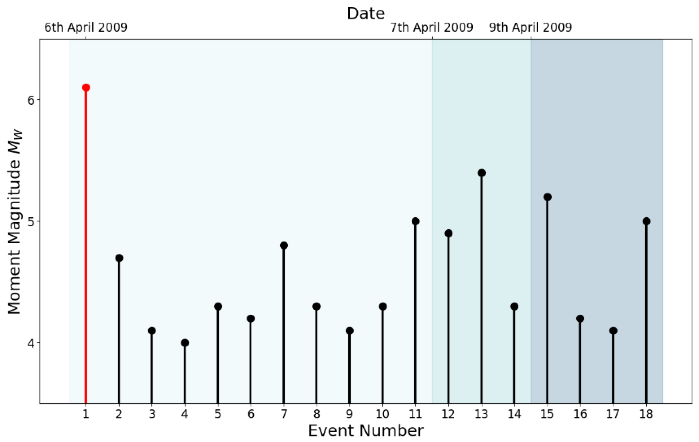
Figure 3.
(a) Map of Italy; (b) An enlargement of the Abruzzo region reporting the epicenters of the 2009 five main shocks, represented as star symbols (the main event is also market with a circle); (c) Geographical position of masonry buildings in the Da.D.O. L’Aquila 2009 dataset [17,18].
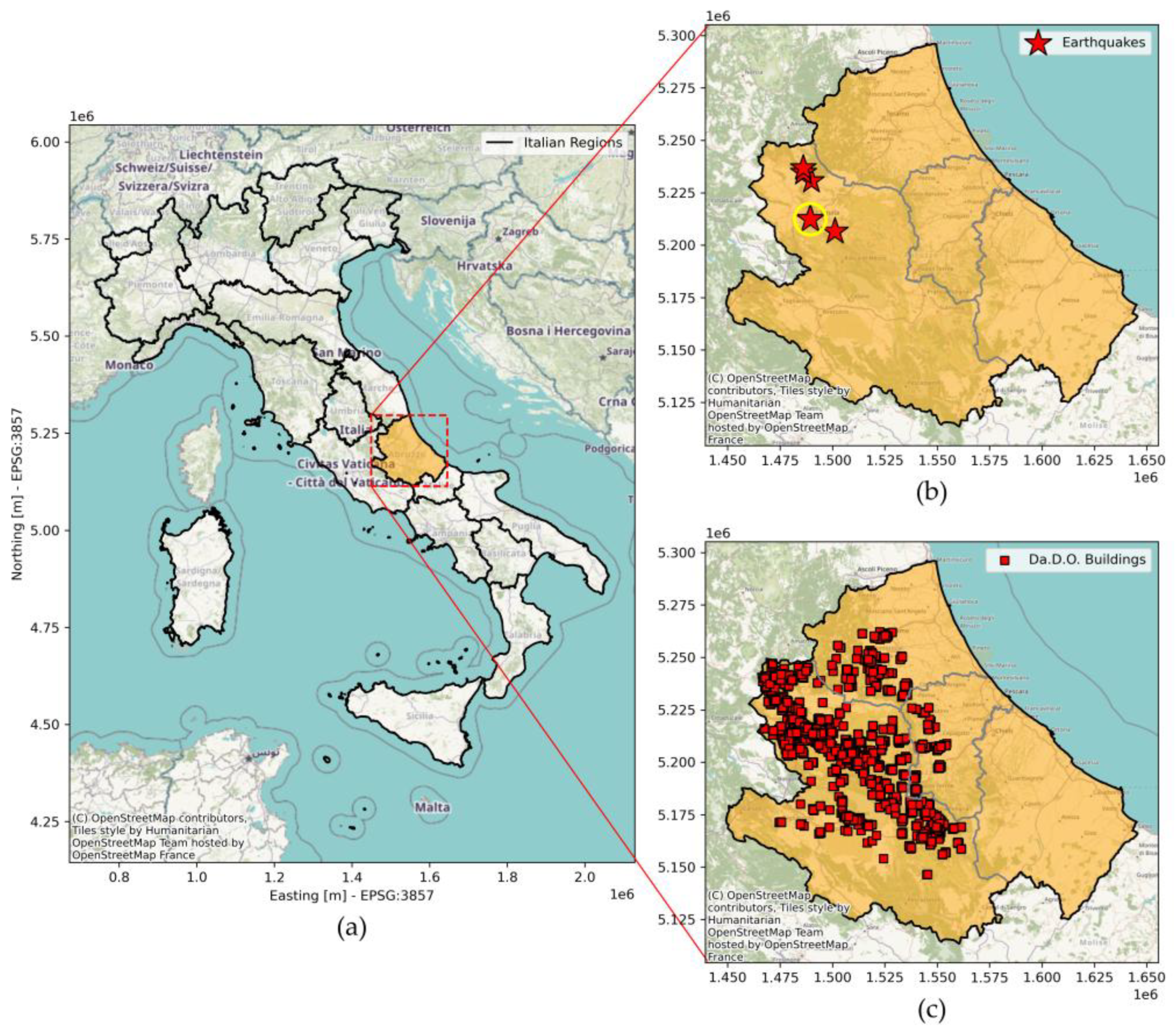
Figure 4.
Percentages of construction types of buildings in the Da.D.O. L’Aquila 2009 dataset [17,18].
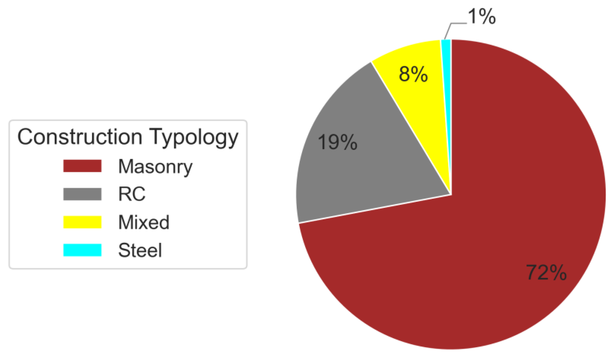
Figure 5.
Overview of key buildings characteristics across construction years. (a) Distribution of buildings by construction year ranges; (b) Percentage distribution of the masonry quality of the vertical structure across construction periods; (c) Percentage distribution of horizontal structure systems across construction years; (d) Percentage distribution of presence of chains across construction years. Data from the Da.D.O. L’Aquila 2009 dataset [17,18].
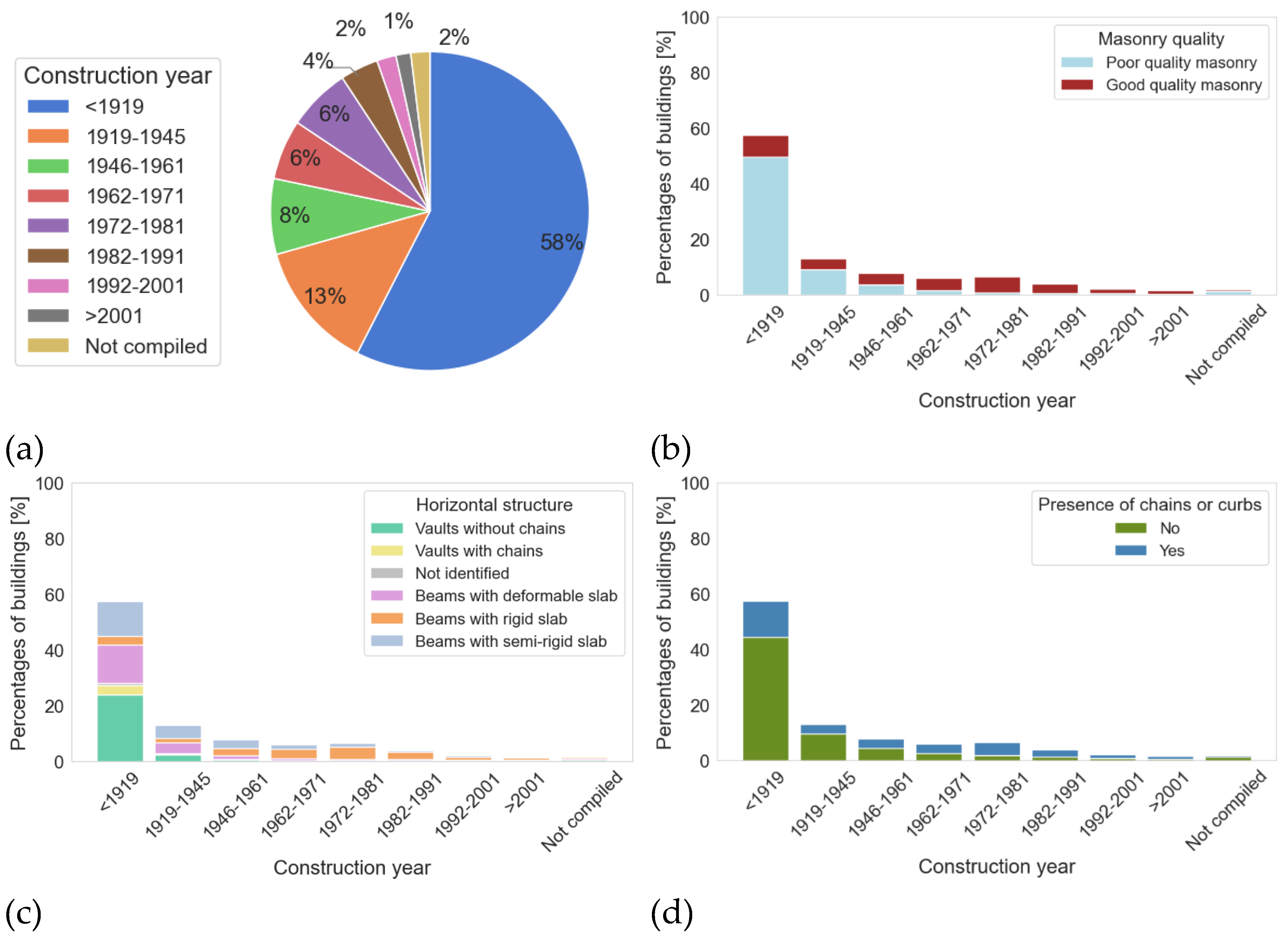
Figure 6.
Different types of horizontal structures: (a) vaulted system, (b) flexible timber slab, (c) rigid slabs with hollow clay blocks concrete.
Figure 6.
Different types of horizontal structures: (a) vaulted system, (b) flexible timber slab, (c) rigid slabs with hollow clay blocks concrete.
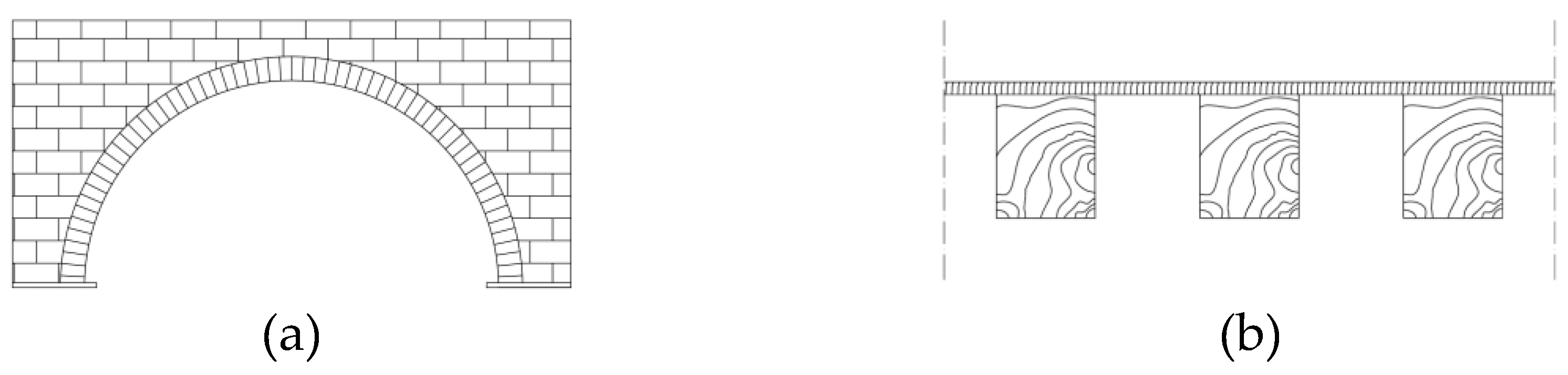
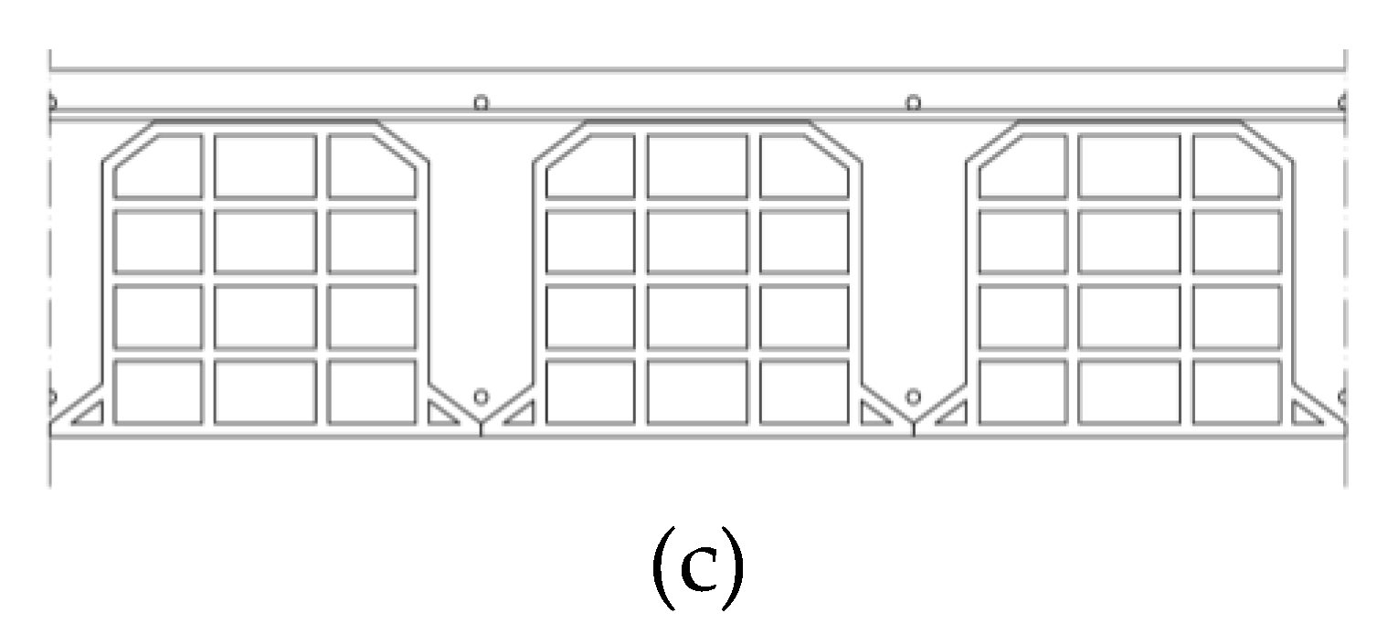
Figure 7.
Distribution of number of floors (a), average floor height (b) and floor area (c). Data from the Da.D.O. L’Aquila 2009 dataset [17,18].
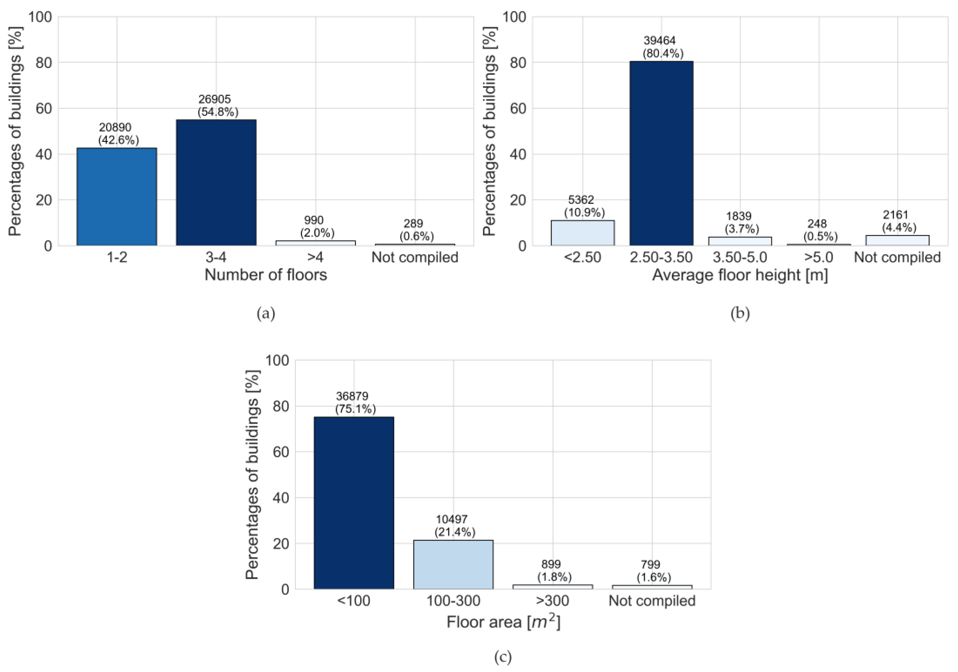
Figure 8.
Distribution of the observed damage levels per vulnerability classes, normal bars represent the damage grade according to the method employed in Da.D.O. (representative of the vertical structures); in hatched bars, the global grade assigned to the buildings using Equation (1).
Figure 8.
Distribution of the observed damage levels per vulnerability classes, normal bars represent the damage grade according to the method employed in Da.D.O. (representative of the vertical structures); in hatched bars, the global grade assigned to the buildings using Equation (1).
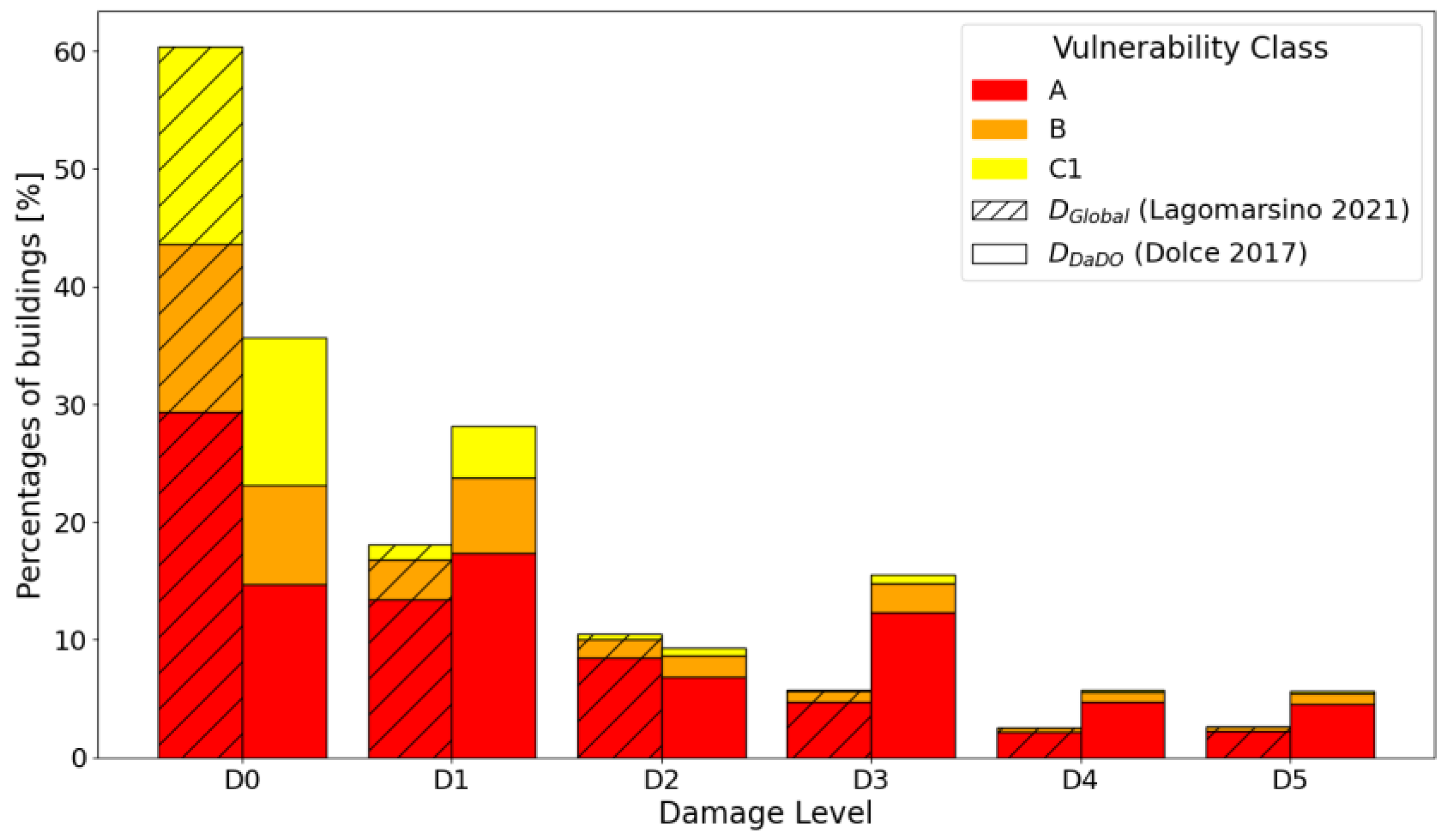
Figure 9.
The vulnerability updated rule proposed in this paper. The initial values are those estimated for the fragility model L21 (Table 3).
Figure 9.
The vulnerability updated rule proposed in this paper. The initial values are those estimated for the fragility model L21 (Table 3).
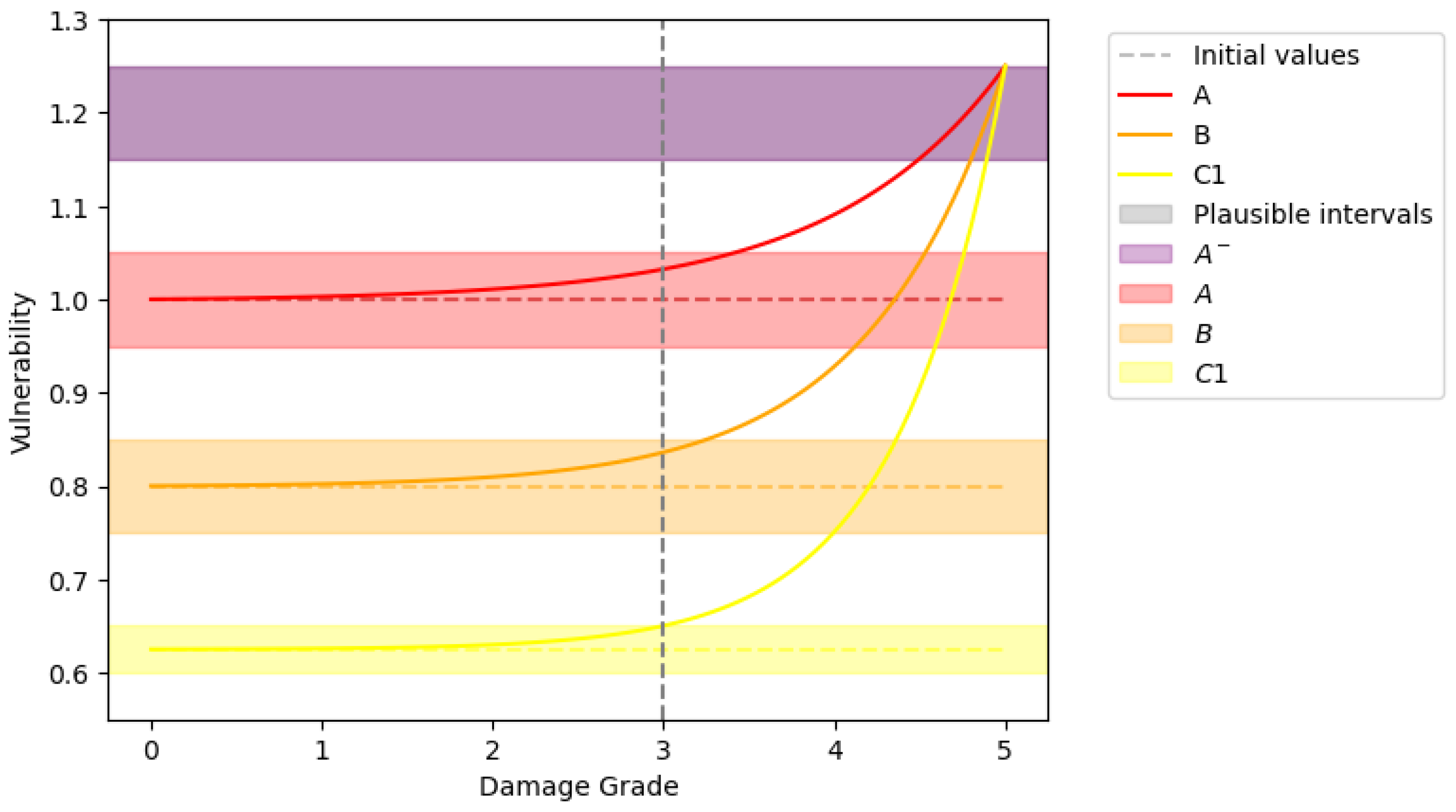
Figure 10.
Distribution of percentage of buildings per vulnerability class and damage level after the mainshock, for P=100%, using the L21 model. See text for details.
Figure 10.
Distribution of percentage of buildings per vulnerability class and damage level after the mainshock, for P=100%, using the L21 model. See text for details.
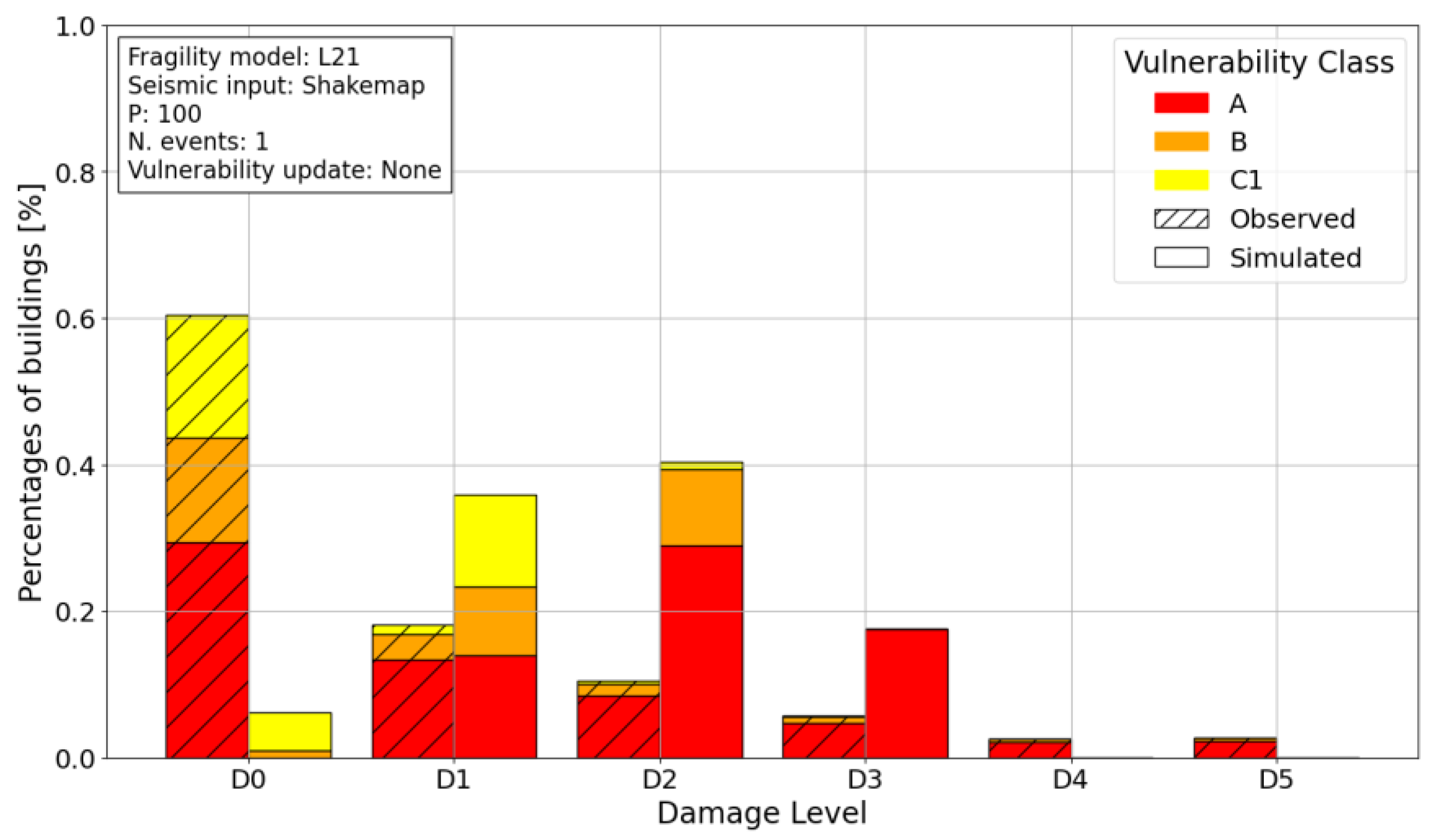
Figure 11.
RMSE values, calculated between the observed and simulated damage distributions for the mainshock scenario, against parameter P from 10% to 100%. The minimum RMSE (3.53) is reached at P=40%.
Figure 11.
RMSE values, calculated between the observed and simulated damage distributions for the mainshock scenario, against parameter P from 10% to 100%. The minimum RMSE (3.53) is reached at P=40%.
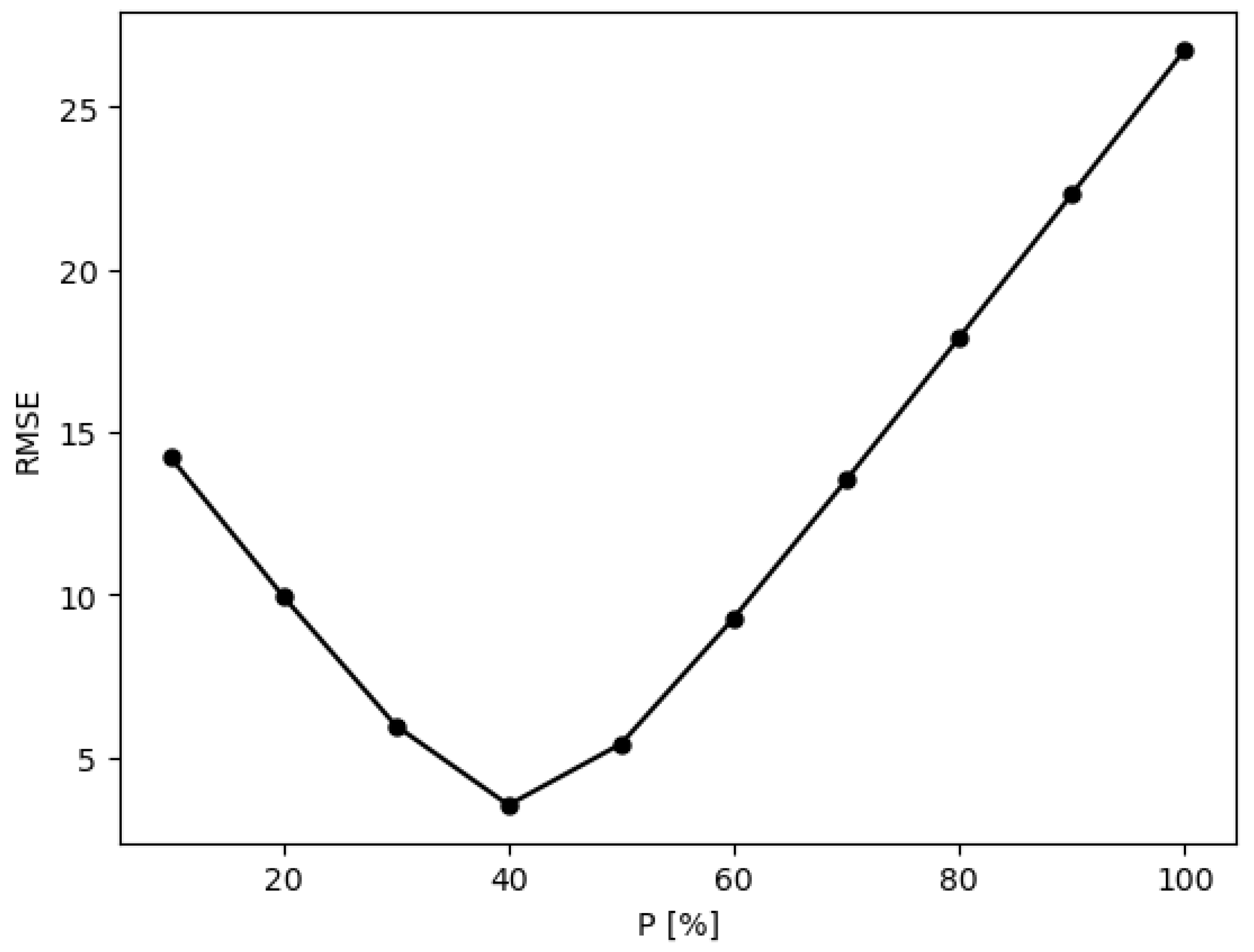
Figure 12.
Comparison between observed and simulated distribution for the mainshock-only scenario with P=40% applying L21. See text for details.
Figure 12.
Comparison between observed and simulated distribution for the mainshock-only scenario with P=40% applying L21. See text for details.
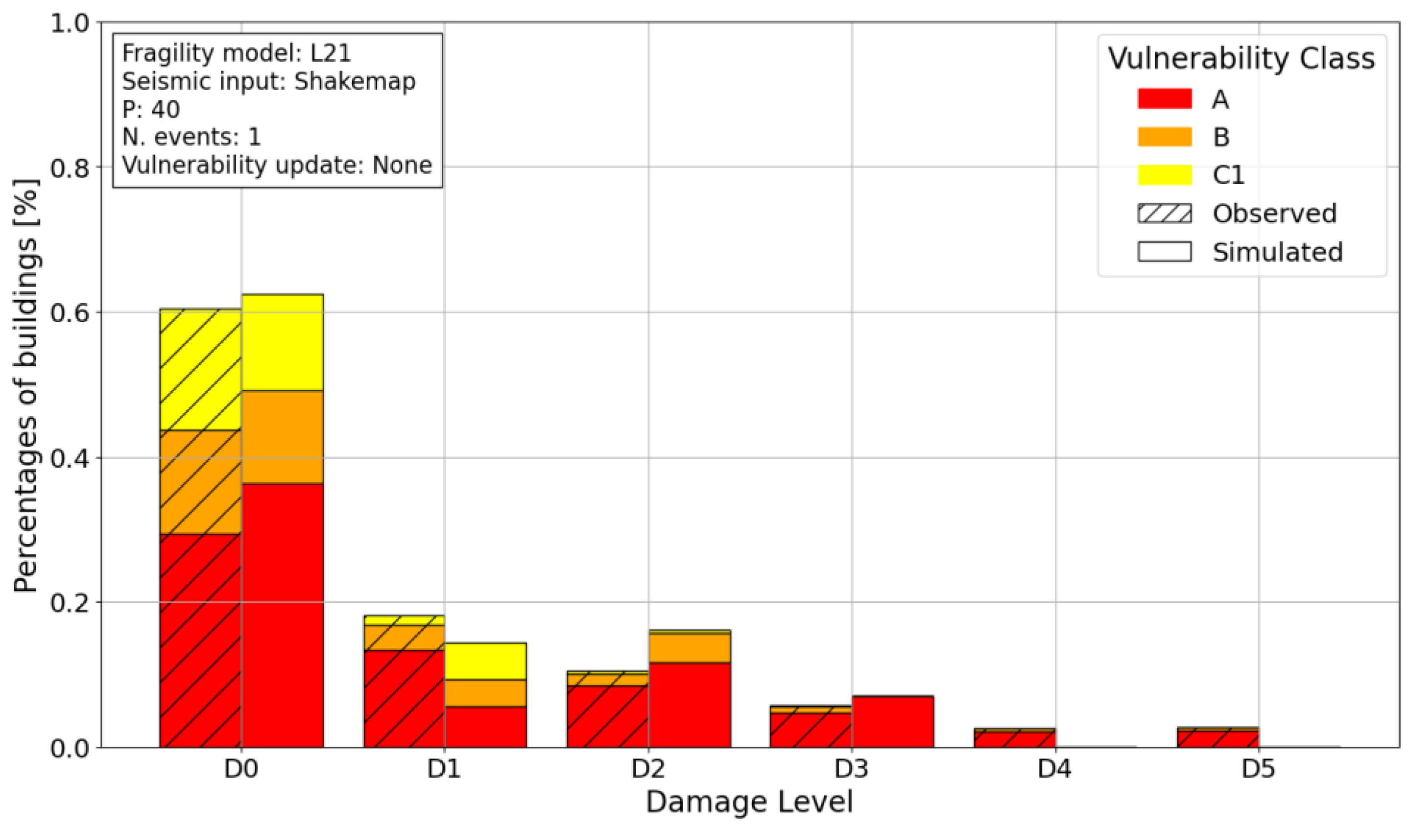
Figure 13.
Stability plot over 100 runs for the mainshock-only scenario using L21 and for P=40%: the mean final damage level (converted from the categorical values D0-D5 to a numerical continuous value in the range 0-5) at the end of each run is averaged with the values of the previous runs.
Figure 13.
Stability plot over 100 runs for the mainshock-only scenario using L21 and for P=40%: the mean final damage level (converted from the categorical values D0-D5 to a numerical continuous value in the range 0-5) at the end of each run is averaged with the values of the previous runs.
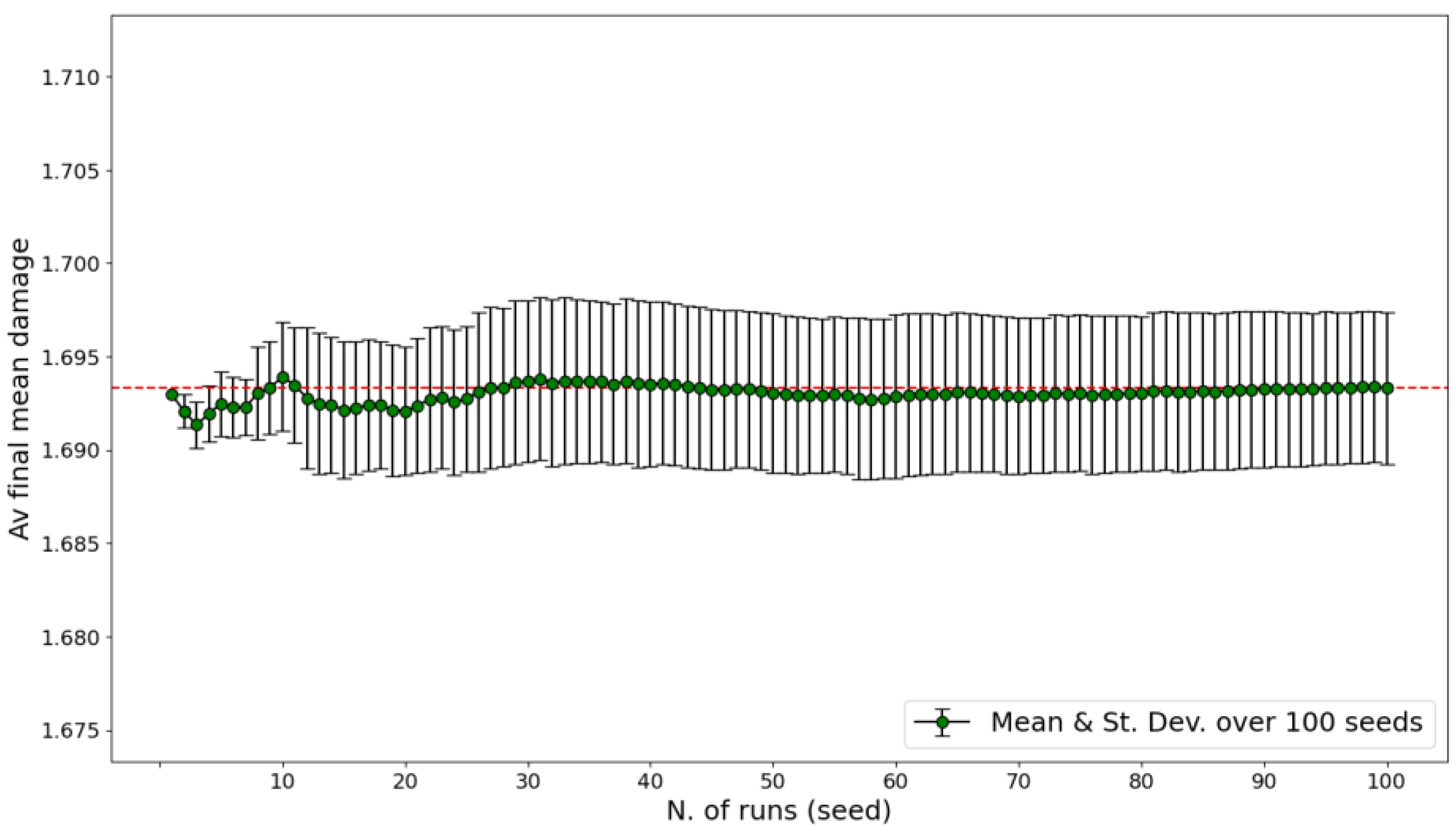
Figure 14.
RMSE values against parameter P from 10% to 100% for fragility model L21 using the vulnerability update rule proposed in this study. The minimum RMSE (2.50) is reached at P=20%. See text for details.
Figure 14.
RMSE values against parameter P from 10% to 100% for fragility model L21 using the vulnerability update rule proposed in this study. The minimum RMSE (2.50) is reached at P=20%. See text for details.
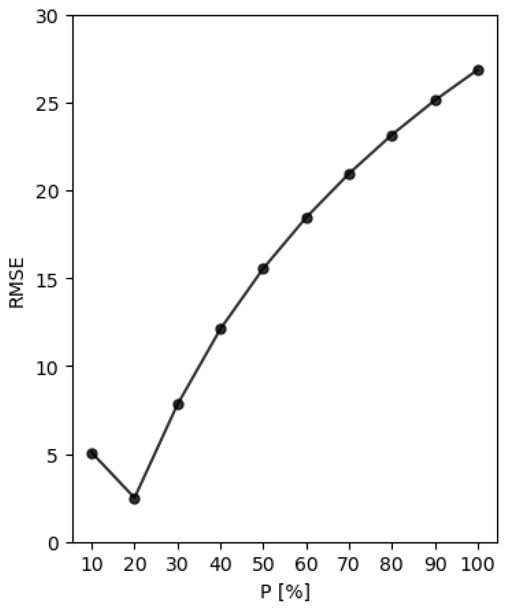
Figure 15.
Distribution of the percentage of buildings per vulnerability class and damage level after the eighteen earthquakes of magnitude greater than Mw 4.0, for P=20%, using the proposed vulnerability update rule.
Figure 15.
Distribution of the percentage of buildings per vulnerability class and damage level after the eighteen earthquakes of magnitude greater than Mw 4.0, for P=20%, using the proposed vulnerability update rule.
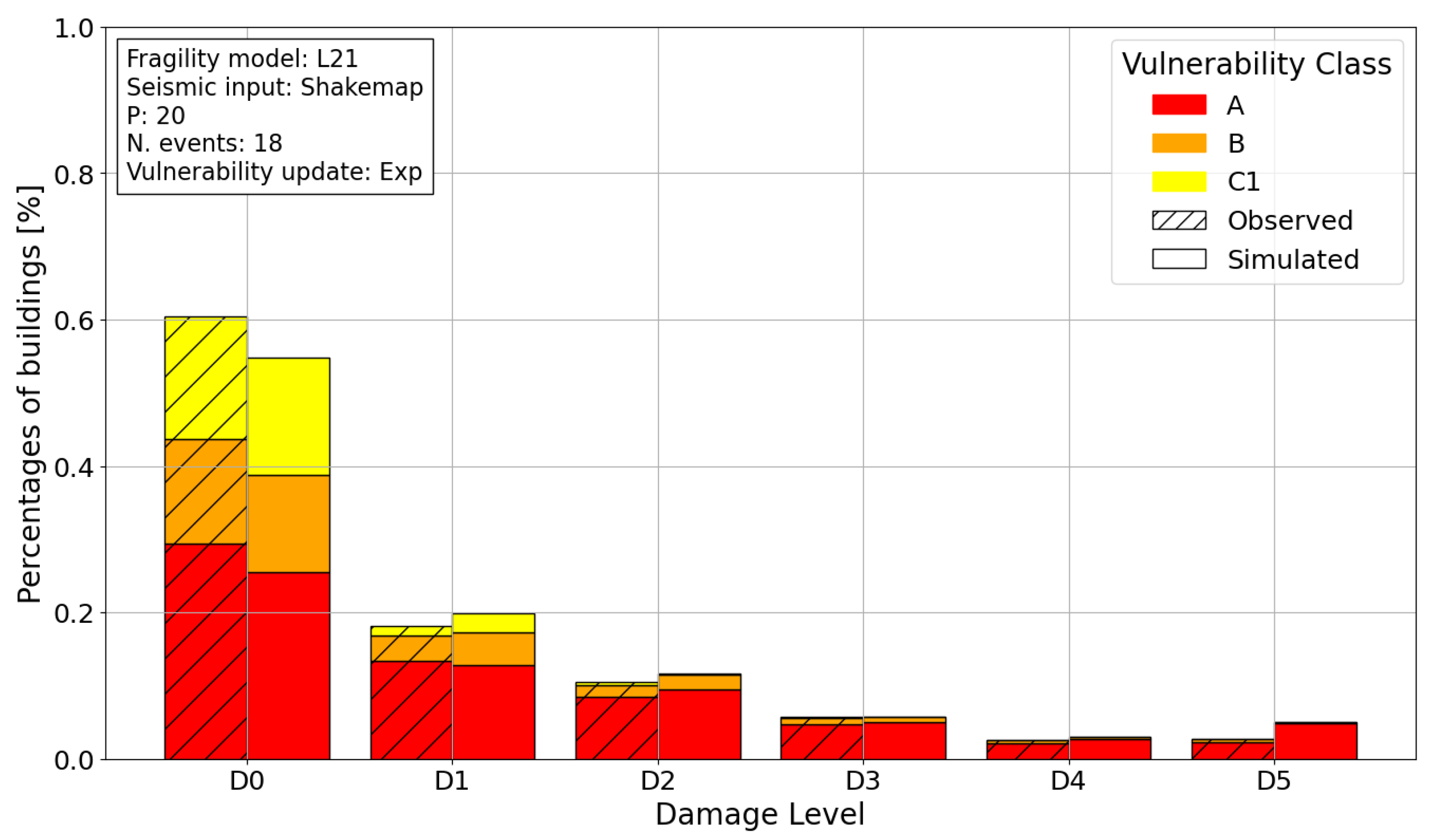
Figure 16.
Stability plot over 100 runs for the 18-event scenario using L21 and for P=20% and exponential vulnerability update rule. See text for details.
Figure 16.
Stability plot over 100 runs for the 18-event scenario using L21 and for P=20% and exponential vulnerability update rule. See text for details.
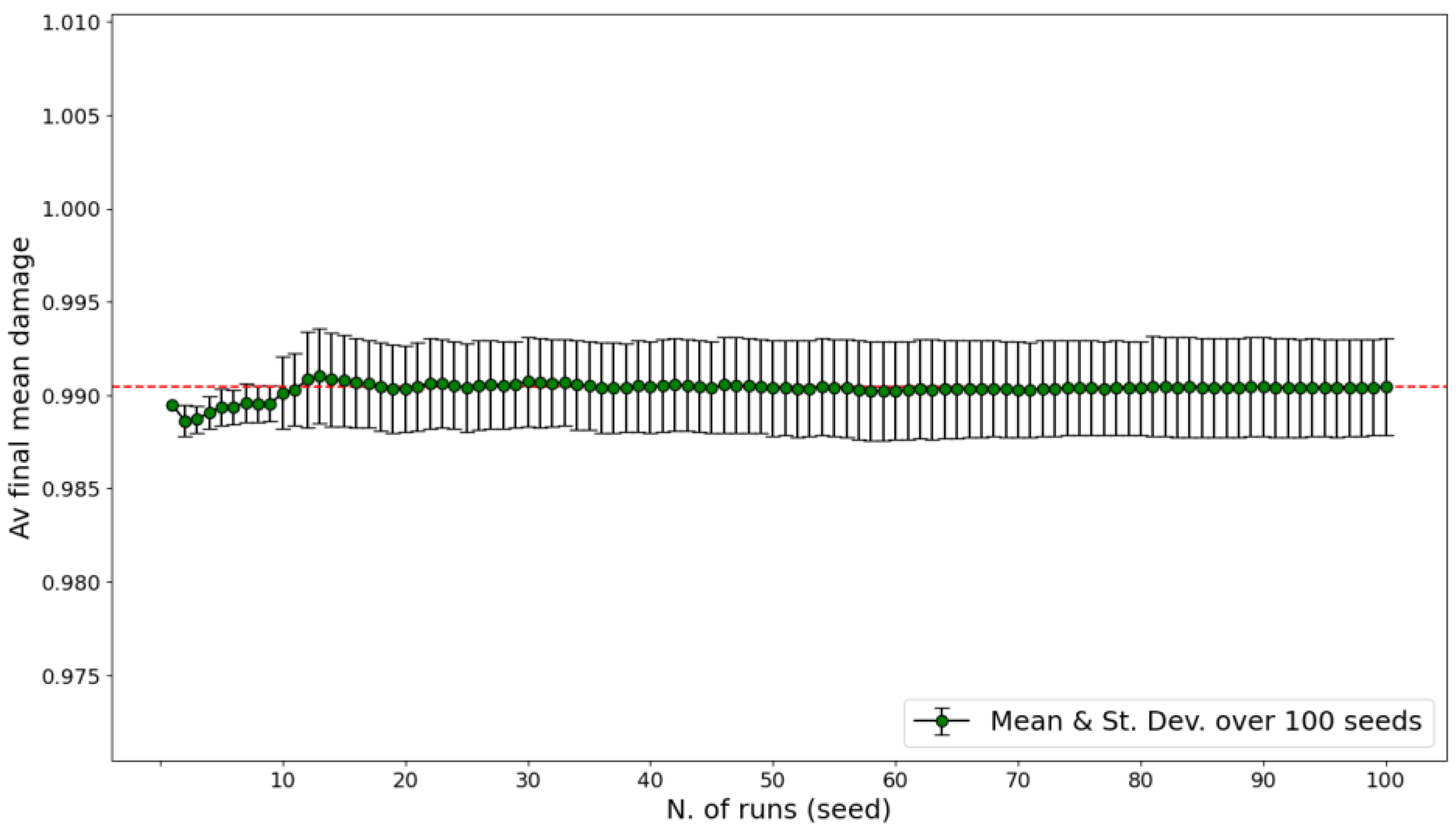

Table 1.
Selected earthquakes from the L’Aquila 2009 sequence.
| Event id | Date [yyyy-mm-dd] |
Time UTC [hh:mm:ss] |
Latitude [°] |
Longitude [°] |
Depth [km] |
Mw | |
| 1 | 1895389 | 2009-04-06 | 01:32:00 | 42.342 | 13.380 | 8.3 | 6.1 |
| 2 | 1895409 | 2009-04-06 | 01:36:39 | 42.352 | 13.346 | 9.7 | 4.7 |
| 3 | 1895419 | 2009-04-06 | 01:40:50 | 42.417 | 13.402 | 11 | 4.1 |
| 4 | 1895429 | 2009-04-06 | 01:41:32 | 42.377 | 13.319 | 8.5 | 4.0 |
| 5 | 1895439 | 2009-04-06 | 01:41:37 | 42.364 | 13.456 | 8.7 | 4.3 |
| 6 | 1895449 | 2009-04-06 | 01:42:49 | 42.300 | 13.429 | 10.5 | 4.2 |
| 7 | 1895879 | 2009-04-06 | 02:37:04 | 42.360 | 13.328 | 8.7 | 4.8 |
| 8 | 1896349 | 2009-04-06 | 03:56:45 | 42.335 | 13.386 | 9.3 | 4.3 |
| 9 | 1897629 | 2009-04-06 | 07:17:10 | 42.356 | 13.383 | 9 | 4.1 |
| 10 | 1901099 | 2009-04-06 | 16:38:09 | 42.363 | 13.339 | 10 | 4.3 |
| 11 | 1903809 | 2009-04-06 | 23:15:00 | 42.463 | 13.385 | 9.7 | 5.0 |
| 12 | 1906339 | 2009-04-07 | 09:26:28 | 42.336 | 13.387 | 9.6 | 4.9 |
| 13 | 1908319 | 2009-04-07 | 17:47:00 | 42.303 | 13.486 | 17.1 | 5.4 |
| 14 | 1909629 | 2009-04-07 | 21:34:29 | 42.364 | 13.365 | 9.6 | 4.3 |
| 15 | 1916789 | 2009-04-09 | 00:52:00 | 42.489 | 13.351 | 11 | 5.2 |
| 16 | 1917479 | 2009-04-09 | 03:14:52 | 42.335 | 13.444 | 17.1 | 4.2 |
| 17 | 1917839 | 2009-04-09 | 04:32:45 | 42.445 | 13.434 | 9.8 | 4.1 |
| 18 | 1921649 | 2009-04-09 | 19:38:00 | 42.504 | 13.35 | 9.3 | 5.0 |
1 Data from the INGV ShakeMap Archive.
Table 2.
Vulnerability classes of masonry buildings evaluated on the basis of some of their structural features, following the indications present on the Da.D.O. web platform [17,18]. Adapted from Table 4.8 of the 2022 Da.D.O. User Manual.
| Vulnerability Class | Vertical structure | Horizontal structure | Chains |
| A | Bad quality | Vaults without chains, vaults with chains, deformable slab, semi-rigid slab, unidentified | No |
| Bad quality | Vaults without chains, unidentified | Yes | |
| Good quality | Vaults without chains, vaults with chains, deformable slab, unidentified | No | |
| B | Bad quality | Rigid slab | No |
| Bad quality | Vaults with chains, deformable slab, semi-rigid slab, rigid slab | Yes | |
| Good quality | Semi-rigid slab | No | |
| Good quality | Vaults without chains, vaults with chains, deformable slab, unidentified | Yes | |
| C1 | Good quality | Rigid slab | No |
| Good quality | Semi-rigid slab, rigid slab | Yes |
Table 3.
Vulnerability indices. Adapted from Table 10 in [35] and modified for vulnerability class C1.
Table 3.
Vulnerability indices. Adapted from Table 10 in [35] and modified for vulnerability class C1.
| Vulnerability Class | Plausible range |
| A | 0.95–1.05 |
| B | 0.75–0.85 |
| C1 | 0.60–0.65 |
Table 4.
Proposal of plausible range of initial vulnerability for the L21 fragility model.
| Vulnerability Class | plausible range |
| A- | 1.15–1.25 |
Disclaimer/Publisher’s Note: The statements, opinions and data contained in all publications are solely those of the individual author(s) and contributor(s) and not of MDPI and/or the editor(s). MDPI and/or the editor(s) disclaim responsibility for any injury to people or property resulting from any ideas, methods, instructions or products referred to in the content. |
© 2025 by the authors. Licensee MDPI, Basel, Switzerland. This article is an open access article distributed under the terms and conditions of the Creative Commons Attribution (CC BY) license (http://creativecommons.org/licenses/by/4.0/).
Copyright: This open access article is published under a Creative Commons CC BY 4.0 license, which permit the free download, distribution, and reuse, provided that the author and preprint are cited in any reuse.


