Submitted:
01 October 2025
Posted:
01 October 2025
You are already at the latest version
Abstract
Accurate determination of the target strength (TS) of a fish species is essential for estimating the biomass of fish stocks using acoustic technology. This study estimated the daytime in situ target strength of Pacific hake (Merluccius productus) at 38 kHz using echosounder data collected during hake biomass acoustic trawl surveys and research cruises conducted from 2009 to 2019 by U.S. and Canadian scientists. The intercept term for the 20-log TS regression over fish length at 38 kHz, b_20, was found to be -67.9 dB re 1 m2 (CI: -68.09, -67.72) closely aligning with the currently used value of -68 dB in biomass assessments. Applying the revised b_20 value of -67.9 dB in past stock assessments suggests that biomass estimates would be underestimated by less than 3%, which is well within the typical uncertainty range of fish stock assessments.
Keywords:
hake
; echosounder
; in situ target strength
; biomass estimate
1. Introduction
Effective management of fisheries and ecosystems requires marine scientists to take on substantial responsibilities, including monitoring, assessing, and researching marine resource distributions. Pacific hake (Merluccius productus), hereafter referred to as hake, is a commercially important marine fish found off the west coast of North America (Longo et al., 2024). Over the past decade (2014-23), coastwide annual harvests averaged 338,606 metric tons (Grandin et al., 2024), with U.S. and Canadian catches averaging 275,957 metric tons and 62,648 metric tons, respectively. In 2023, the coastwide catch reached 263,981 metric tons (Grandin et al., 2024). The U.S. West Coast's hake fishery, including non-tribal at-sea and shoreside operations, supported 4,450 jobs and generated an income of $335 million in 2021.
Beyond its commercial significance, hake is a key trophic species and the most abundant groundfish in the California Current Large Marine Ecosystem (Sherman, 1991). Given its prominent economic and ecological value, integrated acoustic trawl (IAT) surveys have been conducted to assess hake's abundance, spatial and temporal distributions, and additional biological characteristics along the west coasts of the United States and Canada (Fleischer et al., 2005). These surveys began in 1977, with the Alaska Fisheries Science Center (AFSC) conducting triennial IAT surveys in U.S. and Canadian waters. In 1990, Fisheries and Oceans Canada (DFO) initiated annual IAT surveys in Canadian waters. After the 2001 survey, responsibility for the U.S. portion of the IAT survey transitioned to the Northwest Fisheries Science Center (NWFSC), and the survey frequency increased from triennial to biennial. Since 1995, the United States and Canada have collaborated on hake assessments. The triennial IAT surveys of 1995, 1998, and 2001 were conducted jointly by AFSC and DFO, while surveys since 2003 have been conducted by NWFSC and DFO. The joint hake surveys normally began at Point Conception, California (the current southern extent of the survey area) and proceeded north along the west coast of the U.S. and Canada, surveying Queen Charlotte Sound, Hecate Strait (above Port Hardy in Fig.1), Dixon Entrance (the northern extent of the survey area, straddling the Canada and Alaska border), and the west side of Haida Gwaii, which was surveyed from north to south (Figure 1, with the actual 2019 survey transects).
Estimating the abundance or biomass of fish stocks using acoustic technology requires accurate measurements of an acoustic property known as target strength (TS). TS is directly tied to biomass estimates, which are based on echo integration theory (Scherbino and Truskanov, 1966). Conceptually, TS measures the acoustic energy scattered (typically in the backward direction) from an object relative to the source intensity (Medwin and Clay, 1998).
Three common methods are used to estimate the TS of fish: in situ field data (Ona, 1995; Gauthier and Rose, 2002; Peña, 2008; Kloser et al., 2011; Madirolas et al., 2017), ex situ data (Kang and Hwang, 2003; Henderson and Horne, 2007; Boswell and Wilson, 2008;), and theoretical model predictions (Love, 1978; Foote, 1985; Clay and Horne, 1994; Jech et al., 2015; Chu, 2024). The target strength currently used by NWFSC and DFO to estimate hake biomass was originally published by Traynor (1996). This value was derived from in situ hake echosounder data at 38 kHz using a widely accepted 20-log regression formula based on the theoretical relationship between the differential backscattering cross section () and fish length () . In the case of Pacific hake, L represents fork length. The TS is commonly expressed logarithmically as:
where fish length is measured in centimeters, and the intercept term is in dB re 1m2. The b20 that has been used by NWFSC/DFO for Pacific hake biomass estimates has been historically set to -68 dB based on in situ target strength values reported by Traynor (1996). However, this intercept value was questioned by Henderson and Horne (2007), where a much smaller was suggested.
To address discrepancies in estimates and evaluate the validity of the currently used b20, we analyzed in situ echosounder TS data from single targets collected between 2009 and 2019 during hake biomass surveys and research cruises. In contrast to Henderson and Horne (2007), which used a combination of ex situ and nighttime in situ methods (similar to Traynor (1996)) to estimate target strength, this study focused on daytime in situ methods as being more representative of fish encountered during the daytime survey used for stock assessment, and also provided estimates of accuracy and robustness. To account for bias due to multiple target scattering and low signal to noise ratio (SNR) typically encountered during daytime surveys (when fish are found in denser aggregations at greater depth) we have used a stepwise approach for selecting valid targets and further introduced a pulse energy filtering method.
2. Materials and Methods
2.1. Data Description
Acoustic data were collected between 2009 and 2019 using EK60 split-beam echosounders manufactured by Kongsberg Simrad. This study focused on data collected at 38 kHz, the primary frequency used for hake biomass estimation and widely recognized for fish biomass assessments globally. Single-fish TS measurements were collected during midwater trawl verifications tows conducted at an average vessel speed of approximately 3 knots (~1.5 m/s) using the NOAA Fisheries Survey Vessel (FSV) Bell M. Shimada. Only trawls in which hake exceeded 95% of the total catch composition (by weight) were selected for TS analysis.
In addition, a Dropped Acoustic Information SYstem (DAISY), a deployable instrument, was used to collect echosounder data off the Canadian Coast Guard Ship (CCGS) W. E. Ricker (Inset in Fig. 1). DAISY consisted of 38-kHz and 120-kHz split-beam EK60 echosounders connected to a power supply inside a pressure housing. The unit was equipped with 200 m of cable for deployment at depth using a relay for topside control and included a heading, pitch, and roll sensor. The CCGS W. E. Ricker drifted while the DAISY was deployed to collect data. Each deployment of DAISY was associated with midwater verification trawl. Catches of hake from these trawls comprised 80%, 82%, and 99% of the total catch for September 7, 2014, September 14, 2014, and March 23, 2016, respectively. An in-trawl camera system indicated that the other species caught in 2014 (mostly opalescent inshore squid, Dorytheutis opalescens) were in different depth layers than the hake. The geographic locations of all selected trawls used for hake in situ target strength estimation are shown in Fig. 1. Echosounders from the Shimada and DAISY transmitted narrowband pulses with a duration of 1.024 ms. All echosounders were calibrated using the standard sphere method (Demer et al. 2015) prior to each survey, including the deployment of calibration sphere at depth for DAISY measurements.
2.2. Data Analysis
To correctly obtain single target TS data, the Single Target detection algorithm of Echoview (version 13.1) was used (Table 1). The single targets that fell within these parameters only served as foundation for further analysis. Originally, we used the fish tracking algorithm provided within Echoview (Table 2), based on the Alpha-Beta tracking algorithm described by Blackman (1986), but inspections revealed a high number of erroneous tracks which required substantial manual corrections, despite several attempts at fine-tuning the tracking parameters. To better ensure the TS samples in the selected fish tracks were from individual fish, we manually selected candidates from these fish tracks, following stringent guidelines to guarantee the quality of the samples for final TS analysis. The guidelines for single targets based on initial fish tracks analysis were:
1. Fish tracks were selected throughout the depth range of aggregations but primarily from the outskirts of fish aggregations away from regions of highest densities (generally the center of aggregations) to minimize potential biases from multiple-targets.
2. Each fish track had to contain at least five contiguous echoes.
3. Following track selection, only targets that were within 2° of the acoustic beam axis were retained for further analyses.
4. Sample TS values greater than -30 dB were excluded to eliminate larger, non-hake targets or potential multiple targets.

Table 1.
EK60 echosounder parameters for Single Target Detection.
| Single Target Detection | |
|---|---|
| General parameters | Parameter Value |
| TS Threshold (dB) | -60 |
| Pulse length determination level (dB) | 6.0 |
| Minimum normalized pulse length | 0.2 |
| Maximum normalized pulse length | 1.8 |
| Beam compensation | |
| Beam compensation model | Simrad LOBE |
| Maximum beam compensation (dB) | 12.0 |
| Exclusion | |
| Maximum standard deviation of | |
| Minor-axis angles (deg) | 2.0 |
| Major-axis angles (deg) | 2.0 |
Table 2.
EK60 initial target tracking parameters.
| Direction on a 3-d orthogonal frame | Major axis | Minor axis | Depth |
|---|---|---|---|
| α | 0.7 | 0.7 | 0.7 |
| β | 0.5 | 0.5 | 0.5 |
| Exclusion distance (m) | 4.0 | 4.0 | 0.4 |
| Weights | 30 | 30 | 40 |
| Minimum number of single targets | 3 | ||
| Minimum number of pings | 3 | ||
| Maximum gap (pings) | 1 | ||
Following the selection of the TS samples satisfying these criteria, additional filtering was applied using a pulse-energy detection range on each single target. The reasoning of using this pulse-energy criterion was based on the concept that if the echoes from two targets (or multiple targets) were either in or out of phase but arrived at slightly different time, the resultant echo would be either elongated or shortened, respectively, but still within the Single Target Detection pulse duration window specified in Table 1. As a result, the combined and normalized pulse-energy over a time window of the transmit pulse duration would likely be either greater or less than the normalized transmit pulse-energy over the duration of the transmit pulse (1.024 ms in this study). The pulse energy () was calculated as:
where is the echo intensity, which is proportional to the volume backscattering coefficient, , where is the volume backscattering strength. Since the absolute value of depends on the target, we used a normalized and the normalized pulse energy in the actual algorithm:
where is the number of samples in each transmitted pulse (4 in the case of Simrad EK60 system) and is the normalized of the pulse of interest. TS samples were retained if their pulse energy satisfied the relation:
where and are the theoretical mean and the standard deviation of the normalized echo energy, respectively, and were estimated based on the recorded waveform of the EK60 transmit pulse presented in Figure 2.30 in Demer et al. (2017). Since each pulse in the EK60 has four samples, the start of a (theoretical) echo was randomized within the first 256 μs time window of the pulse (equivalent to 1/4 of a 1024 μs pulse length). 10,000 realizations of this randomized start time were used in estimating the theoretical and with values of 3.56 and 0.14, respectively.
Biological catch data were matched with acoustic data by assigning the mean fork length from each trawl to corresponding single-fish TS samples. Only trawls in which the fork length distribution of hake was relatively unimodal and had a standard deviation of less than 5 cm were retained for analyses.
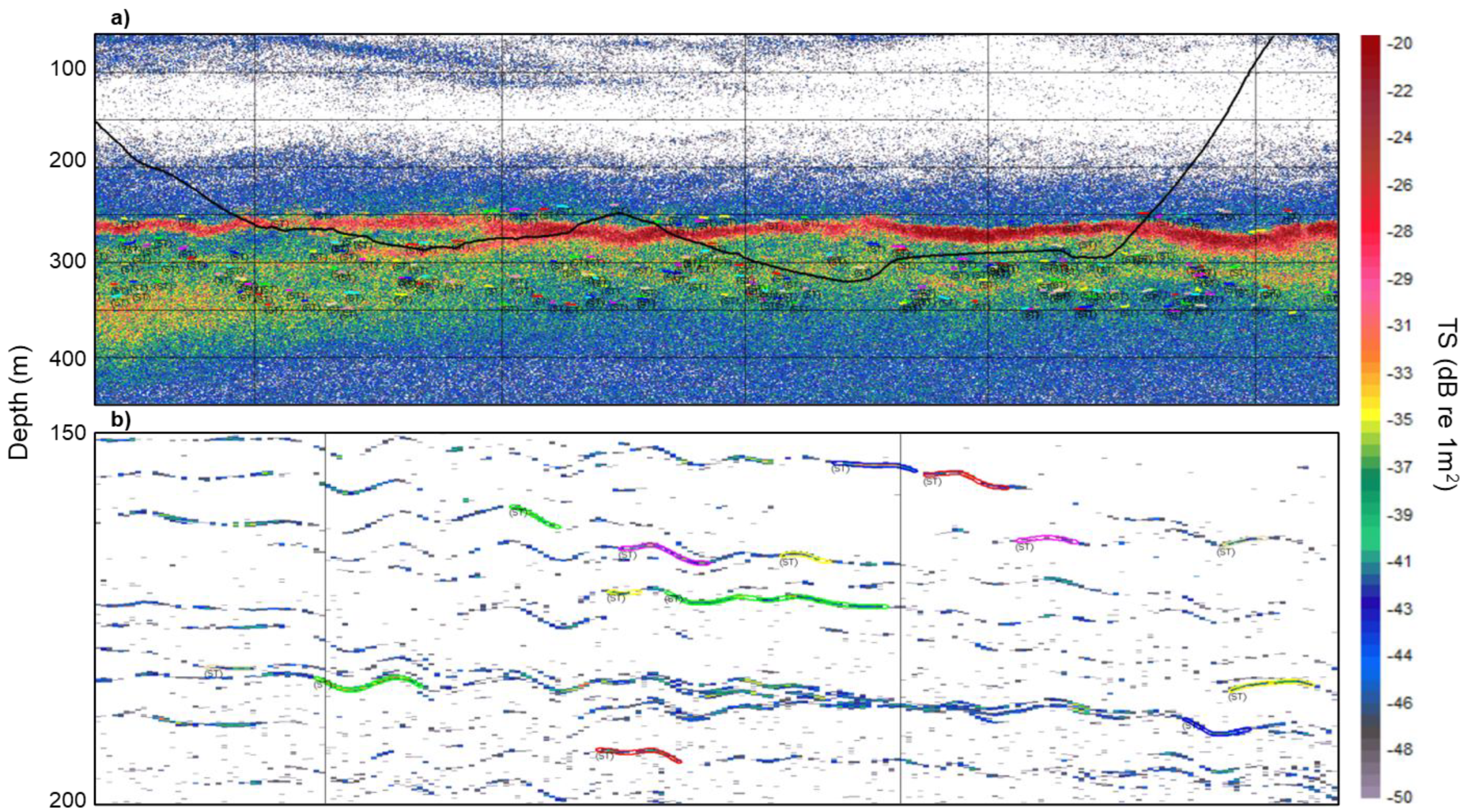
Representative echograms illustrating single-target detections are shown in Figure 2, where the trawl traces were superimposed onto the echogram (Figure 2a) and the chosen TS samples from single fish were away from the center of the fish aggregation, the region with the highest fish density. The single-fish TS were much easier to determine from the echograms collected with DAISY due to the slow vessel speed (Figure 2b). As a result, the detected single-fish TS echo-traces were much longer than those collected when trawling at a ship speed of about 3 kts (~ 1.5 m/s).
Figure 2.
Examples of the Target Strength echograms from assumed individual hake, where each colored line (polygons) indicates an individual track. (a) Collected from the U.S. Fisheries Survey Vessel (FSV) Bell M. Shimada during a trawl (trawl path is indicated by the thick black line). Each vertical bar indicates 0.5 nmi; (b) DAISY drift TS echogram deployed from the CCGS W. E. Ricker, each vertical line representing 100 pings. Depth (in m) is indicated on the left side.
2.3. Estimation of
To obtain an optimized estimate of the intercept, , we used the least-square fit to the TS data using Eq. (1), a 20-log form of the TS-length regression relation. The mean fork length (from trawl samples) was categorized in 1 cm length bins. Since the only unknown is the intercept term , it is straightforward to show that using the standard least-square approach, can be estimated by
where is the total number of length bins and is the number of length samples in each length bin (which may have included more than one trawl when their mean length was within the same 1 cm bin). and are the measured TS (dB) value and the corresponding hake fork length (cm) for the ith length bin and jth TS sample in the ith length bin, respectively. For comparison, the TS-length regression was also assessed empirically with a free slope parameter in the form of:
Where a is the slope parameter and ba its associated intercept.
2.4. Statistical Analysis
To evaluate the variability and robustness of the estimate, three statistical methods were applied and compared. Each methods provide a slightly different perspective on the sampled data and their reliability:
1. Resampling: all TS data were randomly resampled with non-replacement, using 95%, 90%, and down to 5% of the original data, with 1,000 realizations for each percentage bracket. This addresses the sensitivity of the data to marginally high or low TS samples (or specific to trawl hauls) by assessing significant divergence in slope estimates as the TS sample size is gradually reduced down to a small fraction of all available data. This resampling approach also helps in identifying potential bias due to outliers, or disproportionate weight to sample values that are at the tail end of the distribution (e.g., hauls with the smallest and largest mean fork lengths).
2. Bootstrapping: The bootstrap method estimated the sampling distribution of by resampling the original data using all (100%) data samples with replacement (Horowitz, 2019; Efron and Tibshirani, 1993), also with 1,000 realizations.
3. Jackknife: The jackknife cross-validation technique, a leave-one-out resampling method with replacement, was used for bias and variance estimation (Jones, 1974).
3. Results and Discussion
3.1. Target Strength (TS) Data Processing and Acceptance
After applying the Single Target Detection and tracking criteria specified in Table 1 and Table 2, the manual selection guidelines, and a pulse-energy filter, the processed TS samples were analyzed. The accepted TS samples from assumed single targets associated with the selected hauls across different years are summarized in Table 3. The dataset comprises a total of 92 hauls from 13 surveys conducted between 2009 and 2019, with an overall acceptance rate of single targets less than 2%. This was largely due to the pulse energy filter, which we found necessary to analyze target at long range in low signal to noise ratio conditions, because of the relatively high density of hake (and other scatterers) at depth during daytime surveys. The average biological catch per haul was approximately 380 kg, with an average hake catch composition of 98%, confirming that the samples were representative of hake-dominated areas. Exceptions were two hauls in 2014 that were associated with the DAISY data, where hake catch proportions were slightly above 80% (Table A1). Although the hake catches were lower for these DAISY data, the non-hake catches were primarily squids (no gas inclusions) and small lanternfish (~ 5-cm), whose TS were believed to be much less than those of hake (). Furthermore, in-trawl camera footage indicated that these non-hake animals were caught at different depths from hake, as explained in Sec. 2.1.
3.2. TS Distribution and Depth Analysis
The histogram of the TS samples from detected single targets is shown in Figure 3. The TS distribution was not symmetric around the mean or mode, approximately at -37.5 dB. A small portion of the TS samples had very low TS values, indicating the TS samples were either from smaller hake individuals, from hake that had larger tilt angles, or from small non-hake targets. Although the lower limit of the Single Target Detection algorithm was specified at -60 dB re 1 m2, the actual accepted TS samples following the filtering processes were all greater than -55 dB re 1 m2.
TS samples distributed between 150 and 400 m represented about 80% of the total accepted TS values (Figure 4). There were few samples detected in very shallow water, i.e., shallower than 100 m depth, but their corresponding TS values were mostly lower than -45 dB re 1 m2, significantly lower than the mean TS value of -36.8 dB re 1 m2, or the median value of -36.3 dB re 1 m2 (Figure 5), likely from smaller age-1 juvenile hake, or even age-0 young-of-year (YOY) hake.
3.3. Spatial Variability and Fork Length Association
Except for TS samples around lat 43.5°N, where the TS values were lower and more spread out, all TS samples had median values close to the overall median of -36.9 dB re 1 m2 (Figure 6). These low TS values at lat 43.5°N possibly correspond to the smaller hake fork length at the same latitude (Figure 7) as stated in Section 3.2. Some trawls at the median length were at the higher end of the 75th percentile (lat 36.5°N, 38.5°N, 39°N, 41°N, and 43.5°N), or at the lower end of the 25th percentile (lat 37.5°N, 42°N, 42.5°N, and 44°N). At some latitudes, the 25th and 75th percentiles and the median were identical (lat 41.5°N and 45.5°N), indicating that the catches were uniform in length distribution.
3.4. TS-Length Regression
One of the most important results of this study is the regression of TS versus length. The regression was performed in the logarithmic domain for TS (dB) and linear domain for the length (cm) (Section 2.3). The boxplot of the TS values of the accepted samples as a function of length is presented in Figure 8. Mean length from trawls were categorized in 1 cm length bins, which may include samples from more than one trawl (when their mean length was similar). The 20-log regression formula with a b20 of -67.9 dB is only 0.1 dB larger than the value derived from Traynor et al. (1996) currently used for biomass estimates of Pacific hake. Since the areal acoustic scattering coefficient (NASC) is used for converting the acoustic quantity to biological quantity, i.e., the number of fish:
where is the differential scattering cross section defined in Eq. (1), or . For a fixed NASC value, difference in will result in a change in number of fish, N:
A relative change in estimated fish number is the ratio of (8) to (7):
As a result, a 0.1 dB increase in TS would lead to less than 3% in estimated fish number. Applying this revised value and assuming that the fish weight is proportional to fish number, the estimated biomass would have been less than 3% higher than the acoustic biomass estimates reported from previous Joint U.S.-Canada IAT Surveys (Grandin et al., 2024).
Figure 8.
Target strength (TS) from single targets as a function of length. The x-axis is marked and labelled at the mean fork length of the samples. The fitted TS-length regression (solid magenta line) is superimposed onto the plot, and the upper and lower 95% Confidence Intervals of the samples values in each length category are plotted with a dashed line (dashed green line). A non-20-log regression (dashed black) is also superimposed to the plot.
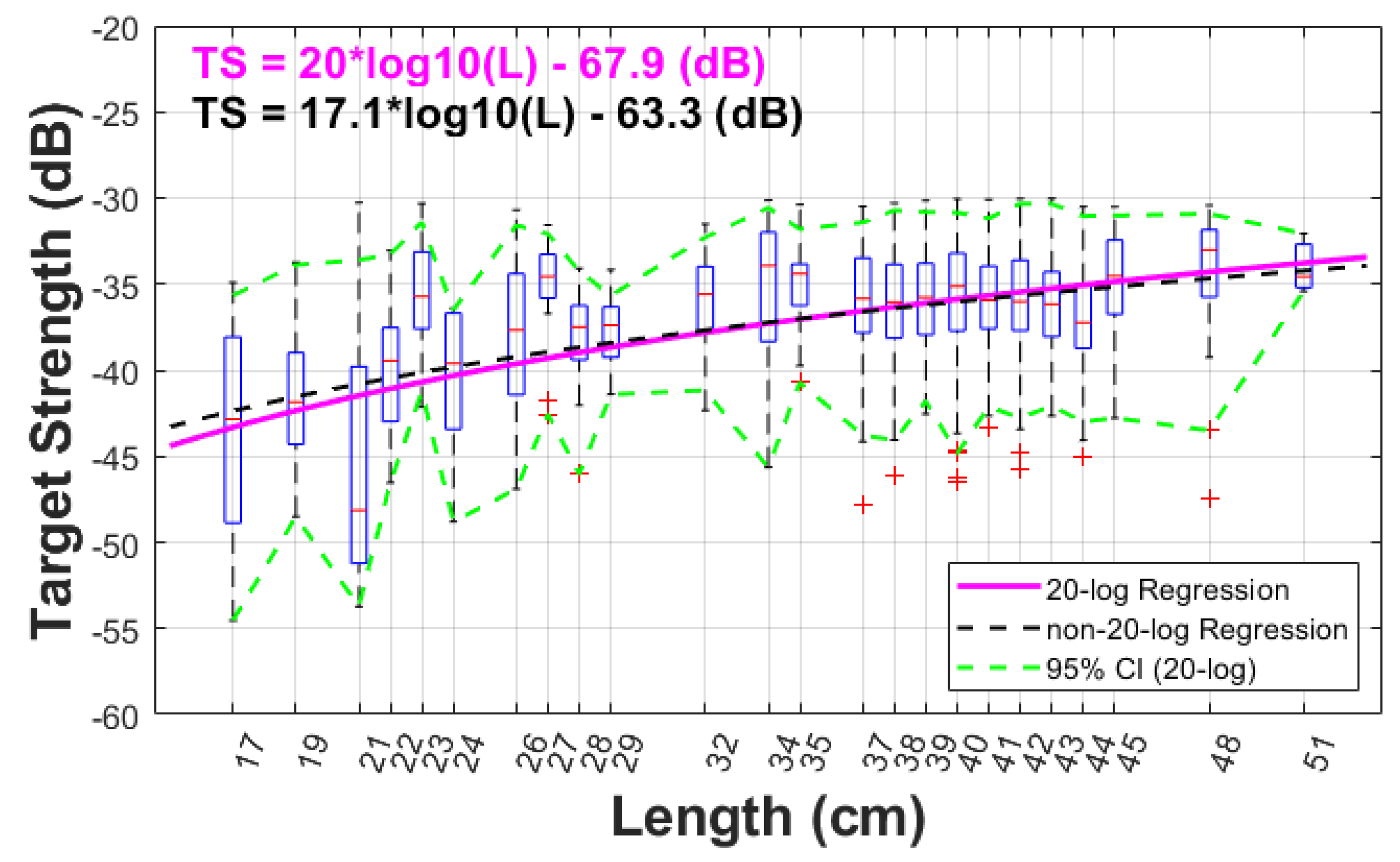
As a comparison, a linear regression where slope was estimated was also performed, resulting in a slope of 17.1 and the intercept of -63.3 dB. This regression curve is also shown in Figure 8 (dashed black line), which is not very different from the 20-log regression curve (solid magenta line) and well within the samples confidence interval that includes the 20-log. This non-20-log regression relation was an empirical data fit comparison. For gadoids, which have large spheroid-shape swimbladders, the relationship is justified to follow a 20 log relationship (Lauffenburger et al, 2023). Scattering physics reveals that the differential backscattering cross section in the farfield (i.e., plane wave incidence) should be proportional to the squared length of the target of finite size (i.e., smaller than the first Fresnel zone) (Morse and Ingard, 1968; Simmonds and MacLennan, 2005; Stanton, 1988, 1989). There has been debates in the literature that the relationships of target strength to length does not always necessarily follow a 20 log regression (McClatchie et al., 1996, 2003), perhaps due to complexity in fish body types and swimbladder morphologies.
3.5. Statistical Robustness of
To assess the robustness and the variability of the value of in the TS-length regression, we performed the three statistical processes as described in Sec. 2.2, i.e., partial, Bootstrapping, and Jackknife resampling methods, all with 1,000 iterations.
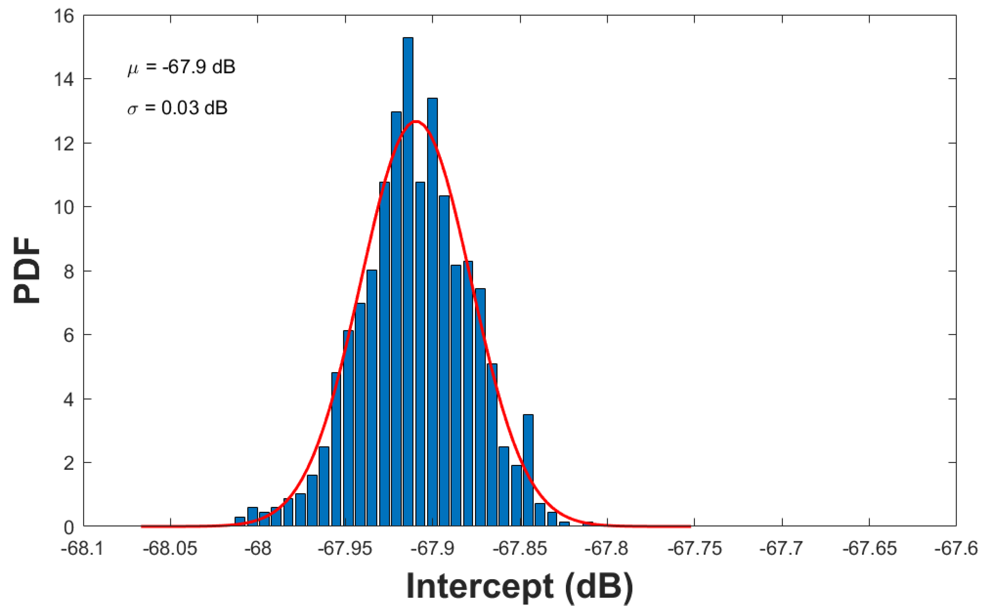
a. Partial sampling: For the partial sampling, we resampled the whole data population with 95% down to 5% in 5% increments, and at each percentage value we performed the resampling with replacement 1,000 times or realizations. The results are tabulated in Table 4 and their graphic representation is shown in Figure 9. All distributions from the resampling can be well described by Gaussian or Normal distributions. A representative example at 90% resampling is illustrated in Figure 10, where a Gaussian Probability Density Function (PDF) with a mean of -67.9 dB and standard deviation of 0.03 dB is superimposed onto the plot of the raw resampled values. Note that even with a substantially low number of selected TS samples at 5% of the original data, the estimated mean value of the in situ TS was only 0.003 dB lower than -67.9 dB.
b. Bootstrapping: Bootstrapping yielded a mean of -67.9 dB with a 95% confidence interval of [-68.09, -67.72]
c. Jackknife analysis also resulted in a mean of -67.9 dB with a standard deviation of 0.002 dB.
Table 4.
Results from the partial resampling with replacement.
| Resample Percentage | Mean (dB) | Standard Deviation (dB) |
|---|---|---|
| 5% | -67.9 | 0.42 |
| 10% | -67.9 | 0.29 |
| 20% | -67.9 | 0.19 |
| 30% | -67.9 | 0.15 |
| 40% | -67.9 | 0.12 |
| 50% | -67.9 | 0.10 |
| 60% | -67.9 | 0.08 |
| 70% | -67.9 | 0.06 |
| 80% | -67.9 | 0.05 |
| 85% | -67.9 | 0.04 |
| 90% | -67.9 | 0.03 |
| 95% | -67.9 | 0.02 |
These analyses all confirm the robustness of the estimate, with minimal variability, well within the tolerance uncertainty in the stock assessment (Grandin et al., 2024). The low variability observed in the data indicate consistency in TS measurements, likely the result of the extensive filtering of data, primarily based on the last step involving the pulse energy filter.
Figure 9.
estimates from Bootstrapping resampling with 5% to 95% of original TS samples, where 1,000 realizations were used.
Figure 9.
estimates from Bootstrapping resampling with 5% to 95% of original TS samples, where 1,000 realizations were used.
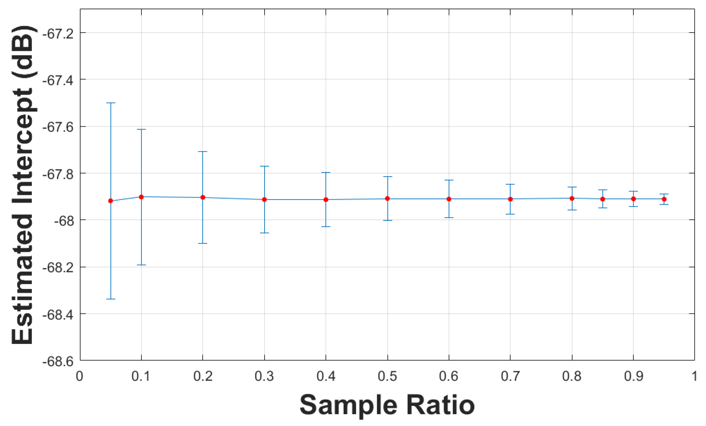
Figure 10.
estimate from partial resampling with 90% of the whole TS sample population, where 1,000 realizations were used. The parameters and are the mean and standard deviation of the Gaussian PDF (red solid line).
Figure 10.
estimate from partial resampling with 90% of the whole TS sample population, where 1,000 realizations were used. The parameters and are the mean and standard deviation of the Gaussian PDF (red solid line).
3.6. Comparison with Previous Studies
Although the value reported here is similar to that of Traynor (1996), it was 4–6 dB higher than that reported by Henderson and Horne (2007). Several factors may explain this discrepancy:
a. Data Collection Conditions: previous studies on Pacific hake used TS data collected at night, while all of the data presented in this paper were collected during daytime, i.e., consistent with the hake survey time from sunrise to sunset (Clemons et al., 2024). Hake TS measurements during daylight are more representative for biomass estimation as hake aggregates at depth during the day, but tend to scatter at night when there are less visual cues. As hake scatter and spread out through the water column at night they could present increased tilt angles, resulting in reduced TS values.
b. Length Range and Regression Consistency: Henderson and Horne’s ex situ TS data spanned a narrow fork length range (44–53 cm), with TS values spread over an 8 dB range (Figure 8 in Henderson and Horne, 2007), potentially reducing regression reliability and robustness.
c. Backscatter Model Discrepancies: The Kirchhoff Ray-Mode (KRM, Clay and Horne, 1994) backscatter model used by Henderson and Horne, with X-ray images of fish bodies and the swimbladders of live fish captured at sea, showed predictions 4–6 dB higher than their ex situ TS measurements (Fig. 6a in Henderson and Horne, 2007), indicating inconsistencies between model predictions and the ex situ measurements, but consistent with the findings from this study.
Results from these in situ measurements are consistent with the findings of Traynor (1996) despite their relatively small dataset of target strength measurements. The intercept value of -67.9 dB is in line, but lower by ~2 dB than reported for other gadoids (Rose and Porter, 1996, Pedersen et al., 2011, Lauffenburger et al., 2023). Consistency and low variability in TS measurements values observed over nine surveys (spanning 10 years) provide confidence in the use of the -68 dB intercept value currently used for Pacific hake biomass estimates obtained from acoustic surveys.
3.7. Limitations of the Study
Collection of Pacific hake in situ target strength data during the day is problematic because these fish tend to aggregate at high densities in relatively deep waters (often mixed with other smaller mesopelagic scatterers), making collection of ship-based data prone to multiple target bias. Collection made at shorter range, for example using the DAISY system, partially addresses this issue, but are resource demanding (requiring dedicated time and equipment). On the other hand, data collected during assessment and research surveys provide large volumes of data that can be mined afterward (see Lauffenburger et al., 2023 for another example). Because of the low signal to noise ratio conditions encountered in Pacific hake aggregations, selection of targets based on fish or target density metrics (Sawada et al. 1993, Gauthier and Rose, 2001), even at reduced survey speeds, were not used in this study (as very little data would be preserved). Rather, a stepwise approach to selection of targets was adopted, with the addition of a novel filter based on pulse energy used on the final dataset. The consistency of TS values obtained (especially when compared to closer measurements made with DAISY) provide further evidence for the validity of this approach. It is also important to note that ship-based target strength measurements in this study were all made during midwater trawling operations (because of the reduced vessel speed). There is evidence that trawling affect fish behavior (Winger et al., 2010). Acoustic data collection from the centerboard of the vessel were made prior to the trawl going through the aggregation, but increased vessel and trawling gear noise may have an impact on the orientation and swimming behavior of fish. There is however little evidence of change in aggregation characteristics and depth distribution prior compared to during trawling, so we are assuming that these measurements of target strength data were made on fish representative of those encountered during routine acoustic surveys.
4. Conclusion
Single-fish TS data of Pacific hake at 38 kHz from more than ten surveys and research cruises spanning ten years were analyzed. These data were processed with a number of filters and criteria to ensure data quality so that all accepted TS samples were expected to be from individual hake. All echosounder data sets were verified by biological trawl catches with an average hake composition of more than 95% by weight to ensure the echoes were most likely from hake. The TS-length regression of 20-log linear representation, i.e., Eq. (1), suggests an intercept term, of -67.9 dB, only 0.1 dB larger than the value currently used in acoustic biomass estimates. The updated aligns closely with current biomass estimation practices, ensuring accuracy well within acceptable uncertainty limits. The results from three statistical validation methods, i.e., partial, Bootstrapping, and Jackknife resampling procedures, were used to assess the variability of the estimated , ensuring accuracy within acceptable uncertainty limits while addressing discrepancies with earlier studies. These findings emphasize the importance of standardized sampling protocols and robust methods for advancing acoustic biomass assessment.
Acknowledgments
This project was supported by NOAA Fisheries and DFO. We acknowledge Chelsea Stanley and George Cronkite for their assistance with DAISY. Other members of the Fisheries Engineering and Acoustic Technologies team (NOAA/NWFSC) and DFO, Alicia Billings, John Pohl, Larry Hufnagle, Elizabeth Phillips, and Christopher Grandin helped in acoustic and biological data collections.
Table A1.
Detailed catch information of all hauls used in this study.
| Year | Haul Number | Latitude (deg North) | Longitude (deg West) | Mean fork length (cm) | Standard Deviation of fork length (cm) | CV (%) | # of length samples | Total catch (kg) | % of hake by weight | ||||||||||
|---|---|---|---|---|---|---|---|---|---|---|---|---|---|---|---|---|---|---|---|
| Shimada | |||||||||||||||||||
| 2009 | 8 | 37.0401 | 122.6764 | 40 | 3.76 | 9.4% | 324 | 321 | 95% | ||||||||||
| 2009 | 22 | 39.0280 | 123.9685 | 40 | 2.58 | 6.5% | 347 | 1,426 | 100% | ||||||||||
| 2009 | 39 | 42.7018 | 124.7260 | 38 | 2.34 | 6.2% | 437 | 4,590 | 100% | ||||||||||
| 2009 | 56 | 44.2032 | 124.9930 | 42 | 2.12 | 5.0% | 301 | 1,100 | 99% | ||||||||||
| 2009 | 57 | 44.3706 | 124.8315 | 41 | 2.5 | 6.1% | 288 | 446 | 100% | ||||||||||
| 2009 | 62 | 44.8783 | 124.4680 | 19 | 1.64 | 8.6% | 336 | 1,749 | 100% | ||||||||||
| 2009 | 64 | 44.8796 | 124.8209 | 43 | 2.52 | 5.9% | 248 | 128 | 99% | ||||||||||
| 2009 | 66 | 45.3749 | 124.4020 | 41 | 2.48 | 6.0% | 339 | 268 | 100% | ||||||||||
| 2011 | 2 | 35.3790 | 121.0993 | 22 | 1.25 | 5.7% | 242 | 82 | 99% | ||||||||||
| 2011 | 4 | 35.7137 | 121.4605 | 23 | 1.13 | 4.9% | 280 | 941 | 100% | ||||||||||
| 2011 | 9 | 37.3658 | 122.9050 | 24 | 1.88 | 7.8% | 208 | 18 | 100% | ||||||||||
| 2011 | 18 | 39.3728 | 123.9755 | 35 | 2.00 | 5.7% | 276 | 116 | 100% | ||||||||||
| 2011 | 27 | 44.3747 | 124.8392 | 39 | 2.96 | 7.6% | 307 | 216 | 99% | ||||||||||
| 2011 | 40 | 46.8773 | 124.9192 | 37 | 1.83 | 5.0% | 264 | 259 | 100% | ||||||||||
| 2011 | 44 | 47.3707 | 124.8633 | 38 | 1.93 | 5.1% | 325 | 140 | 100% | ||||||||||
| 2013 | 5 | 35.4248 | 121.3085 | 35 | 1.00 | 2.9% | 118 | 33 | 99% | ||||||||||
| 2013 | 10 | 35.9212 | 121.5310 | 26 | 1.42 | 5.5% | 317 | 463 | 100% | ||||||||||
| 2013 | 13 | 36.5982 | 122.6653 | 37 | 1.56 | 4.2% | 308 | 181 | 100% | ||||||||||
| 2013 | 16 | 37.2632 | 123.0873 | 37 | 1.72 | 4.7% | 536 | 177 | 99% | ||||||||||
| 2013 | 18 | 37.4207 | 122.9600 | 37 | 1.54 | 4.2% | 333 | 495 | 100% | ||||||||||
| 2013 | 33 | 40.5868 | 124.6773 | 38 | 2.24 | 5.9% | 556 | 198 | 98% | ||||||||||
| 2013 | 38 | 41.5960 | 124.5763 | 37 | 1.56 | 4.2% | 414 | 369 | 100% | ||||||||||
| 2013 | 42 | 43.0928 | 124.8732 | 37 | 1.94 | 5.2% | 397 | 259 | 98% | ||||||||||
| 2013 | 45 | 43.9313 | 124.9667 | 38 | 2.15 | 5.7% | 345 | 446 | 100% | ||||||||||
| 2013 | 48 | 44.2608 | 124.9428 | 39 | 2.69 | 6.9% | 230 | 86 | 100% | ||||||||||
| 2013 | 56 | 46.2453 | 124.2052 | 40 | 2.97 | 7.4% | 353 | 318 | 97% | ||||||||||
| 2013 | 76 | 50.0928 | 128.0172 | 51 | 3.62 | 7.1% | 537 | 522 | 89% | ||||||||||
| 2014 | 15 | 43.8840 | 124.7910 | 43 | 3.16 | 7.3% | 237 | 642 | 100% | ||||||||||
| 2014 | 16 | 43.8858 | 124.7343 | 44 | 3.35 | 7.6% | 200 | 192 | 100% | ||||||||||
| 2015 | 9 | 36.4460 | 122.1363 | 23 | 2.22 | 9.7% | 373 | 49 | 98% | ||||||||||
| 2015 | 13 | 37.4495 | 122.9712 | 22 | 1.46 | 6.6% | 285 | 431 | 88% | ||||||||||
| 2015 | 15 | 38.1177 | 123.6143 | 24 | 1.06 | 4.4% | 375 | 69 | 94% | ||||||||||
| 2015 | 21 | 39.7728 | 124.0748 | 35 | 3.40 | 9.7% | 418 | 166 | 100% | ||||||||||
| 2015 | 39 | 43.4477 | 124.7072 | 24 | 1.36 | 5.7% | 323 | 1,316 | 100% | ||||||||||
| 2015 | 42 | 43.7828 | 124.9052 | 42 | 1.56 | 3.7% | 62 | 34 | 96% | ||||||||||
| 2015 | 46 | 44.7827 | 124.6060 | 21 | 1.23 | 5.9% | 481 | 290 | 100% | ||||||||||
| 2015 | 60 | 47.3663 | 124.8485 | 23 | 2.02 | 8.8% | 237 | 314 | 99% | ||||||||||
| 2015 | 73 | 49.1188 | 126.8678 | 44 | 2.37 | 5.4% | 288 | 156 | 100% | ||||||||||
| 2016 Winter | 2 | 42.1750 | 124.6632 | 29 | 2.74 | 9.4% | 235 | 35 | 92% | ||||||||||
| 2016 Winter | 4 | 41.3485 | 124.4978 | 27 | 1.58 | 5.9% | 474 | 440 | 93% | ||||||||||
| 2016 Winter | 7 | 41.4722 | 125.0988 | 44 | 2.72 | 6.2% | 195 | 234 | 96% | ||||||||||
| 2016 Winter | 8 | 40.4218 | 125.0995 | 44 | 3.04 | 6.9% | 221 | 460 | 100% | ||||||||||
| 2016 Winter | 9 | 39.8428 | 125.0960 | 44 | 3.02 | 6.9% | 123 | 61 | 97% | ||||||||||
| 2016 Winter | 10 | 39.1192 | 125.2397 | 43 | 2.55 | 5.9% | 256 | 141 | 85% | ||||||||||
| 2016 Winter | 11 | 39.1202 | 125.2287 | 43 | 2.59 | 6.0% | 256 | 118 | 99% | ||||||||||
| 2016 Winter | 13 | 37.9578 | 123.5278 | 28 | 1.67 | 6.0% | 210 | 125 | 96% | ||||||||||
| 2016 Winter | 18 | 37.2152 | 124.0930 | 42 | 3.01 | 7.2% | 211 | 237 | 100% | ||||||||||
| 2016 Winter | 21 | 35.9870 | 123.8852 | 43 | 2.43 | 5.7% | 235 | 139 | 92% | ||||||||||
| 2016 Winter | 29 | 37.1723 | 124.0630 | 42 | 2.99 | 7.1% | 231 | 332 | 98% | ||||||||||
| 2016 Winter | 30 | 39.0515 | 125.1992 | 42 | 3.00 | 7.1% | 200 | 225 | 99% | ||||||||||
| 2016 Winter | 32 | 42.5568 | 125.8293 | 44 | 2.75 | 6.3% | 287 | 143 | 97% | ||||||||||
| 2017 Summer | 1 | 34.9915 | 121.0798 | 26 | 2.14 | 8.2% | 331 | 37 | 98% | ||||||||||
| 2017 Summer | 4 | 36.4908 | 122.1897 | 28 | 2.15 | 7.7% | 415 | 1,163 | 98% | ||||||||||
| 2017 Summer | 10 | 38.3297 | 123.6627 | 37 | 2.39 | 6.5% | 395 | 531 | 98% | ||||||||||
| 2017 Summer | 14 | 39.1445 | 124.0088 | 38 | 2.30 | 6.1% | 403 | 351 | 95% | ||||||||||
| 2017 Summer | 16 | 40.8132 | 124.5613 | 40 | 2.90 | 7.3% | 419 | 316 | 91% | ||||||||||
| 2017 Summer | 19 | 41.6540 | 124.4612 | 27 | 1.91 | 7.1% | 250 | 90 | 99% | ||||||||||
| 2017 Summer | 20 | 41.8235 | 124.4860 | 28 | 1.87 | 6.7% | 242 | 586 | 100% | ||||||||||
| 2017 Summer | 25 | 42.9898 | 125.1188 | 41 | 2.92 | 7.1% | 226 | 119 | 95% | ||||||||||
| 2017 Summer | 31 | 44.1580 | 124.9715 | 39 | 2.76 | 7.1% | 396 | 202 | 98% | ||||||||||
| 2017 Winter | 3 | 42.1720 | 124.5940 | 19 | 1.28 | 6.7% | 156 | 51 | 96% | ||||||||||
| 2017 Winter | 4 | 37.2585 | 123.3062 | 35 | 2.22 | 6.3% | 201 | 123 | 93% | ||||||||||
| 2017 Winter | 6 | 35.4527 | 123.5482 | 43 | 3.21 | 7.5% | 191 | 99 | 100% | ||||||||||
| 2017 Winter | 7 | 34.4397 | 120.7680 | 21 | 1.07 | 5.1% | 401 | 100 | 100% | ||||||||||
| 2017 Winter | 12 | 38.9510 | 124.0153 | 34 | 1.67 | 4.9% | 301 | 1,080 | 100% | ||||||||||
| 2018 | 18 | 44.5778 | 124.6725 | 41 | 2.81 | 6.9% | 245 | 378 | 100% | ||||||||||
| 2018 | 19 | 44.5685 | 124.6752 | 43 | 2.67 | 6.2% | 236 | 156 | 97% | ||||||||||
| 2019 | 7 | 35.3937 | 121.1582 | 22 | 1.26 | 5.7% | 212 | 52 | 100% | ||||||||||
| 2019 | 8 | 35.5583 | 121.4342 | 23 | 1.69 | 7.3% | 212 | 104 | 99% | ||||||||||
| 2019 | 12 | 36.0648 | 121.7403 | 24 | 2.44 | 10.2% | 220 | 87 | 97% | ||||||||||
| 2019 | 19 | 37.5640 | 123.0483 | 32 | 2.32 | 7.3% | 356 | 178 | 100% | ||||||||||
| 2019 | 22 | 38.0565 | 123.5303 | 42 | 3.70 | 8.8% | 349 | 525 | 99% | ||||||||||
| 2019 | 24 | 38.5600 | 123.7883 | 38 | 3.01 | 7.9% | 322 | 121 | 94% | ||||||||||
| 2019 | 25 | 38.7320 | 123.8278 | 39 | 3.17 | 8.1% | 334 | 141 | 100% | ||||||||||
| 2019 | 29 | 39.4012 | 123.9842 | 40 | 2.25 | 5.6% | 326 | 182 | 92% | ||||||||||
| 2019 | 30 | 39.7312 | 124.2135 | 41 | 2.22 | 5.4% | 441 | 210 | 98% | ||||||||||
| 2019 | 33 | 40.3948 | 124.7948 | 41 | 2.07 | 5.0% | 403 | 413 | 100% | ||||||||||
| 2019 | 35 | 40.5643 | 124.7252 | 41 | 2.68 | 6.5% | 438 | 612 | 99% | ||||||||||
| 2019 | 36 | 40.7295 | 124.8352 | 41 | 2.57 | 6.3% | 468 | 648 | 100% | ||||||||||
| 2019 | 38 | 41.0465 | 124.4185 | 42 | 2.83 | 6.7% | 373 | 393 | 100% | ||||||||||
| 2019 | 45 | 42.7263 | 124.7283 | 42 | 3.23 | 7.7% | 381 | 1,567 | 100% | ||||||||||
| 2019 | 46 | 42.8943 | 124.9795 | 42 | 2.99 | 7.1% | 366 | 576 | 100% | ||||||||||
| 2019 | 47 | 43.0708 | 125.0855 | 42 | 2.54 | 6.0% | 235 | 115 | 97% | ||||||||||
| 2019 | 48 | 43.2257 | 124.7650 | 42 | 2.47 | 5.9% | 343 | 313 | 100% | ||||||||||
| 2019 | 50 | 43.7210 | 125.0668 | 43 | 2.44 | 5.7% | 215 | 111 | 100% | ||||||||||
| 2019 | 54 | 44.0552 | 124.9563 | 41 | 2.73 | 6.7% | 381 | 701 | 99% | ||||||||||
| 2019 | 56 | 45.0540 | 124.7597 | 44 | 1.97 | 4.5% | 83 | 46 | 97% | ||||||||||
| 2019 | 57 | 45.2223 | 124.6620 | 43 | 2.02 | 4.7% | 276 | 148 | 97% | ||||||||||
| 2019 | 59 | 45.5570 | 124.5612 | 45 | 2.12 | 4.7% | 184 | 107 | 97% | ||||||||||
| DAISY | |||||||||||||||||||
| 9/7/2014 | 36 | 41.6582 | 124.5003 | 29 | 1.25 | 4.3% | 101 | 259 | 80% | ||||||||||
| 9/12/2014 | 41 | 48.9242 | 126.5505 | 48 | 3.41 | 7.1% | 174 | 161 | 82% | ||||||||||
| 3/23/2016 | 30 | 50.0170 | 123.9078 | 33 | 4.70 | 14.2% | 150 | 29 | 99% | ||||||||||
| Mean | 41.0717 | 124.1269 | 36.2 | 2.34 | 6.5% | 299 | 379 | 98% | |||||||||||
References
- Blackman, S. S., 1986. Multiple-target tracking with radar applications. Artech House.
- Chu. D., 2024. Development and Application of Advanced Science and Technology in Fisheries Acoustics. J. Marine Acoust. Soc. Jpn. 51(4): 117-149.
- Clay, C. S., and Horne, J. K., 1994. Acoustic models of fish: The Atlantic cod (Gadus morhua). J. Acoust. Soc. Am. 96: 1661–1668. [CrossRef]
- Clemons, J. E., S. Gauthier, S. K. de Blois, A. A. Billings, E. M. Phillips, J. E. Pohl, C. P. Stanley, R. E. Thomas and E. M. Beyer. 2024. The 2023 Joint U.S.–Canada Integrated Ecosystem and Pacific Hake Acoustic Trawl Survey: Cruise Report SH-23-06. U.S. Department of Commerce, NOAA Processed Report NMFS-NWFSC-PR-2024-01.
- Demer, D. A., Andersen, L. N., Bassett, C., Berger, L., Chu, D., Condiotty, J., Cutter, G. R., et al. 2017. 2016 USA–Norway EK80 Workshop Report: Evaluation of a wideband echosounder for fisheries and marine ecosystem science. ICES Cooperative Research Report No. 336. 69 pp. [CrossRef]
- Efron, B. and Tibshirani, R.,1993. An Introduction to the Bootstrap. Boca Raton, FL: Chapman & Hall/CRC. ISBN 0-412-04231-2.
- Efron, B. , 2003. Second thoughts on the bootstrap (PDF). Statistical Science. 18(2): 135–140. [CrossRef]
- Fleischer, G. W. , Cooke, K. D., Ressler, P. H., Thomas, R. E., de Blois, S. K., Hufnagle, L. C., Kronlund, A. R., Holmes, J. A., and Wilson, C. D., 2005. The 2003 integrated acoustic and trawl survey of Pacific hake, Merluccius productus, in U.S. and Canadian waters off the Pacific coast. U.S. Department of Commerce, NOAA Technical Memorandum NMFS-NWFSC-65.
- Foote, K. G. , 1985. Rather-high-frequency sound scattering by swimbladdered fish. J. Acoust. Soc. Am., 78: 688–700. [CrossRef]
- Gauthier, S. and Rose, G.A., 2002. In situ target strength studies on Atlantic redfish (Sebastes spp.). ICES J. Mar. Sci., 59: 805-815. [CrossRef]
- Grandin, C. J. , Johnson, K. F., Edwards, A. M., Berger, A. M., 2024. Status of the Pacific Hake (whiting) stock in U.S. and Canadian waters in 2024. Prepared by the Joint Technical Committee of the U.S. and Canada Pacific Hake/Whiting Agreement, National Marine Fisheries Service and Fisheries and Oceans Canada. 246 p.
- Henderson, M. J. and Horne, J. K., 2007. Comparison of in situ, ex situ, and backscatter model estimates of Pacific hake (Merluccius productus) target strength. Can. J. Fish. Aquat. Sci. 64: 1781-1794. [CrossRef]
- Horowitz, J. L. , 2019. Bootstrap methods in econometrics. Annual Review of Economics. 11: 193–224.
- Jones, H. L. , 1974. Jackknife estimation of functions of stratum mean. Biometrika. 61: 343–348. [CrossRef]
- Johnson, K.F., A.M. Edwards, A.M. Berger, and C.J. Grandin, 2021. Status of the Pacific Hake (whiting) stock in U.S. and Canadian waters in 2021. Prepared by the Joint Technical Committee of the U.S. and Canada Pacific Hake/Whiting Agreement, National Marine Fisheries Service and Fisheries and Oceans Canada.
- Kloser, R. J., Ryan, T. E., Macaulay, G. J., and Lewis, M. E., 2011. In situ measurements of target strength with optical and model verification: a case study for blue grenadier, Macruronus novaezelandiae. 68: 1986-1995. [CrossRef]
- Lauffenburger, N. , De Robertis, A., and Williams, K. 2023. Mining previous acoustic surveys to improve walleye pollock (Gadus chalcogrammus) target strength estimates. ICES Journal of Marine Science, 0: 1–14. [CrossRef]
- Longo, G.C., Head, M., Parker-Stetter, S., Taylor, I., Tuttle, V., Billings, A., Gauthier, S., McClure, M., Nichols, K.M. 2024. Population genomics of coastal Pacific Hake (Merluccius productus). North American Journal of Fisheries Management, 44:222–234. [CrossRef]
- Love, R. H. , 1978. Resonant acoustic scattering by swimbladder-bearing fish. J. Acoust. Soc. Am. 64: 571–580. [CrossRef]
- McClatchie, S. , Alsop, J., and Coombs, R. F. 1996. A re-evaluation of relationships between fish size, acoustic frequency and target strength. ICES Journal of Marine Science, 53: 780–791. [CrossRef]
- McClatchie, S. , Macaulay, G. J., and Coombs, R. F. 2003. A requiem for the use of 20 log(10) length for acoustic target strength with special reference to deep-sea fishes. ICES Journal of Marine Science, 60: 419–428. [CrossRef]
- Madirolas, A. , Membiela, F. A., Gonzalez, J. D., Cabreira, A. G., dell’Erba, M., Prario, I. S., and Blanc, S., 2017. Acoustic target strength (TS) of argentine anchovy (Engraulis anchoita): the nighttime scattering layer. ICES J. Mar. Sci., 74: 1408–1420. [CrossRef]
- Medwin, H. and Clay, C. S., 1998. Fundamentals of Acoustic Oceanography, Academic Press. [CrossRef]
- Morse, P. H. and Ingard, U., 1968. Theoretical Acoustics. McGraw-Hill, New York.
- Ona, E. (ed), 1999. Methodology for Target Strength Measurements (With special reference to in situ techniques for fish and mikro-nekton). ICES Cooperative Research Report No. 235. 59 pp.
- Pedersen, G. Godø, O. R., Ona, E. and Macaulay, G. J. 2011. A revised target strength–length estimate for blue whiting (Micromesistius poutassou): implications for biomass estimates, ICES Journal of Marine Science, Volume 68 (10): 2222–2228. [CrossRef]
- Peña, H., 2008. In situ target-strength measurements of Chilean jack mackerel (Trachurus symmetricus murphyi) collected with a scientific echosounder installed on a fishing vessel. ICES J. Mar. Sci., 65: 594-604. [CrossRef]
- Rose, G. A. and Porter, D. R. 1996. Target-strength studies on Atlantic cod (Gadus morhua) in Newfoundland waters, ICES Journal of Marine Science, Volume 53 (2): 259–265. [CrossRef]
- Simmonds, J. and MacLennan, D.N., 2005. Fisheries Acoustics: Theory and Practice. 2nd Ed. Blackwell Publishing, London. ISBN 978-0-632-05994-2.
- Scherbino, M. and Truskanov, M. D., 1966. Determination of fish concentration by means of acoustic apparatus. ICES CM 1966/F:3, p. 6.
- Stanton, T. K. , 1988. Sound scattering by cylinders of finite length. I. Fluid cylinders, J. Acoust. Soc. Am., 83: 55-63. [CrossRef]
- Stanton, T.K. , (1989) Sound scattering by cylinders of finite length. III. Deformed, J. Acoust. Soc. Am., 86: 691-705. [CrossRef]
- Traynor, J. J. , 1996. Target-strength measurements of walleye pollock (Theragra chalcogramma) and Pacific whiting (Merluccius productus). ICES J. Mar. Sci. 53:253-258. [CrossRef]
- Winger, P.D. , Eayrs, S. and Glass, C.W. 2010. Fish Behavior near Bottom Trawls. In Behavior of Marine Fishes, P. He (Ed.). [CrossRef]
Figure 1.
Survey area map and the locations of the biological trawls associated with the TS samples from individual hake used in this study (circles for summer trawls, triangles for winter trawls). The survey transects are for the actual 2019 hake survey and the inset is the photo of the DAISY deployed off the Canadian Coast Guard Ship (CCGS) W. E. Ricker.
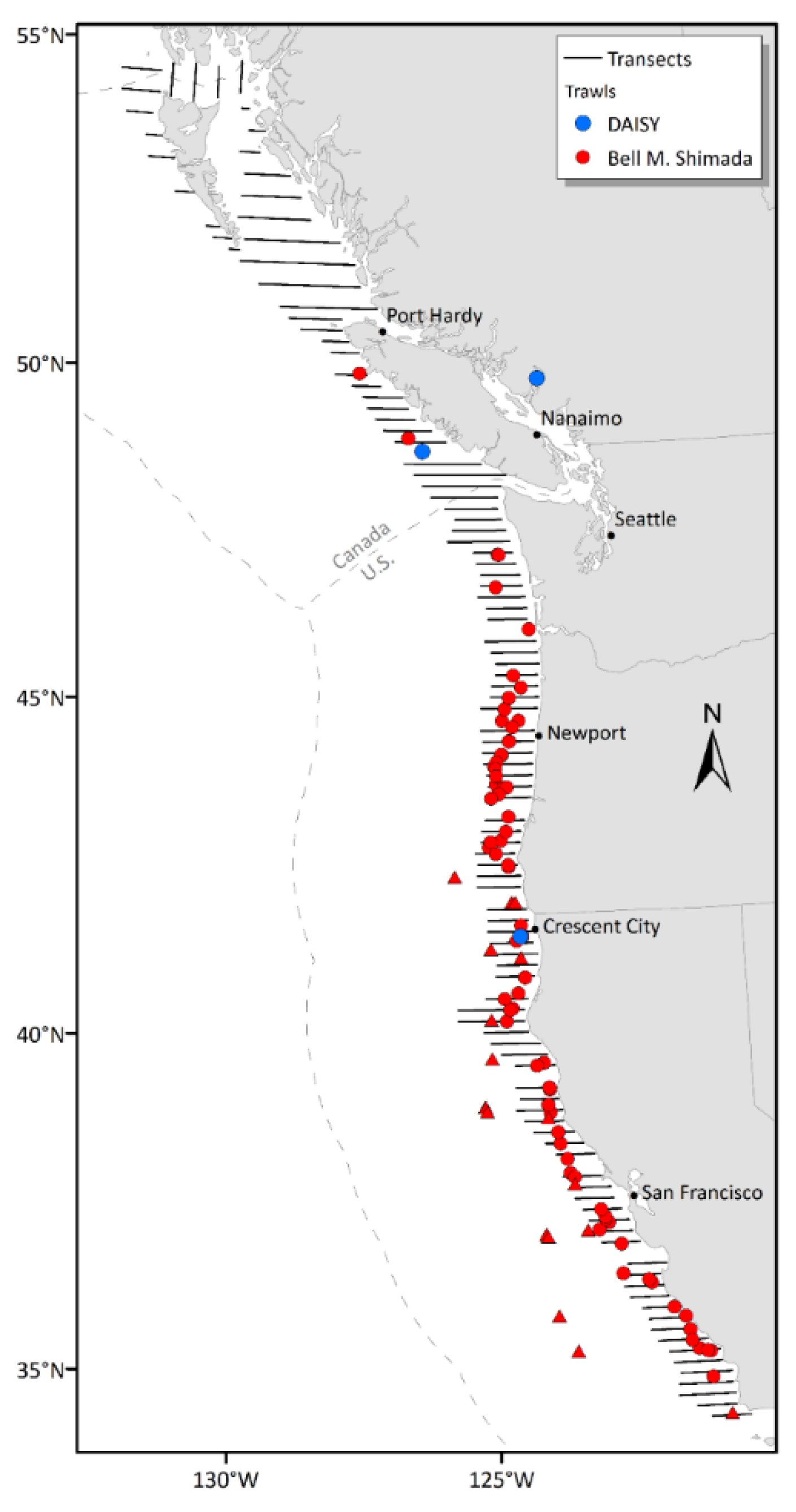
Figure 3.
Histogram of the TS from single targets.
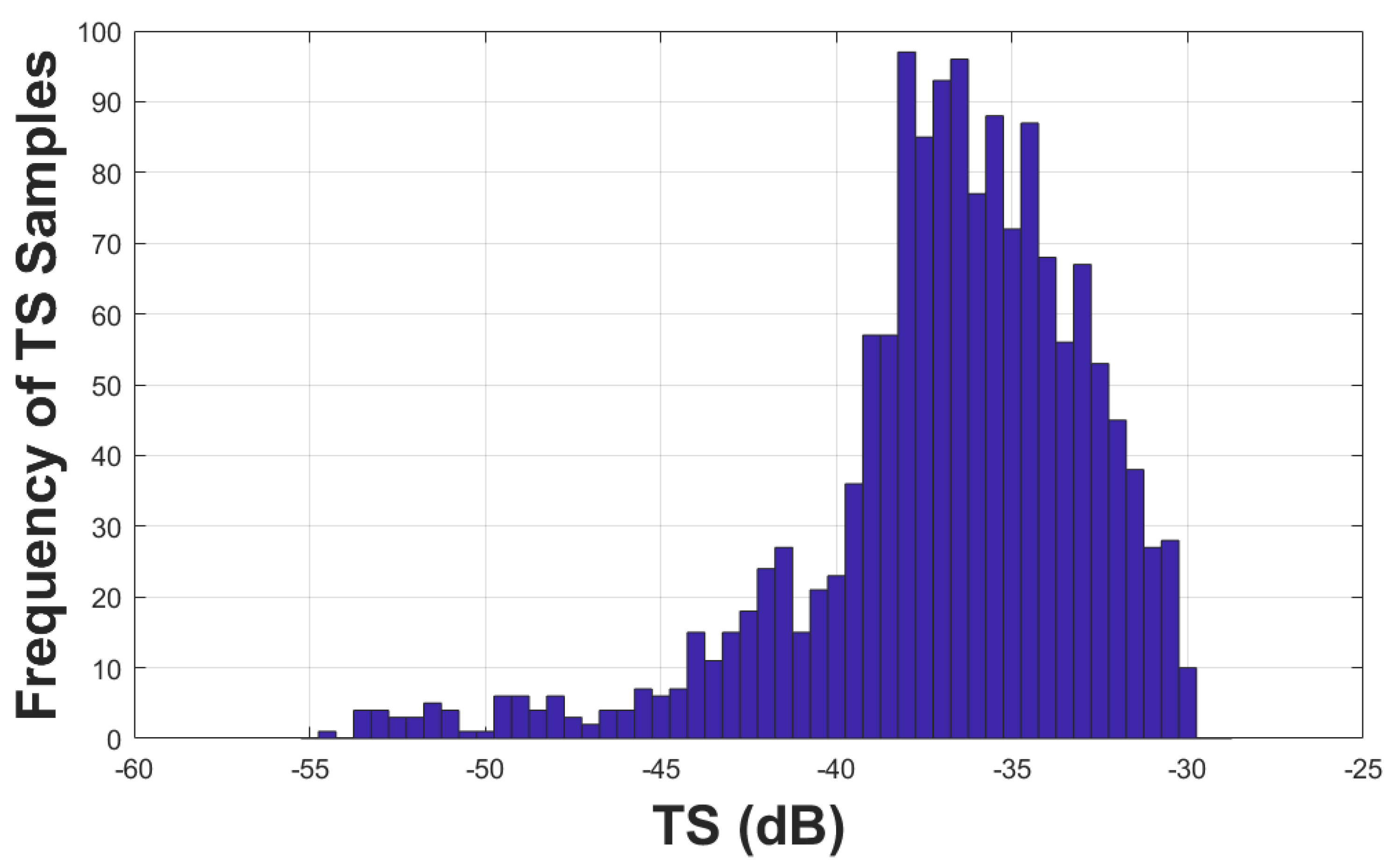
Figure 4.
Histogram of the TS from single targets as a function of target depth.
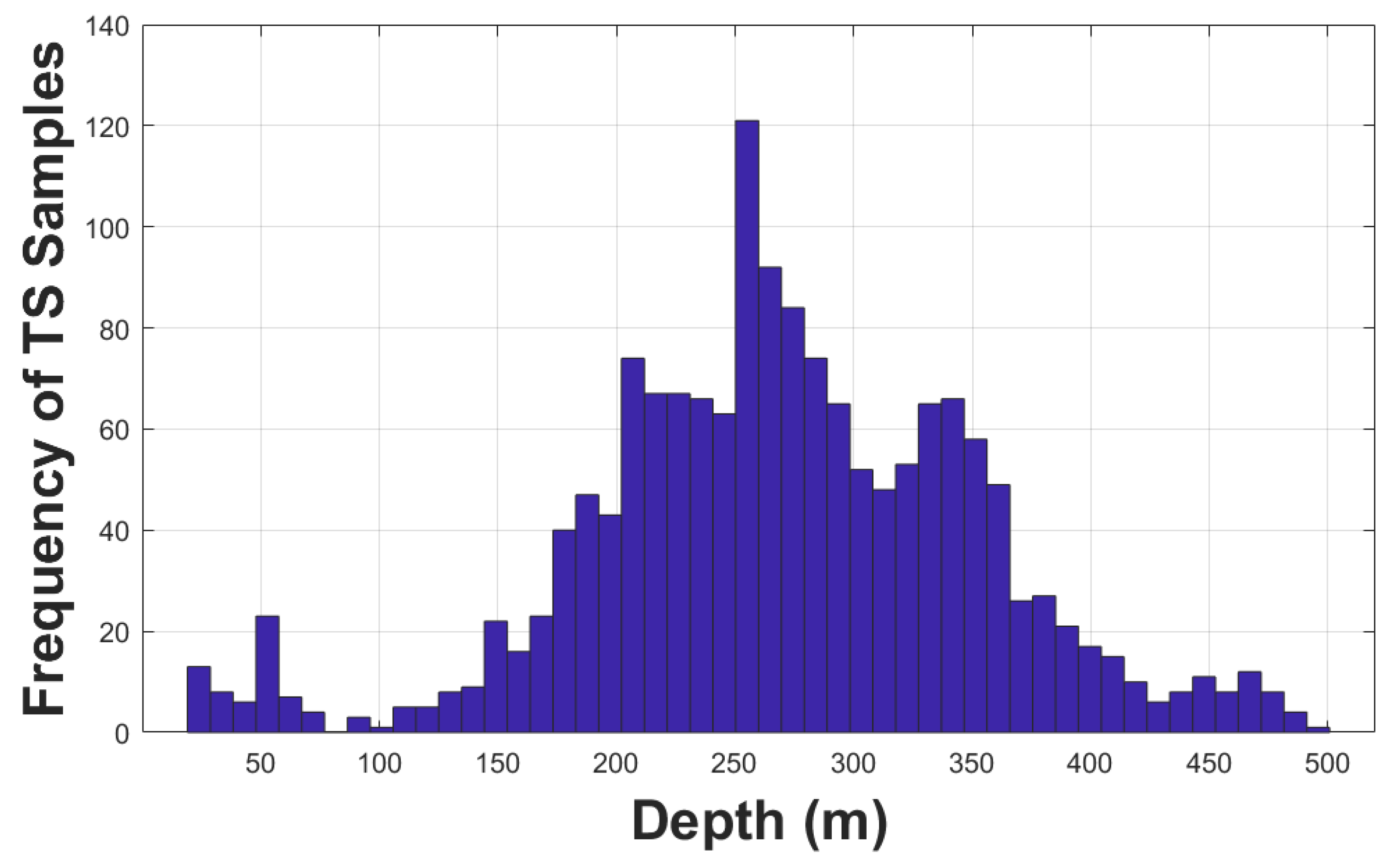
Figure 5.
Target strength (TS) from single targets as a function of depth, where the central mark (red line) is the median, the edges of the box (blue) are the 25th and 75th percentiles, the whiskers (black dashed line) extend to the most extreme data points (red plus) that the algorithm considers to be not outliers, and these outliers are plotted individually.
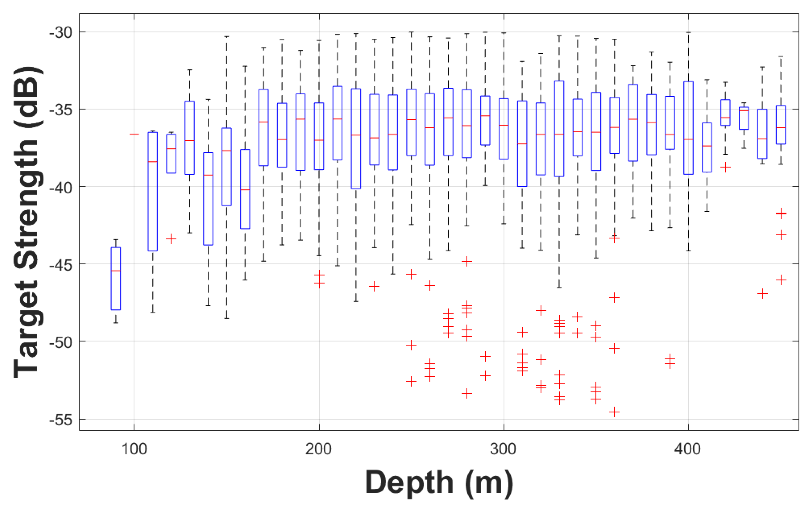
Figure 6.
Target strength (TS) from single targets as a function of latitude.
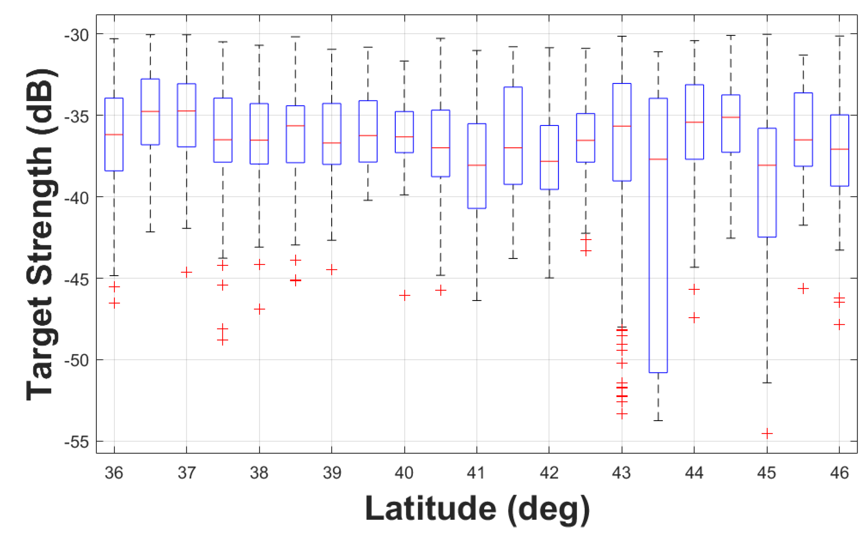
Figure 7.
Hake fork length from biological haul catches as a function of length.
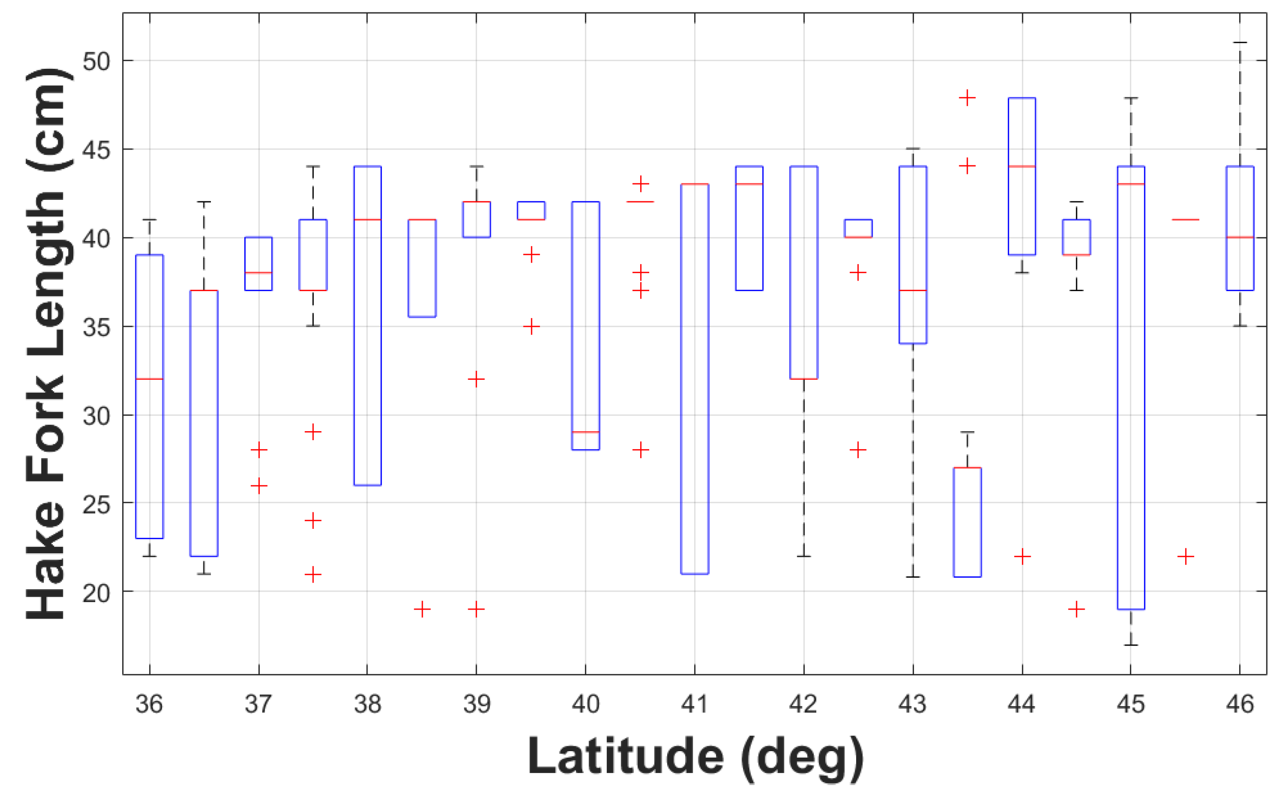
Table 3.
Information of target strength (TS) samples from the targets associated with the chosen midwater trawl hauls. The average catch weight per haul was 377 kg and the average hake catch was 97%.
Table 3.
Information of target strength (TS) samples from the targets associated with the chosen midwater trawl hauls. The average catch weight per haul was 377 kg and the average hake catch was 97%.
| Dataset | No. Hauls | TS Samples (original) | TS Samples (Pulse-energy filtered') |
|---|---|---|---|
| 2009 | 8 | 6891 | 150 |
| 2011 | 7 | 4875 | 98 |
| 2013 | 12 | 14103 | 241 |
| 2014 | 2 | 1898 | 6 |
| 2015 | 9 | 1915 | 48 |
| 2016 Winter | 13 | 9922 | 218 |
| 2017 Winter | 9 | 4158 | 92 |
| 2017 Summer | 5 | 3365 | 61 |
| 2018 | 2 | 216 | 5 |
| 2019 | 22 | 16829 | 481 |
| DAISY 2014-09-07 | 1 | 3722 | 40 |
| DAISY 2014-09-12 | 1 | 3788 | 47 |
| DAISY 2016-03-23 | 1 | 5372 | 23 |
| Sum | 92 | 77054 | 1510 |
Disclaimer/Publisher’s Note: The statements, opinions and data contained in all publications are solely those of the individual author(s) and contributor(s) and not of MDPI and/or the editor(s). MDPI and/or the editor(s) disclaim responsibility for any injury to people or property resulting from any ideas, methods, instructions or products referred to in the content. |
© 2025 by the authors. Licensee MDPI, Basel, Switzerland. This article is an open access article distributed under the terms and conditions of the Creative Commons Attribution (CC BY) license (https://creativecommons.org/licenses/by/4.0/).
Copyright: This open access article is published under a Creative Commons CC BY 4.0 license, which permit the free download, distribution, and reuse, provided that the author and preprint are cited in any reuse.


