
Submitted:
30 September 2025
Posted:
01 October 2025
You are already at the latest version
Abstract
Nowadays, birds damage to field crops such as corvids and pigeons has become crucial for many farmers. Damage can be as serious as the loss of a large part of the harvest. Several solutions have been proposed, but none is effective. For example, the use of scarecrows, but birds eventually adapt to them over time, and so they become ineffective. To study bird behavior and to propose a bird deterrent that would adapt to the presence of birds, we set up an experimental image-taking system on several plots of land over a period of 4-5 years. Around fifteen terabytes of images taken in the field have been acquired. Our aim is to automatically detect these birds using Deep Learning methods, and then to activate a real time scarer. This work meets two challenges: the first is agroecological, as bird damage has become a major issue, and the second is IT, as it is difficult to detect birds in the field: the individuals are small because they are far from the camera lens, and field conditions are often less than optimal: darkness, confusion between the pigeons' colors and the ground, etc. The Mask-RCNN in its original configuration is not suited to detecting small individuals. We have mainly focused on the model's hyperparameters to better adapt it to our study context. As a result, we have improved the detection of small individuals using, among other things, appropriate anchor scales design and image processing techniques. At the same time, we have built an original dataset focused on small individuals called Birdydataset. The model can detect corvids and pigeons with an accuracy of 78 % under real field conditions.
Keywords:
bird detection and identification
; deep learning
; agro-ecology
; IA-Mask-RCNN
1. Introduction
Bird damage at field crop establishment is a major problem for growers of certain crops such as corn and sunflower (Sausse et al., 2021a). Current protection methods are unsatisfactory. With the supply of repel-lent products dwindling due to their toxicity, farmers are resorting to the controversial method of bird kill-ing, or to scaring devices, especially with sound, that may be ineffective due to the birds’ habituation (Gilsdorf et al., 2002). Bird damage has a heavy-tailed distribution (Sausse et al. 2021b; Johnson et al., 1989): it affects few fields but is highly damaging and random. This implies preventive and systematic scaring strategies, which encourage conflicts with nearby residents and bird habituation. Furthermore, it makes it difficult for observers to study how birds frequent fields, which could provide us with knowledge prior to establish prevention strategies. In addition, these methods are generally time-consuming or lack precision.
Optical bird detection offers opportunities on both sides. Real-time analysis would make it possible to trigger a bird scaring device only when birds are present, or even to send an alert to the farmer. For re-search purposes, the detection of birds on the ground using vast banks of images from time lapse cameras would make it possible to establish precise patterns of field frequentation over time and space. More gen-erally, Bird Identification and Detection (BIAD) has become an important topic in the fields of computer visualization, acoustic sensing and artificial intelligence. Indeed, BIAD has a wide range of applications.
Work on BIAD has mainly been carried out in the context of building (e.g., Schiano et al., 2022) and airport protection (review from Fu et al., 2024), or endangered bird protection (e.g., Zhu et al., 2024). Research on agricultural applications concern on-board optical detection by UAVs in the case of rice (Yakubu and al., 2025) and ripening crops (Nirmala Devi et al., 2024). But to our knowledge, no work has been published for application to our case of birds landing in field crops at emergence with image acquisition by fixed horizontal shooting. This case presents specific difficulties. The fields to be monitored are large (4.38 ha for sunflower in France), which reduces the size of the objects to be detected. The background may be het-erogeneous, with bare soil of varying degrees of stoniness, and plants or weeds at emergence. Finally, damage can occur at dawn or dusk in variable lighting conditions and, of course, in different weather con-ditions.
Over the past 5 years, we acquired many images taken in the field on several plots, with a view to analyzing them using the latest image processing and deep learning methods. Our aim is to be able to detect the presence of birds in real time and thus scare them off at that precise moment. The aim is also to prevent birds getting used to these new scarecrows in the same way as the more conventional ones.
This paper presents an automatic method for detecting birds from raw field images. By detection we mean the location of individuals on the image and their classification, i.e., assigning them the correct class label. Our study focuses on corvids and pigeons, which cause a great deal of damage to field crops such as corn and sunflowers.
2. Related Works in Bird Identification and Detection (BIAD)
The most advanced methods for detecting and classifying individuals are based on Neural Convolution Networks (CNN), in particular the Region Convolutional Neural Network (RCNN) (Girshick, 2015, Ren, 2016). Among the RCNN we have chosen the Mask-RCNN (He, 2018) which combines the latest advances in the fields of neural networks and computer vision. The Mask-RCNN is a two-pass CNN model. On the other hand, there is one pass model for detecting individuals in real time, which is faster but less accurate than double-pass models. YOLO (You Only Look Once) by simultaneously detecting and classifying objects in one pass, has made it possible to combine real-time speed with precision. YOLO was introduced by (Redmon and al, 2015). and has since undergone several iterations, the latest being YOLOv12. Recently, (Haitong and al., 2023), (Lou and al. 2023) proposed DC-YOLOv8, a small-size Object Detection Algorithm (ODA) based on camera sensor for special scenarios. Their results show that the mAP (mean Average Precision) rises from 39% for YOLO to 41.5% for DC-YOLO. So, these scores remain rather modest compared with the challenges of real-time detection of small objects. YOLO has also been used in an agricultural and environmental context for smoke and fire detection (Ramos et al., 2024). To do this, the authors attempted to optimize the model’s hyperparameters, obtaining results with accuracy and recall greater than 1.39% and 1.48%, respectively.
Regarding bird detection, YOLO has been used in the field (Félix-Jiménez et al., 2025). However, in this latest study, the recommended exposure distance for individuals facing the camera is 3 meters, with a maximum of 5 meters. Our study focuses on the presence of birds in real plots; this distance could be 100 meters or more. It should be noted that the majority of BIADs are based on Yolo or its improvement for reasons of simplicity and real-time performance.
While Mask-RCNN, in its default parameters configuration, performs well with large objects, when individuals are clearly visible in the image, occupying a good proportion of it, the same cannot be said for detecting small objects or at a distance from the acquisition camera lens.
On the other hand, in MSCOCO (Lin and al., 2015) dataset, objects are classified according to their pixel size into three categories (Kisantal and al. 2019): large, medium and small objects, as is shown in Table 1:
According to this author (Kisantal and al., 2019), apart from MS COCO, there are no large datasets of small individuals. It turns out that in our terabytes of images acquired over the last five years, most of our individuals in the images are small, as we will describe below.
We then built a so called BirdyDataset of more than 3100 annotated images. “Therefore, a common small object dataset is vital which is accepted by most researchers and can provide a universal performance evaluation. However, building a small object dataset costs a lot of time and placing the bounding box properly for Intersection Over Union (IoU) evaluation is hard for the limited pixels of small objects.” (Chen and al., 2020). In fact, for good annotation that avoids “forgetting” to frame small individuals, i.e., reducing the number of False Negatives (FN), each image must be zoomed in on, which makes the task delicate and time-consuming. Often, the work of one annotator is reviewed by other annotators to ensure its validity.
Detecting small objects is a current research topic in image processing and deep learning, and this in multiple application areas such as mechanical engineering, satellite image processing or autonomous car driving. In their article (Wang, X. and al., 2023) give a review on small object detection, the different methods used and their performance.
In recent work, the Mask-RCNN has been improved to better detect small objects. There are three ways in which Mask-RCNN can be improved:
- The neural network model: we can cite (Wu and al., 2021) for aircraft detection in remote sensing which used an improved version of Mask-RCNN called SDMask-RCNN based on the RestNet101 backbone. These authors achieved a 2% increase of the Average Precision (AP).
- The model parameters calibration: we can cite the work of (Zhu and al., 2022) for surface defect detection of automative engine parts. These authors propose an IA-Mask R-CNN detection method with an improved anchor scales design.
- The data: we can cite the paper (Kisantal and al., 2019). According to these authors, the reasons for poor detection are two folds: few images contain small objects, and small objects do not appear sufficiently in the images that contain them. The proposed solution is to multiply the number of images using augmentation techniques. They also showed that the overlap between small ground-truth objects and the predicted anchors is much lower than the expected IoU threshold default value 0.5. In other words, they showed that an IoU value of 0.3 is more appropriate for detecting small individuals.
In this work to improve the detection of small objects with Mask-RCNN, we have combined these multiple techniques, and particularly the selection of anchors at different scales. As we will see in this paper, Mask-RCNN’s parameters can be used to select suitable anchors according to their size and shape. But before describing the methodology used to construct our model, we first present the “Materials and Methods” section
3. Materials and Methods
Several cameras (brand Bushnell and Berger and Shröter) are installed in different plots. These cameras are equipped with a data hard disk and are programmed to take an image every fifteen seconds between 4 am and 10 pm. These cameras are controlled by a Raspberry Pi, a nano-computer equipped with an ARM microprocessor, 4 Giga Bytes RAM memory, a video card and a wifi module. This device is easily transportable in the field. A web interface facility it uses. The hard disk is emptied every day and recorded on our image server. A raw image taken in the field in the JPEG format is 5-8 MB in size, with a high resolution. These raw images are then reduced in size but with keeping the same ration width / height which always allows us to have the real dimensions of the insects to be identified. We built our model based on these hardware and software resources:
3.1. Software
New version of the Mask-RCNN2 framework based on tensorflow 2.2.0, keras 2.3.1, phython 3.7.11, scikit-image 0.16.2, pandas, ...
3.2. Hardware
This work was made possible thanks to the Jean-Zay supercomputer at Idris (CNRS). Here are the characteristics of the GPU-p2 configuration wich has 31 octo-GPU accelerated compute nodes with:
2 Intel Cascade Lake 6226 processors (12 cores at 2.7 GHz), i.e., 24 cores per node,
20 nodes with 384 GB of memory,
11 nodes with 768 GB of memory and
8 Nvidia Tesla V100 SXM2 32GB GPUs.
3.3. Model Construction Methodology
The construction of the model can be summarized in several stages. It begins with the acquisition of images in the field, their annotation, the reduction of their size without loss of quality, image augmentation, by instantiating the hyperparameters, the learning phase on a High-performance computing (HPC), the validation of the model on new data and, finally, the exploitation of the model through its various uses. This multi-step process is essentially iterative until satisfactory results are achieved. The following key points describe the main steps involved in this process:
3.4. Data Processing
We have acquired tera bytes of raw field images to monitor and study damage caused by birds such as corvids and pigeons. To build our neural network model, we began our work by annotating, by many people, a substantial number 3099 of these images. We have named this set of annotated images BirdyDataset.
1. Raw images: the images acquired in the field generally range in size from 5 to 8.2 MB. We have enriched our dataset with smaller images, the smallest being 31.7 KB, with a resolution ranging from 5200x3900 to 228x228 pixels.
2. Size image reduction: using the OpenCV library, we reduced the size of these images to 1 MB without any loss of quality. This resulted in time savings for processing and increased accuracy for mask-RCNN.
3. Image annotation: we have used LabelImg a graphical image annotation tool. Annotations are saved as XML files in PASCAL VOC format. Also, some of our annotations were made in JSON files. We have annotated more than 3,000 of these raw images. This work is tedious and delicate because the individuals are so small. You must zoom in, image by image, to see them with the naked eye. And despite our precautions, there are sometimes oversights, i.e., false negatives.
4. Image augmentation: to avoid distorting individuals, we only used mirror symmetry image augmentation as shown in Figure 1.
5. Dataset: over 3,000 images, each no larger than 1 MB, have been annotated, forming our dataset called BirdyDataset. This size is more appropriate for processing with Mask-RCNN.
3.5. Hyperparameter
Over the last five years, in another research project on the detection of crop pests and auxiliary organisms such as worms, slugs, carabids…, we have built a realistic annotated dataset named BioAuxDataset (Sohbi and al. 2024). To automatically recognize these organisms, we have used the Mask-RCNN. The results were very good, the mAP and the Recall exceeding 90% of value. We then applied Mask-RCNN to BirdyDataset. The results were disappointing, with less than 20% value for mAP and Recall. Taking a closer look at the size of individuals in BirdyDataset, a statistic gives us the following histogram (Table 2) which shows that most individuals are small (86.79%), only 11.98% medium-sized and there are 1.23% large individuals.
In fact, existing DL-based methods, such as Mask-RCNN, are not sufficiently accurate to detect small objects as anchor scales are not adapted to them. To overcome these limitations, Zhu and al. proposed an IA-Mask-RCNN detection method with an improved anchor scales design for surface defect detection of automative engine parts (Zhu and al., 2022). In this last study, authors show the influence of the right choice of the anchor scale. But before we get into the subject of optimizing anchor scale selection, let’s start by defining the concept of anchor boxes because this parameter is very important for object detection by Convolutional Neural Network (CNN). If it is not well tuned, the neural network won’t be able to learn small or large objects and therefore won’t be able to detect them.
3.5.1. Anchor Boxes and Bounding Boxes
In object detection algorithms like Mask-RCNN and YOLO, anchor boxes are used to generate candidate regions and to predict bounding box adjustments and scores. These predictions help refine the anchor boxes to match the bounding boxes, on the other hand, are the ground-truth annotations used to evaluate the model’s accuracy in localizing objects during training and testing. A bounding box is a rectangular region that is used to enclose an object or a specific region of interest within an image. It is represented by four coordinates: (xmin, ymin) representing the top-left corner, and (xmax, ymax) representing the bottom-right corner of the rectangle (Figure 2).
Anchor boxes are pre-defined bounding boxes with specific sizes, aspect ratios, and positions that are used as reference templates during object detection. These anchor boxes are placed at various positions across an image, often in a grid-like pattern, to capture objects of different scales and shapes. During training and inference, thousands of anchor boxes (or prior boxes) are created to predict the ideal location, shape and size of objects relative to their reference boxes. And then for each anchor box, calculate which object’s bounding box has the highest overlap divided by non-overlap. This is called Intersection Over Union or IoU:
IoU = Area of Overlap / Area of Union
By default, in the Mask-RCNN, the IoU value is set to 0.5 value. This means that if the IoU is greater than or equal to a threshold of 0.5, the object in question is detected. But while the 0.5 value of the threshold is well-suited to medium and large objects, it is not suitable for small ones. For this and other reasons, we have begun fine-tuning the Mask-RCNN hyper-parameters.
3.5.2. Hyperparameters Tuning
Essentially, we focused on 3 hyperparameters:
- The IoU: By default, in the Mask-RCNN, the IoU is set to 0.5 value. But with this value, small individuals will not be detected and never recognized in the learning phase. Therefore, to detect these small objects, we were led to set this threshold to a smaller value, namely 0.35.
- The anchor shape: Anchors shape varies in form as the height-to-width ratio quotient. The anchor ratio adopted by default is (05, 1, 2) which can cover 95.91% of the samples. Therefore, this ratio value is also adopted in our method.
- The anchor size: In the Mask-RCNN, the anchor width and height in pixels vary from the smallest interval to the largest, one as: 0-2, 2-4, 4-8, 8-16, 16-32, 32-64, 64-128, 128-256, 256-512. The mask-RCNN in its default configuration, more suitable for medium to large objects, the anchor scale adopted is (32, 64, 128, 256, 512).
To measure the performance of a learning model built with the Mask-RCNN, the most important error indicators are the overall error of the model Total Loss, the prediction errors on the bounding boxes Bbox Loss and the error prediction on the classes Class Loss. (Zhu and al. 2022) tested the performance of 5 networks with different anchors scales:
(a) anchor scale = (32, 64, 128, 256, 512)
(b) anchor scale = (16, 32, 64, 128, 256)
(c) anchor scale = (8, 16, 32, 64, 128)
(d) anchor scale = (4, 8, 16, 32, 64)
(e) anchor scale = (2, 4, 8, 16, 32)
It turned out that for the detection for surface defect detection of automative engine parts the best suited anchor scale is (8, 16, 32, 64, 128).
As we have seen in Table 2, in BirdyDataset, most individuals are small and the remainder, less than 16%, are medium-sized. Consequently, and in line with the definition of individual category sizes in Table 1, the size of our individuals in BirdyDataset varies in the interval [0x0, 96x96] and more precisely in the interval [16x16,96x96], as the smallest bounding box is 16x16 pixels size. Hence the most optimal choice for our study is the anchor scale [16,32,64,128,256]. With this anchor scale we can detect not only small and medium-sized objects but also a good proportion of large objects. We therefore used this anchor scale in both the learning and detection phases.
For our part, to detect small individuals, we essentially relied on the right choice of anchors in terms of size and shape, and on image augmentation. We also acted on certain key parameters in both the learning and detection phases such as the learning rate and the Intersection over Union (IoU) values.
3.6. Metrics and Confusion Matrix
As seen previously, to measure the precision of a prediction on an image, we define the IoU (Intersection over Union) as:
IoU= Overlap area / Union area
By default, the IoU threshold is set to 0.5 by, but in our study, we set it to 0.35 value, as explained above.
- TP: True Positive if IoU ≥ 0.35 and the label predicted corresponds to the object detected
-
FP: False Positive we have 2 cases:
- IoU < 0.35 or
- duplicate bounding boxes e.g., many detections for one object
-
FN: False Negative, we have two cases:
- no detection at all while the object is present in the image
- IoU ≥ 0.35 but the object has a wrong classification
- TN: True Negative, this case supposes that there is no object inside a bounding box. We don’t have this case because it is assumed that there is always an object in it.
A confusion matrix is a table used to measure the performance of a machine learning algorithm. Each row of the confusion matrix represents the instances of a real class, and each column represents the instances of a predicted class. An element of the confusion matrix MCij expresses the number of times an object of class i is predicted as an object of class j. The elements located on the diagonal, i.e., MCii, are the correctly classified or correctly predicted elements so the TP. So, prediction errors can be easily found in the table, as they will be represented by values outside the diagonal. Accuracy and recall are defined as follows:
Precisioni = Mii / ∑jMji = Mii /∑ rows
Recalli = Mii /∑jMij = Mii /∑columns
This means, precision is the fraction of cases where the algorithm correctly predicted class i out of all in-stances where the algorithm predicted i (correctly and incorrectly so TP and FP). Recall on the other hand is the fraction of cases where the algorithm correctly predicted i out of all the cases which are labelled as i (TP and FN). In other words:
Precision = TP / (TP + FP)
Recall = TP / (TP + FN)
If we fix a row and sum over the columns:
Σ columns = TP + FN
And, If we fix a column and sum over the rows:
Σ rows = TP + FP
Let’s look at how to construct a confusion matrix from these two images in an educational manner.
Figure 3.
In this image, 4 pigeons out of 4 presents are detected, i.e., TP=4.
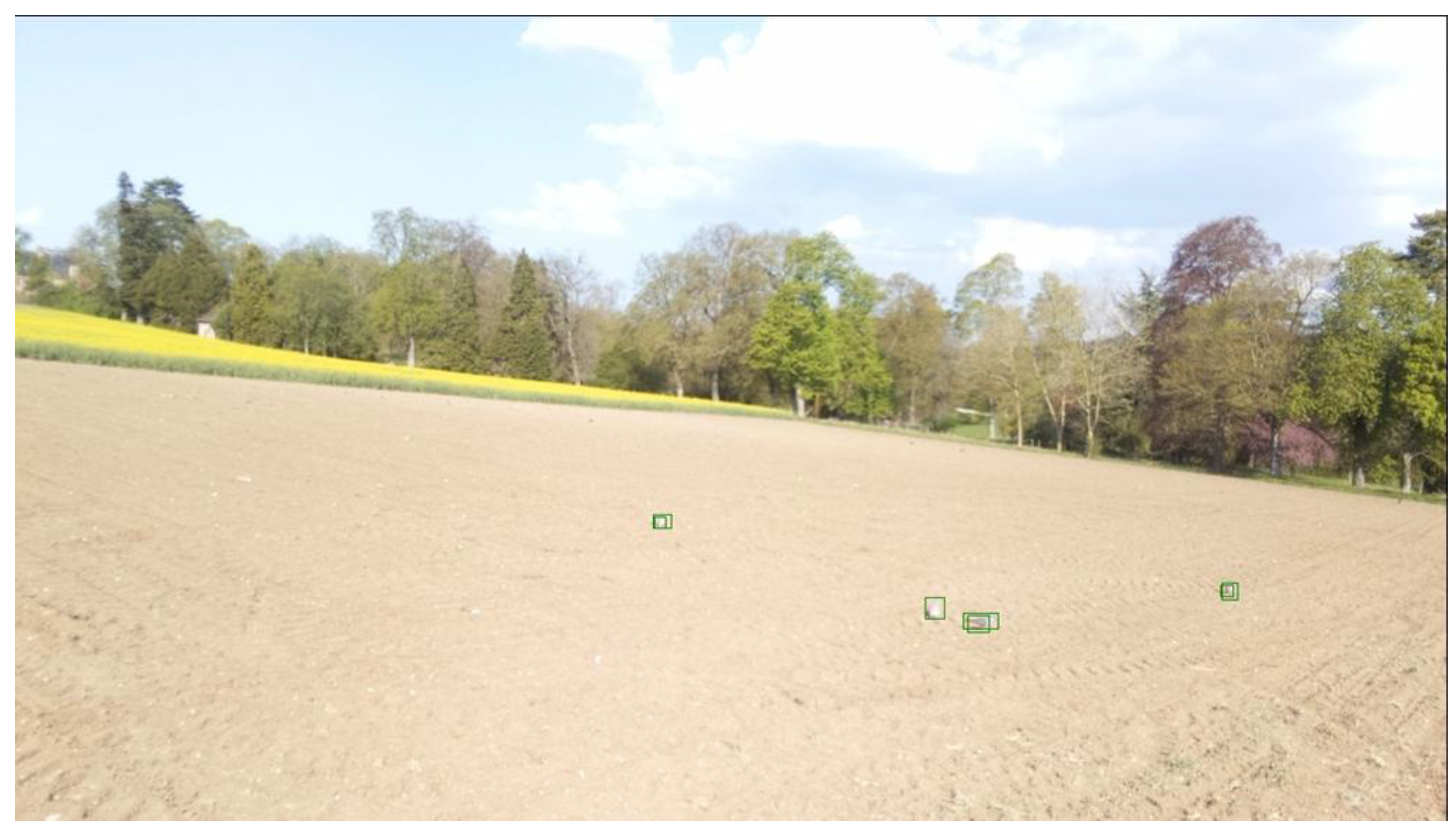
The color of the soil and in general, lighting conditions (at dawn or sunset), and weather make it difficult to detect individuals. In the background it’s very difficult to distinguish other pigeons as they blend in with the ground. To annotate the images, you need to zoom in on each image and annotate everyone carefully. Despite precautions, there are always omissions that must be minimized as much as possible for greater model accuracy.
For the corvids, TP = 12, FN=3+0=3, and FP=3+0= 3
Precision=12 / (12+3) = 0.80 so 80.00%
Recall= 12 / (12+3) = 0.80 so 80.00%
For the pigeons TP= 4, FN= 0+0 = 0 and FP= 0+0= 0
Precision=4 / (4+0) = 1.00 so 100%
Recall= 4 / (4+0) = 1.00 so 100%
Figure 4.
In this image, 12 corvids are detected (green color) ouother presents (red color), i.e., TP=12, and 3 corvids are not detected, i.e., FN=3.
Figure 4.
In this image, 12 corvids are detected (green color) ouother presents (red color), i.e., TP=12, and 3 corvids are not detected, i.e., FN=3.
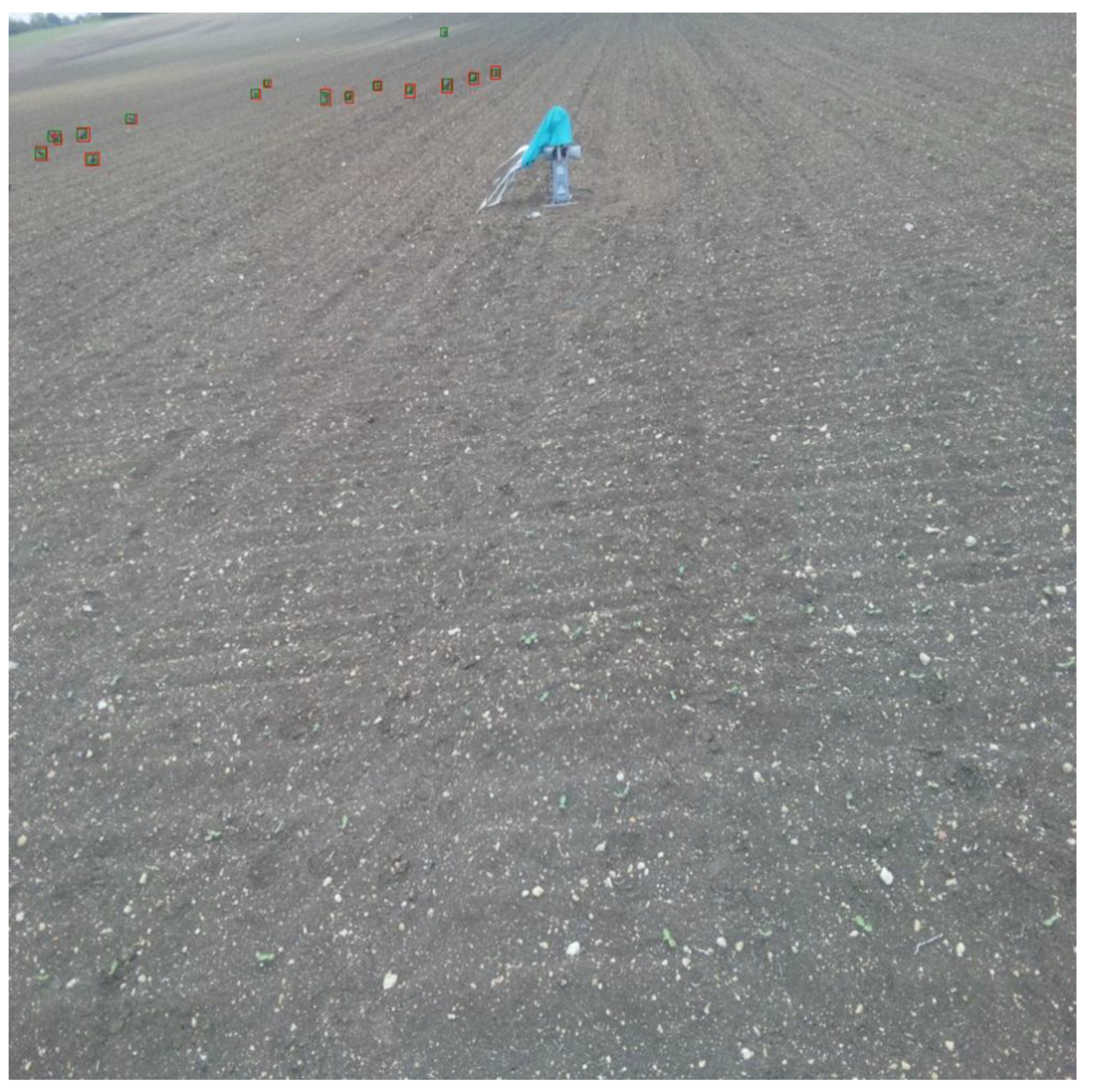
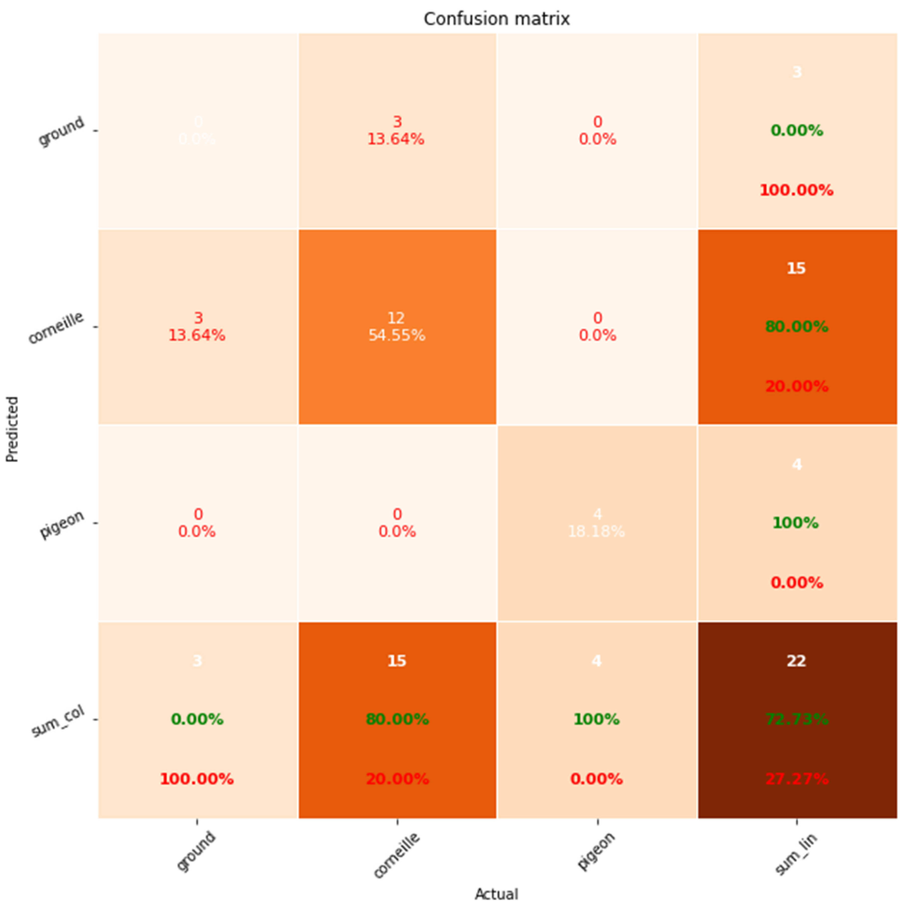
Figure 5.
An educational example of calculating a confusion matrix on a dataset of two images.
4. Model Construction
4.1. Training Phase
After building our BirdyDataset of 3,099 annotated images, we adapted Mask-RCNN to our context.. Out of a hundred or so meta parameters, we focused on just a few: Also, various configurations were tested with the best results obtained with these appropriate hyperparameter values:
Anchor scale: [16,32,64,128,256]
learning rate: 0.0006
IoU in learning phase is set to 0.35
Iou in detection phase is set to 0.5
IMAGE_MAX_DIM: 1024
IMAGE_MIN_DIM: 500
Batch size: 3099
The different stages of the learning phase yielded these results:
Epoch 1/10
3099/3099 [==============================] - 1036s 334ms/step - loss: 0.3905 - val_loss: 2.0688
Epoch 2/10
3099/3099 [==============================] - 992s 320ms/step - loss: 0.3162 - val_loss: 2.5383
Epoch 3/10
3099/3099 [==============================] - 990s 319ms/step - loss: 0.2732 - val_loss: 1.2451
Epoch 4/10
3099/3099 [==============================] - 994s 321ms/step - loss: 0.3108 - val_loss: 3.2857
Epoch 5/10
3099/3099 [==============================] - 994s 321ms/step - loss: 0.2524 - val_loss: 1.7954
Epoch 6/10
3099/3099 [==============================] - 994s 321ms/step - loss: 0.2591 - val_loss: 2.4610
Epoch 7/10
3099/3099 [==============================] - 994s 321ms/step - loss: 0.2440 - val_loss: 2.3251
The learning curve graph shows that epoch 5 has good values for loss (0.2524) and val_loss (1.7954). We therefore chose this epoch as optimal and to avoid overfitting. Calculating the confusion matrix for this learning phase gives us:
Figure 6.
Confusion matrix for the train of 3099 images, learning-rate=0.0006, epoch=5, IoU=0.5.
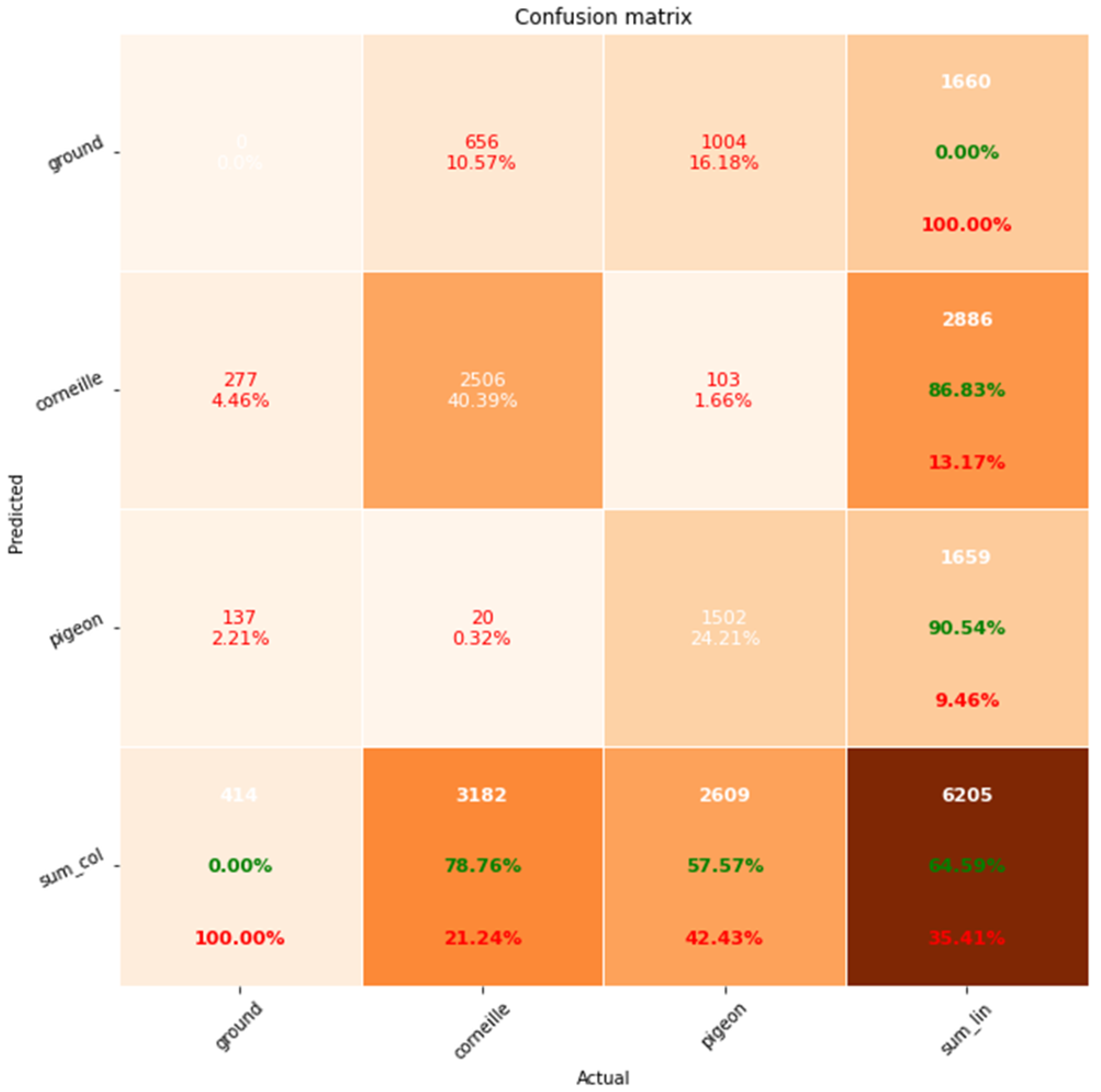
For the corvids, TP = 2506, FN=277+103=380, and FP=20+656= 676
Precision=2506 / (2506+676) = 0.7876 so 78.76%
Recall= 2506 / (2506+380) = 0.8683 so 86.83%
For the pigeons TP=1502, FN= 137+20 = 157 and FP= 1004+103= 1007
Precision=1502 / (1502+1007) = 0.5757 so 57.57%
Recall= 1502 / (1502+157) = 0.9054 so 90.54%
We can see that corvids are better recognized than pigeons. This is because the color of the pigeon often blends in with the ground and therefore becomes less easily detectable. Images are taken from dawn to sunset. Lighting conditions as well as weather (clouds, rain) and ground color are of course very important for bird detection.
4.2. Model Optimization by Eliminating Large Individuals from BirdyDataset
Since the hyperparameters of our model are geared toward detecting small and medium-sized individuals, and since only 1.23% of the individuals in our BirdyDataset are large (Table 2), we removed these individuals to see how the model would perform. Our new BirdyDataset now contains 3,030 images of small and medium-sized individuals. We then built a new learning model based on this new dataset. We found that the accuracy (76.66%) and recall (55.43%) for corvids did not change much, but there was a significant improvement in the accuracy (74.54%) and recall (56.27% for pigeons (Figure 7). So, as a first observation, our model performs better with small and medium-sized objects, which makes perfect sense. Next, we can build a model dedicated to large objects.
The accuracy of both classes is better than in the previous model. Therefore, filtering out large individuals improves the model’s performance, as it is designed for small and medium individuals. We also note that for both classes, recall is lower than precision. Our goal is to trigger an alarm as soon as a certain number of birds are present in the plot. For us, precision is more important than recall. To validate our model, we proceeded in two ways: qualitative validation and quantitative validation
5. Results
5.1. Qualitative Validation
Qualitative validation is based on data collected by farmers during the years 2022, 2023, and 2024. We monitored several plots in different regions of the country, located using their GPS coordinates. For each plot, we recorded 23 columns of metadata such as crop and cropping system, as well as damage caused by corvids and pigeons and its intensity. The intensity of the damage is described by four qualitative values: no attack, weak attack, moderate attack, and strong attack. This metadata is stored in csv format as shown in Figure 8:
In the Python ecosystem, Lambda functions and the Pandas library allow us to query our databases in a simple and concise manner. For example, to find out which plots are most intensely damaged by corvids and pigeons, but before formulating this question, we must first read our metadata by this Pandas function such as:
dataframe = pandas.read(working_dadaset, “metadata.csv”)
And the query to find out which plots have been attacked by both corvids and pigeons can be written as follows:
dataframe[‘newcolumn’]= dataframe.apply(lambda x: (x.corvid_damage==‘yes’) & (x.corvid_damage_intensity==‘strong’) & (x.colombid_damage==‘yes’) & (x.colombid_damage_intensity ==‘yes’), axis=1)
dataframe_both_damage = dataframe[dataframe[“newcolumn”] == True]
The result of the query gives us the identificators of the plots attacked:
dataframe_both_damage
“la_vallee_grand_jean”
If we query the simulated data database, i.e., the results of automatic annotation for the plot “La Vallée Grand Jean” in the year 2023, we can see from the graph in the Figure 9, that there was indeed a severe attack by corvids in April. This confirms the farmer’s observation. More generally, we can find out which plots are moderately attacked or those that were not attacked at all.
Another way to visualize the temporality of birds is to focus on their presence during the day. If we look at the number of individuals according to the time of day, we see that the highest number of individuals is between 10 a.m. and 2 p.m. (Figure 10).
5.2. Quantitative Validation
Over the past 4-5 years, we have acquired more than 15 TB of raw images taken in different plots located in four regions in France. We have annotated several thousand of these images. We compared these manual annotations with the results of automatic annotation to validate our model.
Each automatic annotation line contains 14 columns of data, including the annotated image, the model, the number of corvids and pigeons and their bounding boxes (Figure 11).
For the year 2024, we annotated 2753 new JPG images, i.e., images that were not used in the learning phase. These annotated images, in Json format, were converted to xml format to be used by our processing pipelines. These images contain 547 corvids and 165 pigeons. As a result, many of the images show no individuals other than the plot. This gives us the opportunity to test all the images to see whether they contain individuals.
Therefore, we compared the centers of simulated bounding boxes (in blue) and observed bounding boxes (in red). The points at the top of the graph (Figure 12) are the furthest from the camera and, conversely, the points at the bottom, closest to 0, are the closest to the camera. We note that the observed/predicted points overlap well and that most of these points are at the top of the graph, far from the camera lens.
In addition, we tracked the temporal dynamics of the number of individuals. We counted the number of simulated individuals based on time (day and hour), and the number observed from dawn to sunset (Figure 13). We observe a fairly good overlap between the simulated and observed values, with a slight underestimation by the model.
6. Discussion/Conclusions
Scarecrows are currently undergoing numerous developments, both in terms of repulsive signals (e.g., laser, Goswami et al., 2024) and mobility (e.g., flying drone, e.g., Conor et al., 2020). Adding reactivity to these technical components would enhance the efficiency of the scaring devices as tested with drones by Wang, 2021 Nirmala Devi et al., 2024 Yakubu et al., 2025. In our case of large field monitoring, our work takes place upstream of potential commercial developments. What remains to be resolved is the economic equation for proposing efficient tools adapted to large field and crops with low economic margin per hectare. The most plausible development scheme is a coupling with bird-scaring devices covering 5 ha (maximum range of commercial models), or a network of many cameras. This raises the question of the portability of algorithms on low-power, all-terrain equipment.
To limit the damage caused by birds, we initially acquired more than 15 TB of raw images over a period of 4-5 years. In a second step, we developed a method for automatically detecting these birds. To do this, we improved the Mask-RCNN method by acting on the hyperparameters to detect small individuals. This is in fact the main difficulty and challenge for agronomy and computing. To do this, we built several datasets, from the smallest one with 200 images to the most realistic with 3,099 images. By adjusting the hyperparameters of Mask-RCNN and increasing the number of GPU hours on HPC, we were able to build a model adapted to small individuals. The model performs well with a mAP of 78.76% for corvids and 57.57% for pigeons. Next, our terabytes of images acquired in the field were automatically annotated. A small portion of these images, which were not used in the learning phase and were annotated manually, enabled us to validate our model.
Our next goal is to deploy our model in the field by implementing it on a lightweight device consisting of a card such as the Nvidia Jetson Tx2 coupled with a camera.
On the other hand, it should be noted that there are not many datasets for small individuals. Therefore, Birdydataset is an important contribution to pest management practices and could be used as input in other models for improved accuracy and precision. Overall, this study provides a valuable contribution to the field of pest management in agriculture, demonstrating the effectiveness of deep Learning-based object detection models for detecting pests and their potential for integration with real-time spraying technologies.
Abbreviations
The following abbreviations are used in this manuscript:
| BIAD | Bird identification and detection |
| CNN | Convolutional Neural Network |
| RCNN | Region-based Convolutional Network |
| MS-COCO | MicroSoft Common Objects in Context |
| mAP | mean Average Precision |
| TP | True Positive |
| FP | False Positive |
| FN | False Positive |
References
- Chen, G., Wang, H., Chen, K., Li, Z. , Song, Z., Liu, Y., Chen, W., and Knoll, A., A Survey of the Four Pillars for Small Object Detection: Multiscale Representation, Contextual Information, Super-Resolution, and Region Proposal, 2168-2216, 2020 IEEE. [CrossRef]
- Conor C Egan, Bradley F Blackwell, Esteban Fernández-Juricic, Page E Klug, Testing a key assumption of using drones as frightening devices: Do birds perceive drones as risky?, The Condor: Ornithological Ap-plications, Volume 122, Issue 3, 4 August 2020, duaa014. [CrossRef]
- Félix-Jiménez, A.F.; Sánchez-Lee, V.S.; Acuña-Cid, H.A.; Ibarra-Belmonte, I.; Arredondo-Morales, E.; Ahumada-Tello, E. Integration of YOLOv8 Small and MobileNet V3 Large for Efficient Bird Detection and Classification on Mobile Devices. AI 2025, 6, 57. [CrossRef]
- Fu, H., Wang, C., Benani, N. et al. Bird detection and overall bird situational awareness at airports. Orni-thol. Res. 32, 280–295 (2024). [CrossRef]
- Gilsdorf, J.M., Hygnstrom, S.E. & VerCauteren, K.C. Use of Frightening Devices in Wildlife Damage Management. Integrated Pest Management Reviews 7, 29–45 (2002). [CrossRef]
- Girshick, R., Fast R-CNN, Microsoft Research, 2015. https://arxiv.org/abs/1504.08083.
- Goswami, S., Raghuraman, M., Das, K.K., Gadekar, M., 2024. Laser Scarecrows in Agriculture: An innova-tive solution for bird pests. Biotica Research Today 6(4), 156-157. [CrossRef]
- Guo, Z.; He, Z.; Lyu, L.; Mao, A.; Huang, E.; Liu, K. Automatic Detection of Feral Pigeons in Urban Envi-ronments Using Deep Learning. Animals 2024, 14, 159. [CrossRef]
- He, K., Georgia, G. Gkioxari, P. Dollar, Girshick, R., Facebook AI Research (FAIR), Mask R-CNN, Cornell University, 2018. https://arxiv.org/abs/1703.06870.
- Kisantal, M., Wojna, Z., Murawski, J., Naruniec, J., Cho,K., Augmentation for small object detection, Computer Vision and Pattern Recognition (cs.CV), Feb 2019. https://arxiv.org/abs/1902.07296.
- Lin, T. Y., Maire M, Belongie SJ, Bourdev LD, Girshick RB, Hays J, et al. Microsoft COCO: Common Objects in Context, Computer Vision and Pattern Recognition, 2014, arXiv:1405.0312 [cs.CV].
- Lou, H.; Duan, X.; Guo, J.; Liu, H.; Gu, J.; Bi, L.; Chen, H. DC-YOLOv8: Small-Size Object Detection Algorithm Based on Camera Sensor. Electronics 2023, 12, 2323. [CrossRef]
- Nirmala Devi, L., Subba Reddy, K.V., Nageswar Rao, A. (2025). A Novel Autonomous Bird Deterrent Sys-tem for Crop Protection Using Drones. In: Saini, M.K., Goel, N., Miguez, M., Singh, D. (eds) Agricultural-Centric Computation. ICA 2024. Communications in Computer and Information Science, vol 2207. Springer, Cham. [CrossRef]
- Ramos, L., Casas, E., Bendek, E., Romero, C., Rivas-Echeverría, F., Hyperparameter optimization of YOLOv8 for smoke and wildfire detection: Implications for agricultural and environmental safety, Artificial Intelligence in Agriculture, Volume 12, 2024, Pages 109-126, ISSN 2589-7217,. [CrossRef]
- Redmon, J., S. Divvala, R. Girshick, A.Farhadi, You Only Look Once: Unified, Real-Time Object Detection, Computer Vision and Pattern Recognition, 2015, arXiv:1506.02640 [cs.CV].
- Ren, S., He, K., Girshick, R., Sun, J., Faster R-CNN: Towards Real-Time Object Detection with Region Proposal Networks, 2016. https://arxiv.org/abs/1506.01497.
- Oviedo, M. R., Mendonca, F. A., Cabrera, J., McNall, C. A., Ayres, R., Barbosa, R. L., & Gallis, R. (2024). Automatic detection of birds in images acquired with remotely piloted aircraft for managing wildlife strikes to civil aircraft. International Journal of Aviation, Aeronautics, and Aerospace, 11(4). [CrossRef]
- Sausse, C., Baux, A., Bertrand, M., Bonnaud, E., Canavelli, S., Destrez, A., ... & Zuil, S. (2021a). Contem-porary challenges and opportunities for the management of bird damage at field crop establishment. Crop Protection, 148, 105736.
- Sausse, C., Chevalot, A., & Lévy, M. (2021b). Hungry birds are a major threat for sunflower seedlings in France. Crop Protection, 148, 105712.
- Schiano F.,Natter, D., Zambrano D. and Floreano, D. Autonomous Detection and Deterrence of Pigeons on Buildings by Drones, in IEEE Access, vol. 10, pp. 1745-1755, 2022. [CrossRef]
- Shapetko, E. V., Belozerskikh, V. V., & Siokhin, V. D. (2024). Implementation of artificial intellect for bird pest species detection and monitoring. Acta Biologica Sibirica, 10, 1033–1046. [CrossRef]
- Sohbi, Y.,Teulé, J.M., Morisseau, A., Serrée, L. Barbu, C., Gardarin, A., A dataset of ground-dwelling nocturnal fauna for object detection and classification, Data in Brief, Volume 54, June 2024, 110537. [CrossRef]
- Yakubu, I., Audu, M. M., & Zayyanu, Y. (2025). UNMANNED AERIAL VEHICLE (UAV)-BASED COM-PUTER VISION MODEL FOR REAL-TIME BIRDS DETECTION IN RICE FARM. Open Journal of Phys-ical Science (ISSN: 2734-2123), 6(1), 1-13. [CrossRef]
- Wu, Q.; Feng, D.; Cao, C.; Zeng, X.; Feng, Z.; Wu, J.; Huang, Z. Improved Mask R-CNN for Aircraft De-tection in Remote Sensing Images. Sensors 2021, 21, 2618. [CrossRef]
- Wang, X.; Wang, A.; Yi, J.; Song, Y.; Chehri, A. Small Object Detection Based on Deep Learning for Re-mote Sensing: A Comprehensive Review. Remote Sens. 2023, 15, 3265. [CrossRef]
- Zhou, C., Lee, W.S., Liburd, O.E, Aygun, I., Zhou, X., Pourreza, A., Schueller, J.K., Ampatzidis, Y., Detecting two-spotted spider mites and predatory mites in strawberry using deep learning, Smart Agricultural Technology,Volume 4, 2023, 100229, ISSN 2772-3755,. [CrossRef]
- pour la méthode DL car petits individus, à voir cette revue.
- Zhu, J., Ma, C., Rong, J., & Cao, Y. (2024). Bird and UAVs recognition detection and tracking based on improved YOLOv9-DeepSORT. IEEE Access.
- Zhu, H.; Wang, Y.; Fan, J. IA-Mask R-CNN: Improved Anchor Design Mask R-CNN for Surface Defect Detection of Automotive Engine Parts. Appl. Sci. 2022, 12, 6633. [CrossRef]
| 1 | In fact, in practice the max surface detectable is 81 pixels. |
Figure 1.
An example of image augmentation by mirror symmetry. The original image is on the left and its mirror-symmetrical on the right.
Figure 1.
An example of image augmentation by mirror symmetry. The original image is on the left and its mirror-symmetrical on the right.
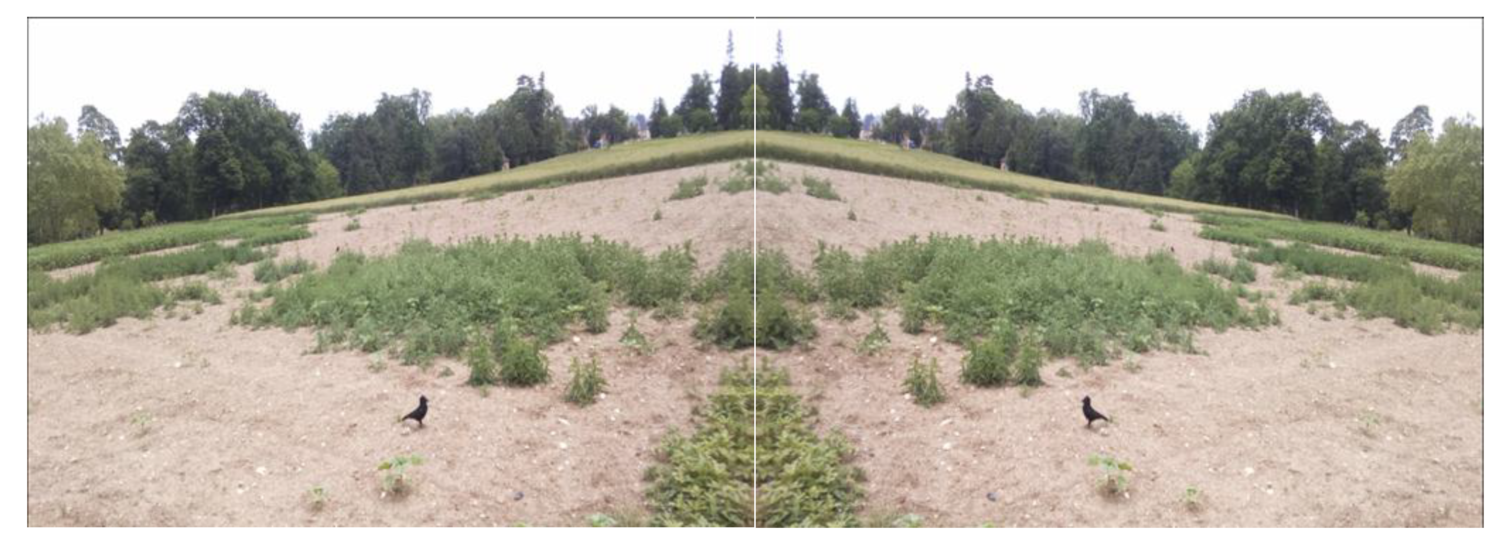
Figure 2.
caption.
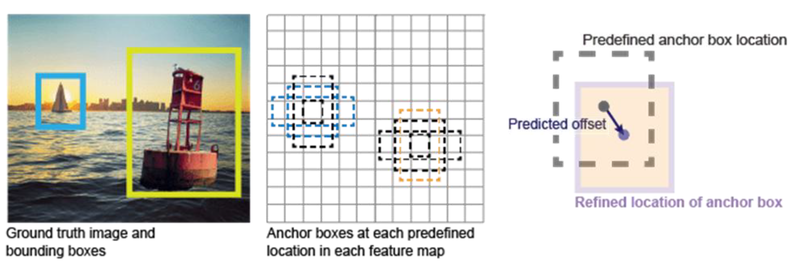
Figure 7.
Confusion matrix of the new Birdydataset (3030 images without large individuals), learning-rate=0.0006, epoch=5, IoU=0.5.
Figure 7.
Confusion matrix of the new Birdydataset (3030 images without large individuals), learning-rate=0.0006, epoch=5, IoU=0.5.
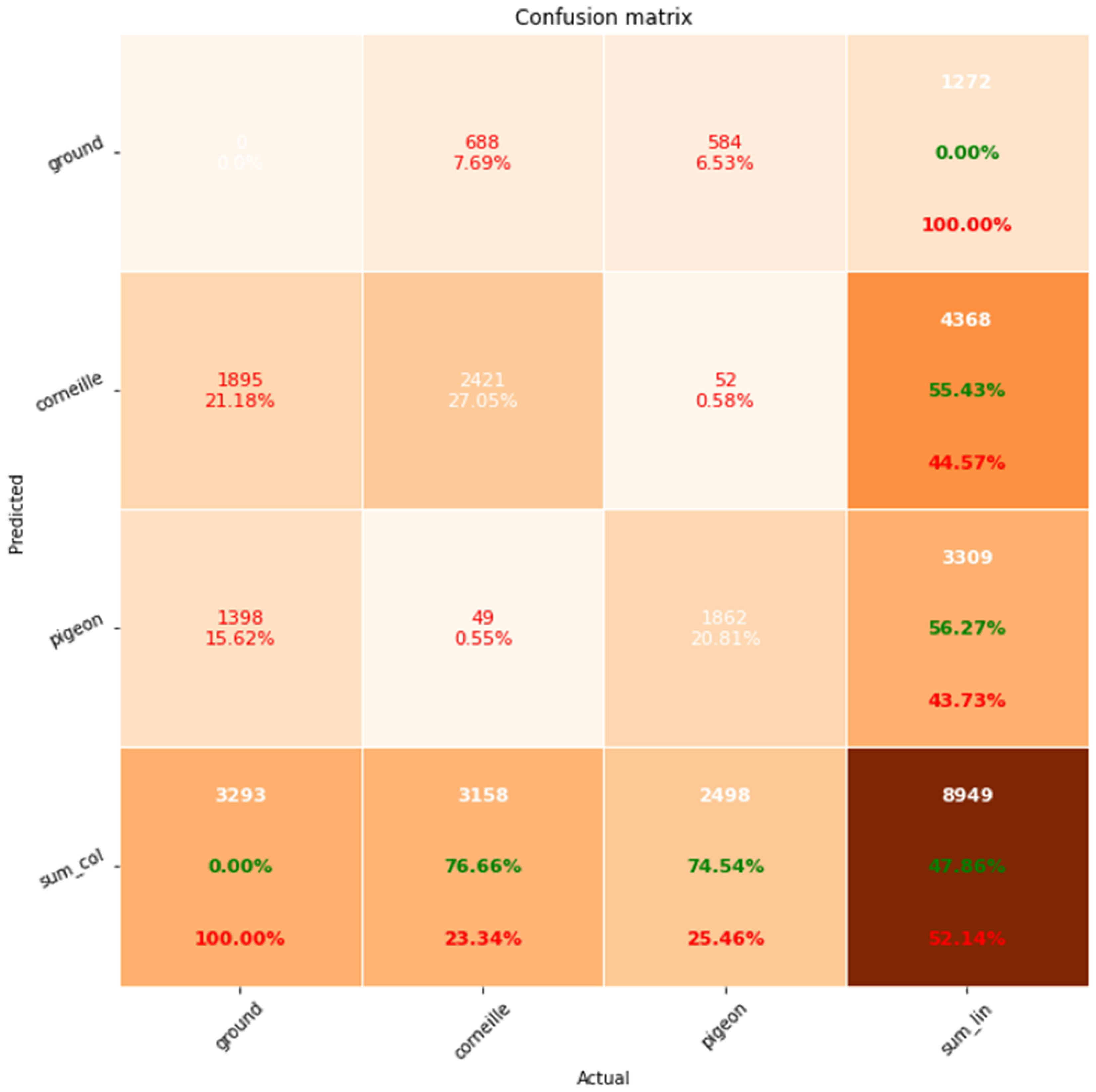
Figure 8.
Meta data on plots, image acquisition, and bird damage for the year 2023.
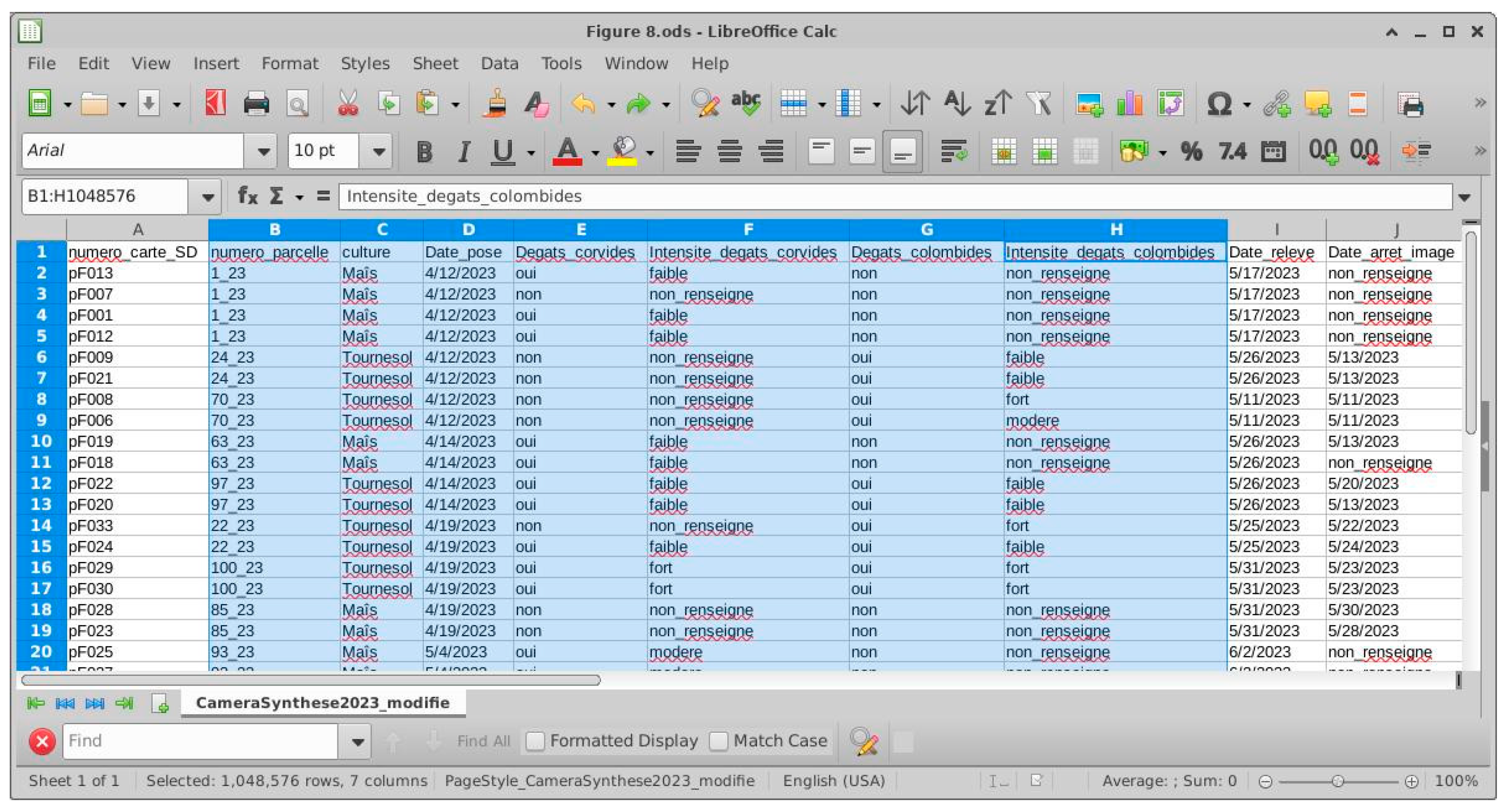
Figure 9.
Results of automatic annotation for the year 2023, with the date on the x-axis and the number of individuals on the y-axis. Significant presence of corvids in April.
Figure 9.
Results of automatic annotation for the year 2023, with the date on the x-axis and the number of individuals on the y-axis. Significant presence of corvids in April.
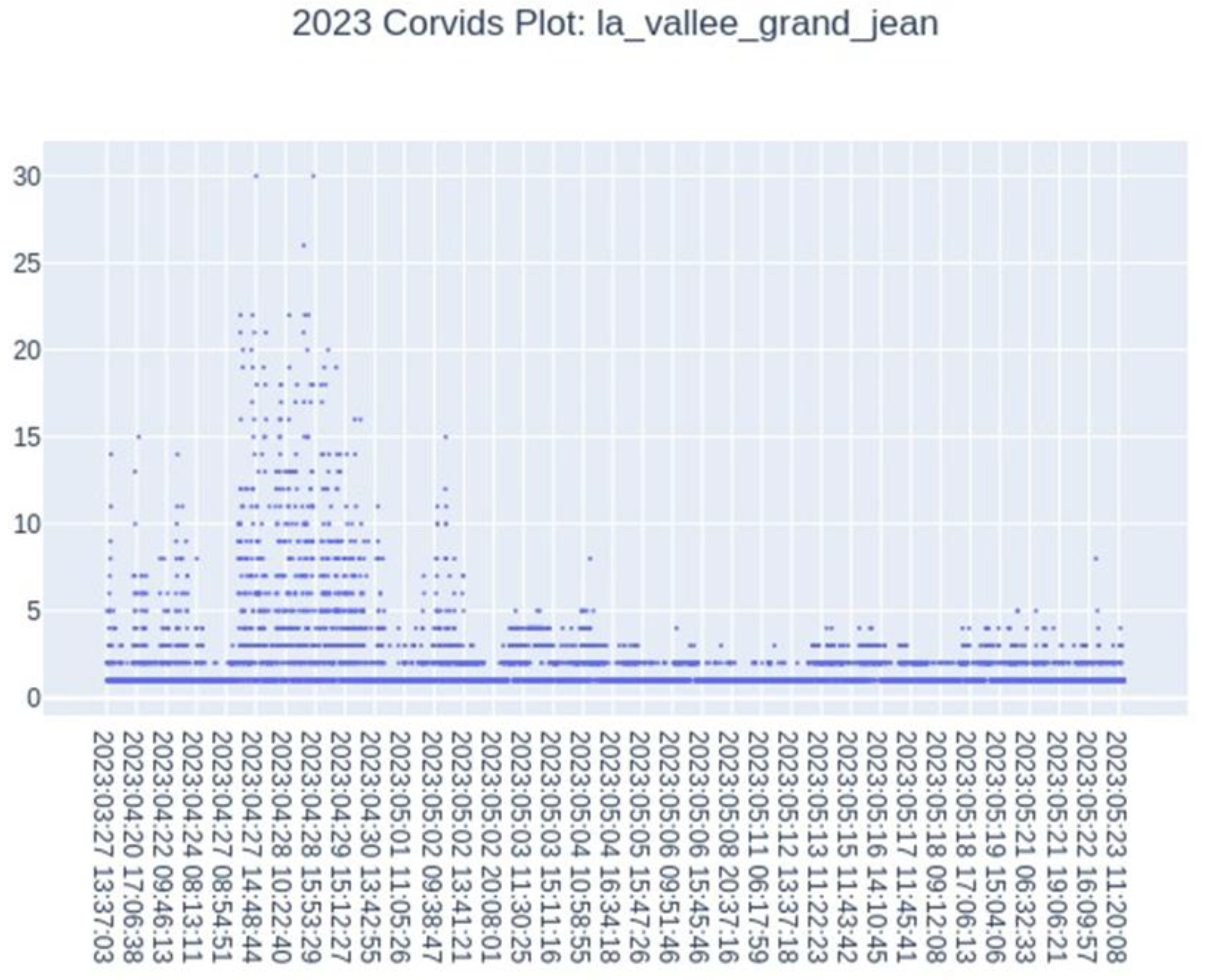
Figure 10.
Results of automatic annotation for the year 2023, on the x-axis, the time from dawn to sunset; on the y-axis, the number of individuals. Significant presence of birds between 10 a.m. and 2 p.m.
Figure 10.
Results of automatic annotation for the year 2023, on the x-axis, the time from dawn to sunset; on the y-axis, the number of individuals. Significant presence of birds between 10 a.m. and 2 p.m.
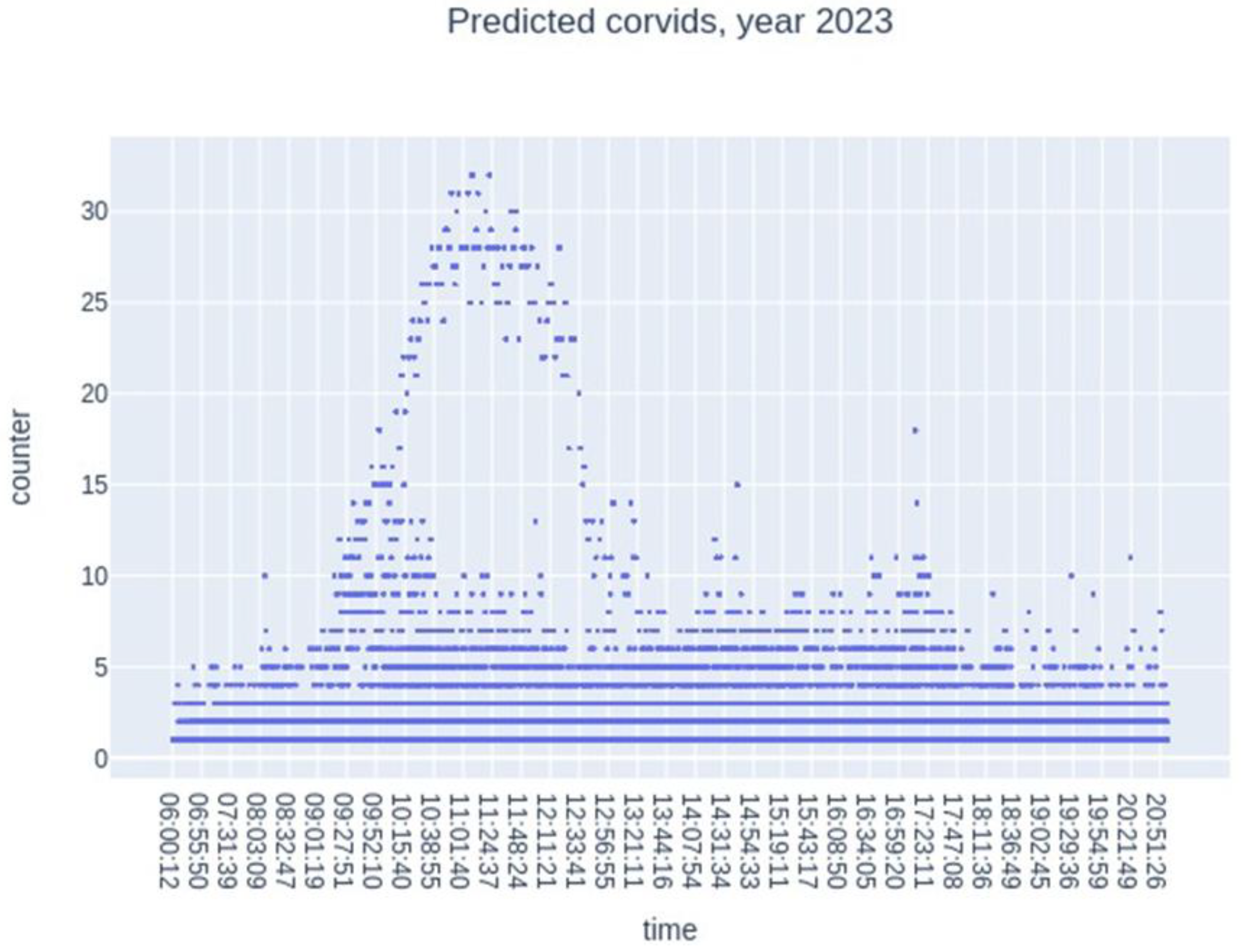
Figure 11.
Automatic annotation metadata:14 columns of metadata including information on annotated images, the number of corvids and pigeons present, and the coordinates of bounding boxes.
Figure 11.
Automatic annotation metadata:14 columns of metadata including information on annotated images, the number of corvids and pigeons present, and the coordinates of bounding boxes.
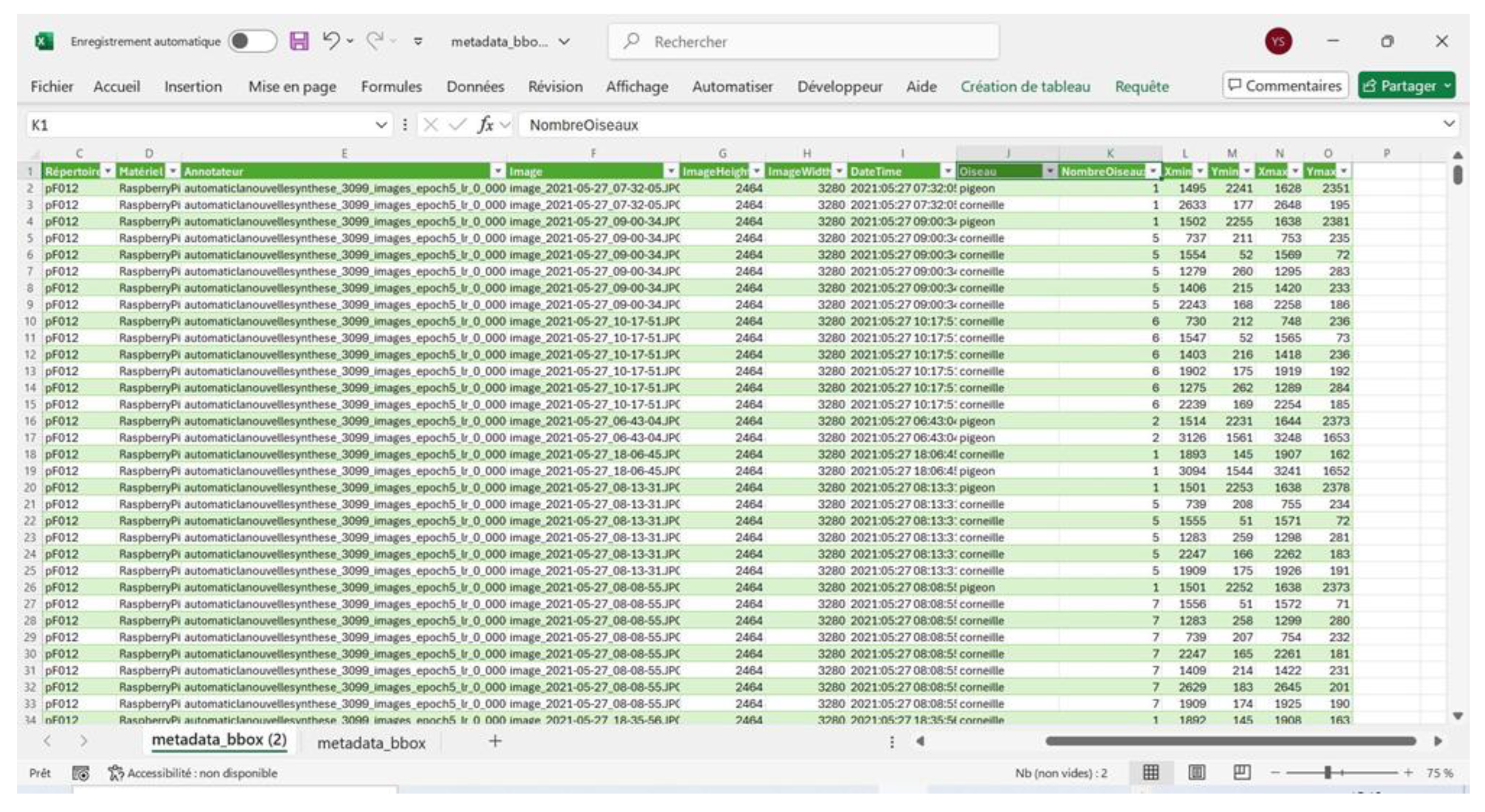
Figure 12.
Year 2024, comparison of manually (red color) and automatically (blue color) annotated bounding box centers.
Figure 12.
Year 2024, comparison of manually (red color) and automatically (blue color) annotated bounding box centers.
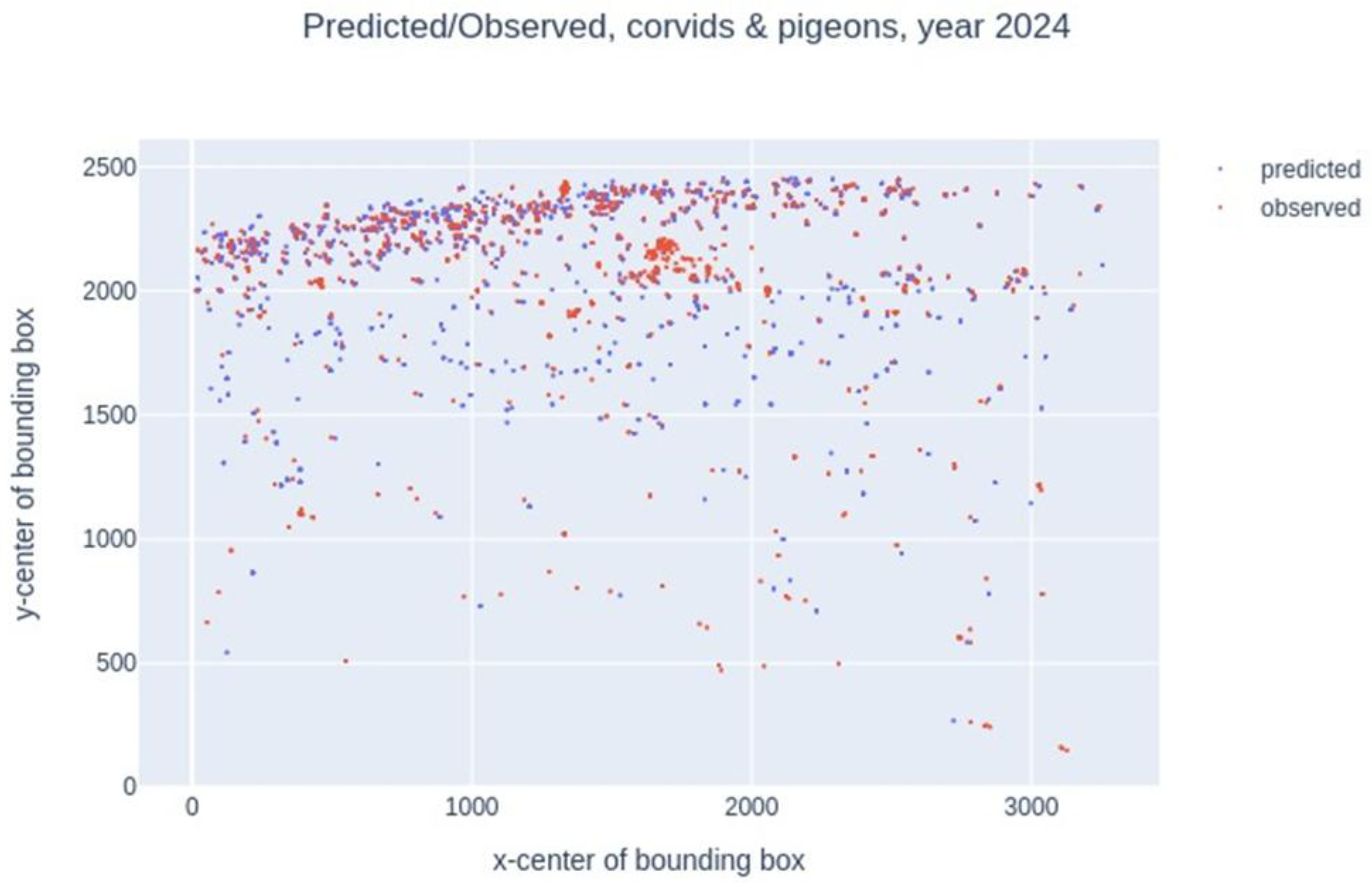
Figure 13.
Year 2024, number of simulated individuals (in blue) and observed individuals (in red) over time. The data overlaps quite well.
Figure 13.
Year 2024, number of simulated individuals (in blue) and observed individuals (in red) over time. The data overlaps quite well.
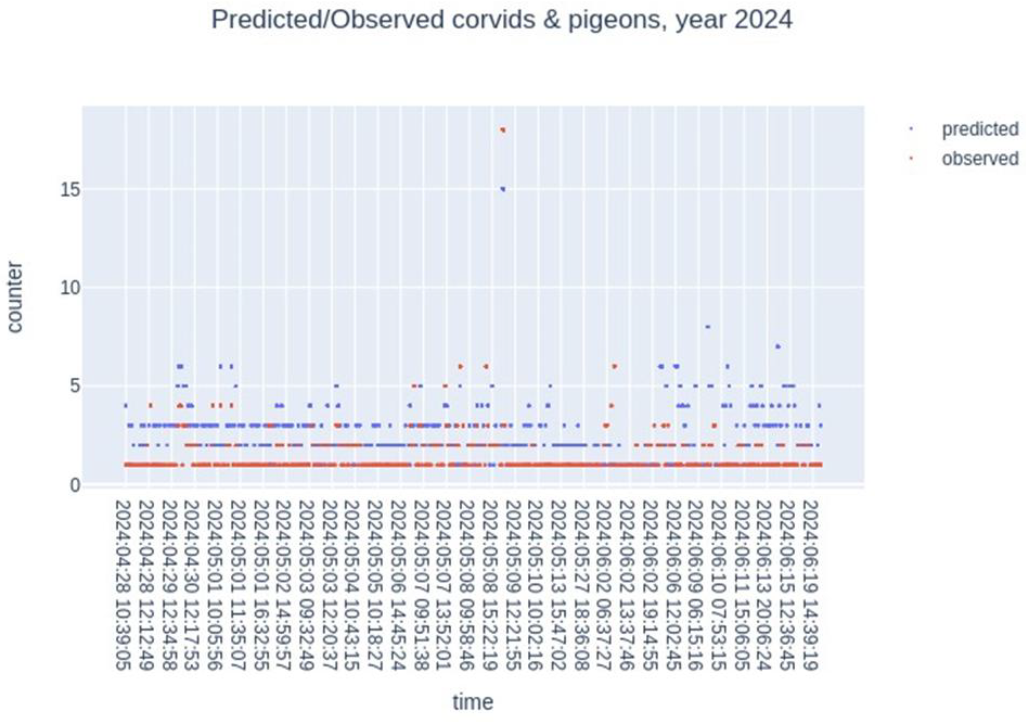

Table 1.
The definitions in pixel size of the small, medium and large objects in MS COCO. 1
Table 1.
The definitions in pixel size of the small, medium and large objects in MS COCO. 1
| Min rectangle area | Max rectangle area | |
|---|---|---|
| Small object | 0x0 | 32x32 |
| Medium object | 32x32 | 96x96 |
| Large object | 96x96 |
Table 2.
The distribution of small, medium and large objects in BirdyDataset.
| Number of images | Number of individuals | Number of corvids & pigeons |
Percentage | |
|---|---|---|---|---|
| Small object | 2645 | 5007 | 2858+2149 | 86.79% |
| Medium object | 582 | 691 | 295+396 | 11.98% |
| Large object | 69 | 71 | 20+51 | 1.23% |
| Total | 3290 | 5769 | 5769 | 100% |
Disclaimer/Publisher’s Note: The statements, opinions and data contained in all publications are solely those of the individual author(s) and contributor(s) and not of MDPI and/or the editor(s). MDPI and/or the editor(s) disclaim responsibility for any injury to people or property resulting from any ideas, methods, instructions or products referred to in the content. |
© 2025 by the authors. Licensee MDPI, Basel, Switzerland. This article is an open access article distributed under the terms and conditions of the Creative Commons Attribution (CC BY) license (http://creativecommons.org/licenses/by/4.0/).
Copyright: This open access article is published under a Creative Commons CC BY 4.0 license, which permit the free download, distribution, and reuse, provided that the author and preprint are cited in any reuse.


