Bias Detection in Plant Species Classification: A Grad-CAM Analysis Reveals Light-Color Dependencies Across CNN Architectures

1. Introduction

Artificial Intelligence has undergone rapid evolution in recent years, transforming from theoretical concepts into practical applications with significant real-world impacts across healthcare, education, and security sectors [10]. This transformation has been driven by intelligent machines with adaptive capabilities, reasoning, and learning abilities, fueled by the abundance of data that propels machine learning advancement into diverse industries. Notably, AI has demonstrated unprecedented results in solving complex numerical and computational problems, shaping the future of human society [24].

Autonomous AI-powered systems, now prevalent in fields like defense, law, and medicine, raise critical needs to understand their decision-making processes [6]. The field faces a fundamental dichotomy between earlier “white-box” models, which provide explainable results but lack state-of-the-art performance [19], and recent “black-box” models like deep learning, which achieve high performance but are challenging to interpret [3,11,17].

The adoption of black box machine learning models in crucial sectors such as healthcare and security raises moral concerns about fairness, transparency, and the reliability of uninterpretable decisions [12]. Stakeholders demand understanding and justification for decisions made by these complex models [8]. Skepticism surrounding the use of uninterpretable techniques, coupled with rising emphasis on ethical AI, has led to the emergence of Explainable Artificial Intelligence (XAI) [26].

XAI has become one of the recent focuses in the scientific community, shifting attention from solely predictive algorithms to understanding and interpreting AI system behavior. The goal is to create more reliable and explainable models while maintaining high-level learning performance, ultimately bridging the trust gap with stakeholders [14]. Plant species classification presents an ideal domain for XAI exploration, acknowledging the challenges posed by vast variations in plant characteristics [22]. Despite global biodiversity decline [16], accurate knowledge of plant identity and distribution remains crucial for future biodiversity endeavors [9].

This project aims to explore the explainability of a plant species classifier, with a focus on applying Explainable Artificial Intelligence to enhance the transparency of deep learning models, specifically Convolutional Neural Networks (CNNs). We employed Grad-CAM, a technique for generating visual explanations, to gain deeper understanding of these models’ decision-making processes. The significance of this project lies in its ability to bridge the gap between plant classification with deep learning and explainable artificial intelligence on plant species.

2. Literature Review

2.1. Background on Explainability and Interpretability

“Explainability” and “interpretability” are often used interchangeably, yet they differ in concepts and ideologies [4,12]. While attempts have been made to clarify these terms, there is no mathematical evidence supporting their definitions. Interpretability, in the context of AI and machine learning, denotes a model’s characteristics making sense to a human observer, emphasizing intuitive understanding [4]. In contrast, explainability in AI focuses on the internal logic and procedures within a model or machine learning system [5]. Explainable Artificial Intelligence (XAI) centers on decision understandability for end-users, with challenges in quantifying interpretability gain [8]. XAI is defined as an approach providing details to make a model’s functionality easy to understand [2].

In plant classification, a crucial task in plant taxonomy, CNN models have proven effective. However, there is a need to understand how these models make their choices. Wäldchen et al. [23] used a CNN model to investigate explanatory factors for plant classification due to its precision in achieving results.

2.2. Explainable AI (XAI)

AI systems can be hard to understand and operate like a mystery box, popularly known as the `black box.’ Adadi and Berrada [1] pointed out how tough it is to trust these systems and introduced Explainable AI (XAI), which helps us see inside the mystery box and understand how AI works. They also identified problems with XAI, including lack of clear evaluation methods and trade-offs between understandability and prediction accuracy.

Guidotti et al. [7] provided additional details, discussing challenges in explaining black box models. In their work, they mentioned the need to specify what kind of explanations are wanted, either for a part (local) or for the whole system (global). They also discussed different types of black box models, acknowledging diversity in models like neural networks and support vector machines. Explaining these models is complicated, considering the massive data involved and intricate relationships.

Murdoch et al. [15] emphasized the importance of making AI systems understandable, helping find errors and biases. However, they recognized challenges in finding balance between understanding and making accurate predictions. They noted that measuring how understandable AI is can be difficult and that there’s no ultimate solution for making AI systems understandable—it depends on the specific application.

Overall, these studies show that AI systems are difficult to understand and there’s no one perfect solution, hence the need to find appropriate ways to understand AI operations so that we can trust and use AI confidently in our daily lives.

2.3. Plant Classification Using Deep Learning

In 2018, Xiao et al. [25] proposed a novel approach to plant species identification in real-world images using deep convolutional neural networks (CNNs) and visual attention. Their framework utilizes visual attention to crop images to focus on plants, followed by CNNs to classify species. They evaluated their approach on two datasets and found that it outperforms other methods.

Liu et al. [13] investigated plant species classification using hyperspectral imaging and deep learning. They addressed limitations of traditional RGB imaging for plant species classification and introduced a lightweight convolutional neural network (CNN) model for hyperspectral image classification. The CNN model, called LtCNN, achieved a kappa coefficient of 0.95 for plant species classification, outperforming other CNN models. The authors found that using green-edge (591 nm), red-edge (682 nm), and near-infrared (762 nm) bands from hyperspectral images was most effective for classifying plant species.

Generally, there is no direct work done on the explainability of plant species classification. In this project, we used the Grad-CAM technique on visual explanations for decisions made by CNNs to explain what occurs within the models. It is important to note that Grad-CAM operation is based on gradients of a specific target to result in a coarse localization map of highlighted significant portions/regions of an image [20]. This raises the question: is Grad-CAM able to contribute to visual explanations for CNN decisions in plant classification, and how does it aid in identifying dataset biases?

3. Materials and Methods

3.1. Data Description

Two datasets of different plant species were downloaded from Kaggle [18,21]. The first contains 100 different plant species, referred to as the 100 plant species dataset, and the second contains 30 plant species.

The 100 species plant dataset contains 39,354 images of plant species and was split into 31,438 train and 7,916 test directories. It originally had both image and XML files which were separated for image classification. The average height and width of images were 596.83 and 578.35 pixels respectively for the train folder and 596.64 and 579.09 pixels for the test folder.

The 30 species plant dataset contains 30,000 plant images, with 1,000 images per class and a diverse collection of 30 plant classes and 7 plant types, including crops, fruit, industrial, medicinal, nuts, tubers, and vegetable plants. These images were split into 24,000 train, 3,000 test, and 3,000 validation directories. The train folder has an average height and width of 378.19 and 482.24 pixels, while the test has 366.77 and 475.18 pixels, and the validation folder has 372.76 and 478.63 pixels.

3.2. Dataset Visualization

Figure 1. Size distribution histograms showing height and width distributions for train, test, and validation images. Top two panels show the 100 species dataset, bottom panel shows the 30 species dataset.

Figure 1. Size distribution histograms showing height and width distributions for train, test, and validation images. Top two panels show the 100 species dataset, bottom panel shows the 30 species dataset.

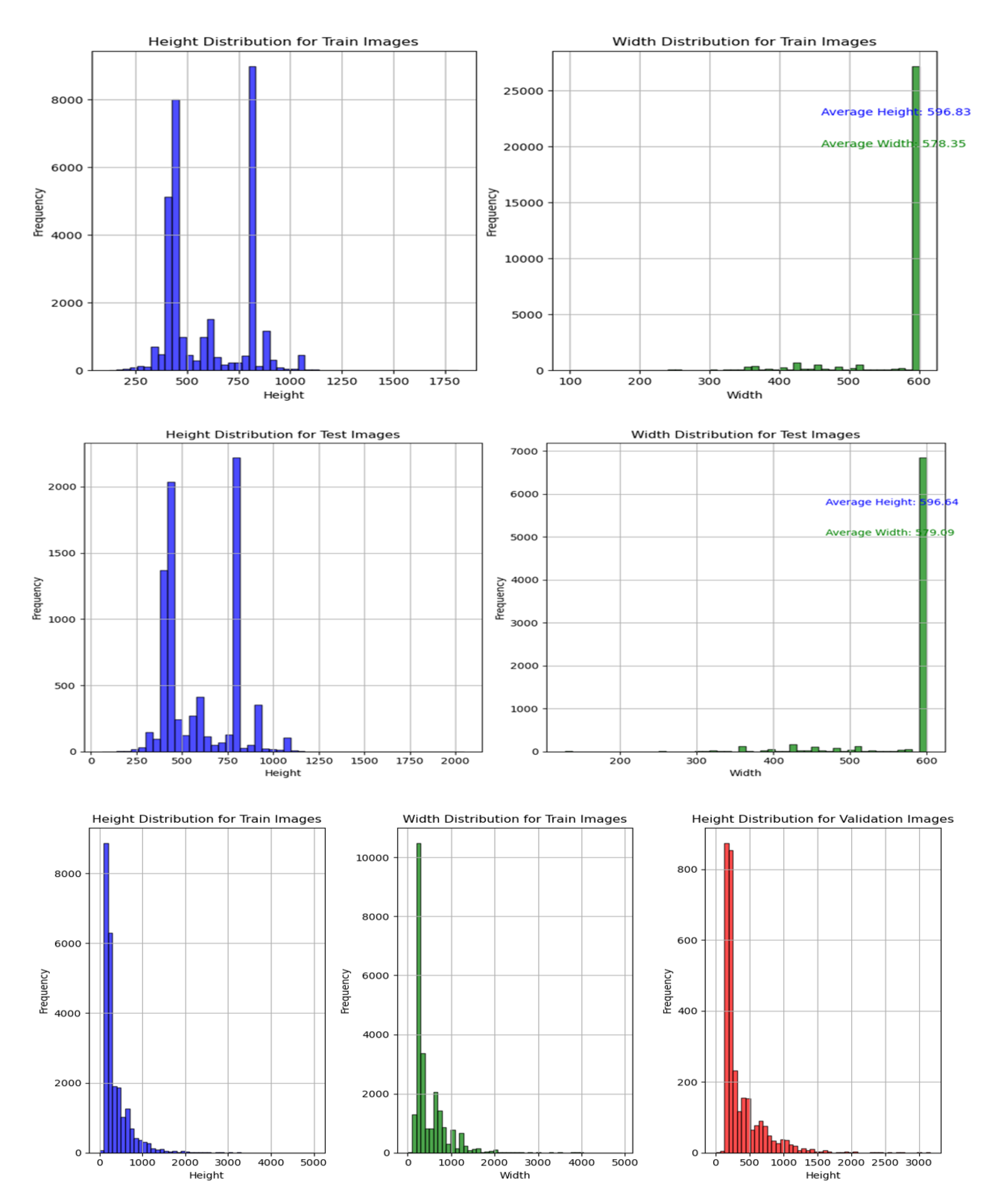
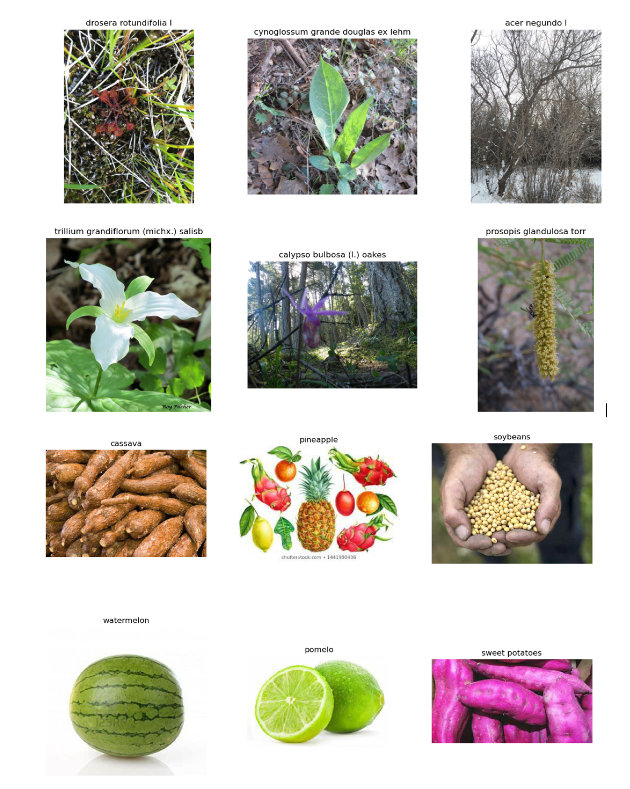
Figure 2. Representative sample images from both datasets. Top two rows display examples from the 100 species dataset showing various plant types at different growth stages. Bottom two rows show samples from the 30 species dataset including crops, fruits, and other plant categories.

Figure 2. Representative sample images from both datasets. Top two rows display examples from the 100 species dataset showing various plant types at different growth stages. Bottom two rows show samples from the 30 species dataset including crops, fruits, and other plant categories.

3.3. Image Preprocessing

For consistency, both datasets were uniformly resized to dimensions of 224×224 pixels. Analysis was first conducted on original-sized images and later on resized images.

3.4. Model Construction and Architecture

For analysis of all plant species, five different models were employed, consisting of two custom-developed Convolutional Neural Network (CNN) models and three pre-trained models.

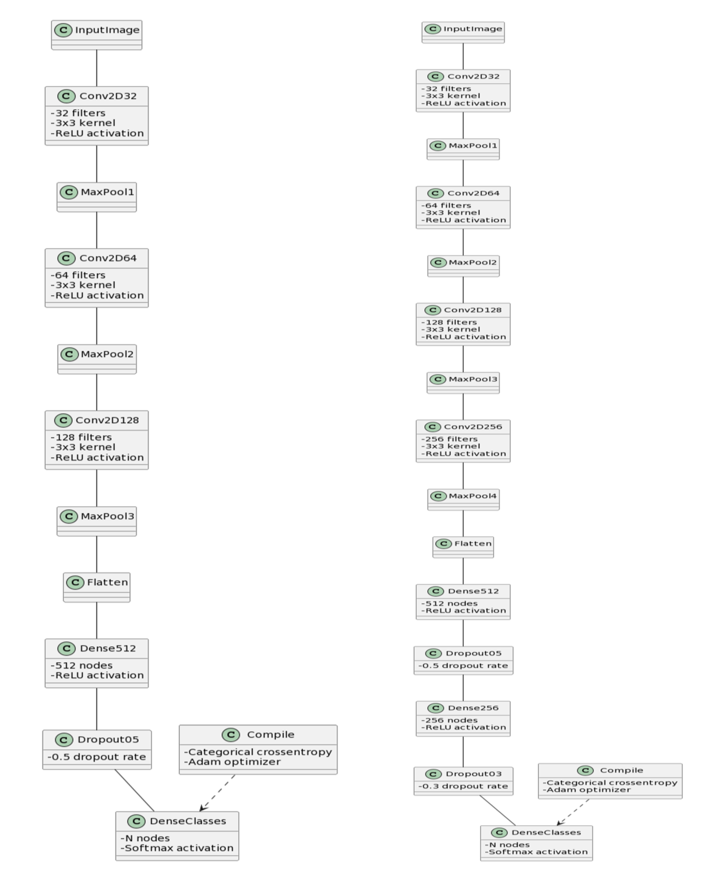
Baseline CNN Model: The Baseline CNN model employed a straightforward architecture, consisting of three convolutional layers, max-pooling layers for down-sampling, and a dense layer for classification. To prevent overfitting, dropout with a rate of 0.5 was incorporated. The model was compiled using the Adam optimizer with a learning rate of 0.0001, utilizing categorical crossentropy loss and accuracy as the evaluation metric. During training, data augmentation techniques were applied to enhance the model’s generalization. The training process was logged over multiple epochs, followed by evaluation on a distinct test dataset.

Improved CNN Model: The Improved CNN model extended the Baseline CNN architecture by introducing an additional convolutional layer and a dropout layer. This augmentation aimed to enhance feature extraction capabilities. Like the Baseline CNN, the model was compiled, trained, and evaluated using the same configuration on a separate test dataset, providing insights into its improved performance.

3.5. Model Architectures

Figure 3. Architecture diagrams of the custom CNN models. (a) Baseline CNN showing three convolutional layers with max-pooling and dense classification layer. (b) Improved CNN with additional convolutional and dropout layers for enhanced feature extraction.

Figure 3. Architecture diagrams of the custom CNN models. (a) Baseline CNN showing three convolutional layers with max-pooling and dense classification layer. (b) Improved CNN with additional convolutional and dropout layers for enhanced feature extraction.

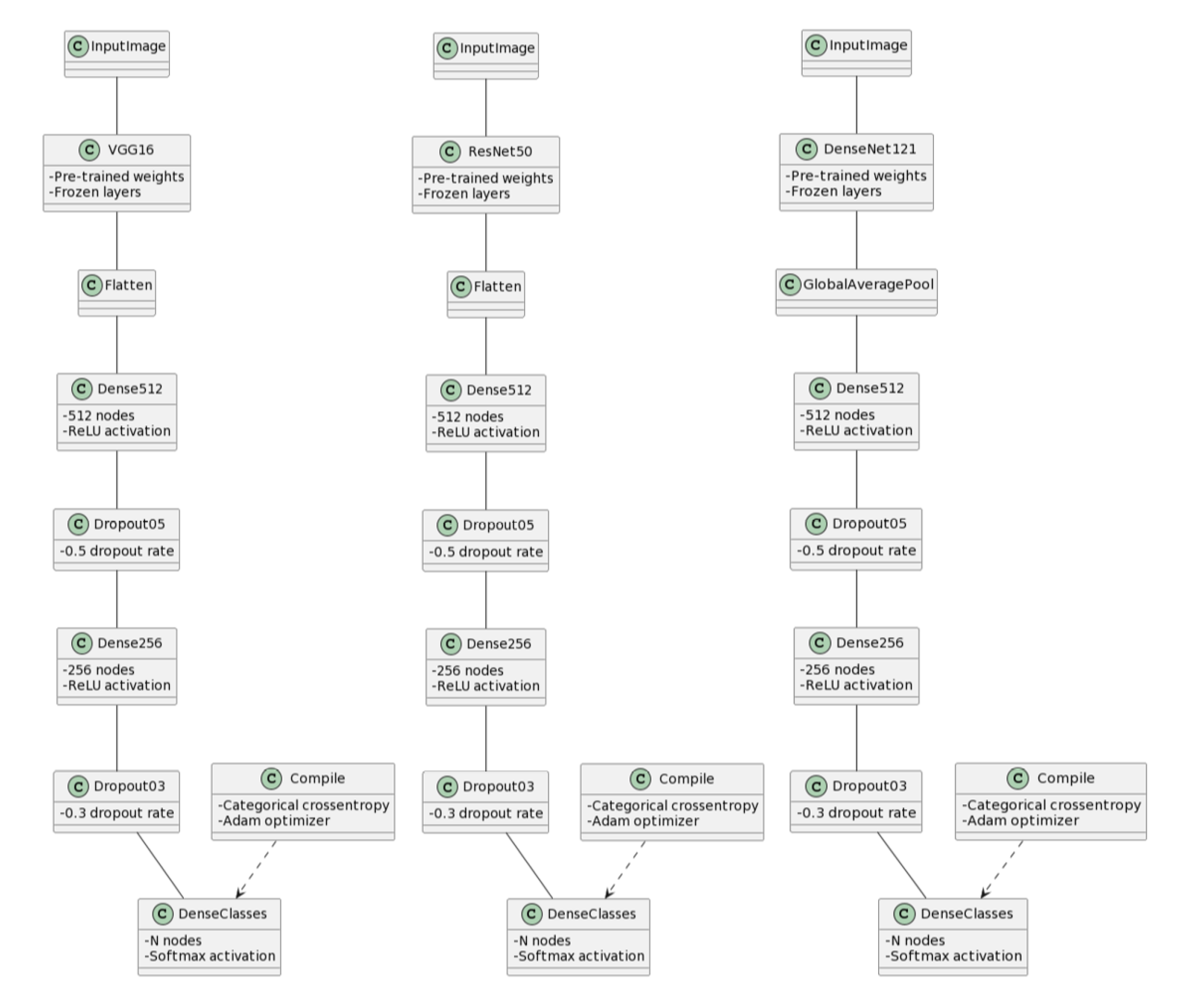
VGG16-Based Transfer Learning Model: The third model utilized transfer learning with the VGG16 architecture. The convolutional base of the pre-trained VGG16 model was employed, and custom fully connected layers were added for classification. To retain learned features, the layers of the pre-trained model were frozen. The model was compiled with the Adam optimizer, featuring a learning rate of 0.0001, and used categorical crossentropy loss and accuracy as evaluation metrics. Data augmentation during training contributed to the model’s robustness, and performance was tracked over epochs before evaluation on an independent test dataset.

ResNet50-Based Transfer Learning Model: Employing a similar transfer learning approach, the fourth model utilized the pre-trained ResNet50 model. Custom fully connected layers were added to adapt the model for the specific classification task. Like the VGG16 model, the layers of the pre-trained ResNet50 model were frozen to retain learned features. The model was compiled, trained, and evaluated using the same configurations as the VGG16 model, providing comparative analysis of the performance of these two architectures.

DenseNet121-Based Transfer Learning Model: The fifth model leveraged transfer learning with the DenseNet121 architecture. Dense blocks and transition layers from the pre-trained DenseNet121 model were utilized, and custom classification layers were added. The layers of the pre-trained model were frozen to preserve learned features. The model’s pipeline and training process were the same as VGG16.

Figure 4. Architecture diagrams of pre-trained transfer learning models. (a) VGG16-based model with frozen convolutional base and custom classification head. (b) ResNet50-based model with residual connections. (c) DenseNet121-based model with dense connectivity pattern.

Figure 4. Architecture diagrams of pre-trained transfer learning models. (a) VGG16-based model with frozen convolutional base and custom classification head. (b) ResNet50-based model with residual connections. (c) DenseNet121-based model with dense connectivity pattern.

3.6. The Grad-CAM Technique

Grad-CAM is a technique used to visualize and interpret CNNs. It highlights important regions of an input image that contribute to the network’s prediction. The process involves calculating gradients of the predicted class score with respect to the last convolutional layer’s feature maps, global average pooling to summarize the importance of each feature map, and generating a heatmap that indicates the significant regions in the input image for the network’s decision.

4. Results

4.1. 100 Plant Species Dataset Results

This dataset contains about 200 to 900 images for each species and has diverse stages of plant life, from seedlings to full-grown plants with flowers, fruits, or vegetables. The test images number about 50 to 100 per species. For this reason, the initial approach involved running the models on the datasets and later subdividing into 13 different species selected randomly.

The 13 species were grouped based on the number of images: the first group contains images of less than 190 labeled as Normal_Grey_LT_190 and the second group contains images of above 600 labeled as Normal_Grey_GT_600. This approach was taken to determine how models work with various numbers of datasets. For the first two models (Baseline CNN and Improved CNN), models were also run in greyscale for the 13 plant species.

Table 1. Results of 100 Plant Species Analysis

Model	Species Group	Training Accuracy	Validation Accuracy	Test Accuracy
	100 plant classes	0.5152	0.1609	0.1921
Baseline CNN	Original Normal_Grey_GT_600	0.8169	0.5042	0.5198
	Greyscale Normal_Grey_GT_600	0.8249	0.3586	0.3543
	Original Normal_Grey_LT_190	0.8271	0.6550	0.6272
	Greyscale Normal_Grey_LT_190	0.6886	0.3915	0.4090
	100 plant classes	0.2295	0.2318	0.2714
Improved CNN	Original Normal_Grey_GT_600	0.6066	0.5499	0.5802
	Greyscale Normal_Grey_GT_600	0.5415	0.4220	0.4420
	Original Normal_Grey_LT_190	0.8596	0.6705	0.6424
	Greyscale Normal_Grey_LT_190	0.8822	0.6047	0.5969
	100 plant classes	-	0.1055	0.1804
VGG16	Original Normal_Grey_GT_600	-	0.6023	0.6548
	Original Normal_Grey_LT_190	-	0.6330	0.7152
	100 plant classes	-	0.0309	0.0315
ResNet50	Original Normal_Grey_GT_600	-	0.2053	0.2061
	Original Normal_Grey_LT_190	-	0.1831	0.2152
	100 plant classes	-	0.7454	0.6556
DenseNet121	Original Normal_Grey_GT_600	-	0.9427	0.8411
	Original Normal_Grey_LT_190	-	0.9701	0.9242

Table 1. Results of 100 Plant Species Analysis

Model	Species Group	Training Accuracy	Validation Accuracy	Test Accuracy
	100 plant classes	0.5152	0.1609	0.1921
Baseline CNN	Original Normal_Grey_GT_600	0.8169	0.5042	0.5198
	Greyscale Normal_Grey_GT_600	0.8249	0.3586	0.3543
	Original Normal_Grey_LT_190	0.8271	0.6550	0.6272
	Greyscale Normal_Grey_LT_190	0.6886	0.3915	0.4090
	100 plant classes	0.2295	0.2318	0.2714
Improved CNN	Original Normal_Grey_GT_600	0.6066	0.5499	0.5802
	Greyscale Normal_Grey_GT_600	0.5415	0.4220	0.4420
	Original Normal_Grey_LT_190	0.8596	0.6705	0.6424
	Greyscale Normal_Grey_LT_190	0.8822	0.6047	0.5969
	100 plant classes	-	0.1055	0.1804
VGG16	Original Normal_Grey_GT_600	-	0.6023	0.6548
	Original Normal_Grey_LT_190	-	0.6330	0.7152
	100 plant classes	-	0.0309	0.0315
ResNet50	Original Normal_Grey_GT_600	-	0.2053	0.2061
	Original Normal_Grey_LT_190	-	0.1831	0.2152
	100 plant classes	-	0.7454	0.6556
DenseNet121	Original Normal_Grey_GT_600	-	0.9427	0.8411
	Original Normal_Grey_LT_190	-	0.9701	0.9242

4.2. 30 Plant Species Dataset Results

This dataset contains a more uniform distribution of images across train (800), test (100), and validation (100) folders. The first approach was achieved by running models through the dataset and finally running them through two distinct selected species (pepper chili and pineapple).

Table 2. Results of 30 Plant Species Analysis

Model	Species Group	Training Accuracy	Validation Accuracy	Test Accuracy
Baseline CNN	30 plant classes	0.8313	0.7413	0.7596
	2 plant classes	0.9944	0.9650	0.9800
Improved CNN	30 plant classes	0.7624	0.7223	0.7400
	2 plant classes	0.9744	0.9350	0.9750
VGG16	30 plant classes	-	0.5589	0.6763
	2 plant classes	-	0.9744	0.9950
ResNet50	30 plant classes	-	0.0438	0.0610
	2 plant classes	-	0.6787	0.8200
DenseNet121	30 plant classes	-	0.9144	0.8807
	2 plant classes	-	0.9956	0.9500

Table 2. Results of 30 Plant Species Analysis

Model	Species Group	Training Accuracy	Validation Accuracy	Test Accuracy
Baseline CNN	30 plant classes	0.8313	0.7413	0.7596
	2 plant classes	0.9944	0.9650	0.9800
Improved CNN	30 plant classes	0.7624	0.7223	0.7400
	2 plant classes	0.9744	0.9350	0.9750
VGG16	30 plant classes	-	0.5589	0.6763
	2 plant classes	-	0.9744	0.9950
ResNet50	30 plant classes	-	0.0438	0.0610
	2 plant classes	-	0.6787	0.8200
DenseNet121	30 plant classes	-	0.9144	0.8807
	2 plant classes	-	0.9956	0.9500

4.3. Training Performance Analysis

Since model performance conforms generally with the trend of various classified datasets, training and validation curves are shown for the highlighted results in the tables, specifically focusing on the Original_Normal_Grey_LT_190 subset which demonstrated optimal performance across models.

Figure 5. Training and validation curves for all five models on the Original_Normal_Grey_LT_190 subset of the 100 species dataset. (a) Baseline CNN, (b) Improved CNN, (c) VGG16, (d) ResNet50, (e) DenseNet121. The curves show loss and accuracy over epochs, demonstrating convergence patterns and potential overfitting indicators.

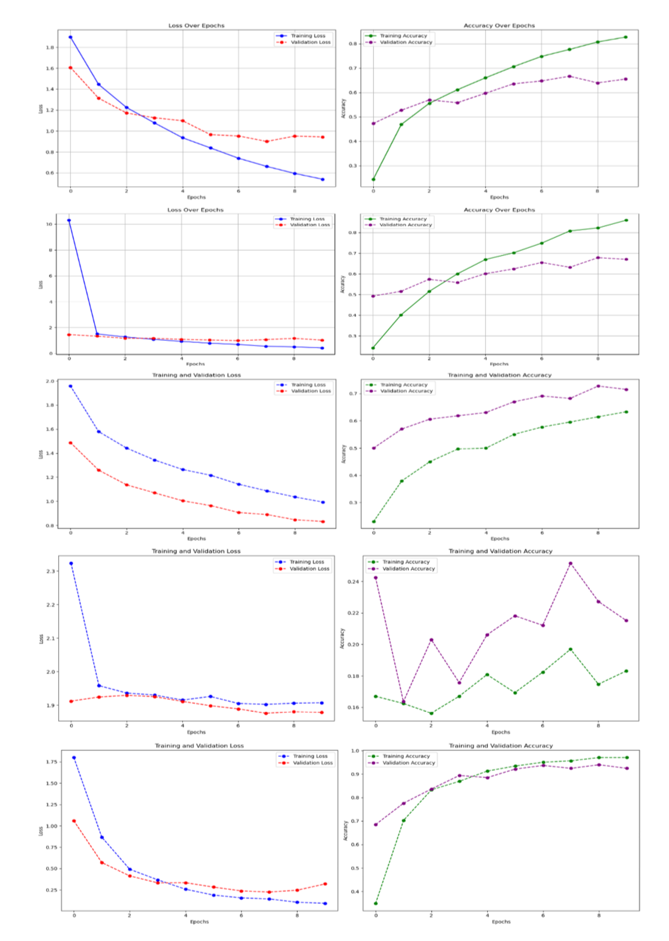
Figure 5. Training and validation curves for all five models on the Original_Normal_Grey_LT_190 subset of the 100 species dataset. (a) Baseline CNN, (b) Improved CNN, (c) VGG16, (d) ResNet50, (e) DenseNet121. The curves show loss and accuracy over epochs, demonstrating convergence patterns and potential overfitting indicators.

4.4. Grad-CAM Visualization Analysis

Figure 6. Grad-CAM heatmap visualizations for each model on representative plant images from the 100 species dataset. Each row shows: original image, Grad-CAM heatmap, and heatmap overlay. (a) Baseline CNN, (b) Improved CNN, (c) VGG16, (d) ResNet50, (e) DenseNet121. The visualizations demonstrate consistent emphasis on light-colored plant features across all models.

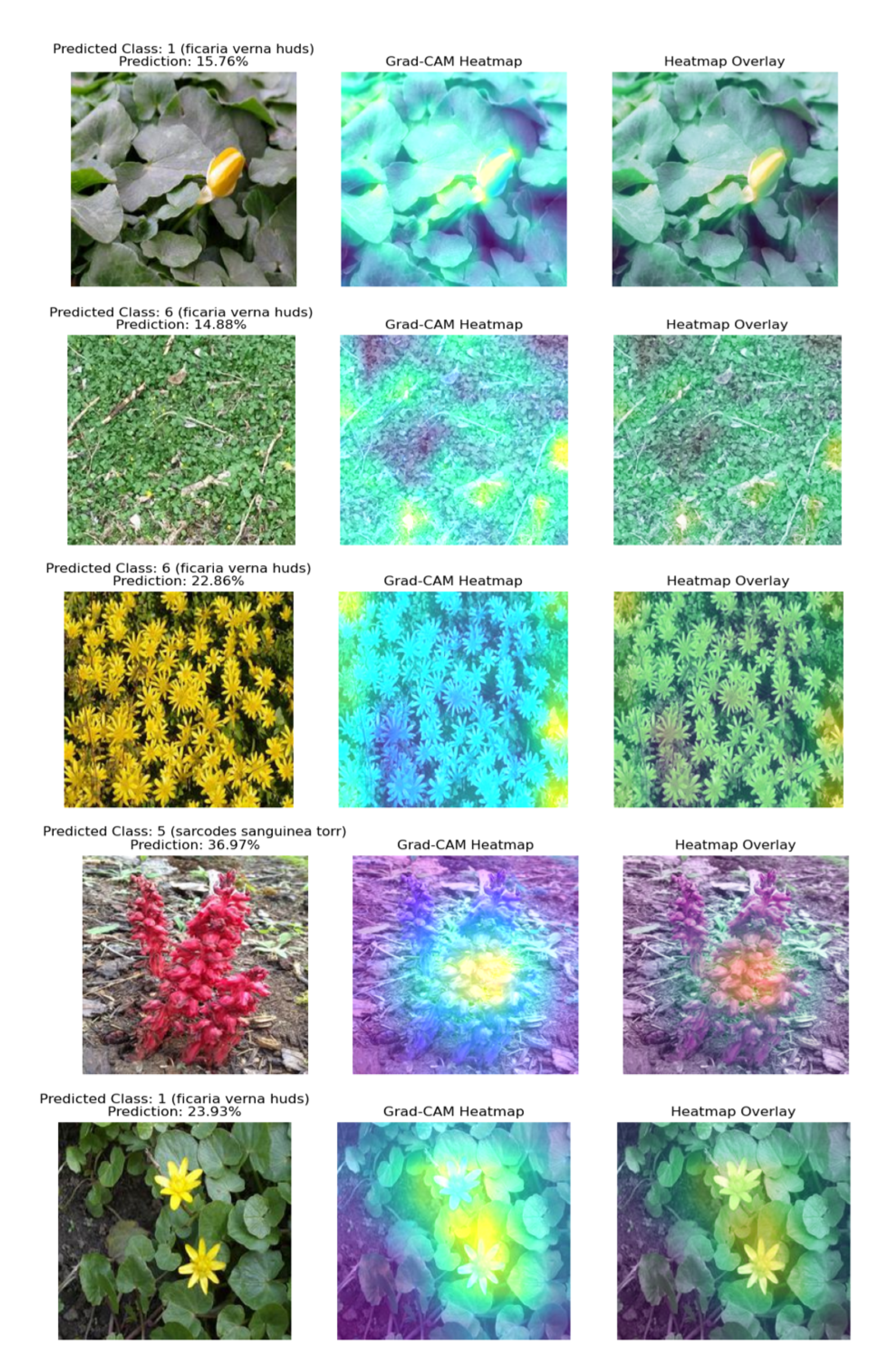
Figure 6. Grad-CAM heatmap visualizations for each model on representative plant images from the 100 species dataset. Each row shows: original image, Grad-CAM heatmap, and heatmap overlay. (a) Baseline CNN, (b) Improved CNN, (c) VGG16, (d) ResNet50, (e) DenseNet121. The visualizations demonstrate consistent emphasis on light-colored plant features across all models.

4.5. Greyscale Analysis Results

For comparison, we also analyzed model performance on greyscale versions of the datasets to understand color dependency.

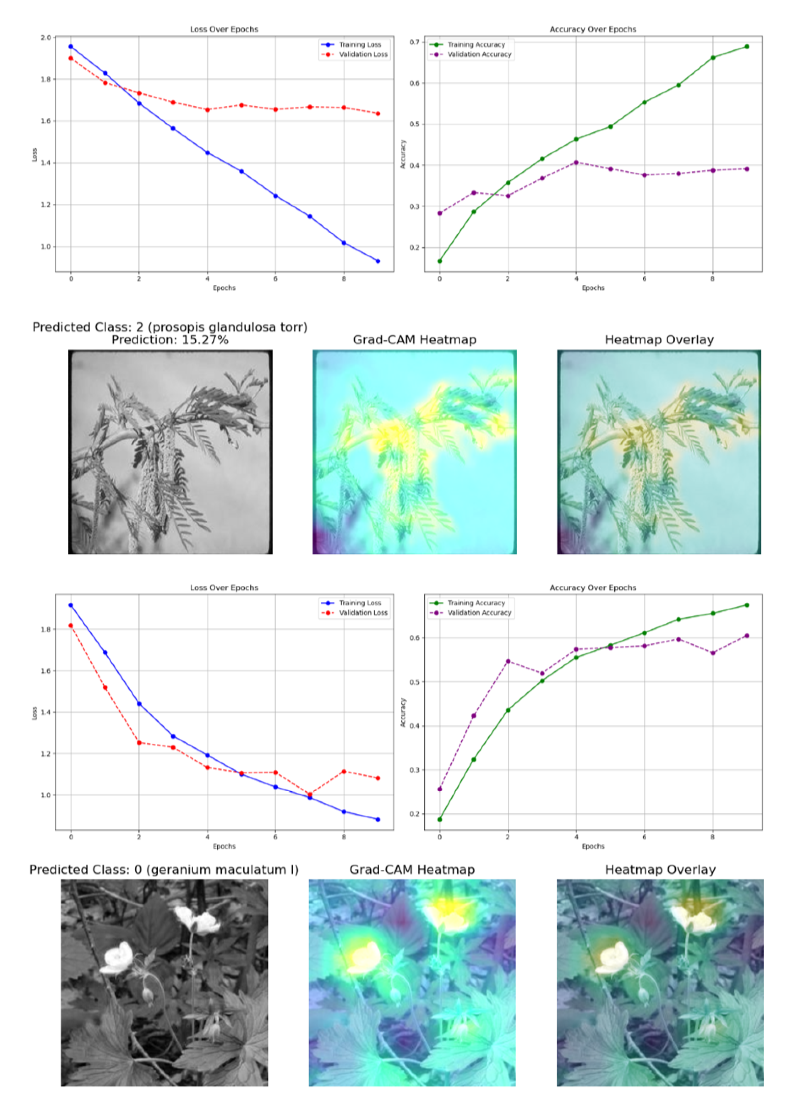
Figure 7. Comparative analysis of Baseline and Improved CNN models on greyscale versions of the Normal_Grey_LT_190 dataset. (a) Training curves for Baseline CNN, (b) Training curves for Improved CNN, along with corresponding Grad-CAM visualizations showing reduced but persistent bias patterns.

Figure 7. Comparative analysis of Baseline and Improved CNN models on greyscale versions of the Normal_Grey_LT_190 dataset. (a) Training curves for Baseline CNN, (b) Training curves for Improved CNN, along with corresponding Grad-CAM visualizations showing reduced but persistent bias patterns.

4.6. 30 Species Dataset Analysis

Figure 8. Training and validation curves for all five models on the complete 30 species dataset. (a) Baseline CNN, (b) Improved CNN, (c) VGG16, (d) ResNet50, (e) DenseNet121. The curves demonstrate generally improved performance compared to the 100 species dataset due to more uniform class distribution.

Figure 8. Training and validation curves for all five models on the complete 30 species dataset. (a) Baseline CNN, (b) Improved CNN, (c) VGG16, (d) ResNet50, (e) DenseNet121. The curves demonstrate generally improved performance compared to the 100 species dataset due to more uniform class distribution.

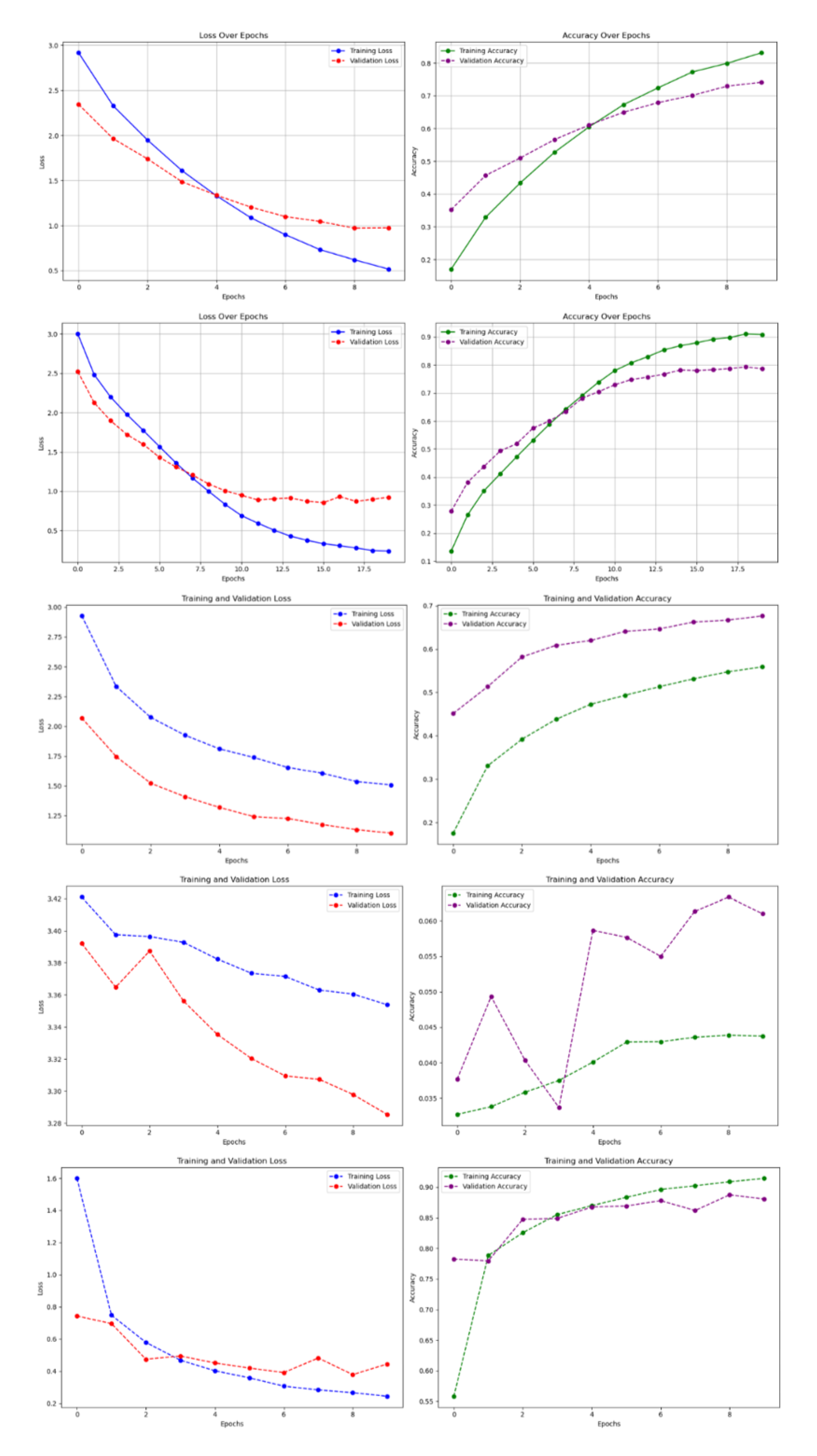
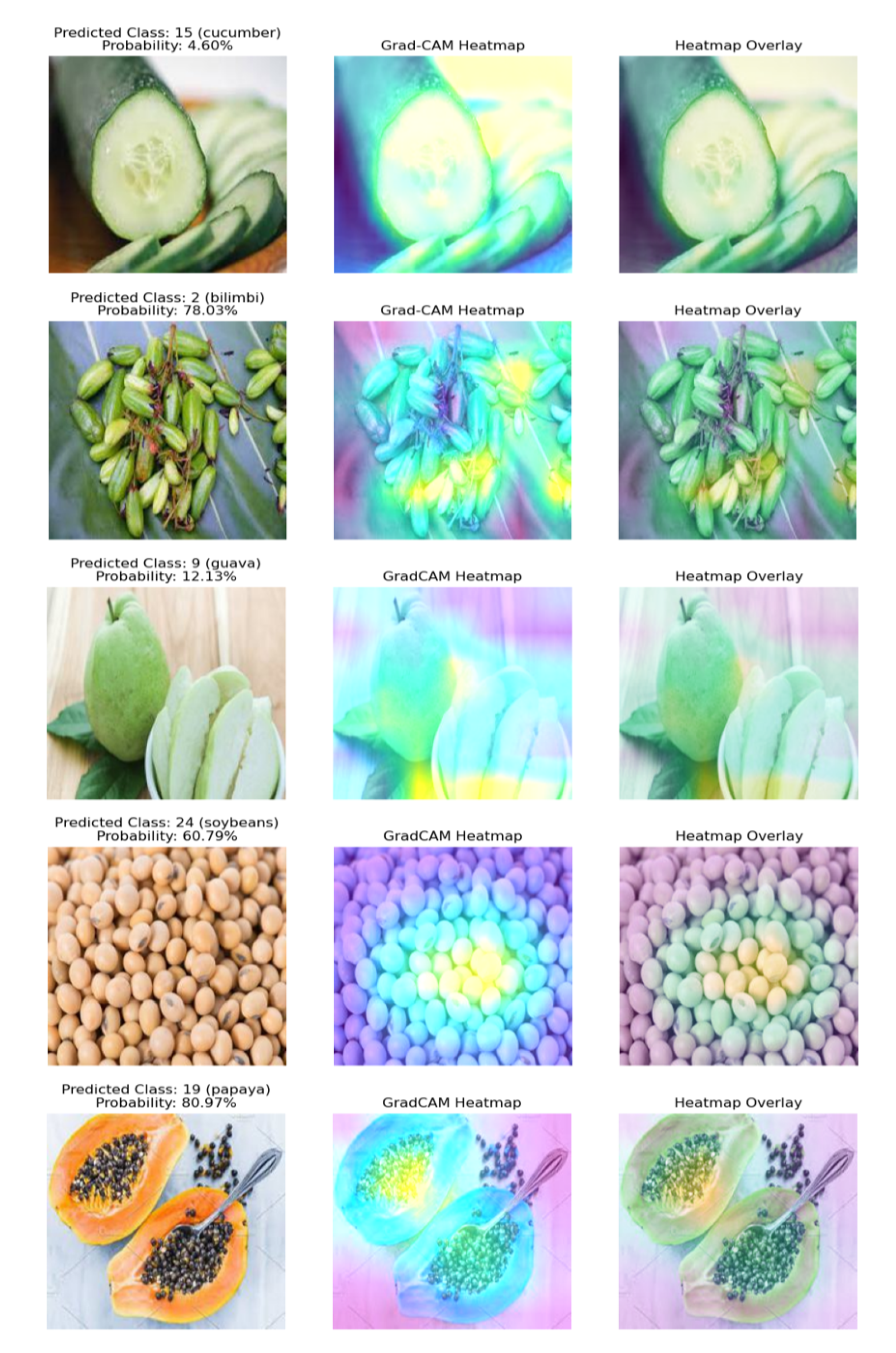
Figure 9. Grad-CAM visualizations for each model on representative images from the 30 species dataset. Examples include cucumber, papaya, soybeans, and other species, demonstrating the persistent light-color bias across different plant types and model architectures.

Figure 9. Grad-CAM visualizations for each model on representative images from the 30 species dataset. Examples include cucumber, papaya, soybeans, and other species, demonstrating the persistent light-color bias across different plant types and model architectures.

5. Discussion

For the 100 plant species dataset, DenseNet121 outperformed other models with an average accuracy of 80.70%, followed by VGG16 model (51.68%), while ResNet50 model was the least performing with an accuracy of 15.09%. Performing the same analysis for greyscale images did not improve model performance, with accuracy around 51.34%.

For the 30 plant species dataset, the DenseNet121 model (91.54%) was the best, followed by Baseline CNN (85.32%), VGG16 (83.57%), Improved CNN (82.87%), and ResNet50 model (44.05%) respectively.

In both datasets, the DenseNet121 model was the best, consistent with findings of Xiao et al. [25], who also found that pre-trained models are highly effective architectures for plant species classification. Moreover, the Baseline model also gave good results for the 30 plant species dataset, corresponding with Liu et al. [13], who achieved strong performance for their LtCNN model across different evaluation metrics like the kappa coefficient. This performance was possibly due to the larger number of images and more uniform distribution of plant species.

In understanding the model’s decision making using Grad-CAM, we observed that light colors, specifically colors closer to white as well as bright colors, were highlighted as significant features in Grad-CAM heatmaps. In their paper, Selvaraju et al. [20] also found that Grad-CAM is most effective at highlighting salient regions in images that contain these colors. For example, in the 100 plant species dataset, specifically the Original_Normal_Grey_LT_190 analysis, probability predictions show that ResNet50 (36.97%) model performed better, followed by DenseNet121 (23.93%), VGG16 (22.86%), Baseline CNN (15.76%) and Improved CNN (14.88%). This is inconsistent with their overall performance and could be because images with good performance had bright colors as significant features, as seen in the Grad-CAM visualizations. Additionally, in the 30 plant species dataset, predictions showed that DenseNet121 model (80.97%) was the best, then Improved CNN (78.03%), ResNet50 (60.79%), VGG16 (12.13%), and Baseline CNN model (4.60%). These inconsistencies could be due to bias towards light colors, thereby limiting effectiveness for plant species classification, as many plant species are not predominantly light-colored. For example, green plant species may not be well-represented in Grad-CAM heatmaps, as the algorithm is more sensitive to changes in color in green plant species than in other plant species.

6. Conclusions

The application of Explainable Artificial Intelligence (XAI) using Grad-CAM in the context of plant species classification with CNNs provided valuable insights into the decision-making processes of complex models. The use of Grad-CAM in visual explanations for decisions made by CNNs revealed interesting patterns. Notably, light colors, particularly those closer to white and bright hues, were consistently emphasized in Grad-CAM heatmaps. This finding aligned with previous research by Selvaraju et al. [20], confirming Grad-CAM’s effectiveness in highlighting salient regions in images containing such colors. However, this project also identified a potential limitation in Grad-CAM’s bias towards light-colored features, raising concerns about its effectiveness in accurately representing plant species that are not predominantly light-colored.

The integration of Grad-CAM as an XAI tool contributes to deeper understanding of CNN decision-making processes, with potential implications for improving model trustworthiness and addressing biases. Although XAI addresses challenges posed by the “black box” nature of deep learning models, especially in critical sectors such as healthcare, plant taxonomy, and security, where transparency and interpretability are paramount [12], further research needs to be done on Grad-CAM to mitigate its color bias if it is to be directly applied in these sectors. Additionally, exploring other visual explanatory tools such as LIME (Local Interpretable Model-agnostic Explanations), SHAP (SHapley Additive exPlanations), DeepLIFT (Deep Learning Important FeaTures), etc., could provide more comprehensive understanding of XAI.

References

- Adadi, A. and Berrada, M. (2018). Peeking inside the black-box: A survey on explainable artificial intelligence (xai). IEEE Access, 6:52138–52160. [CrossRef]
- Arrieta, A. B., Díaz-Rodríguez, N., Del Ser, J., Bennetot, A., Tabik, S., Barbado, A., García, S., Gil-López, S., Molina, D., and Benjamins, R. (2020). Explainable artificial intelligence (xai): Concepts, taxonomies, opportunities and challenges toward responsible ai. Information Fusion, 58:82–115. [CrossRef]
- Chen, T. and Guestrin, C. (2016). Xgboost: A scalable tree boosting system. In Proceedings of the 22nd ACM SIGKDD International Conference on Knowledge Discovery and Data Mining. [CrossRef]
- Doshi-Velez, F. and Kim, B. (2017). Towards a rigorous science of interpretable machine learning. arXiv preprint arXiv:1702.08608. arXiv:1702.08608. [CrossRef]
- Gilpin, L. H., Bau, D., Yuan, B. Z., Bajwa, A., Specter, M., and Kagal, L. (2018). Explaining explanations: An overview of interpretability of machine learning. In 2018 IEEE 5th International Conference on Data Science and Advanced Analytics (DSAA). IEEE. [CrossRef]
- Goodman, B. and Flaxman, S. (2017). European union regulations on algorithmic decision-making and a “right to explanation”. AI Magazine, 38(3):50–57. [CrossRef]
- Guidotti, R., Monreale, A., Ruggieri, S., Turini, F., Giannotti, F., and Pedreschi, D. (2018). A survey of methods for explaining black box models. ACM Computing Surveys (CSUR), 51(5):1–42. [CrossRef]
- Gunning, D., Stefik, M., Choi, J., Miller, T., Stumpf, S., and Yang, G. (2019). Xai—explainable artificial intelligence. Science Robotics, 4(37):eaay7120. [CrossRef]
- Joly, A., Müller, H., Goëau, H., Glotin, H., Spampinato, C., Rauber, A., Bonnet, P., Vellinga, W., and Fisher, B. (2014). Lifeclef: Multimedia life species identification. EMR: Environmental Multimedia Retrieval. [CrossRef]
- Jordan, M. I. and Mitchell, T. M. (2015). Machine learning: Trends, perspectives, and prospects. Science, 349(6245):255–260. [CrossRef]
- LeCun, Y., Bengio, Y., and Hinton, G. (2015). Deep learning. Nature, 521(7553):436–444. [CrossRef]
- Lipton, Z. C. (2018). The mythos of model interpretability: In machine learning, the concept of interpretability is both important and slippery. Queue, 16(3):31–57. [CrossRef]
- Liu, K., Yang, M., Huang, S., and Lin, C. (2022). Plant species classification based on hyperspectral imaging via a lightweight convolutional neural network model. Frontiers in Plant Science, 13:855660. [CrossRef]
- Miller, T. (2019). Explanation in artificial intelligence: Insights from the social sciences. Artificial Intelligence, 267:1–38. [CrossRef]
- Murdoch, W. J., Singh, C., Kumbier, K., Abbasi-Asl, R., and Yu, B. (2019). Definitions, methods, and applications in interpretable machine learning. Proceedings of the National Academy of Sciences, 116(44):22071–22080. [CrossRef]
- Pimm, S. L., Jenkins, C. N., Abell, R., Brooks, T. M., Gittleman, J. L., Joppa, L. N., Raven, P. H., Roberts, C. M., and Sexton, J. O. (2014). The biodiversity of species and their rates of extinction, distribution, and protection. Science, 344(6187):1246752. [CrossRef]
- Polikar, R. (2012). Ensemble learning. Ensemble Machine Learning: Methods and Applications, pages 1–34. [CrossRef]
- Saad, S. A. (2023). plant-species. Kaggle. Available at: https://www.kaggle.com/datasets/syedabdullahsaad/plant-species?resource=download (Accessed 2023-09-25).
- Safavian, S. R. and Landgrebe, D. (1991). A survey of decision tree classifier methodology. IEEE Transactions on Systems, Man, and Cybernetics, 21(3):660–674. [CrossRef]
- Selvaraju, R. R., Cogswell, M., Das, A., Vedantam, R., Parikh, D., and Batra, D. (2017). Grad-cam: Visual explanations from deep networks via gradient-based localization. In Proceedings of the IEEE international conference on computer vision. [CrossRef]
- Sulistya, Y. I. (2023). plants-type-datasets. Kaggle. Available at: https://www.kaggle.com/datasets/yudhaislamisulistya/plants-type-datasets/ (Accessed 2023-10-30).
- Wäldchen, J. and Mäder, P. (2018). Plant species identification using computer vision techniques: A systematic literature review. Archives of Computational Methods in Engineering, 25:507–543. [CrossRef]
- Wäldchen, J., Rzanny, M., Seeland, M., and Mäder, P. (2018). Automated plant species identification—trends and future directions. PLoS Computational Biology, 14(4):e1005993. [CrossRef]
- West, D. M. (2018). The future of work: Robots, AI, and automation. Brookings Institution Press.
- Xiao, Q., Li, G., Xie, L., and Chen, Q. (2018). Real-world plant species identification based on deep convolutional neural networks and visual attention. Ecological Informatics, 48:117–124. [CrossRef]
- Zhu, J., Liapis, A., Risi, S., Bidarra, R., and Youngblood, G. M. (2018). Explainable ai for designers: A human-centered perspective on mixed-initiative co-creation. In 2018 IEEE Conference on Computational Intelligence and Games (CIG). IEEE. [CrossRef]
Disclaimer/Publisher’s Note: The statements, opinions and data contained in all publications are solely those of the individual author(s) and contributor(s) and not of MDPI and/or the editor(s). MDPI and/or the editor(s) disclaim responsibility for any injury to people or property resulting from any ideas, methods, instructions or products referred to in the content. |
© 2025 by the authors. Licensee MDPI, Basel, Switzerland. This article is an open access article distributed under the terms and conditions of the Creative Commons Attribution (CC BY) license (http://creativecommons.org/licenses/by/4.0/).
Copyright: This open access article is published under a Creative Commons CC BY 4.0 license, which permit the free download, distribution, and reuse, provided that the author and preprint are cited in any reuse.