Submitted:
30 September 2025
Posted:
01 October 2025
You are already at the latest version
Abstract
We present a model of the human walking based on the well known model of double pendulum moving in a plane under the influence of gravity. For constructing the pendulum we use data for the average value of masses of the thigh and shank, as well as for their inertial moments, centers of masses and densities taken from a representative study of the Bulgarian males. We derived the corresponding differential equations governing the model and solved them numerically. We have shown that for moderate initial values of the angles and the angular velocities, describing the system, one has a regular reasonably looking movement of the pendulum resembling that one of the actual walking of humans.
Keywords:
double pendulum
; nonlinear dynamics
; nonlinear differential equations
; biomechanics
; chaos
; phase diagram
; numerical methods
; mass-inertial parameters of the human body
; mathematical modeling of the human body
1. Introduction
The plane double gravitational pendulum serves as a valuable model for understanding the complexities arising from nonlinearity in physical systems. The system’s behavior is described by a set of coupled, nonlinear, second-order differential equations that defy analytical solution [1]. Numerical simulation provides a powerful tool for exploring its dynamics, but requires careful attention to numerical errors and energy conservation. The double pendulum’s sensitivity to initial conditions and its chaotic nature underscore the limitations of long-term predictability in nonlinear systems. Visualization tools, such as animations and phase space plots, are crucial for analyzing and interpreting the simulation results [2]. In addition to numerically solving the equations we have also used these methods. The numerical exploration of the double pendulum’s dynamics reveals its most compelling characteristic: its sensitivity to initial conditions. This sensitivity, a hallmark of chaotic systems, means that infinitesimally small differences in the initial angles or velocities of the pendulums can lead to essentially different trajectories over time [3,4]. The chaotic nature of the double pendulum can be most appealingly visualized through phase space plots. These plots, which map the system’s state over time, reveal intricate and often fractal-like structures. Unlike simpler systems with predictable periodic motion that result in closed, repeating loops in phase space, the double pendulum exhibits trajectories that wander seemingly randomly through the phase space, never repeating themselves exactly. This behavior highlights the system’s inherent unpredictability and its departure from the predictable dynamics of linear systems.
The current article demonstrates that it can be helpful in matters of biomechanics, which is related to the problems of human walking. We show that within the typical range and parameters of the human motion the double pendulum behaves relatively regularly and does not have essential chaotic behavior.
The pendulum systems are classical models of nonlinear dynamics [5]. We would like to stress that, generally, the study of the double pendulum is not merely an academic exercise; it holds significance in various scientific and engineering fields [6,7,8,9,10,11,12,13]. Understanding its complexities aids in comprehending the dynamics of multi-body systems, informing the design of robotic arms, satellite stabilization systems, financial modeling, and even contributing to our understanding of planetary motion. Furthermore, it turns helpful for apprehending questions related, as stated, to physics of human motion, and also climate modeling [14,15] (for which Edward Lorenz’s coined the famous term “butterfly effect”, in article titled “Deterministic Nonperiodic Flow” published in his 1963 paper in the Journal of the Atmospheric Sciences), fundamental physics, and even entertaining sport activities, like golf, namely for modeling the golf swing with double pendulums [16]. The understanding of coupled oscillators is crucial in analyzing the behavior of electrical circuits, mechanical vibrations, and even the rhythmic firing of neurons in the brain.
The planar double gravitational pendulum, a seemingly simple system composed of two pendulums connected in series and swinging under the influence of gravity, belies its deceptive simplicity. It embodies a profound intersection of classical mechanics, nonlinear dynamics, and chaos theory, serving as a potent example of how seemingly deterministic systems can exhibit highly unpredictable behavior. A large number of investigations, both theoretical and experimental, have been dedicated to the problem of determining the chaotic behavior of double pendulum [17,18,19].
2. The Model
In this section we describe a model of the limbs of the human body. In its simplest version the model represents a type of gravitational pendulum. They can be reduced to plane double or triple gravitational pendulum, i.e., we consider the corresponding limb of the human body to embrace two segments. Any of the branches of the pendulum are supposed to be axis symmetric and characterized by the corresponding densities , , where s is defined so that it unicly determines the position of the corresponding cross-section of the given branch of the combined.
Of course, we need to determine the Lagrangian of the system. For that we need to clarify what is the kinetic and potential energies of the system in terms of the properly defined variables - see Figure 1. For the total kinetic energy K we obtain consequently
where , are the kinetic energies of the segments. Thus, for one has
where is the set of allowed values of and is the area of the cross-section of segment 1 at position measured from the beginning of the segment. In what follows we will take the densities of a given segment to be uniform, i.e., . The last actually reflects the experimental situation - data for the mass densities of a given segment differ from segment to segment, but within the specific segment they are assumed homogeneous. Then, taking into account that
and that
we immediately obtain
and, therefore
which leads to
Here
is a moment of inertia of segment “1” about an axes perpendicular to it and centered at its top. We have assumed that the length of the segment is .
Now we shall deal with the kinetic energy of the second segment in the limb. Let is the coordinate along the second segment. Then, looking at the geometry one derives
which leads to
and, therefore, to
Using the above expressions, for the kinetic energy we derive, consequently:
where ,
Obviously, is the coordinate of the center of mass of the second segment measured from its beginning.
Summarizing the above, we conclude that, if the limb consists of just two segments, its total kinetic energy equals to
Now we turn to the potential energy of the system V supposing the bodies to be acted upon by the gravity field of the Earth. Obviously
where and are the potential energies of the segments. From the geometry depicted in Figure 1 one has
where
In a similar way, for one derives
From Equations (18) and (20) we arrive at
Once we know the kinetic K and the potential V energies, we derive the Lagrangian of the system
One can also determine the Hamiltonian of the system
Since we did not introduce explicit dependence on the time t, the Hamiltonian of the system is conserved and equal to the stationary energy of the system. According to the standard Hamiltonian formulation, the state of a system is characterized not only by its positions (generalized coordinates) and , but also by its momenta and . Hence, the Hamiltonian of the system depicted in Figure 1 is:
where
3. The Equations of Motion
From Equation (22) one obtains the corresponding Euler-Lagrange equations, governing the behavior of the two segments of the considered limb. According to the general theory the equation are to be obtained from
In this way we obtain a set of two coupled, second-order, nonlinear differential equations:
and
Equation (27) can be rewritten in the simpler form
Equations (28) and (29) form the system of two coupled nonlinear differential equations. When modeling the process of walking one shall keep in mind that , when .
In the form of a dynamical model this system is
where
The data needed for the evaluation of the above quantities in case of human body are presented in Table 1 on the example of the average Bulgarian males. The data are taken from Ref. [20]. There, actually, the relative location of the center of mass of the body segments are given, but the transformation to physical lengths is trivial. In Ref. [20] one provides data for principal moments of inertia and , where the coordinate system is centered at the center of mass of the corresponding segment; the z axes is along the segment, while x and y axes for a plane orthogonal to it. Due to the supposed there symmetry, . One way of acting, in order to determine and is that they are equal to
where we are using the Steiner’s theorem. Another, direct approach is to recall that the thigh and shank are modeled there as frustum of cones and to derive that for the segment one has
Let us perform dimensional analysis for the quantities shown in Equation (31). One has that . Then , , , and , i.e., these constants are dimensionless. Finally, and . We have also to take into account that .
4. Biomechanical Data
In order to apply Equation (33), we have to take into account that, according to Ref. [21], for the thigh while for the shank .
The human gait is usually considered as a cycle decomposed into eight phases, see Figure 2. The phases can be categorized in various ways. Here we do that by using the ankles for the hip, knee, and ankle joint, for each of the eight phases of the human gait cycle. The angles are given, i.e. their typical values, in Table 2.
5. Numerical Results
The small free oscillations of a conservative linear system in the phase portrait have the form of closed trajectories in the neighborhood of a stable steady state. It is well-known that amplitudes of oscillations for linear systems (for nonlinear conservative ones also) depend on the initial conditions. On the other hand, its period is permanent and independent of initial conditions and the energy level of the system. The periodic oscillations in conservative systems are always orbitally stable, i.e. for very small perturbations in the initial conditions a periodical motion passes into another one as these two motions are very close. Solving numerically Equation (30) we obtain:
- 1)
- For small initial angles and speeds we obtain the following solutions for and :
- 2)
- For intermediate initial angles and speeds we obtain the following solutions for and :
Figure 3.
(a) The figure shows the behavior of and for and a specific choice of the initial conditions: , , , .(b) Phase diagram of the system under the same boundary conditions.
Figure 3.
(a) The figure shows the behavior of and for and a specific choice of the initial conditions: , , , .(b) Phase diagram of the system under the same boundary conditions.
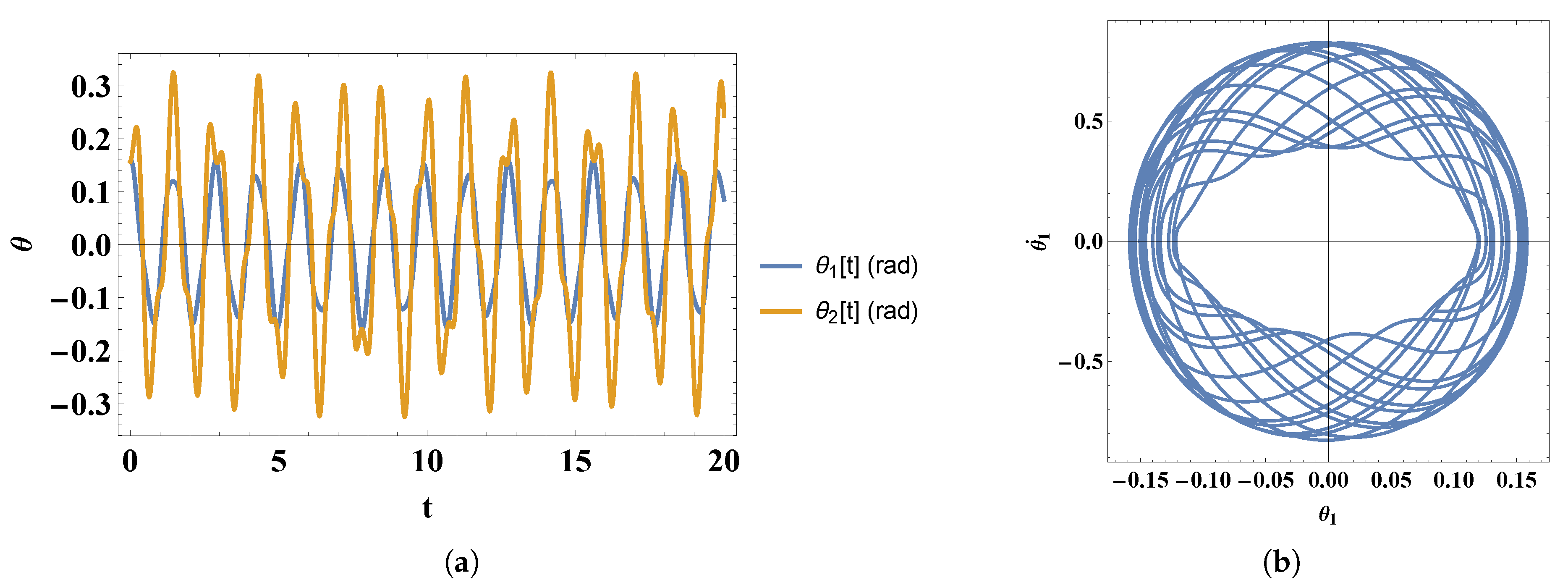
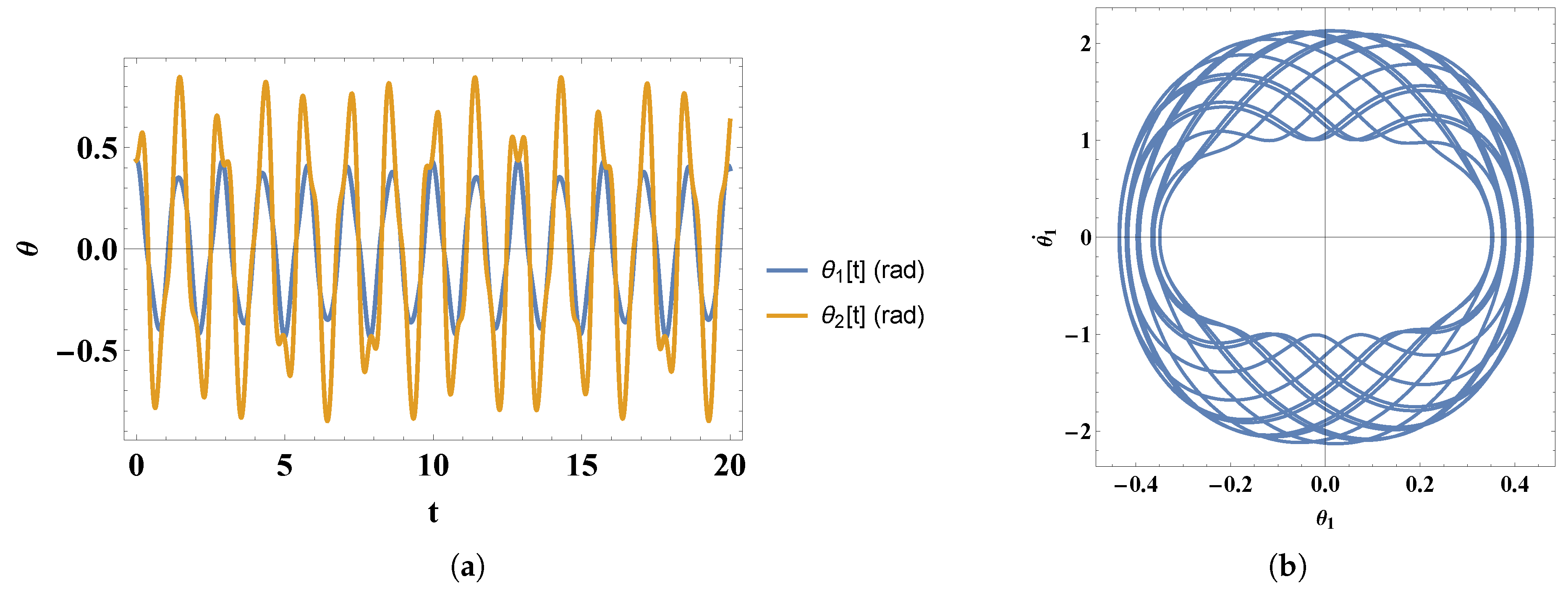
Figure 4.
(a) The figure shows the behavior of and for and a specific choice of the initial conditions: , , , . (b) Phase diagram of the system under the same boundary conditions. It demonstrates that the movement is not purely periodic but there is also an element of chaos in it. We observe that the spread of the phase diagram is about three times larger than for the small angles. i.e., larger the initial angles larger is the spread of the phase diagram.
6. Small Angles Approximation
In the current section we solve both analytically and numerically Equation (28) and Equation (29) form the system of two coupled nonlinear differential equations in the small angles approximation. Performing small angles expansion in these equation and retaining only linear terms, we obtain
and
Obviously, these two equations describe two linearly coupled oscillators. Looking for a solution in the form
we obtain
and
Plugging in Equation (39) and Equation (40) the values of all quantities involved, we obtain
The behavior of and is shown in Figure 5. One observes for very small angles periodic behavior. The changes in the behaviors of and are in phase with each other.
7. Comparison of Our Model Results to Real Walking
In this section, we will briefly discuss how our results compare to real walking. Walking is a fundamental human activity, essential for daily life, work, and social interaction. Its significance extends to well-being, enabling shopping, commuting, and maintaining connections with others. The study of human motion, with a particular focus on gait, has a long history, dating back to ancient times [23]. This research encompasses diverse areas, including neuromuscular disorders, joint replacement, sports injuries, and assistive devices [24,25]. Furthermore, the increasing interest in humanoid and wearable robots [26] underscores the continuing importance of understanding human locomotion. The results of our model of human walking indicate that for small initial angles (periodic movement), the period seconds. One forward swing of the leg corresponds to a half cycle, which takes s. This is quite close to the number reported in Ref. [27,28], according to which at slow walk s. s corresponds to about 2400 step/hour. If we assume the average step length to be approximately m, we obtain a speed of approximately km/h. For the movements shown in Figure 3, s, while for Figure 4, s. These data correspond to km/h and km/h, respectively. The corresponding step lengths are, then, . Having that for s one has we obtain for the step length m and m for s. According to Ref. [28] [p. 127], see also Refs. [29,30], the speed for a slow walk is about km/h. There one takes a step length of m, the time for a step s. For a fast walk, the speed is estimated about km/h, and the step length of about, m, so the step time is about s. As we see all these numbers are very close to the numbers we obtained within our model.
8. Conclusions
The mathematical model described in the current article is based on a double pendulum representation of a limb (e.g., thigh + shank) with realistic mass–inertia parameters. The model uses measured anthropometric data (those for average Bulgarian males in the paper). Naturally, it can be tailored to specific populations or individuals, making it a bridge between abstract physics and personalized bio-mechanical solutions. Thus, although it’s a theoretical construct, it has clear real-world applications across several domains: i) gait analysis and rehabilitation; The model can simulate normal and pathological walking patterns, helping clinicians design targeted physiotherapy or post-surgery recovery plans. ii) prosthetics and orthotics design; By adjusting parameters (mass, length, inertia) to match a patient’s anatomy, engineers can optimize artificial limbs for more natural movement. iii) injury prevention; Understanding joint loads and motion dynamics can guide ergonomic recommendations for athletes and workers. Many of the biomechanical problems associated with the evolution of total knee and total hip replacements have been evaluated in terms of walking mechanics. Mathematical modeling of human walking is an approach to estimate the human joint kinematics and dynamics during walking. More specifically, mathematical modeling and analysis help us distinguish between healthy patterns and the presence of any pathological alterations. Summarizing, we conclude that in the current paper, a realistic mathematical model of human limb movement is proposed using a double pendulum that moves in a plane under the influence of gravity. The model simulates the complete limbs of the human body and can easily be scaled to study different groups (children, women and et al.) of human populations. The model is dynamic, and it has a realistic representation, such as a slow/fast healthy walk. The model can be, obviously, improved by introducing torques acting on the segments of the pendulum. This will lead to source terms on the right-hand side of Equation (28) and Equation (29). The problem will become even more interesting and complicated if these torques depend on the time [31]. Understanding torques enables inferences about the muscles that most likely contract at certain moments to cause the leg to swing in tandem with gravity [24]. In addition, one can also consider a double inverted pendulum [32,33,34,35]. As already stated above, the key characteristic of the model is its non-linearity and chaos. Small changes in initial conditions can lead to different outcomes. This makes it a powerful model for studying the complex control required for human movement [9,31,36]. The double pendulum is a cornerstone model for understanding how the human body moves, as it perfectly illustrates the mechanics of multi-segment chains. Much of our gait (walking/running) can be explained by passive pendulum-like motion, which is incredibly energy-efficient. The model helps us understand this: indeed, during the swing phase of walking or running, the leg behaves remarkably like a double pendulum.
Author Contributions
Conceptualization, D.D., S.N. and G.N.; methodology, D.D., S.N. and G.N.; software, D.D.; validation, D.D., S.N. and G.N.; formal analysis, D.D. and S.N.; investigation, D.D., S.N. and G.N.; resources, D.D., S.N. and G.N.; data curation, G.N; writing—original draft preparation, D.D. and G.N.; writing—review and editing, D.D., S.N. and G.N.; visualization, D.D.; All authors have read and agreed to the published version of the manuscript.
Funding
This work is supported by Grant KP-06-H72/5, competition for financial support for basic research projects—2023, Bulgarian National Science Fund.
Data Availability Statement
No new data were created in the current article.
Acknowledgments
This work was accomplished by the Center of Competence for Mechatronics and Clean Technologies “Mechatronics, Innovation, Robotics, Automation and Clean Technologies” – MIRACle, with the financial support of contract No. BG16RFPR002-1.014-0019-C01, funded by the European Regional Development Fund (ERDF) through the Programme “Research, Innovation and Digitalisation for Smart Transformation” (PRIDST) 2021–2027.
Conflicts of Interest
The authors declare no conflicts of interest.
References
- Ott, E. Chaos in dynamical systems; Cambridge university press, 2002.
- Rose, J.; Gamble, J.G. Human walking. Philadelphia 2006. [Google Scholar]
- Kim, S.Y.; Hu, B. Bifurcations and transitions to chaos in an inverted pendulum. Phys. Rev. E 1998, 58, 3028. [Google Scholar] [CrossRef]
- DeSerio, R. Chaotic pendulum: The complete attractor. Am. J. of Phys. 2003, 71, 250–257. [Google Scholar] [CrossRef]
- Nayfeh, A.H.; Mook, D.T. Nonlinear oscillations; John Wiley & Sons, 2024.
- Strogatz, S.H. Nonlinear Dynamics and Chaos: With Applications to Physics, Biology, Chemistry, and Engineering; Chapman and Hall/CRC, 2024. [CrossRef]
- Ardema, M.D. Analytical dynamics: theory and applications; Springer Science & Business Media, 2005.
- Guckenheimer, J.; Holmes, P. Nonlinear oscillations, dynamical systems, and bifurcations of vector fields; Vol. 42, Springer Science & Business Media, 2013.
- Baker, G.L.; Blackburn, J.A. The pendulum: a case study in physics; OUP Oxford, 2008.
- Dutra, M.S.; de Pina Filho, A.C.; Romano, V.F. Modeling of a bipedal locomotor using coupled nonlinear oscillators of Van der Pol. Biological Cybernetics 2003, 88, 286–292. [Google Scholar] [CrossRef]
- Nikolov, S.G.; Vassilev, V.M.; Zaharieva, D.T. Analysis of swing oscillatory motion. In Proceedings of the Annual Meeting of the Bulgarian Section of SIAM. Springer; 2018; pp. 313–323. [Google Scholar]
- Nikolov, S.; Zaharieva, D. Dynamical behaviour of a compound elastic pendulum. In Proceedings of the MATEC Web of Conferences. EDP Sciences, Vol. 145; 2018; p. 01003. [Google Scholar]
- Arnold, V.I. Geometrical methods in the theory of ordinary differential equations; Vol. 250, Springer Science & Business Media, 2012.
- Baines, P.G. Lorenz, EN 1963: Deterministic nonperiodic flow. Journal of the Atmospheric Sciences 20, 130–41.1. Progress in Physical Geography 2008, 32, 475–480. [Google Scholar] [CrossRef]
- Lorenz, E.N. Deterministic nonperiodic flow 1. In Universality in Chaos, 2nd edition; Routledge, 2017; pp. 367–378.
- Penner, A.R. The physics of golf. Reports on progress in physics 2002, 66, 131. [Google Scholar] [CrossRef]
- Shinbrot, T.; Grebogi, C.; Wisdom, J.; Yorke, J.A. Chaos in a double pendulum. American Journal of Physics 1992, 60, 491–499. [Google Scholar] [CrossRef]
- Levien, R.; Tan, S. Double pendulum: An experiment in chaos. American Journal of Physics 1993, 61, 1038–1038. [Google Scholar] [CrossRef]
- Komuro, M. Double pendulum and chaos. Journal of the Robotics Society of Japan 1997, 15, 1104–1109. [Google Scholar] [CrossRef]
- Nikolova, G.S.; Toshev, Y.E. Estimation of male and female body segment parameters of the Bulgarian population using a 16-segmental mathematical model. Journal of biomechanics 2007, 40, 3700–3707. [Google Scholar] [CrossRef] [PubMed]
- Nikolova, G.; Kotev, V.; Dantchev, D.; Tsveov, M. Study of mass-inertial characteristics of female human body by walking. In Proceedings of the AIP Conference Proceedings. AIP Publishing LLC, Vol. 2239; 2020; p. 020032. [Google Scholar]
- Nikolova, G.; Dantchev, D.; Tsveov, M. Age changes of mass-inertial parameters of the female body by walking. Vibroengineering Procedia 2023, 50, 125–130. [Google Scholar] [CrossRef]
- Harris, G.F.; Smith, P.A.; et al. Human motion analysis: current applications and future directions. (No Title) 1996.
- Braune, W.; Fischer, O. The human gait; Springer Science & Business Media, 2012.
- Winter, D.A. Biomechanics and motor control of human movement; John wiley & sons, 2009.
- Asbeck, A.T.; De Rossi, S.M.; Galiana, I.; Ding, Y.; Walsh, C.J. Stronger, smarter, softer: next-generation wearable robots. IEEE Robotics & Automation Magazine 2014, 21, 22–33. [Google Scholar] [CrossRef]
- Herman, I.P. Physics of the human body; Springer, 2007.
- Herman, I.P. Physics of the human body; Springer, 2007. [CrossRef]
- Majed, L.; Ibrahim, R.; Lock, M.J.; Jabbour, G. Walking around the preferred speed: examination of metabolic, perceptual, spatiotemporal and stability parameters. Frontiers in physiology 2024, 15, 1357172. [Google Scholar] [CrossRef] [PubMed]
- Saibene, F.; Minetti, A.E. Biomechanical and physiological aspects of legged locomotion in humans. European journal of applied physiology 2003, 88, 297–316. [Google Scholar] [CrossRef] [PubMed]
- Chen, J. Chaos from simplicity: an introduction to the double pendulum 2008.
- Buczek, F.L.; Cooney, K.M.; Walker, M.R.; Rainbow, M.J.; Concha, M.C.; Sanders, J.O. Performance of an inverted pendulum model directly applied to normal human gait. Clinical Biomechanics 2006, 21, 288–296. [Google Scholar] [CrossRef] [PubMed]
- Colobert, B.; Crétual, A.; Allard, P.; Delamarche, P. Force-plate based computation of ankle and hip strategies from double-inverted pendulum model. Clinical biomechanics 2006, 21, 427–434. [Google Scholar] [CrossRef] [PubMed]
- Carroll, S.; Owen, J.S.; Hussein, M.F. Experimental identification of the lateral human–structure interaction mechanism and assessment of the inverted-pendulum biomechanical model. Journal of Sound and Vibration 2014, 333, 5865–5884. [Google Scholar] [CrossRef]
- Kuo, A.D. The six determinants of gait and the inverted pendulum analogy: A dynamic walking perspective. Human movement science 2007, 26, 617–656. [Google Scholar] [CrossRef] [PubMed]
- Morin, D. Introduction to classical mechanics: with problems and solutions; Cambridge University Press, 2008.
Figure 1.
The picture shows a simplified version of the model of either the upper limb, or of the lower limb.
Figure 1.
The picture shows a simplified version of the model of either the upper limb, or of the lower limb.
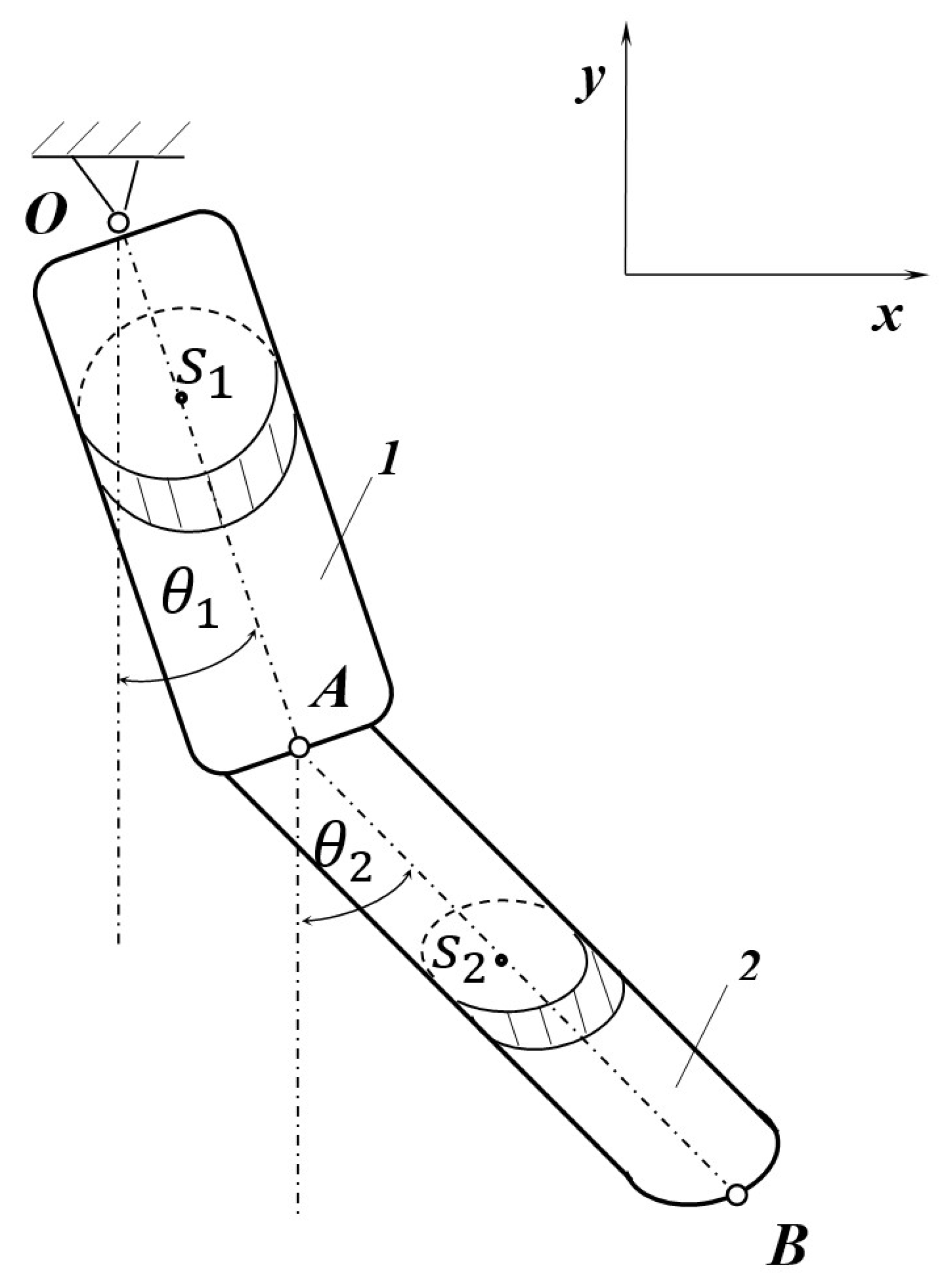
Figure 2.
The gait is typically thought of as a continuous series of periodic activities. The full gait cycle is normally defined as the time interval between the first heel strike contact of one foot (for example, the right foot) and the subsequent heel strike contact of the same foot. We use the so-called new gait terms involving the following eight phases, following one of the widely-accepted categorizations reported in the literature: 1) initial contact, 2) loading response, 3) midstance, 4) terminal stance, 5) pre swing, 6) initial swing, 7) mid swing, and 8) late swing, see Refs. [21,22]. All angles are measured with respect to the vertical axis passing trough the middle of the body, see Table 2.
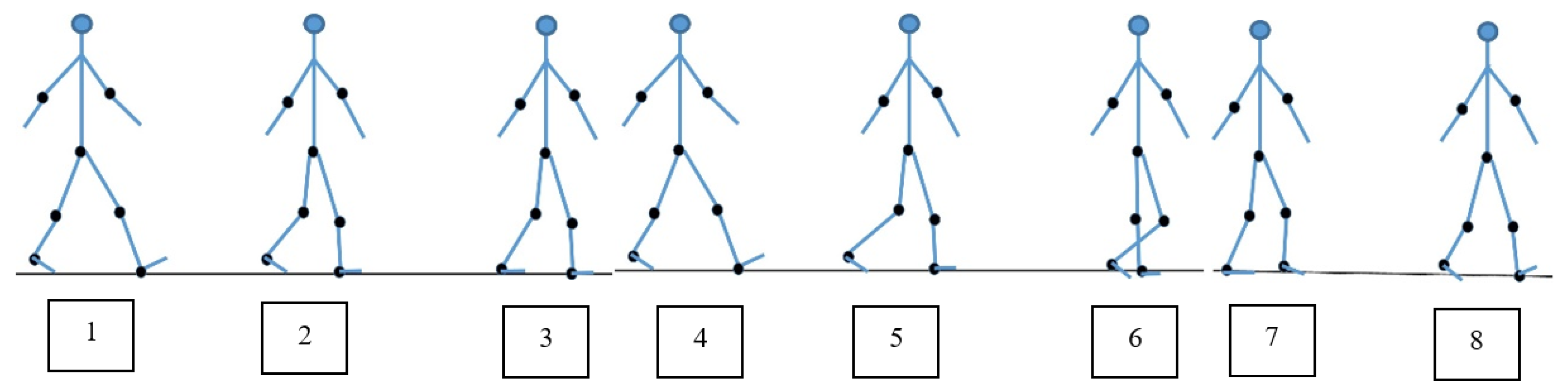
Figure 5.
The figure shows the behavior of and as a function of .
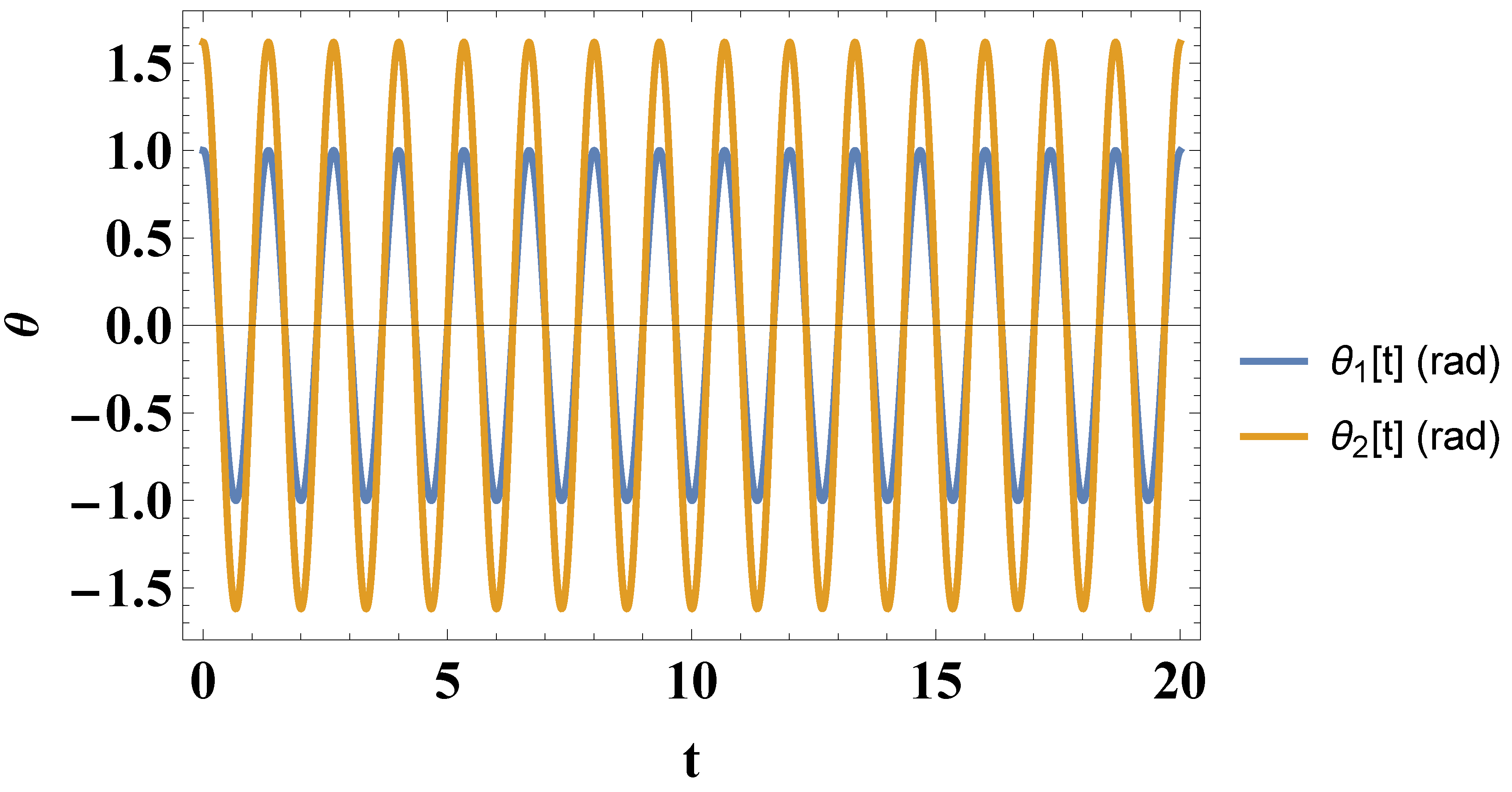

Table 1.
Geometric and mass-inertial characteristics of the thigh and shank of the average Bulgarian male.
Table 1.
Geometric and mass-inertial characteristics of the thigh and shank of the average Bulgarian male.
| Segment | Length ] | Mass [kg] | Centre of mass from the proximal end of the segment [ ] | Moments of inertia [] |
|---|---|---|---|---|
| Thigh | 51.0 | 11.0 | 21.1 |
= 6321.42 =1564.0 =1564.0 = 307.7 |
| Shank | 37.2 | 3.3 | 16.6 |
= 1124.3 = 231.9 =231.9 = 34.0 |
Table 2.
The table provides the hip, knee, and ankle joint angles for each of the eight phases of the human gait cycle.
Table 2.
The table provides the hip, knee, and ankle joint angles for each of the eight phases of the human gait cycle.
| Gait phases of the human gait cycle | Initial contact | Loading response | Mid stance | Terminal stance | Pre Swing | Initial Swing | Mid Swing | Terminal Swing |
|---|---|---|---|---|---|---|---|---|
| Hip | ||||||||
| Knee | ||||||||
| Ankle joint |
Disclaimer/Publisher’s Note: The statements, opinions and data contained in all publications are solely those of the individual author(s) and contributor(s) and not of MDPI and/or the editor(s). MDPI and/or the editor(s) disclaim responsibility for any injury to people or property resulting from any ideas, methods, instructions or products referred to in the content. |
© 2025 by the authors. Licensee MDPI, Basel, Switzerland. This article is an open access article distributed under the terms and conditions of the Creative Commons Attribution (CC BY) license (http://creativecommons.org/licenses/by/4.0/).
Copyright: This open access article is published under a Creative Commons CC BY 4.0 license, which permit the free download, distribution, and reuse, provided that the author and preprint are cited in any reuse.


