Submitted:
30 September 2025
Posted:
01 October 2025
You are already at the latest version
Abstract
Temporal variability in online streams arises in information systems where heterogeneous modalities exhibit varying latencies and delay distributions. Efficient synchronization strategies help to establish a reliable flow and ensure a correct delivery. In this paper, we establish a formal modeling foundation to address temporal dynamics in streams with multimodality using a discrete event system specification framework. This specification captures different latencies and interarrival dynamics inherent in multimodal flows. We also incorporate a Markov variant to account for variations in delay processes, thereby capturing timing uncertainty in a single modality. The proposed models are modular with inherent accounts for diverse temporal integration, thereby facilitating heterogeneity in information flows and communication. Various structural and behavioral forms can be flexibly represented and readily simulated. We demonstrate the experiments of several model permutations through the time-series behavior of individual stream components and the overall composed system, highlighting performance metrics in both, while quantifying the composability and modular effects.
Keywords:
multimodality
; information flow
; modeling & simulation
; diffusion
1. Introduction
Temporal multimodality provides new avenues for heterogeneous information processing. Efficient handling of such phenomena significantly enhances the ability to account for a wide range of diverse data types in unified platforms and environments. Recent artificial intelligence (AI) models [1,2,3] process multimodality in unprecedented ways, often quite natively using deep neural architectures [4,5]. From real-time language translations to reasoning over images and video processing and captioning, we expect the recent breakthroughs in recent models to drive a new future of products and innovations that utilize such advances.
Handling such diversity requires a foundation that lays the groundwork for various accounts in terms of forms and latencies. Especially in time-sensitive domains, the synchronization of different and time-varying forms needs to be constantly assessed to ensure a seamless flow with minimal discrepancies. The computational complexity of various new AI-driven solutions must be examined and thoroughly tested to select candidates that can offer potential improvements and novelty to traditional methods.
Thus, we formulate a computational foundation to simulate the information flow that inherently accommodates temporal multimodality. In such streams, different kinds of signals arrive with variable latencies, irregular timing, and delays. Combining methods across layers, from symbolic reasoning to signal processing, can be challenging due to interdisciplinary barriers. However, having a framework that enables such multilayered assessment by leveraging recent AI models (i.e., neural encoding and diffusion) stands to offer significant resolutions for widely known challenging issues.
Figure 1 illustrates how modern communications may take place given temporal multimodality. Various forms of inputs enter the pipeline through different ports and channels. Each form is sanctioned by a different latency. Additionally, jitter occurs during transmission, causing further variability in the flow due to the different latencies of each modality. The synchronization layer, therefore, must accommodate such variations. To effectively reconstruct the flow correctly, the layer utilizes a suitable AI model tailored to each modality for denoising. The final outcome is a correctly constructed stream according to a defined quality threshold.
Thus, we propose a simulation modeling framework to precisely account for the variability and jitter in multimodal flows. We model each modality as an incoming input into the system, characterized by distinct latency and jittering behavior. Each input encounters variable delays derived from a predetermined distribution. It simulates the varying latencies that each modality encounters, as well as the varying jitter that each latency may also undergo. Specific dropping semantics can also be introduced at this stage. At the synchronization layer, we implement a model that expects incoming inputs with various latencies and combines them to form the corresponding flow. At this layer, the model can be tuned to minimize waiting and optimize overall performance within a well-defined experimental framework.
We will provide background information about the underlying formulations in the next section. Then, Section 3 explains in detail our methodology in creating the modeling & simulation (M&S) framework in light of the given background. We then demonstrate our approach with example simulations and experiments in Section 4, and discuss the results in Section 5.
2. Background
In this section, we provide some necessary background information. We use the Discrete Event System Specification (DEVS) to formulate the layers and building blocks of the framework. We also draw on background using models of computation in addressing heterogeneous systems. We also use activity diagrams as an interface language to describe DEVS overall behavior before mapping them onto formal specification and execution. We also highlight some related backgrounds.
2.1. The DEVS Formalism
We utilize the DEVS formalism [6] to describe the overall architecture of the proposed system, featuring various layers that leverage the formalism’s expressiveness in terms of modularity and hierarchy. The formalism has been employed to guide the development of simulations in various domains, such as the Internet of Things [7] and cyberphysical system design [8]. We also use it to describe the basic building blocks (atomic models) to drive the computational execution of the simulation. Due to the unique combination of these two features, it is well-suited to modularize components with various temporal modalities. The coupled model in DEVS allows for the hierarchical construction of components. It does not describe the behavior of transition functions as in the atomic model. The coupled model may consist of sub-components (i.e., atomic and other coupled). It also consists of couplings, where external input coupling connects entry points to sub-components, external output coupling connects sub-components to exit points and ports, and internal coupling connects sub-components with each other according to a well-defined set of basic rules. The X and Y sets are used to handle the arrival of input and departure of output events, respectively.
The atomic model mainly defines the following. X and Y are the sets of inputs and outputs (I/O). S is the set of states with as an initial state. The external transition function handles the arrival of inputs and their effects on the model behavior by defining the state transition. The internal transition function works in a similar manner; however, it is triggered internally after elapsing , which is defined by the time advance function (ta). The output function defines how the model generates and emits outputs. It is triggered prior to calling . In parallel DEVS, acts as a select function to handle the confluence of and when it arises. , , and can include deterministic, probabilistic transitions, or both.
We use DEVS Markov [9] in particular to effectively simulate irregularities in temporal multimodal streams. We leverage the strong support for modularity in DEVS to construct multiple flows, components, layers, and levels within streams. We devise a DEVS-based architecture that enables capturing multimodalities and enables a time-based simulation of their streams with various distributions. The root coupled model represents the system in a modular manner, allowing for the observation of a wide range of performance and behavioral metrics while ensuring simulation correctness. We discuss the formulation details of the models and experiments in Section 3 and Section 4, respectively.
2.2. Activities and Other Related Background
We employ activity diagrams to intuitively describe the flow dynamics [10]. Previous research has employed DEVS as a foundation for modeling and simulating these diagrams [11]. In this work, we utilize activity abstraction to describe various flow logic in multimodal streams and use the predefined code generation facility to streamline the development of their corresponding simulation models. We also leverage the experimental frame [12] to initiate the execution and derive the performance metrics of interest. The dual-layer approach further ensures the correctness of the devised models and assists in the behavioral modeling and interpretation of simulation results.
The modal model is an actor model in Ptolemy [13] that primarily governs the transitions between different modes in systems. Our work relates to that notion in the way that the system may operate differently when passing through different modalities. In the example of passing inputs cleanly, as opposed to introducing Gaussian noise, the system exhibits heterogeneous behavior, as presented in the combined plot where two trajectories resulting from different modes are concatenated. In our approach, the composition of different time trajectories is achieved by deriving the results through coupling and via the experimental frame. Further refinement in the modal model is enabled through a hierarchical finite-state machine that dictates the system’s behavior.
Additionally, incorporating models of diffusion [14] is prompting a substantial shift in how traditional systems approach multimodality more broadly. Assessing the incorporation of various models through the synchronization layer provides a foundation for proper appropriation of these models in time-sensitive domains.
3. Methods
We first specify the model at a high level using an activity flow diagram. We represent each modality as an input parameter. Upon arrival, different modalities follow parallel paths with varying latencies and jitter specifications. Each path consists of atomic steps/actions with a distinct timing and state characterizations. Each action may optionally have a queue to manage multiple arrivals and input pressure. It can also be used to define dropping semantics. However, it is an optional feature for the model, and the flow may opt to lose inputs that arrive while actions are in a processing state. After completing these steps, each input modality ultimately reaches the synchronization node. Now, the underlying model allows for different combining mechanisms to take place with various accounts of timing, order, and types. For example, inputs received through different channels can be combined arbitrarily or according to a predefined mechanism. It can also be extended to accommodate a live stream and time windows.
The underlying formulation specifies the overall structure of the system with models, layers, hierarchical levels, and couplings. It also specifies the state transition and time advance functions of each atomic model. A generic overall structure of the model is depicted as an activity flow diagram in Figure 2. Horizontal layers highlight the stages through which the stream undergoes state changes, where hierarchical levels determine depth. We note that the diagram can be readily simulated, as we will describe the following stages.
The diagram is transformed into a fully specified coupled model. The coupled model consists of multiple atomic models. It is initially a one-level model. But we will later expand it further to cover more detailed cases with a multi-level hierarchy and examine its effect on the observed analytics. Each modality is represented in the coupled model as an external input to the root model. Each modality stream undergoes a distinct latency at the beginning, specified by an atomic model with a deterministic or probabilistic timing assignment and state changes. At the second stage of this layer, a new set of atomic models introduces the timing variability to the stream by using various distributions in a modular DEVS Markov model. It can be a single atomic model. But it can also consist of multiple models in various structural and hierarchical arrangements.
3.1. Synchronization and Denoising Layer
In this layer, we aim to describe how we handle multiple incoming flows that have been processed by the model over the previous stages. These flows are characterized by both deterministic and stochastic variations introduced along the stream. Now, the goal is to synchronize all these incoming flows into a unified flow. By doing so, we can reconstruct the output into a consistent stream. We may also rely on underlying mechanisms inside the model to assist with reconstruction and calibration, ensuring that the combined stream can proceed further and later be assessed by the transducer at the experimental frame.
In the model, we are essentially implementing multiple queues at the synchronization layer to handle a variety of inputs from different streams. We also implement different mechanisms to handle both the arrival and departure of elements within these queues.
Initially, these inputs may be treated arbitrarily, but we also introduce predefined ordering and matching mechanisms among the multimodal inputs in different queues. These mechanisms rely on timestamps or identity annotations that were added at earlier stages of the model and the generation process accordingly. The synchronization process ensures that inputs are aligned and merged in a coherent way. All of this can be specified within our model in a configurable manner, starting with some initial default assignments. In the experimental section of the paper, we will discuss an initial basic scenario and then demonstrate how changing configurations impact the results and analytics of the simulation.
3.2. DEVS Modeling
In this subsection, we formulate the entire DEVS specification in three steps. First, we establish the overall coupled model, which serves as the root model representing the overall architecture of the approach. We then proceed to creating templates for coupled models that represent each stream in a more modular and hierarchical manner. Finally, we lay the foundation and create templates for all the different types of atomic models as fundamental building blocks that run the executable simulation.
3.2.1. The Root Coupled Model
We organize the structure and hierarchy of the root model to capture the multiple layers horizontally. First, each modality is treated by a distinct external input port. Then, each layer is represented by a coupled model across the flow. Finally, an external output port represents the final stage at which the flow is directed to its ultimate destination. In the simulation experiment, this port is linked to the transducer model, from which the performance metrics are then derived. We formulate the root coupled model as follows:
Let there be i modalities . The root-level coupled model is
contains three coupled models representing each layer, that is, a delay layer , a jitter layer , and a synchronizer where:
Delay layer:
Each is represented by an atomic model with time advance (realizing ) and ports , . External couplings of are specified as:
Jitter layer:
Each is an atomic model with a time advance function that is drawn from a stochastic parametrization (e.g., specifying a delay distribution in DEVS Markov), ports , . External coupling of are specified as:
Synchronizer: With as an atomic model [11] that receives i number of inputs and dispatches a unified stream:
The remaining specification of the root coupled model follows:
External input couplings route each modality to its designated flow. External output coupling links the synchronizer output to the final destination while internal couplings establish the full flow for each modality.
3.2.2. Jitter Couplings
primarily consists of i models for representing jitter and dropping semantics for each modality flow. By leveraging hierarchy in DEVS Markov, each one of these models can be either an atomic or a coupled model. We formulate a generic coupled model to better capture stochastic behavior more broadly. The coupling of this newly formulated model with the root coupled model remains unchanged, preserving the original interface. That is, for :
Now, we further decompose the jitter model for each modality by formulating a coupled model as follows:
Each is an atomic model with a time advance function and transitions to specify various aspects of the model, such as random jitter and dropping conditions. Once each atomic model is specified, the couplings can be specified, forming a coupled, modular DEVS Markov system that can be readily simulated by a DEVS-compliant simulator.
The following describes the DEVS tuple of this atomic model generally:
with and .
We will describe more details about the inner functions in the following subsection. We now highlight that the constructed coupling essentially forms a graph [15] that mimics a directed acyclic graph, where nodes represent the atomic models and edges represent the couplings. In such a way, acts as a stochastic kernel inducing DEVS Markov modulation. As such, a function exists that maps an input arrival time at the port to a random output time at the port . For example, if consists of two atomic models in sequence where feeds , then the total delay distribution is obtained by the convolution of each individual distribution. Let and denote the nonnegative random variables associated with and respectively. Then the total delay is
with probability density
Therefore, the composed mapping of this particular kernel form is
where s is the input arrival time, u is the output departure time from and instantaneously entering , and t is the output departure time from and thereby .
In Section 4, we demonstrate the use of various DEVS Markov structures, as well as variations in processing and dropping semantics.
3.2.3. Atomic Models
We extend our formulation to specify three types of atomic models. The first type is a delayed action with an optional queue. The second one represents a decision point with a preassigned probability for dropping. The third one is for synchronizing the arrival of multiple streams. We will present the specifications of each model, with a particular focus on the external transition functions.
First, upon input arrival, an atomic model (action) specifies the time advance function that governs the transition to the next state and thereby generates the output. Each modality can be governed by a different distribution type. For example, an exponential distribution might be used with network packets and sensor data. More specific determinations using other distribution types might be more suitable with other forms of data and communication (e.g., video, acoustic). It can also be specified in a deterministic manner.
Thus, each deterministic/stochastic delay action is specified as an atomic DEVS
While the time advance function () is given by a random variable drawn from a distribution chosen according to the modality:
where is the delay distribution with typical parameterizations such that:
where each flow can be assigned to components specified according to the modular DEVS Markov variant with the appropriate parametrization for each form (e.g., audio, video, sensor feeds, heterogeneous).
The other two types of atomic models follow accordingly, differing mainly in their definition of the state transition function (i.e., and ). The atomic model for dropping includes drawing a random variable within a predefined probability for input dropping. The other atomic model in the synchronization layer defines the external transition function as follows:
where is a boolean condition associated with each incoming stream to the synchronizer. The output is enabled when all incoming inputs have arrived and their associated conditions have been marked as true. The internal of policy may be windowed, timestamped, or constrained. Listing 1 shows the implementation of the external transition function of the sync atomic model. It is written in Java for the model implementation in MS4 Me environment [16]. We now proceed to demonstrate the variations in Section 4.
| Listing 1: External transition for the synchronizer |
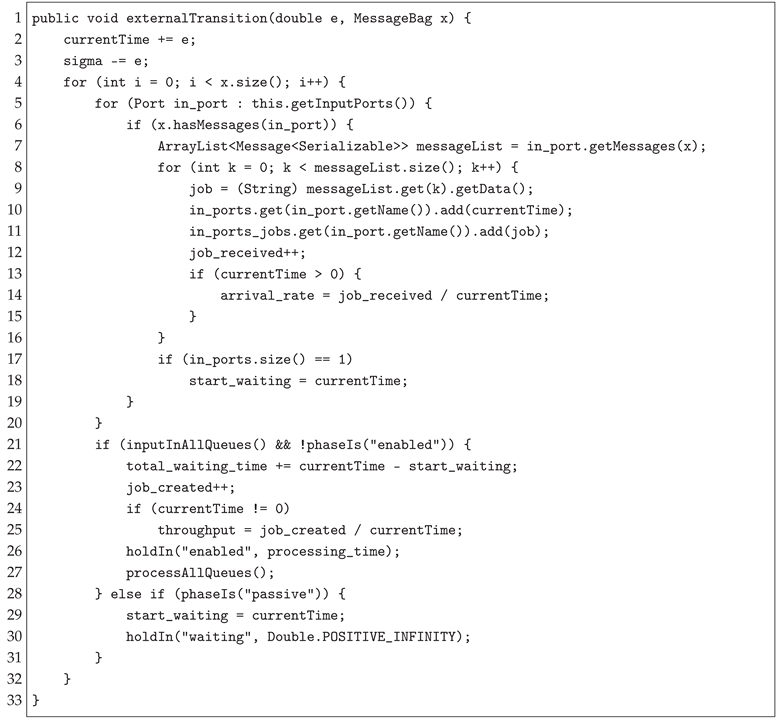 |
4. Experiments
We develop an exemplary model to illustrate the key aspects of the framework. Figure 3 shows the devised activity along with some sample simulation results. In this experiment, we observe staleness at the synchronizer via average queue size. The more the average size grows, the more staleness is observed. Since each stream feeds into the synchronization layer through a channel queue, the average size of the queues for the four incoming flows indicates the waiting time of inputs arriving through each of these flows.
The activity in Figure 3a illustrates four modalities each undergoing a latency stage () followed by stochastic jitter before entering the synchronizer. Modality encounters a delay specified by a uniform distribution , representing a lightweight latency. Modality encounters a delay specified as . Modality encounters a delay specified by an exponential distribution , followed by two parallel jitter models . Their outputs are merged afterward. Modality goes through a delay specified by a Gaussian distribution , representing higher latency. After this step, the flow undergoes a probabilistic branching. The input is forwarded to jitter with probability , and with probability , the input is dropped.
All jitter outputs are routed into the synchronizer block, which produces the combined output stream Y. All jitter models time advance function is specified with an exponential distribution .
We conducted four experimental setups to evaluate the effect of interarrival rate and dropping probability on the average waiting time within the synchronizer queues, thereby quantifying staleness by averaging through queue sizes. Each experiment is run over 10,000 time units. In the first setup, a new input is generated at every time unit and fed consecutively into one of the streams. In other words, an input is generated for each stream every 4 (i) time units. This produces the largest buildup of inputs in the synchronizer queues, since arrivals are frequent and often wait for higher-latency streams. The result is shown in Figure 3b, where staleness increases steadily. In the second setup, a new input is generated every 3 time units. As expected, the staleness is significantly smaller in Figure 3c. In the third setup, with inputs generated only every 5 time units, queue pressure is further reduced while showing some fluctuation in staleness, highlighting a typical dissipation behavior in queuing systems (Figure 3d).
In the fourth setup, the input rate is kept at every 5 time units, but the drop probability at the probabilistic branch of modality is increased to 25%. The goal is to introduce another source of pressure by increasing the dropping rate and then observing the staleness at the synchronizer. As expected, the results in Figure 3e show an increase in staleness due to the increased wait time of other, more frequent arrivals in faster streams.
Overall, the results of these four experiments validate the correctness of the simulation in two aspects. First, it confirms that higher input rates directly increase synchronizer queue occupancy. Second, increasing the dropping probability results in more waiting time for the incoming flow from other streams. These results highlight the trade-off between aspects of throughput and input pressure in synchronizing temporal multimodal streams.
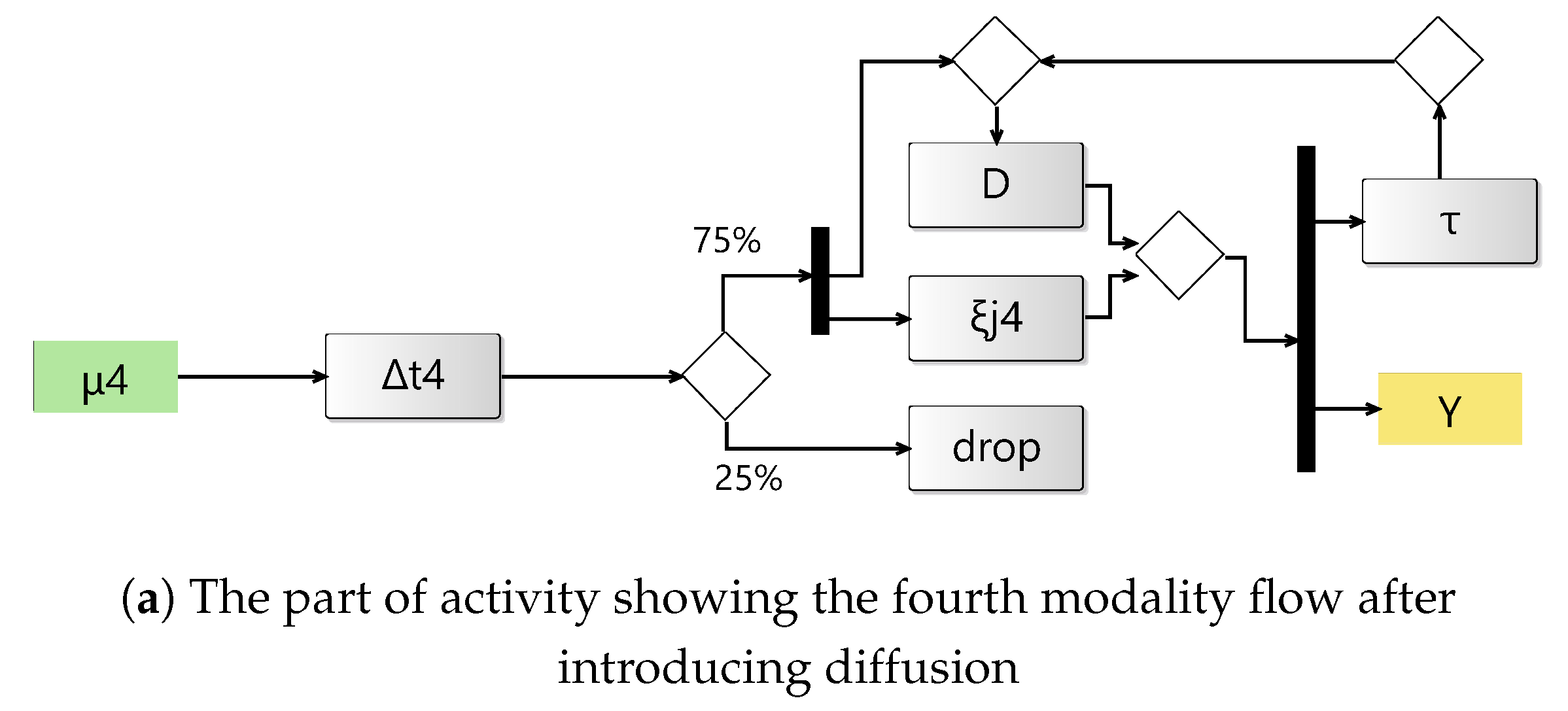
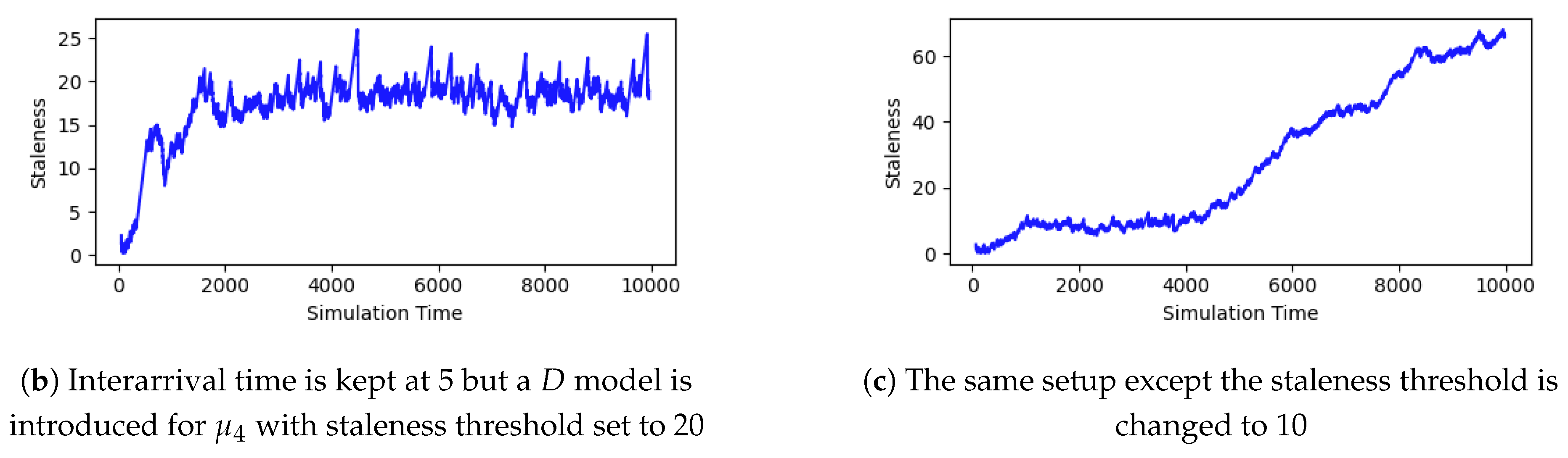
4.1. Event-Driven Restoration with Staleness Threshold
Now, we demonstrate the restoration of staleness levels in Figure 3d by introducing a diffusion model at the synchronizer. When the staleness level reaches a certain arbitrary threshold (e.g., 20), the synchronizer dispatches an output to the diffusion model to synthesize a replacement for the stream that is experiencing higher delays or a higher dropping rate. We run the experiment again with the same dropping rate (i.e., 25%) in . Our goal is to restore the same level of staleness as when the dropping rate was 5%. Thus, the diffusion model learns from previous inputs and is triggered when needed when the dropping rate increases. It can also be used as a tool to manipulate staleness and conduct further assessment and observation within the experimental frame. Figure 4a shows the part of the overall activity after adjusting for the diffusion model. Figure 4b shows the attempt to restore staleness in Figure 3d. In Figure 4c, we experiment by lowering the staleness threshold further (set to 10) to demonstrate the matching of multi-rate multimodal streams with temporal variability. The staleness stayed around 10 at the beginning of the simulation run. However, as the queues built up and started to accumulate from other flows, the upward trend began to increase steadily, and the effect of the threshold for diminished.
5. Discussion
This work aims to establish an M&S foundation to assess temporal multimodality. Our experiments highlight the complexity and sensitivity in modeling such streams. They also demonstrate the prospects as well as challenges that may arise due to the emergence of new modalities. By combining the inherent capabilities of AI models with a foundational simulation framework, we aim to deepen our understanding and, consequently, enhance the utilization of these capabilities to improve information streaming and communication at a broader scale.
The results in Section 4 demonstrate how variability in interarrival rates and dropping probabilities affects the overall model. By doing so, our goal is to validate the correctness of the simulation. Modelers can then modify the structure, add modalities, and calibrate the model to accurately represent various flow designs, thereby running and producing simulation results readily. We observed the input staleness to indicate the efficiency of synchronizing multiple incoming flows and to show the sensitivity of this metric to external factors in other model components. We tested the model with various synchronization policies for matching and ordering inputs. We note that we used a matching policy that combines incoming flows on a FIFO basis. However, the framework allows for the simulation of various policies, including timestamping, watermarking, event-driven, and multi-rate and latency synchronization.
We note the current limitations for integrating AI models, especially for high-speed streams. We are exploring more practical and computationally efficient ways to streamline AI models (i.e., diffusion) into the overall pipeline. Previous works address some underlying aspects of these limitations. Researchers have thoroughly discussed the problems of alignment among information streams [18], including jitter [19], dropping [20,21], expiration [22], among others. However, we point out that emergent enhancement requires a revisit to these issues and fostering innovative ways in light of the AI models’ native capacity.
In future work, we plan to conduct various experiments to further elaborate on these policies and how they can accommodate diffusion and upsampling enhancements to ensure the efficiency and reliability of the flow. We also plan to examine the potential enhancements of these models by increasing the interarrival and dropping rates, and reassessing the staleness and quality of the flow. We also plan to examine the validity of these metrics and apply them to autonomous decisions through sensor fusion.
6. Conclusions
Continuous assessment and calibration of multimodality in information streams can be a challenging endeavor. However, recent AI models have made significant advances, enabling more ways and removing some essential barriers to transformation in heterogeneous communication and information flows. In this paper, we tailor these models to address time-sensitive streams in a modular modeling & simulation environment. The flexibility offered by the modular DEVS Markov model enables the simulation of a wide range of possibilities in multimodal streaming, with a high degree of configurability and calibration of structural compositions and stochastic parameterization. Such support allows for a time-aware simulation of heterogeneous compositions of current and emerging modalities in information systems.
Funding
This research received no external funding.
Conflicts of Interest
The authors declare no conflict of interest.
Abbreviations
The following abbreviations are used in this manuscript:
| AI | Artificial Intelligence |
| DEVS | Discrete Event System Specification |
| FIFO | First In, First Out |
| M&S | Modeling & Simulation |
References
- Goodfellow, I.J.; Pouget-Abadie, J.; Mirza, M.; Xu, B.; Warde-Farley, D.; Ozair, S.; Courville, A.; Bengio, Y. Generative adversarial nets. Advances in neural information processing systems 2014, 27.
- Ho, J.; Jain, A.; Abbeel, P. Denoising diffusion probabilistic models. Advances in neural information processing systems 2020, 33, 6840–6851.
- Minaee, S.; Mikolov, T.; Nikzad, N.; Chenaghlu, M.; Socher, R.; Amatriain, X.; Gao, J. Large language models: A survey. arXiv preprint arXiv:2402.06196 2024. [CrossRef]
- Ramachandram, D.; Taylor, G.W. Deep multimodal learning: A survey on recent advances and trends. IEEE signal processing magazine 2017, 34, 96–108. [CrossRef]
- Xu, P.; Zhu, X.; Clifton, D.A. Multimodal learning with transformers: A survey. IEEE Transactions on Pattern Analysis and Machine Intelligence 2023, 45, 12113–12132. [CrossRef]
- Zeigler, B.P.; Muzy, A.; Kofman, E. Theory of modeling and simulation: discrete event & iterative system computational foundations; Academic press, 2018.
- Capocchi, L.; Zeigler, B.P.; Santucci, J.F. Simulation-Based Development of Internet of Cyber-Things Using DEVS. Computers 2025, 14, 258. [CrossRef]
- Zeigler, B. DEVS-based building blocks and architectural patterns for intelligent hybrid cyberphysical system design. Information 2021, 12, 531. [CrossRef]
- Seo, C.; Zeigler, B.P.; Kim, D. DEVS markov modeling and simulation: formal definition and implementation. In Proceedings of the Proceedings of the 4th ACM International Conference of Computing for Engineering and Sciences, 2018, pp. 1–12. [CrossRef]
- Jarraya, Y.; Debbabi, M.; Bentahar, J. On the meaning of SysML activity diagrams. In Proceedings of the 2009 16th Annual IEEE International Conference and Workshop on the Engineering of Computer Based Systems. IEEE, 2009, pp. 95–105. [CrossRef]
- Alshareef, A.; Sarjoughian, H.S. Hierarchical Activity-Based Models for Control Flows in Parallel Discrete Event System Specification Simulation Models. IEEE Access 2021, 9, 80970–80985. [CrossRef]
- Rozenblit, J.W. Experimental frame specification methodology for hierarchical simulation modeling. International Journal Of General System 1991, 19, 317–336. [CrossRef]
- Ptolemaeus, C., Ed. System Design, Modeling, and Simulation using Ptolemy II; Ptolemy.org, 2014.
- Sohl-Dickstein, J.; Weiss, E.; Maheswaranathan, N.; Ganguli, S. Deep unsupervised learning using nonequilibrium thermodynamics. In Proceedings of the International conference on machine learning. pmlr, 2015, pp. 2256–2265.
- Ao, S.; Hu, W.; Wang, S.; Li, B.; Yin, C.; Liu, X.; Zhang, J.; Song, X. Modeling and Simulation of Directed Graph-Based DEVS System. In Proceedings of the 2025 26th International Conference on Thermal, Mechanical and Multi-Physics Simulation and Experiments in Microelectronics and Microsystems (EuroSimE). IEEE, 2025, pp. 1–8. [CrossRef]
- MS4 Systems. MS4 Me Version 3.0. https://ms4systems.com/home, 2025. Accessed 9/1/2025.
- Hunter, J.D. Matplotlib: A 2D graphics environment. Computing in Science & Engineering 2007, 9, 90–95. [CrossRef]
- Kleinberg, J. Temporal dynamics of on-line information streams. In Data stream management: Processing high-speed data streams; Springer, 2016; pp. 221–238. [CrossRef]
- Hancock, J.; et al. Jitter—Understanding it, measuring it, eliminating it part 1: Jitter fundamentals. High Frequency Electronics 2004, 4, 44–50.
- Kirsch, C.M.; Payer, H.; Röck, H.; Sokolova, A. Performance, scalability, and semantics of concurrent FIFO queues. In Proceedings of the International Conference on Algorithms and Architectures for Parallel Processing. Springer, 2012, pp. 273–287. [CrossRef]
- Strzęciwilk, D. Timed petri nets for modeling and performance evaluation of a priority queueing system. Energies 2023, 16, 7690. [CrossRef]
- Golab, L.; Ozsu, M.T. Data stream management; Springer Nature, 2022. [CrossRef]
Figure 1.
Multi-layer architecture of handling temporal modality in streams.
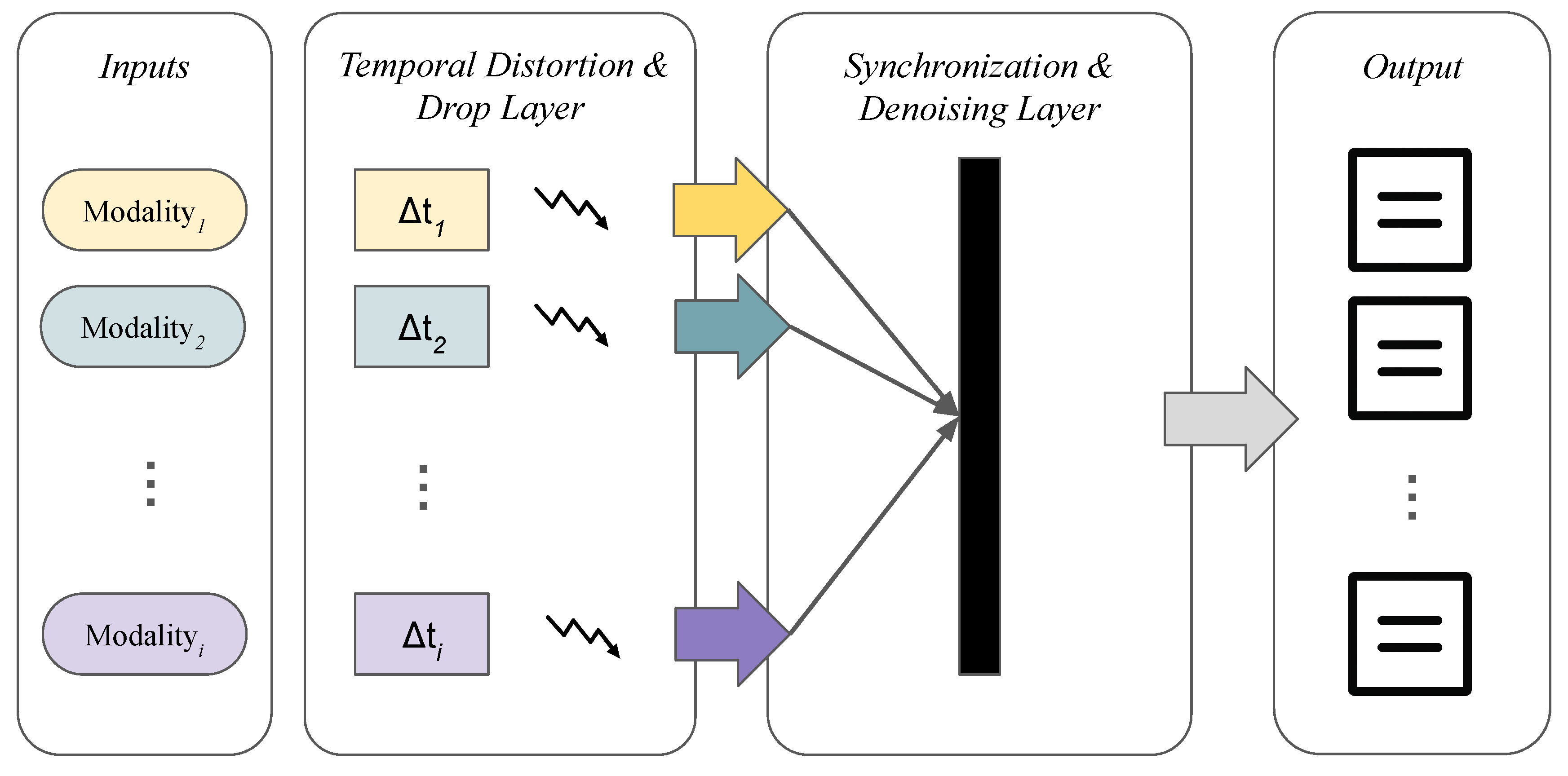
Figure 2.
A generic activity flow diagram for synchronizing multimodal streams.
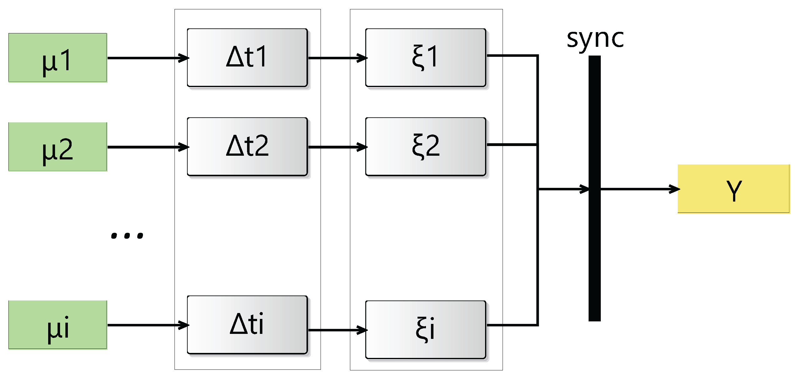
Figure 3.
The overall activity diagram and sample results after conducting four different experiment setups
Figure 3.
The overall activity diagram and sample results after conducting four different experiment setups
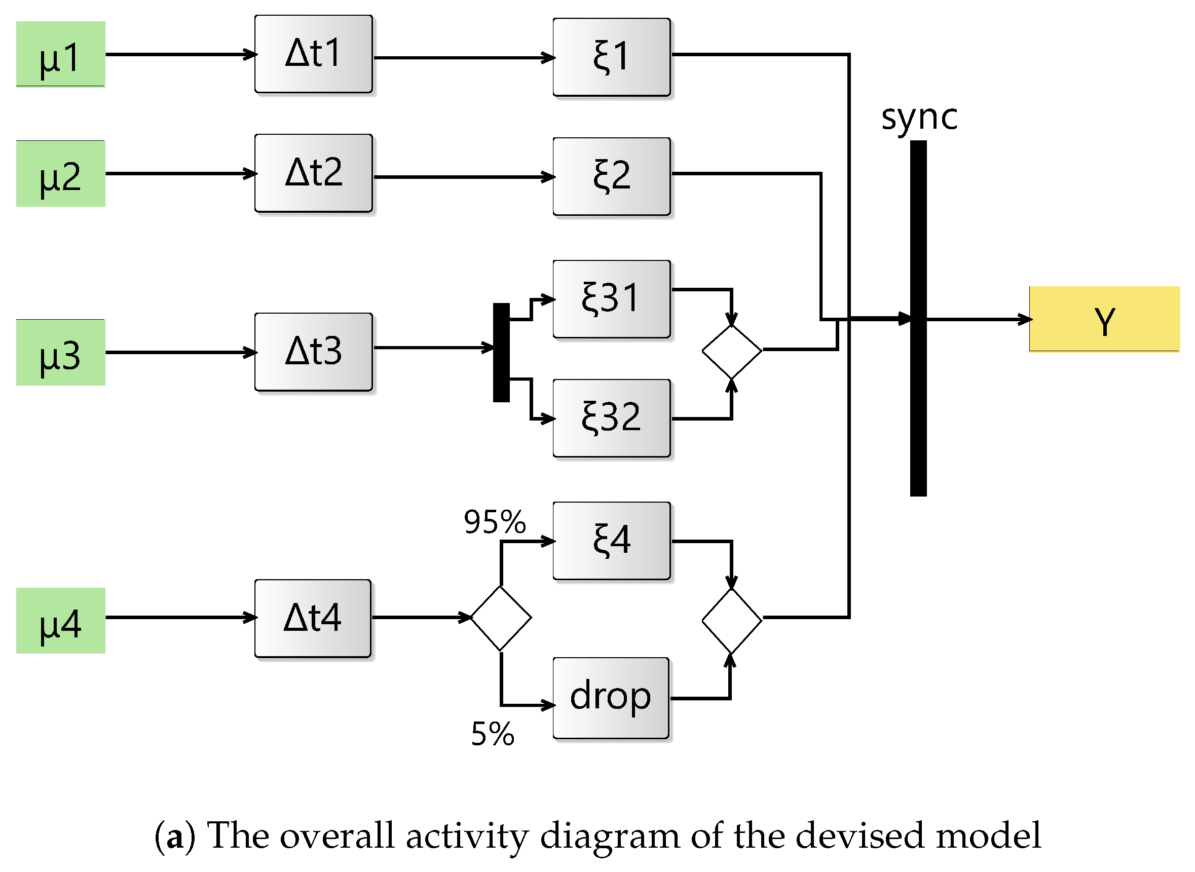
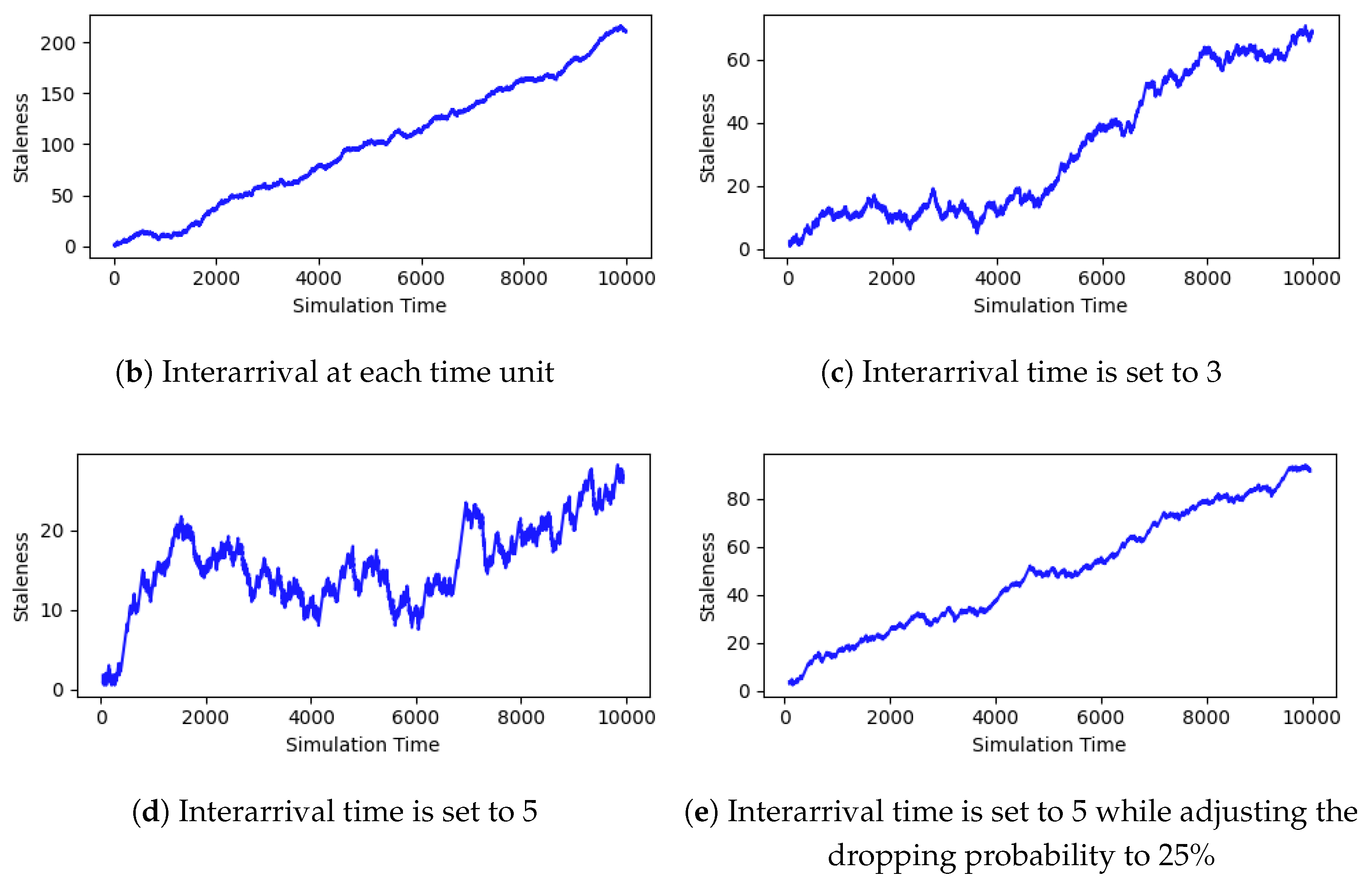
Figure 4.
The overall activity diagram and sample results after conducting four different experiment setups
Figure 4.
The overall activity diagram and sample results after conducting four different experiment setups
Disclaimer/Publisher’s Note: The statements, opinions and data contained in all publications are solely those of the individual author(s) and contributor(s) and not of MDPI and/or the editor(s). MDPI and/or the editor(s) disclaim responsibility for any injury to people or property resulting from any ideas, methods, instructions or products referred to in the content. |
© 2025 by the authors. Licensee MDPI, Basel, Switzerland. This article is an open access article distributed under the terms and conditions of the Creative Commons Attribution (CC BY) license (http://creativecommons.org/licenses/by/4.0/).
Copyright: This open access article is published under a Creative Commons CC BY 4.0 license, which permit the free download, distribution, and reuse, provided that the author and preprint are cited in any reuse.


