
Submitted:
30 September 2025
Posted:
01 October 2025
You are already at the latest version
Abstract
In a recent study \cite{isz00}, the authors derived exact black hole solutions in the framework of Einstein gravity coupled with a nonlinear electrodynamics field, considering additional matter sources in the form of a cloud of strings and a quintessence field. Building upon this foundation, we investigate the optical properties and dynamics of neutral test particles around spherically symmetric anti-de Sitter black holes in this scenario. The black hole solution is characterized by four key parameters: the mass $M$, the nonlinear charge parameter $k$, the cloud of strings parameter $\alpha$, and the quintessence field parameters $(\mathrm{N}, w)$. We analyze null geodesics using the Lagrangian formalism to examine photon trajectories, effective potential behavior, photon sphere formation, and shadow characteristics. The photon sphere radius and shadow size show systematic dependencies on all spacetime parameters, with shadow radii varying dramatically from $6.12$ to $19.30$ as the quintessence normalization changes. We calculate the Lyapunov exponent for circular null paths and examine photon trajectory formulations. For massive test particles, we examine effective potentials, innermost stable circular orbits, fundamental frequencies relevant to quasi-periodic oscillations, and periastron precession. The innermost stable circular orbit radius increases with cloud of strings and quintessence parameters while decreasing with the nonlinear charge parameter. Periastron precession analysis reveals radius-dependent frequency modulations with measurable deviations from standard general relativity. Our findings demonstrate how combined exotic matter sources significantly modify black hole spacetime geometry and orbital dynamics.
Keywords:
Black holes
; Nonlinear electrodynamics
; Cloud of strings
; Quintessence field
; Orbital dynamics
1. Introduction
Black holes (BHs) represent some of the most fascinating and extreme objects in the universe, serving as natural laboratories for testing the fundamental laws of physics under conditions of intense gravity. Among the various BH solutions in general relativity (GR), Anti-de Sitter (AdS) BHs have attracted considerable attention due to their rich geometric properties and profound connections to holographic duality [2,3,4]. AdS spacetimes are characterized by a negative cosmological constant (CC), leading to asymptotically AdS behavior that fundamentally alters the causal structure and thermodynamic properties compared to asymptotically flat spacetimes [5,6]. The AdS/CFT correspondence has established these geometries as crucial theoretical frameworks for understanding quantum gravity and strongly coupled field theories [7,8].
Cloud of strings (CoS) represents an exotic form of matter that has garnered significant interest in modified gravity theories and cosmological models. First introduced by Letelier [9], CoS configurations are characterized by a specific energy-momentum tensor that describes a spherically symmetric distribution of cosmic strings surrounding a central gravitating object. These configurations arise naturally in various theoretical contexts, including string theory compactifications and early universe cosmology [10,11]. The presence of CoS effectively weakens the gravitational field, leading to systematic modifications in horizon structure, geodesic dynamics, and observational signatures of BHs [12,13].
Quintessence fields (QF) constitute another crucial component in modern cosmology and modified gravity theories, representing a form of dark energy responsible for the observed accelerated expansion of the universe [14,15]. Unlike the cosmological constant, quintessence is characterized by a dynamic scalar field with an equation of state parameter w that can vary with time and space [16,17]. When quintessence surrounds BHs, it introduces power-law modifications to the metric function that depend critically on the equation of state parameter, leading to rich phenomenology in BH physics [18,19].
Nonlinear electrodynamics (NLED) represents a natural extension of Maxwell’s linear electromagnetic theory, incorporating field-dependent corrections that become significant in strong electromagnetic field regimes [20,21]. Born-Infeld theory, one of the most studied NLED models, was originally proposed to resolve the infinite self-energy problem of point charges and has found renewed interest in string theory and AdS/CFT contexts [22,23]. NLED modifications introduce exponential corrections to standard electromagnetic interactions, fundamentally altering the structure of charged BH solutions and their associated physical properties [24,25].
Quasi-periodic oscillations (QPOs) represent one of the most important observational signatures of matter dynamics around compact objects, providing direct insights into the strong-field gravitational regime [26,27]. These oscillations, observed in the X-ray light curves of accreting BH systems, are believed to originate from fundamental frequencies associated with particle motion in the vicinity of the innermost stable circular orbit (ISCO) [28,29]. The precise frequencies and their ratios carry crucial information about the BH parameters and the underlying spacetime geometry, making QPO observations powerful tools for testing theories of gravity [30,31,32].
Optical properties of BHs, including photon trajectories, shadow formation, and gravitational lensing effects, have emerged as premier observational windows into strong-field gravity [33,34]. The groundbreaking observations by the Event Horizon Telescope (EHT) of the shadows of M87* and Sagittarius A* have ushered in a new era of observational BH physics, enabling direct tests of GR predictions and constraints on alternative theories [35,36]. Photon dynamics around BHs is governed by effective potentials that encode information about spacetime geometry, providing signatures that can distinguish between different BH models and exotic matter configurations [37].
The motivation for this study stems from the recognition that realistic astrophysical BHs likely exist in environments containing multiple exotic matter sources, yet most theoretical investigations focus on simplified scenarios with single matter components. The latest progress in observational astronomy, especially in gravitational wave detection and electromagnetic imaging, necessitates more advanced theoretical models to explain the intricate matter distribution in actual astrophysical environments. Within AdS spacetimes, integrating CoS, QF, and NLED effects offers a notably comprehensive theoretical framework that highlights critical characteristics of modified gravity theories, yet remains manageable for in-depth study. Our primary aim is to provide a comprehensive investigation of the optical properties and particle dynamics around AdS BHs influenced by the combined presence of CoS, QF, and NLED effects. We seek to understand how these exotic matter sources collectively modify the fundamental properties of BH spacetimes, including horizon structure, photon sphere characteristics, shadow formation, and orbital dynamics of test particles. Through some analysis of null and timelike geodesics, we aim to identify observational signatures that could distinguish such exotic BH configurations from standard GR predictions. Specifically, we investigate how the four key parameters characterizing our BH solution - the mass M, NLED parameter k, CoS parameter , and QF parameters - influence the effective potentials governing photon and particle motion. We examine the formation and properties of photon spheres, analyze BH shadow characteristics with direct relevance to EHT observations, and determine the stability properties of circular orbits through Lyapunov exponent calculations. For massive test particles, we conduct detailed analysis of ISCO properties, effective radial forces, and fundamental frequencies relevant to QPO phenomena.
The paper is organized as follows: Section 2 presents the AdS BH geometry with CoS and QF in the NLED framework, examining the metric structure, horizon properties, and geometric characteristics. Section 3 analyzes the optical properties, including null geodesic dynamics, photon sphere formation, shadow characteristics, and topological features. Section 4 investigates the dynamics of neutral test particles, covering effective potentials, ISCO analysis, and fundamental frequencies. Section 5 summarizes our findings and discusses implications for observational astronomy and future theoretical developments.
2. AdS BH Geometry with CoS and QF in NLED Framework and Its Physical Characteristics
The geometric properties and horizon structure of BHs with CoS and QF in the NLED scenario provide fundamental insights into the spacetime structure of these gravitational systems. Building upon the foundational work by Letelier [9] on CoS-surrounded BHs and Kiselev [18] on QF-influenced spacetimes, we examine how the combined presence of these exotic matter sources affects the metric structure and causal properties in an AdS background.
The first study of a BH solution with a CoS as the source, within the framework of GR, was presented by Letelier [9]. In that work, he derived a generalization of the Schwarzschild BH surrounded by a spherically symmetric CoS, characterized by an energy-momentum tensor given by:
where is the energy density of the cloud and is an integration constant associated with the presence of the string. The Letelier BH solution is given by [9]
The study of the QF as a matter content within GR was carried out by Kiselev [18]. He obtained a generalization of the Schwarzschild solution describing a BH surrounded by a QF, with the corresponding energy-momentum tensor given by:
where denotes the energy density of the QF, and the pressure is related to the density via the equation of state , with being the quintessence state parameter. The corresponding line element is given by [18]:
Now, let us assume that the QF and the CoS do not interact with each other, allowing us to treat their combined energy-momentum tensor as a linear superposition of the individual contributions, given by:
Recent investigations into AdS black hole solutions featuring unconventional matter have illustrated the diverse geometric formations resulting from these setups [38,39,40]. The interaction between CoS and QF within AdS spacetimes causes alterations in metric functions, revealing the horizon structures [41,42,43].
A static and spherically symmetric AdS BH solution with a quintessence surrounded by a CoS in NLED is given by [1]
with the metric function is given by
Here is the cosmic strings parameter, M denotes the BH mass, represents the state parameter of quintessence matter, and N serves as quintessence positive normalization constant, is the non-linear self-gravitating magnetic charge, and is the CC. For a spherically symmetric space-time sourced only by a magnetic charge, the only non-null component of the electromagnetic field tensor is and the scalar is .
The geometric analysis of such gravitational systems requires careful examination of how each parameter influences the metric function and horizon formation. The metric function behavior shown in Figure 1 demonstrates the interplay between the various parameters. As observed in panel (a), increasing the CoS parameter leads to a systematic shift in the metric function, effectively modifying the spacetime geometry and horizon locations. The magnetic charge parameter k in panel (b) shows a more dramatic effect, particularly in the near-horizon region where NLED effects become dominant, introducing exponential modifications to the standard Schwarzschild form.
Noted that at large r, we have
Therefore, the metric function reduces as (since )
Thereby, one can recover a spherically symmetric RN-AdS BH metric with a CoS and quintessence.
The horizon structure analysis presented in Table 1 reveals the intricate relationship between the various parameters and the causal structure of the spacetime. The table systematically demonstrates how different parameter combinations lead to distinct BH configurations: extremal BHs with single horizons, non-extremal BHs with multiple horizons, or naked singularities where no horizons exist. For instance, when and , regardless of the CoS parameter , the system exhibits naked singularities. However, increasing the mass to with the same magnetic charge leads to non-extremal BH formation with two distinct horizons. This transition illustrates the critical role of the mass-to-charge ratio in determining the causal structure.
The embedding diagrams shown in Figure 2 provide a visual representation of how the spacetime geometry is modified by the presence of CoS, QF, and NLED effects. These diagrams illustrate the throat structure of the BH, where the red rings indicate the event horizon locations. Panel (a) shows the Schwarzschild-like AdS BH with QF, representing the baseline case with horizon at . Panel (b) demonstrates how moderate CoS strength () significantly enlarges the throat geometry, pushing the horizon outward to . Panel (c) reveals the combined effects of CoS and nonlinear magnetic charge, where the horizon moves even further to . Panel (d) shows the most dramatic geometric changes in the string-dominated regime with , where the horizon contracts to , indicating a highly modified spacetime structure.
The geometric implications of these modifications are significant for understanding the causal structure of the spacetime. The presence of CoS effectively modifies the gravitational potential, altering the location and number of horizons. The NLED effects introduce exponential corrections that become particularly important in the strong-field regime near the BH. The QF contribution depends critically on the equation of state parameter w, with values in the range characteristic of quintessence behavior that provides additional geometric modifications to the metric structure. The negative CC ensures the asymptotically AdS nature of the spacetime, providing a boundary condition that influences the global geometric properties.
In Figure 1, the metric function is plotted for the specific state parameter , showing its variation as a function of the radial distance r with different values of CoS parameter and magnetic charge k, while keeping all other parameters fixed.
3. Optical Properties of BH
In this work, we investigate the null geodesics around the chosen AdS BH and explore how different physical parameters influence the geodesic dynamics. Specifically, we examine the effects of the NLED parameter k, the CoS parameter , and the QF parameters . The motion of test particles is studied using the Lagrangian formalism [44,45,47,49,50,51,52,53], which provides a convenient and systematic way to derive the equations of motion.
To simplify the analysis, we restrict our attention to motion in the equatorial plane, defined by and , which is a valid assumption due to the spherical symmetry of the spacetime, where is an affine parameter. The standard form of the spacetime metric (6) is given by the following line element
where and denotes the metric tensor. This metric depends only on the radial coordinate r and the polar angle , and is independent of the time coordinate t and the azimuthal angle . As a result, the spacetime admits two Killing vector fields: and , which correspond to the invariance under time translations and rotations about the symmetry axis, respectively. According to Noether’s theorem, these symmetries give rise to two conserved quantities: the energy E associated with , and the angular momentum L associated with . These constants of motion play a crucial role in determining the trajectories of the test particles and allow us to reduce the geodesic equations to a more manageable form for both analytical and numerical analysis. In our case, we find these quantities
where is the conserved energy and is the conserved angular momentum.
The null geodesics is defined by and thereby, using spacetime (6), we find
Substituting Eq. (11) into Eq. (12) and after rearranging, we find
where the effective potential of the null geodesics is given by
The behavior of the effective potential shown in Figure 3 reveals the influence of the various parameters on photon trajectories. Panel (a) demonstrates how varying the CoS parameter systematically modifies the potential profile, with larger values leading to reduced potential magnitudes, effectively weakening the gravitational binding. The state parameter w also shows significant influence, with more negative values corresponding to stronger QF effects. Panel (b) illustrates the combined effects of CoS and NLED parameters, where the magnetic charge k introduces additional complexity in the potential structure. Panel (c) focuses on the interplay between CoS and QF effects, showing how these exotic matter sources collectively modify the photon dynamics around the BH.
The expression (14) shows that the effective potential for light-like particles is affected by several parameters. These include NLED represented by the parameter k, the CoS parameter , the QF parameters . Moreover, the potential is modified by angular momentum , the BH mass M and the CC . Together, these parameters modify the gravitational field of the BH, which in turn leads to modifications in the motion of light-like particles. The exponential term introduces NLED corrections that become particularly significant in the strong-field regime near the BH horizon, while the CoS parameter provides a constant offset that effectively reduces the gravitational strength. The QF term with its power-law dependence contributes additional long-range modifications that depend critically on the equation of state parameter w.
In Figure 3, behavior of the effective potential governs the dynamics of photons is plotted, showing its variation as a function of r with different values of the cloud of strings parameter , state parameter w, and magnetic charge k, while keeping all other parameters fixed.
Using the expression of the effective potential for null geodesics given in Eq. (14), one can recover some well-known results as follows:
These limiting cases demonstrate the generality of our framework and its ability to reproduce well-established results from the literature. The recovery of these known solutions provides confidence in our approach and establishes the proper connections to previous work in the field of BH physics with exotic matter sources.
3.1. Effective Radial Force Experiences by Photons
In this subsection, we investigate how the dynamics of photon particles are affected by the gravitational field generated by NLED, CoS, and a QF, which together act as the sources of the BH spacetime. The force acting on photon particles can be analyzed using the effective potential for null geodesics, as given in Eq. (14). This force in terms of effective potential is defined by
where we have used Eq. (14).
The radial force behavior illustrated in Figure 4 demonstrates the influence of the various spacetime parameters on photon dynamics. Panel (a) shows how the magnetic charge parameter k significantly affects the force profile, with larger values leading to more pronounced variations in the force magnitude, particularly in the intermediate radial regions. Panel (b) reveals the systematic effect of the CoS parameter , where increasing values generally reduce the magnitude of the attractive force, consistent with the weakening of gravitational effects due to the presence of the string cloud. The force profiles exhibit characteristic features including regions of attraction (negative force) and potential repulsion (positive force), which are crucial for understanding photon capture and escape dynamics.
The above expression (20) shows that the force on photon particles is affected by several parameters involved in the BH spacetime. These include the NLED source represented by the parameter k, the CoS parameter , the QF parameters . Moreover, the force is also modified by the angular momentum and BH mass M. Together, these parameters modify the dynamics of photon particles in the given gravitational field of the BH solution. The exponential terms involving k introduce NLED corrections that become particularly significant in the strong-field regime, while the CoS parameter provides a constant offset that systematically reduces the gravitational attraction. The QF contribution depends on the power-law term that varies with the equation of state parameter w.
For a specific state parameter, for example, , the force on photon particles from Eq. (20) is given by
In Figure 4, behavior of the effective radial force experiences by photon particles is plotted for the specific state parameter , showing its variation as a function of the radial distance r with different values of CoS parameter and magnetic charge k, while keeping all other parameters fixed.
Using the above expression of force on photon particles, one can recover some well-known results:
These limiting cases provide important consistency checks and demonstrate how our general framework encompasses various well-studied scenarios in the literature. The systematic recovery of these known results validates our approach and establishes the proper connections between different models of BH physics with exotic matter sources.
3.2. Photon Sphere, BH Shadow and Lyapunov Exponent
In this subsection, we explore the influence of NLED, CoS, and a QF-considered as combined sources shaping the gravitational field of the BH spacetime-on key aspects of photon dynamics. Specifically, we examine how these factors affect the photon sphere radius, the properties and stability of circular null orbits, and the overall behavior of photon trajectories in the curved spacetime.
For circular null geodesics, the conditions and must be satisfied, leading to the following two relations:
where prime denotes partial derivative w.r.t. r.
The first relation in Eq. (26) gives us the critical impact parameter for photons. Moreover, the relation gives us the photon sphere radius satisfying the following equation
The expression given in Eq. (27) shows that the radius of the photon sphere is influenced by the NLED source parameter k, the CoS parameter , the QF parameters , and the BH mass M. Together, these factors modify the size of the photon sphere in the given gravitational field.
For a specific state parameter, for example, , the photon sphere radius is given by
The three-dimensional visualization of the photon sphere radius shown in Figure 5 reveals the parameter dependencies of this critical orbital radius. Panel (a) demonstrates how the photon sphere radius varies with both the CoS parameter and the QF normalization . The surface shows a systematic increase in with increasing , indicating that the presence of CoS effectively enlarges the photon sphere by weakening the gravitational field. Panel (b) illustrates the combined effects of CoS and NLED parameters, where the magnetic charge k tends to reduce the photon sphere radius, counteracting the enlarging effect of the CoS. These 3D surfaces provide intuitive understanding of the parameter space and guide the selection of physically relevant values for detailed analysis.
The expression given in Eq. (28) shows that the radius of the photon sphere is influenced by the NLED source parameter k, the CoS parameter and the QF normalization constant . Together, these factors modify the size of the photon sphere in the given gravitational field. Obtaining an analytical solution for Eq. (28) is challenging due to the transcendental nature of the exponential terms. Consequently, we determine the photon sphere radius numerically by selecting suitable values for the geometric and physical parameters , k and .
We proceed to compute the shadow radius of the BH and examine the effects of the spacetime’s geometrical parameters on its size. The BH shadow is an observable feature defined as the dark, lensed image of the event horizon against an emitting background. This effect occurs due to the high deflection of light rays in the strong-field gravity regime, with the shadow’s boundary originating from photons on unstable circular orbits at the photon sphere radius . The measurable shadow radius is geometrically linked to the critical impact parameter for photon capture. In the case of a static, spherically symmetric BH, is given by the following relation:
Using Eq. (26), we find the following expression for shadow radius
Correspondingly, the angular radius of the shadow observed at a distance D from the BH is given by:
The shadow radius behavior illustrated in Figure 6 demonstrates the systematic influence of the various spacetime parameters on the observable shadow size. Panel (a) shows how the shadow radius increases with both the CoS parameter and the QF normalization , with the effect being more pronounced for larger values of these parameters. Panel (b) reveals the competing effects between CoS and NLED parameters, where increasing k tends to reduce the shadow size while increasing enlarges it. These trends are crucial for understanding observational signatures and constraining model parameters through shadow measurements.
In Table 2, we present numerical values of the photon sphere radius as well as the shadow size by varying the string parameter , magnetic charge k and QF normalization . The data systematically demonstrates several important trends: increasing leads to larger photon sphere radii and shadow sizes, reflecting the weakening gravitational effects due to CoS. Conversely, increasing the magnetic charge k generally reduces both quantities, indicating the strengthening effects of NLED. The QF parameter shows the most dramatic effect, with shadow radius increasing from to as varies from to . These dependencies are crucial for interpreting observations such as those made by the EHT, which aims to constrain the properties of BHs through shadow imaging [35].
Figure 5 depict the photon sphere radius for the specific state parameter , showing its variation as a function of and , while keeping all other parameters fixed.
Figure 6 depict the shadow radius for the specific state parameter , showing its variation as a function of and , while keeping all other parameters fixed.
Figure 7 displays the BH shadow rings for various values of the NLED parameter k, the CoS parameter and QF constant . For a fixed k and , the shadow size increases with , as the CoS reduces the BH’s gravitational pull, enlarging the photon sphere. The left panel shows concentric circles with increasing radii as increases from to . Conversely, for a fixed and , the shadow size decreases with increasing k, a result of the photon’s coupling to the NLED field. The middle panel demonstrates this trend with decreasing shadow sizes as k increases. Finally, for fixed k and , the shadow size increases dramatically with , as shown in the right panel where the outermost circle corresponds to , illustrating the influence of QF on the observable shadow properties.
3.3. Unstable Circular Null Orbits: Lyapunov Exponent
We now turn our attention to the stability of circular null geodesics at the radius , analyzing how NLED, CoS, and a QF influence this stability. The Lyapunov exponent, as defined in [56], provides a useful tool for determining the stability of circular orbits and is given by:
where and is the effective potential for null geodesics.
With the help of effective potential given in Eq. (14), we find
where we have used the relation for circular null geodesics.
Substituting Eq. (33) into Eq. (32) and finally using from Eq. (26), we find the Lyapunov exponent given by
The expression (34) shows that the Lyapunov exponent for circular null geodesics is influenced by several parameters. These include the NLED parameter k, the CoS parameter , the QF parameters , and the BH mass M including the CC . The Lyapunov exponent provides crucial information about the stability of photon orbits at the photon sphere. Positive real values indicate unstable orbits where small perturbations grow exponentially, while the magnitude determines the timescale for this instability. The intricate interaction among parameters results in sophisticated stability structures, highly sensitive to spacetime parameter values.
For a specific state parameter, for example, , we find from Eq. (34)
In Figure 8, behavior of the Lyapunov exponent is plotted for the specific state parameter , showing its variation as a function of the radius of the circular null orbits with different values of CoS parameter and magnetic charge k, while keeping all other parameters fixed. We have observed that the Lyapunov exponent remains positive, indicating unstable circular null orbits.
Using the above expression (34) of the Lyapunov exponent, one can recover some well-known results:
Now, we define the geodesic angular velocity (coordinate) as follows:
where we have used the relation (26).
Substituting the metric function from Eq. (7), we find the geodesic angular velocity given by
The expression (41) shows that the geodesic angular velocity for circular orbits is affected by the NLED represented by the parameter k, the CoS parameter , the QF parameters , the BH mass M, and the CC . The angular velocity provides important information about the orbital dynamiCoS at the photon sphere and is directly related to the observable properties of the system.
For a specific state parameter, for example, , we find from Eq. (41)
The Lyapunov exponent and angular velocity together provide a complete characterization of the stability and dynamical properties of circular photon orbits in this gravitational environment. These quantities are essential for understanding the astrophysical signatures of such exotic BH configurations and their potential detectability through future gravitational wave observations and electromagnetic imaging.
3.4. Photon Trajectory Equation
In this part, we focus on the photon trajectory and show how light bends in the given gravitational field and examine the effects of the NLED parameter k, the CoS parameter , the QF parameters , and the CC .
Transforming to a new variable via into Eq. (43) and after simplification, we find
Equation (44) represents the photon trajectory in the given gravitational field produced by the BH solution. We observe that the photon trajectory is influenced by the NLED parameter k, the CoS parameter , the QF parameters , and the BH mass M including the CC . The first-order differential equation shows how the various exotic matter sources contribute to the orbital dynamics through different functional dependencies on the inverse radial coordinate u.
To derive a second-order differential equation for photon trajectory, we differentiate Eq. (44) w.r.t. and after simplification, we find
The above photon trajectory equation (45) fundamentally depends on the NLED parameter k, the CoS parameter , the QF parameters , and the BH mass M. Notably, the second-order differential equation for photon trajectory becomes independent of both the impact parameter and the CC , indicating that these quantities affect the initial conditions and boundary behavior but not the local curvature effects that determine the bending dynamics.
For a specific state parameter, for example, , we find from Eq. (45) the second-order differential equation for photon trajectory as:
This trajectory equation reveals the interplay between the various spacetime modifications. The CoS parameter appears as a modification to the effective "frequency" of the harmonic oscillator-like term, reducing the restoring force when . The NLED contribution through the exponential term introduces highly nonlinear effects that become significant at small radii (large u). The QF provides a constant driving term for this specific equation of state, which can significantly alter the photon trajectories, particularly for bound or nearly bound orbits.
The mathematical structure of Eq. (46) represents a modified harmonic oscillator with exponential and constant forcing terms, whose solutions describe the photon trajectories in this exotic gravitational environment. These trajectories are essential for understanding light deflection, gravitational lensing effects, and the formation of photon rings around such BHs [57].
3.5. Topological Features of Photon Sphere
Topological methods have recently become powerful tools for analyzing BH solutions. In particular, Duan’s -mapping theory connects topological defects-arising where vector fields vanish-with critical points and phase transitions in BH systems. These defects generate a conserved topological current, leading to a topological invariant that encodes the system’s global phase structure through geometric properties of the vector field. For comprehensive studies and applications in various BH contexts, see [58,59,60,61,62,63,64,65,66].
In order to study the topological property of the PR, one can introduce a potential function as follows [58,59,60,62]:
The behavior of the potential function shown in Figure 9 reveals the characteristic features that determine the photon sphere location and its topological properties. Panel (a) demonstrates how varying the CoS parameter and the QF state parameter w affects the potential profile. The curves show distinct minima that correspond to the photon sphere radii, with the position and depth of these minima being sensitive to the parameter values. Panel (b) illustrates the combined effects of CoS and NLED parameters, where the magnetic charge k introduces additional structure in the potential. Panel (c) focuses on the interplay between CoS and QF effects, showing how these exotic matter sources collectively modify the potential landscape that governs photon dynamics.
Obviously, the radius of the photon sphere locates at the root of . Similar to [58,59,60,62], we can introduce a vector :
It follows that . Although the circular photon orbit for a spherically symmetric BH is a photon sphere, which is independent of the coordinate , here we aim to investigate the topological property of the circular photon orbit, so we preserve in our discussions. Note that the vector field can also be reformulated as
The normalized vectors are defined as
The vector field visualizations presented in Figure 10, Figure 11, and Figure 12 provide insight into the topological structure of the photon sphere in this gravitational environment. Figure 10 shows how the CoS parameter affects the vector field orientation and magnitude across the plane. As increases from to , the vector field patterns show systematic changes that reflect the modification of the underlying spacetime geometry. Figure 11 demonstrates the influence of the NLED parameter k, where increasing magnetic charge values lead to more complex vector field structures, particularly in regions close to the photon sphere. Figure 12 illustrates the effect of the QF normalization parameter , showing how quintessence modifications alter the topological properties of the system.
In our case, we find the vector field components and as:
Here represents the standard point at which the vector field vanishes. Note that at and , both components vanish.
The magnitude of the vector field is given by
Thereby, the normalized vector field components are:
From the above expressions (54)–(55), we observe that the normalized vector is modified by the CoS parameter , the normalization of the QF, and the NLED parameter k. Moreover, the BH mass M and CC also alter these topological characteristics. The topological analysis provides a framework to the geometric analysis, revealing how the exotic matter sources influence not only the local dynamics but also the global topological structure of the photon sphere region.
By comparing the current results of the normalized vector field components given in Eqs. (56)–(57) with those presented in Eqs. (58)–(65), we observe that the string parameter , the nonlinear electrodynamics (NLED) parameter k, and the normalization constant associated with the quintessence-like field collectively modify the structure of the normalized vector field and lead to noticeable shifts in the results.
4. Dynamics of Neutral Test Particles
In this section, we analyze the dynamics of neutral test particles in the gravitational field of the selected BH spacetime. Of particular interest is the behavior of particles in circular motion, especially the characteristics of the ISCO, which play a crucial role in understanding accretion processes and astrophysical observations. We also examine the effective radial force acting on these particles, which determines the nature of their trajectories and stability.
The Hamiltonian describing the motion of a neutral particle is expressed by [67,68,69,70]
where is the mass of the neutral particle, is the four-momentum, is the four-velocity, and is the proper time of the neutral particle. The Hamilton equations of motion are given by:
and
where the affine parameter is given by .
Using the normalization condition and the metric (6), we find
Since the metric components are independent of the temporal coordinate t and the azimuthal coordinate , the corresponding components of the particle’s four-momentum, namely and , are conserved along its geodesic trajectory. These quantities represent the conserved energy and angular momentum of the particle, respectively:
where and are the specific energy and angular momentum per unit mass of the neutral particle, respectively. Moreover, the conjugate momentum associated with the coordinate is given by
The four-velocity components of timelike particles, including the temporal (), azimuthal () and radial () components, obey the following equations of motion:
where the four-velocity satisfies the timelike condition .
The effective potential behavior for neutral test particles shown in Figure 13 reveals the influence of the various spacetime parameters on massive particle dynamics. Panel (a) demonstrates how the CoS parameter and QF state parameter w systematically modify the potential wells that govern bound orbits. The potential profiles show characteristic minima that correspond to stable circular orbits, with the depth and location of these minima being sensitive to the exotic matter parameters. Panel (b) illustrates the combined effects of CoS and NLED parameters, where the magnetic charge k introduces additional structure in the potential landscape. Panel (c) focuses on the interplay between CoS and QF effects, showing how these matter sources collectively alter the orbital dynamics around the BH.
4.1. Effective Potential and Circular Motion
The Hamiltonian H can be expressed as
Using Eqs. (70)–(71), we can re-write the above Hamiltonian as:
where is the effective potential of the system and is given by
The expression (78) shows that the effective potential governing the dynamics of neutral test particles is influenced by several geometric and physical parameters. These include NLED represented by the parameter k, the CoS parameter , the QF parameters . Moreover, the potential is modified by angular momentum , the BH mass M and the CC . Together, these parameters modify the gravitational field of the BH, which in turn leads to modifications in the motion of massive particles. The effective potential determines the allowed regions of motion, the existence of bound orbits, and the stability properties of circular trajectories.
For circular motion, the conditions and must be satisfied. These conditions imply the following two relations:
where prime denotes ordinary derivative w.r.t. r.
The specific angular momentum behavior illustrated in Figure 14 demonstrates how the various spacetime parameters affect the orbital characteristics of neutral test particles. Panel (a) shows the systematic variation of with radial coordinate for different values of the magnetic charge parameter k. The curves exhibit characteristic increases with radius, reflecting the centrifugal barrier effects, with NLED modifications introducing subtle but measurable changes in the angular momentum requirements for circular orbits. Panel (b) reveals the influence of the CoS parameter , where larger values systematically increase the angular momentum needed for stable circular motion at any given radius, consistent with the weakening gravitational effects due to the string cloud.
The specific energy profiles shown in Figure 15 complement the angular momentum analysis by revealing the energy requirements for circular orbits in this gravitational environment. Panel (a) demonstrates how the NLED parameter k affects the binding energy of circular orbits, with larger magnetic charge values generally requiring higher energies for stable motion. Panel (b) shows the systematic effect of the CoS parameter , where increasing string strength leads to reduced binding energies, reflecting the overall weakening of the gravitational potential. These energy curves are essential for understanding the energetics of accretion processes and the formation of accretion disks around such exotic BHs.
From expressions (81)-(82), it becomes evident that the specific angular momentum and the specific energy associated with neutral test particles are influenced by several geometric and physical parameters. These include NLED represented by the parameter k, the CoS parameter , the QF parameters . Moreover, the BH mass M and the CC also influence these physical quantities.
4.2. Determining the Innermost Stable Circular Orbits
The minimum and maximum values of the effective potential correspond to stable and unstable circular orbits, respectively. In Newtonian gravity, the ISCO does not have a minimum bound on the radius; the effective potential always exhibits a minimum for any given angular momentum. However, this behavior changes when the effective potential depends not only on the angular momentum of the particle but also on additional factors, such as spacetime curvature or external fields.
In GR, the effective potential for particles orbiting near a Schwarzschild BH features two extrema-one minimum and one maximum-for a given angular momentum. At , where is the Schwarzschild radius, these two extrema coincide at a critical value of angular momentum, marking the location of the ISCO. This point defines the transition from stable to unstable circular orbits. The ISCO can be determined by applying the following conditions to the effective potential :
Using the effective potential expression given in Eq. (78), we find the following relation:
Using the metric function, we find the following polynomial relation in r as:
For a particular state parameter, , we find:
The three-dimensional visualization of the ISCO radius shown in Figure 16 provides insight into how the combined effects of CoS and NLED parameters influence this critical orbital radius. The surface demonstrates that increasing the CoS parameter generally leads to larger ISCO radii, reflecting the weakening gravitational effects due to the string cloud. Conversely, increasing the magnetic charge parameter k tends to reduce the ISCO radius, indicating the strengthening gravitational effects due to NLED modifications. The topology of this surface reveals regions where these competing effects balance, creating intricate parameter dependencies that are crucial for understanding accretion disk formation and stability in such exotic gravitational environments.
Equation (88) is a polynomial relation in r of infinite degree whose exact analytical solution is quite challenging. However, one can determine numerical values of ISCO radius by setting suitable values of parameters (see Table 4). The numerical data systematically demonstrates several important trends: increasing leads to larger ISCO radii, with values ranging from to as varies from to . The magnetic charge parameter k shows the opposite trend, with ISCO radii decreasing from to as k increases from to . The QF parameter exhibits the most dramatic effect, with ISCO radii increasing from to as varies from to . Thereby, it becomes evident that the ISCO radius is influenced by the magnetic charge parameter k, CS parameter , the QF parameters . Moreover, the BH mass M and the CC also influence this radius.
Modifications to the ISCO possess noteworthy ramifications for the physics of accretion in the vicinity of such exotic black holes. Systematic changes in the ISCO radius exert a direct impact on the inner boundary of accretion disks, thereby affecting the efficiency of energy extraction, the spectral characteristics of emitted radiation, and the dynamics of matter descending into the black hole. Comprehending these interdependencies is essential for the interpretation of observational data from astrophysical black holes and for constraining the parameters of exotic matter models through astronomical observations [71].
4.3. Effective Radial Force
The effective radial force experienced by the neutral test particles can be determined using the effective potential which governs the dynamics of neutral test particles in the gravitational field. This force is the negative gradient of the potential given by
Substituting the potential (78), we find the following expression:
The radial force behavior illustrated in Figure 17 demonstrates the influence of the various spacetime parameters on the dynamics of neutral test particles. Panel (a) shows how the magnetic charge parameter k affects the force profile, with larger values introducing more oscillatory behavior in the force, particularly in the intermediate radial regions where NLED effects compete with gravitational attraction. Panel (b) reveals the systematic effect of the CoS parameter , where increasing values generally reduce the magnitude of the attractive force, consistent with the weakening gravitational effects due to the string cloud. The force profiles exhibit regions of both attraction (negative force) and repulsion (positive force), which are crucial for understanding particle confinement and escape dynamics in these exotic gravitational environments.
From expression (90), it becomes evident that the effective radial force experienced by the neutral test particles is influenced by the magnetic charge k, CoS parameter , the QF parameters . Moreover, the BH mass M and the CC also influence these physical quantities. The first term in the expression represents the direct gravitational and exotic matter contributions, while the second term encodes the centrifugal effects modified by the various spacetime parameters.
4.4. Fundamental Frequencies
To analyze the oscillatory behavior of massive test particles, we consider small perturbations around SCO. When such a particle is slightly displaced from its equilibrium position within the equatorial plane, it exhibits EM, which can be effectively modeled as linear HO. This framework provides a powerful tool for examining the oscillation frequencies and assessing the stability characteristics of the particle’s trajectory in a given spacetime geometry. Several studies have employed this method in various gravitational contexts to gain insights into particle dynamics and stability criteria [71,72,73,74,75].
I. Local Frequencies
The frequencies as measured by a local observer in circular orbits of radius r are given by:
Using the given potential in Eq. (78), we find these frequencies in terms of the metric function at radius and as follows:
where is given by
II. Distant Observer Frequencies
The Keplerian frequency, , is a fundamental frequency associated with the orbital motion of a test particle around a central massive object. The Keplerian frequency is given by:
Azimuthal frequency , which is the frequency of Keplerian orbits of test particles in the azimuthal direction, is given by:
The radial and vertical angular frequencies and are the frequencies of oscillations of the neutral test particles in the radial direction along the stable orbits, which can be determined from the second derivatives of the effective potential by r and coordinates, respectively:
The frequency analysis reveals the characteristic oscillation behavior of neutral test particles in the exotic gravitational environment created by the combined presence of CoS, QF, and NLED effects. These frequencies are directly observable through QPO phenomena in astrophysical systems and provide crucial constraints on the underlying spacetime parameters. Figure 18 demonstrates the radial frequency behavior as a function of orbital radius . Panel (a) shows how varying the CoS parameter from 0.05 to 0.30 systematically modifies the radial oscillation frequencies, with larger values generally leading to reduced frequencies due to the gravitational weakening effect of the string cloud. The curves exhibit characteristic maxima that shift to larger radii as increases, indicating that the most efficient radial oscillations occur at progressively larger orbital distances in string-dominated environments. Panel (b) illustrates the influence of the NLED parameter k, where increasing magnetic charge values from 0.1 to 0.4 introduce more complex frequency structures. Figure 19 presents the vertical angular frequency variations with orbital radius. Both panels show monotonically increasing frequency profiles, reflecting the strengthening of vertical restoring forces at larger radii due to the gravitational field geometry. Panel (a) demonstrates that increasing systematically reduces the vertical oscillation frequencies across all radii, consistent with the overall weakening of gravitational binding due to CoS effects. Panel (b) reveals that NLED modifications through the parameter k introduce more subtle but measurable changes in the vertical frequency structure, with larger magnetic charges generally leading to enhanced vertical oscillations at intermediate radii. Figure 20 displays the azimuthal frequency behavior, which corresponds directly to the Keplerian orbital frequency and represents the most readily observable frequency in astrophysical systems. Panel (a) shows how the QF state parameter w influences the orbital frequency, with more negative values (stronger quintessence effects) leading to systematically lower frequencies due to the additional gravitational modifications introduced by the scalar field. The frequency profiles exhibit the expected scaling characteristic of Keplerian motion, but with systematic deviations that encode information about the exotic matter parameters. Panel (b) demonstrates the NLED effects on orbital frequencies, where increasing k values produce measurable frequency shifts that could be detected through high-precision timing observations of orbiting matter. These frequency modifications have direct implications for QPO observations in BH systems.
Overall, these parameter dependencies provide a theoretical framework for interpreting observed frequency ratios and their evolution, potentially enabling constraints on exotic matter models through comparison with observational data from X-ray timing studies of accreting BHs. The frequency relationships could also determine the characteristic timescales for accretion disk instabilities and emission variability patterns.
4.5. Periastron Precession
Periastron precession represents a fundamental relativistic phenomenon where the closest approach point (periastron) of a bound orbital trajectory advances progressively with each orbital period. This effect provides crucial observational signatures for testing GR and constraining exotic matter models through precision astrometry of stellar orbits around compact objects [76,77].
In the context of our AdS BH spacetime with CoS, QF, and NLED effects, periastron precession arises from the non-Keplerian modifications to the gravitational potential. The precession rate can be calculated from the fundamental orbital frequencies governing small perturbations around circular orbits.
The periastron precession frequency is defined as the difference between the azimuthal orbital frequency and the radial epicyclic frequency [78,79,80]:
where represents the mean orbital frequency and characterizes the radial oscillation frequency.
From our previous analysis in Section 4, these frequencies are expressed directly in terms of the metric function as:
The complete expression for the periastron precession frequency becomes:
Substituting these expressions into Eq. (105) provides the complete precession frequency in terms of the metric function and all spacetime parameters . The precession rate exhibits remarkable dependencies on all spacetime parameters. The CoS parameter reduces the precession rate by weakening the overall gravitational field strength, effectively diminishing the relativistic corrections that drive orbital advance. The NLED parameter k introduces exponential corrections that become particularly significant in the strong-field regime near the BH, where the nonlinear electromagnetic effects can either enhance or suppress the precession depending on the orbital radius and magnetic field configuration. The QF parameters contribute power-law modifications that predominantly affect the precession at larger radii, with the quintessence field providing additional gravitational modifications that systematically alter the orbital dynamics. Finally, the negative CC provides additional corrections to the precession rate through its influence on the asymptotic spacetime geometry, creating long-range modifications that distinguish AdS spacetimes from their asymptotically flat counterparts.
The precession angle per orbit can be calculated as:
This expression provides direct observational predictions that can be compared with astrometric measurements of stellar orbits around BHs. The systematic parameter dependencies enable constraints on exotic matter models through precision measurements of orbital precession rates. The modifications introduced by the exotic matter sources create measurable deviations from the classical GR prediction of for Schwarzschild spacetime, with the deviations encoding information about the underlying spacetime parameters.
The periastron precession in this exotic gravitational environment differs significantly from standard GR predictions, with the combined effects of CoS, QF, and NLED creating measurable deviations that could distinguish such BH models from conventional scenarios through future high-precision astrometric observations. The exponential NLED corrections become particularly important in the strong-field regime, while the power-law QF modifications dominate at larger radii, providing complementary observational windows for constraining exotic matter parameters.
Figure 21 and Figure 22 show the periastron precession frequency in the equatorial plane, highlighting how the exotic matter sources modify the classical precession pattern through systematic parameter variations. Figure 21 demonstrates the precession frequency behavior for a strongly negative CC (), where the AdS curvature effects are pronounced. The curves exhibit characteristic U-shaped profiles with minima corresponding to stable circular orbits, with the minimum precession frequency decreasing as the CoS parameter increases from 0.05 to 0.20. For instance, panel (a) shows that at , the minimum precession frequency occurs around , while increasing magnetic charge k (indicated by the color gradient from blue to red) systematically shifts the curves, with higher k values generally reducing the precession frequency at small radii due to enhanced NLED effects. As increases to 0.20 in panel (d), the minimum shifts to larger radii (), reflecting the weakening gravitational pull due to the string cloud. Figure 22 presents analogous behavior for a weaker CC (), where the reduced AdS curvature allows precession to persist at larger orbital radii. The comparison between the two figures reveals that stronger negative CC values (more negative ) suppress the precession frequency at intermediate radii, while the qualitative parameter dependencies remain consistent. The systematic variation with NLED parameter k demonstrates that higher magnetic charge values introduce extra complexity in the strong-field regime, where exponential corrections become significant. These studies confirm that CoS effects systematically increase the characteristic radii for stable precession, NLED effects introduce radius-dependent modulations particularly important near the BH, and QF contributions (through ) provide long-range modifications that become increasingly important at larger orbital distances. The detailed parameter dependencies illustrated in these figures provide a theoretical framework for future astrometric observations, enabling precise constraints on exotic matter parameters (, k, , ) through comparison of predicted precession rates with high-precision measurements of stellar orbital dynamics around supermassive BHs.
5. Conclusions and Summary
In this paper, we investigated the optical properties and dynamics of neutral test particles around spherically symmetric AdS BHs with a CoS and QF in the NLED framework. Building upon the foundational BH solution derived by Nascimento et al., we conducted an extensive analysis of geodesic structures, photon dynamics, and particle motion in this modified gravitational environment characterized by four key parameters: the BH mass M, the NLED parameter k, the CoS parameter , and the QF parameters .
We began our investigation by examining the geometric structure and horizon properties of the AdS BH spacetime with the metric function given in Eq. (7). The horizon analysis presented in Table 1 revealed the intricate relationship between the various parameters and the causal structure, demonstrating how different parameter combinations led to distinct BH configurations ranging from extremal BHs with single horizons to non-extremal BHs with multiple horizons, or naked singularities where no horizons existed. The embedding diagrams shown in Figure 2 provided visual representation of how the throat geometry varied with the CoS parameter , NLED charge k, and QF normalization , illustrating the dramatic geometric changes induced by these exotic matter sources.
Our analysis of null geodesics revealed photon dynamics governed by the effective potential in Eq. (14). The potential behavior displayed in Figure 3 demonstrated how the CoS parameter systematically reduced the gravitational binding, while the NLED parameter k introduced additional complexity in the strong-field regime. We derived the radial force experienced by photons in Eq. (20) and showed how this force was modified by all spacetime parameters, with the force profiles in Figure 4 exhibiting characteristic features essential for understanding photon capture and escape dynamics.
The photon sphere analysis yielded critical insights into observable properties. We determined that the photon sphere radius satisfied the transcendental equation (27), whose numerical solutions revealed systematic dependencies on all parameters. The three-dimensional visualizations in Figure 5 illustrated how increasing enlarged the photon sphere while increasing k reduced it. These modifications directly translated to observable shadow properties, with the shadow radius formula in Eq. (30) showing dramatic variations. Table 2 demonstrated that shadow radii increased from to as varied from to , providing potentially detectable signatures for EHT observations. The shadow visualizations in Figure 7 clearly illustrated how each parameter affected the observable shadow size.
We computed the Lyapunov exponent for circular null orbits in Eq. (34), which provided crucial information about photon orbit stability. The expression showed how NLED, CoS, and QF effects collectively influenced the instability timescales of photon trajectories at the photon sphere. We also derived the photon trajectory equation (45), revealing how light bending was modified by the exotic matter sources through an interplay of exponential and power-law terms. Our topological analysis using Duan’s -mapping theory introduced the potential function in Eq. (47) and associated vector fields. The potential function behavior in Figure 9 and vector field visualizations in Figure 10, Figure 11, and Figure 12 provided insight into the topological structure of the photon sphere region, showing how the normalized vector components in Eqs. (54)-(55) were systematically modified by all spacetime parameters.
For neutral test particles, we developed the Hamiltonian formalism and derived the effective potential in Eq. (78). The potential behavior shown in Figure 13 revealed well structures governing bound orbits, with the depth and location of potential minima being sensitive to exotic matter parameters. We determined the specific angular momentum and energy requirements for circular orbits in Eqs. (81)-(82), with the dependencies illustrated in Figure 14 and Figure 15.
The ISCO analysis represented a crucial component of our investigation. We derived the marginal stability condition leading to the complicated polynomial relation (88) and determined ISCO radii numerically. Table 4 systematically demonstrated that ISCO radii increased with and while decreasing with k, with the three-dimensional visualization in Figure 16 revealing the parameter dependencies. These modifications have profound implications for accretion disk physics and energy extraction efficiency. We also computed the effective radial force on neutral particles in Eq. (90) and analyzed fundamental frequencies for EM around stable orbits. The force profiles in Figure 17 showed how CoS and NLED effects created an oscillatory behavior, while the frequency analysis provided frameworks for understanding timing observations of accreting systems. Besides, our analysis of fundamental frequencies for neutral test particles revealed systematic modifications in radial, vertical, and azimuthal oscillation modes due to the combined exotic matter effects. The radial frequency shown in Figure 18 exhibits characteristic maxima that shift to larger radii with increasing CoS parameter , while NLED effects introduce distinctive frequency modulations. The vertical frequency in Figure 19 demonstrates monotonic enhancement with radius, with CoS effects systematically reducing oscillation frequencies across all orbital distances. Most significantly, the azimuthal frequency presented in Figure 20 shows measurable deviations from standard Keplerian scaling due to QF and NLED modifications, providing direct observational signatures for constraining exotic matter parameters through QPO timing studies. Furthermore, our investigation of periastron precession revealed how the combined exotic matter sources systematically modify orbital dynamics in measurable ways. Figure 21 and Figure 22 demonstrate that the precession frequency exhibits strong radial dependence with systematic variations across different parameter regimes. In Figure 21, where , the precession frequency shows characteristic U-shaped profiles with minimum values occurring at intermediate radii (-) depending on the CoS parameter . As increases from 0.05 to 0.20, the location of minimum precession shifts to larger radii, reflecting the weakening gravitational binding due to the string cloud. The color-coded curves reveal that increasing NLED parameter k from 0.05 (blue) to 0.35 (red) systematically modifies the precession behavior, with higher magnetic charge values generally suppressing precession frequencies at small radii due to enhanced nonlinear electromagnetic effects. Figure 22, with a weaker CC (), shows qualitatively similar behavior but with reduced overall precession frequencies and extended radial ranges where stable precession persists. The comparison between these figures reveals that stronger negative CC values (more negative ) enhance precession frequencies at intermediate radii while maintaining the same qualitative parameter dependencies. Differences involving the CoS parameter , NLED parameter k, and CC might offer insights that can facilitate precise constraints on exotic matter models via upcoming astrometric observations of stellar orbits surrounding supermassive BH.
Future investigations could extend this work in several promising directions. First, the inclusion of rotation through the Kerr-like generalization would provide more realistic astrophysical scenarios and enable studies of frame-dragging effects in the presence of exotic matter. Second, the analysis of quasinormal modes and gravitational wave signatures could reveal additional observational pa for constraining these exotic BH models. Finally, the development of ray-tracing simulations incorporating our geodesic results would enable detailed comparison with EHT observations provide refined parameter constraints. The study could be expanded to encompass thermodynamic properties, particularly focusing on GUP modified Hawking radiation and its connection to the information loss paradox [81,82,83]. This remains on our research agenda.
Data Availability Statement
No new data was generated or analyzed in this manuscript.
Acknowledgments
F.A. is grateful to the Inter University Centre for Astronomy and Astrophysics (IUCAA), Pune, India, for the opportunity to hold a visiting associateship. İ. S. extends appreciation to TÜBİTAK, ANKOS, and SCOAP3 for their financial assistance. Additionally, he acknowledges the support from COST Actions CA22113, CA21106, CA23130, and CA23115, which have been pivotal in enhancing networking efforts.
References
- F. F. do Nascimento, V. B. Bezerra and J. de M. Toledo, Universe 10, 430 (2024).
- J. M. Maldacena, Adv. Theor. Math. Phys. 2, 231 (1998).
- E. Witten, Adv. Theor. Math. Phys. 2, 253 (1998).
- S. S. Gubser, I. R. Klebanov and A. M. Polyakov, Phys. Lett. B 428, 105 (1998).
- S. W. Hawking and D. N. Page, Commun. Math. Phys. 87, 577 (1983).
- A. Chamblin, R. Emparan, C. V. Johnson and R. C. Myers, Phys. Rev. D 60, 064018 (1999).
- O. Aharony, S. S. Gubser, J. M. Maldacena, H. Ooguri and Y. Oz, Phys. Rept. 323, 183 (2000).
- J. McGreevy, Adv. High Energy Phys. 2010, 723105 (2010).
- P. S. Letelier, Phys. Rev. D 20, 1294 (1979).
- T. W. B. Kibble, J. Phys. A 9, 1387 (1976).
- A. Vilenkin and E. P. S. Shellard, Cosmic Strings and Other Topological Defects, (Cambridge University Press, Cambridge, 1994).
- J. P. S. Lemos and V. T. Zanchin, Phys. Rev. D 54, 3840 (1996).
- M. Azreg-Aïnou, Eur. Phys. J. C 75, 34 (2015).
- R. R. Caldwell, R. Dave and P. J. Steinhardt, Phys. Rev. Lett. 80, 1582 (1998).
- P. J. E. Peebles and B. Ratra, Astrophys. J. Lett. 325, L17 (1988).
- B. Ratra and P. J. E. Peebles, Phys. Rev. D 37, 3406 (1988).
- C. Wetterich, Nucl. Phys. B 302, 668 (1988).
- V. V. Kiselev, Class. Quantum Grav. 20, 1187 (2003).
- S. Chen and J. Jing, Class. Quantum Grav. 22, 4651 (2005).
- M. Born and L. Infeld, Proc. Roy. Soc. Lond. A 144, 425 (1934).
- W. Heisenberg and H. Euler, Z. Phys. 98, 714 (1936).
- A. A. Tseytlin, Nucl. Phys. B 276, 391 (1986).
- E. S. Fradkin and A. A. Tseytlin, Phys. Lett. B 163, 123 (1985).
- H. P. de Oliveira, Class. Quantum Grav. 11, 1469 (1994).
- S. H. Hendi, JHEP 03, 065 (2012).
- M. C. Miller, F. K. Lamb and D. Psaltis, Astrophys. J. 508, 791 (1998).
- L. Stella and M. Vietri, Astrophys. J. Lett. 492, L59 (1998).
- M. A. Abramowicz and W. Kluzniak, Astron. Astrophys. 374, L19 (2001).
- T. E. Strohmayer, Astrophys. J. Lett. 552, L49 (2001).
- S. Kato, Publ. Astron. Soc. Jap. 60, 889 (2008).
- M. A. Abramowicz,W. Kluzniak, Z. Stuchlik and G. Torok, [arXiv:astro-ph/0401464 [astro-ph]].
- Z. Ahal, H. El Moumni and K. Masmar, [arXiv:2507.11139 [astro-ph.HE]].
- J. M. Bardeen, Timelike and null geodesics in the Kerr metric, p. 215, in Black Holes (Les Astres Occlus), edited by C. Dewitt and B. S. Dewitt, (Gordon and Breach, New York, 1973).
- S. Chandrasekhar, The Mathematical Theory of Black Holes, (Oxford University Press, Oxfırd, 1992).
- Event Horizon Telescope Collaboration, Astrophys. J. Lett. 875, L1 (2019).
- Event Horizon Telescope Collaboration, Astrophys. J. Lett. 930, L12 (2022).
- V. Perlick and O. Y. Tsupko, Phys. Rept. 947, 1 (2022).
- S. H. Hendi, A. Sheykhi and M. H. Dehghani, Eur. Phys. J. C 70, 703 (2010).
- M. Kord Zangeneh, A. Sheykhi and M. H. Dehghani, Phys. Rev. D 92, 024050 (2015).
- J. Jing and S. Chen, Phys. Lett. B 686, 68 (2010).
- A. Sheykhi, Eur. Phys. J. C 69, 265 (2010).
- R. G. Cai, L. M. Cao, L. Li and R. Q. Yang, JHEP 09, 005 (2013).
- B. Pourhassan, A. Övgün and İ. Sakallı, Int. J. Geom. Meth. Mod. Phys. 17, 2050156 (2020).
- F. Ahmed, A. Al-Badawi, İ. Sakallı and A. Bouzenadad, Nucl. Phys. B 1011, 116806 (2025).
- E. Sucu, İ. Sakallı, Ö. Sert and Y. Sucu, Phys. Dark Univ. 50, 102063 (2025).
- D. J. Gogoi, J. Bora, F. Studnička and H. Hassanabadi, JCAP 08, 009 (2025).
- B. Hamil and B. C. Lütfüo˘ glu, [arXiv:2503.17474 [gr-qc]].
- T. Hale, D. Kubiznak and J. Menšíková, Phys. Rev. D 109, 084061 (2024).
- F. Ahmed, A. Al-Badawi, İ. Sakallı and S. Kanzi, Phys. Dark Univ. 48, 101907 (2025).
- F. Ahmed, JCAP 11, 010 (2023).
- F. Ahmed, A. Al-Badawi and İ. arXiv:2508.03226 [gr-qc]].
- E. Sucu and İ. Sakalli, Phys. Rev. D 111, 064049 (2025).
- F. Ahmed, A. Al-Badawi, İ. Sakallı and A. Bouzenadad, Nucl. Phys. B 1011, 116806 (2025).
- M. M. Dias e Costa, J. M. Toledo and V. B. Bezerra, Int. J. Mod. Phys. D 28, 1950074 (2019).
- K. Schwarzschild, Sitzungsber. Preuss. Akad. Wiss. Berlin (Math. Phys. ) 1916, 189 (1916).
- V. Cardoso, A. S. Miranda, E. Berti, H. Witek and V. T. Zanchin, Phys. Rev. D 79, 064016 (2009).
- S. E. Gralla, D. E. Holz and R. M. Wald, Phys. Rev. D 100, 024018 (2019).
- V. Cardoso, L. C. B. Crispino, C. F. B. Macedo, H. Okawa and P. P. Pani, Phys. Rev. D 90, 044069 (2014).
- P. V. P. Cunha, C. A. R. Herdeiro and E. Radu, Phys. Rev. D 96, 024039 (2017).
- P. V. P. Cunha, E. Berti and C. A. R. Herdeiro, Phys. Rev. Lett. 119, 251102 (2017).
- R. Ghosh and S. Sarkar, Phys. Rev. D 104, 044019 (2021).
- V. Bozza, Phys. Rev. D 66, 103001 (2002).
- Sho-Wen Wei, Phys. Rev. D 102, 064039 (2020).
- J. Sadeghi and M. A. S. Afshar, Astropart. Phys. 162, 102994 (2024).
- J. Sadeghi, M. A. S. Afshar, S. Noori Gashti and M. R. Alipour, Astropart. Phys. 156, 102920 (2024).
- M. Yasir, T. Lining, F. Mushtaq, X. Tiecheng, S. Upadhyay, A. B. Brzo and B. Pourhassan, Chin. J. Phys. 96, 1272 (2025).
- J. Xie and B. Tang, [arXiv:2405.08309 [gr-qc]].
- S. Aktar, N. U. Molla, F. Rahaman and G. Mustafa, JHEAp 47, 100385 (2025).
- G. Mustafa, S. K. Maurya, A. Ditta, S. Ray and F. Atamurotov, Eur. Phys. J. C 84, 690 (2024).
- E. Barausse, E. Racine and A. Buonanno, Phys. Rev. D 80, 104025 (2009) [erratum: Phys. Rev. D 85, 069904 (2012)].
- J. M. Bardeen, W. H. Press and S. A. Teukolsky, Astrophys. J. 178, 347 (1972).
- A. Ditta, G. Mustafa, G. Abbas, F. Atamurotov and K. Jusufi, JCAP 08, 002 (2023).
- W. Schmidt, Class. Quant. Grav. 19, 2743 (2002).
- M. A. Abramowicz and W. Kluzniak, Astrophysics 300, 127 (2005).
- L. Rezzolla and O. Zanotti, Relativistic Hydrodynamics, (Oxford University Press, Oxford, 2018).
- K. Anand, R. Misra, J. S. Yadav, P. Jain, U. Kumar and D. Bhattacharya, Astrophys. J. 967, no.2, 129 (2024).
- M. Zhou, L. Ducci, H. Liu, S. S. Tsygankov, S. V. Forsblom, A. A. Mushtukov, V. F. Suleimanov, J. Poutanen, P. Wang and A. Di Marco, et al. Astron. Astrophys. 700, A283 (2025).
- A. Ashraf, A. Bouzenada, S. K. Maurya, F. Atamurotov, P. Channuie, A. Abd-Elmonem and N. S. E. Abdalla, Phys. Dark Univ. 47, 101787 (2025).
- A. Al-Badawi, F. Ahmed, O. Donmez, F. Dogan, B. Pourhassan, İ. Sakallı and Y Sekhmani, arXiv:2509.08674 [astro-ph.HE]].
- W. Li, B. Yang, C. Ma, X. Zhou, Z. Feng and G. He, Mod. Phys. Lett. A 36, no.22, 2150164 (2021).
- S. W. Hawking, Phys. Rev. D 14, 2460 (1976).
- D. N. Page, Phys. Rev. Lett. 71, 3743 (1993).
- S. D. Mathur, Class. Quant. Grav. 26, 224001 (2009).
Figure 1.
Behavior of the metric function as a function of r for different values of CoS parameter and magnetic charge k. Here
Figure 1.
Behavior of the metric function as a function of r for different values of CoS parameter and magnetic charge k. Here
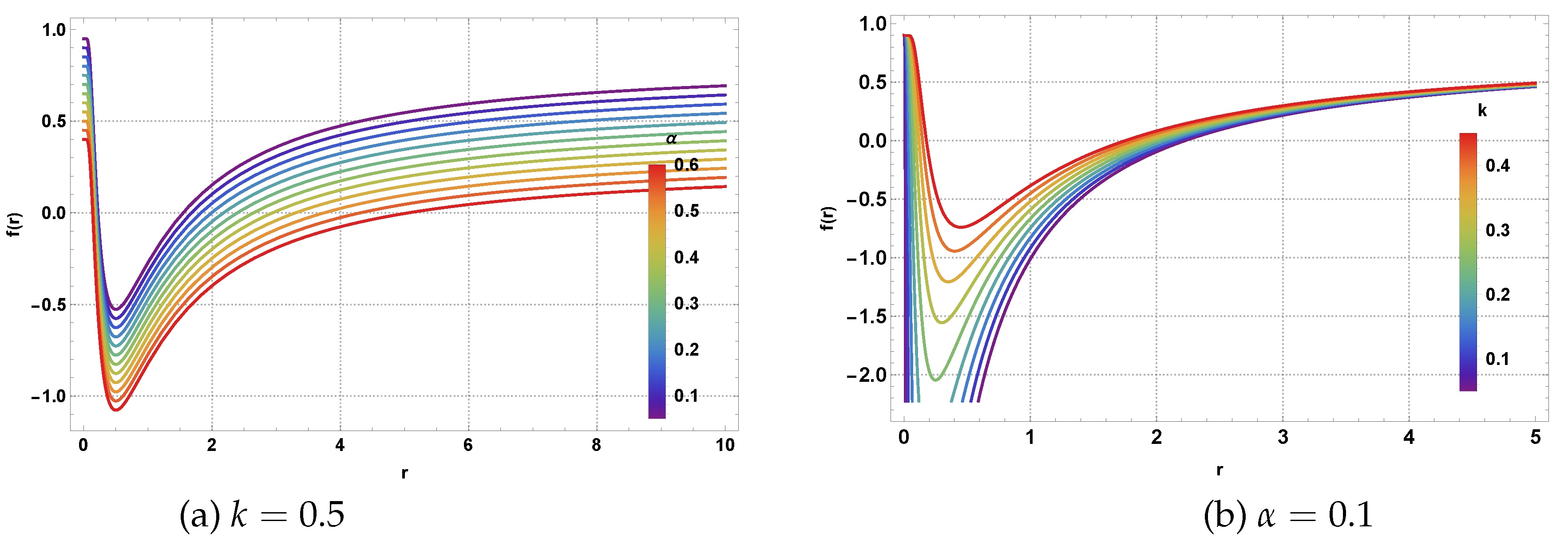
Figure 2.
Embedding diagrams of spherically symmetric AdS BHs with a CoS and QF in the NLED scenario. The common parameters are fixed to , , and . The plots show how the throat geometry and horizon position vary with the string parameter , nonlinear magnetic charge k, and quintessence normalization N. Red rings denote the event horizons located at . Parameter sets correspond to horizon structures in Table 1.
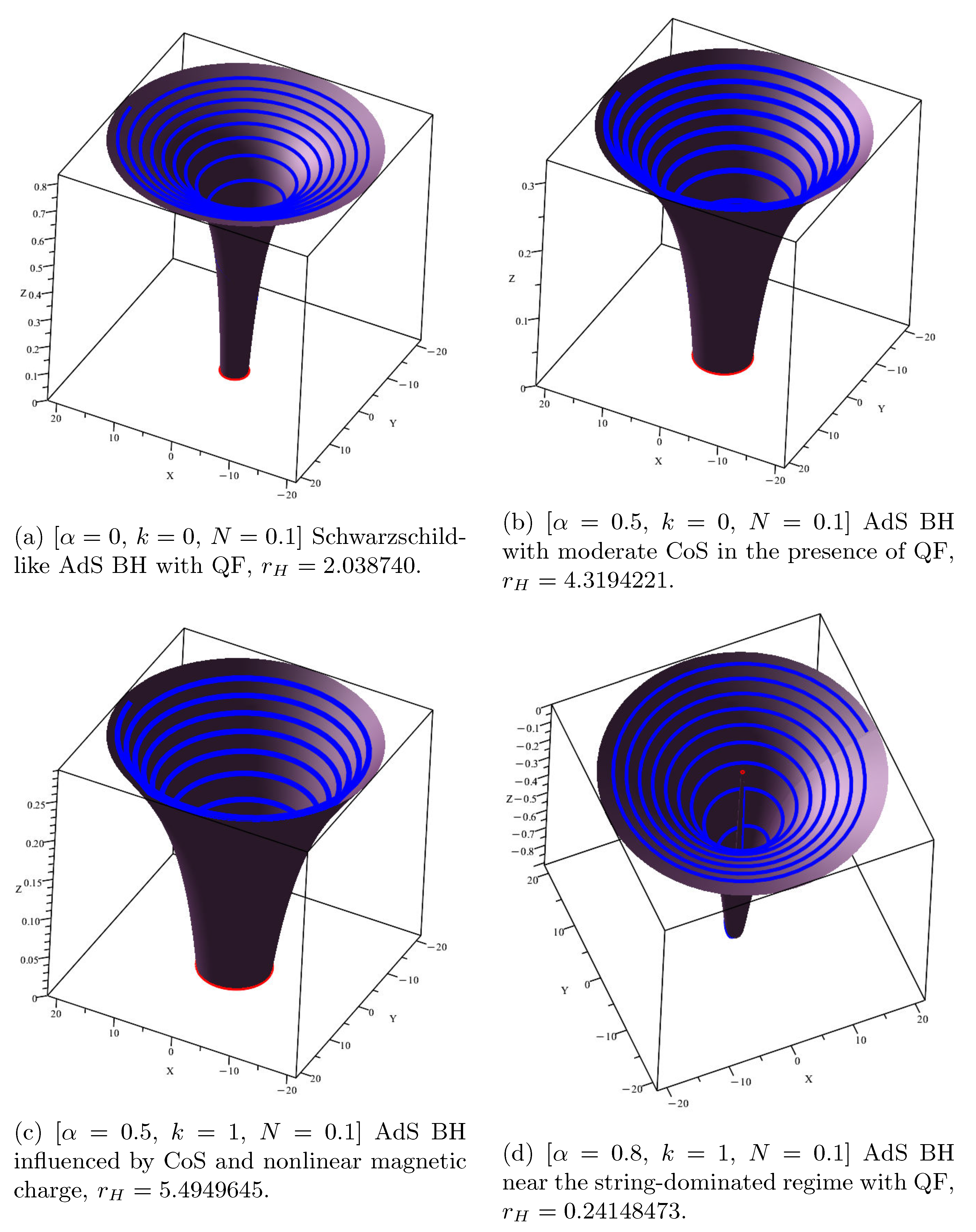
Figure 3.
Behavior of the effective potential as a function of r for different values of CoS parameter , state parameter w, and the magnetic charge k. Here .
Figure 3.
Behavior of the effective potential as a function of r for different values of CoS parameter , state parameter w, and the magnetic charge k. Here .
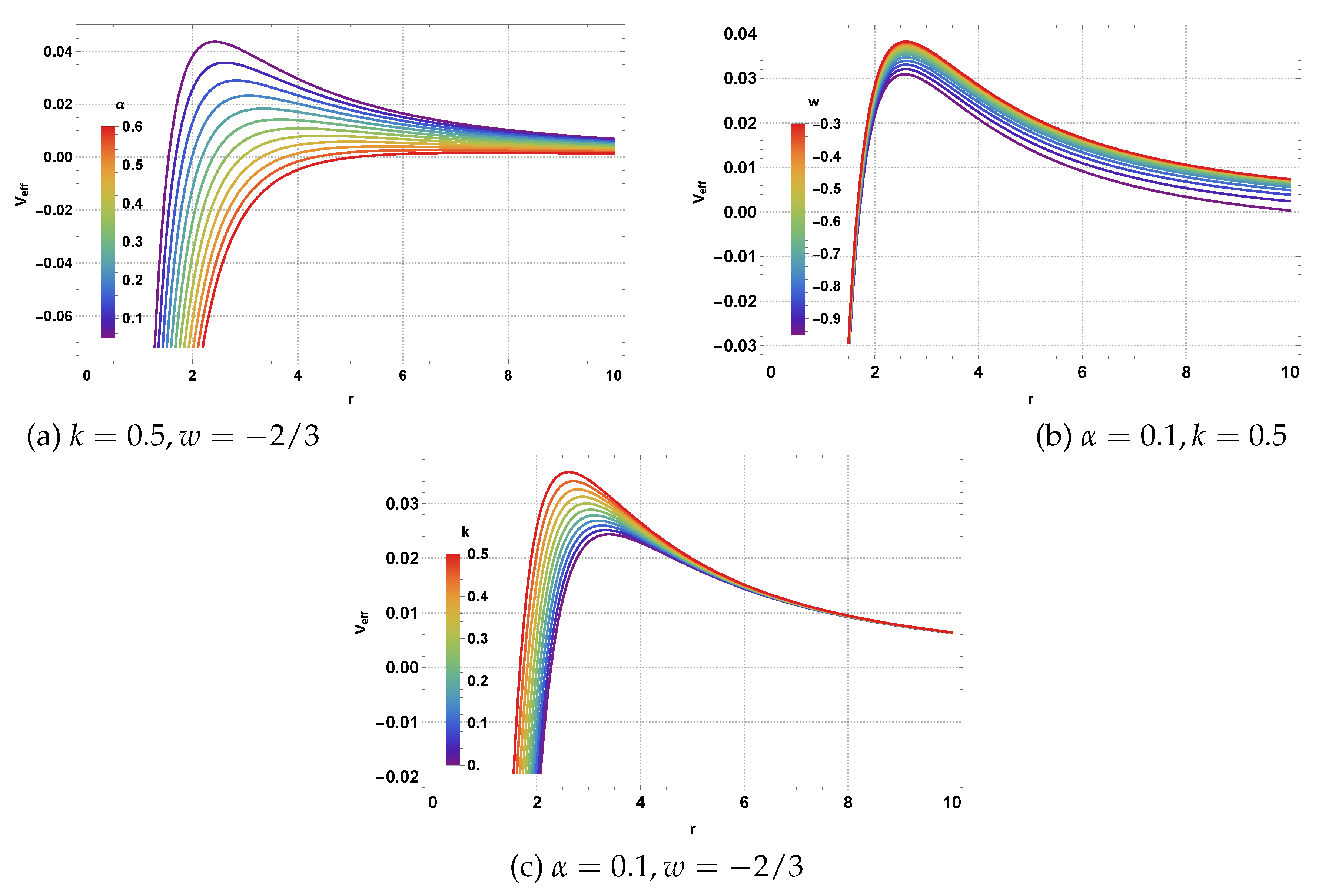
Figure 4.
Behavior of the effective radial force experienced by photon particles as a function of r for different values of CoS parameter and magnetic charge k. Here .
Figure 4.
Behavior of the effective radial force experienced by photon particles as a function of r for different values of CoS parameter and magnetic charge k. Here .
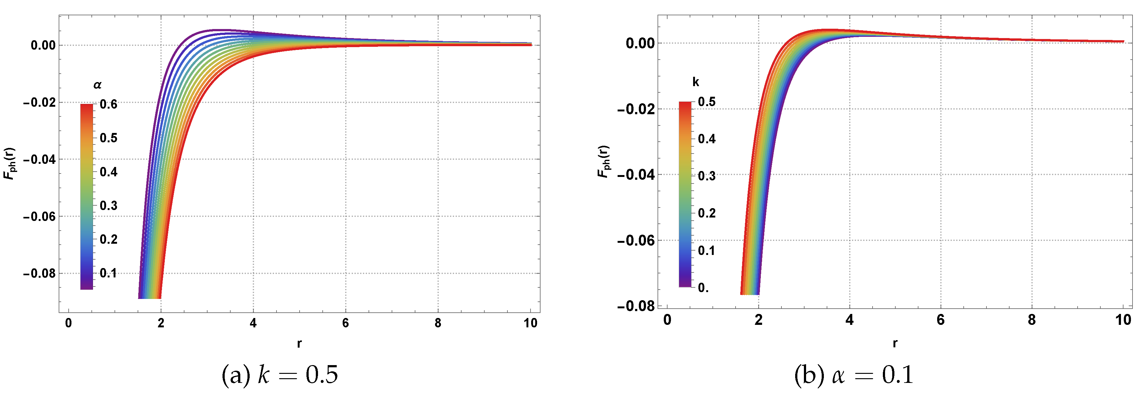
Figure 5.
Photon sphere radius as a function of and . Here .

Figure 6.
Shadow radius as a function of and . Here .
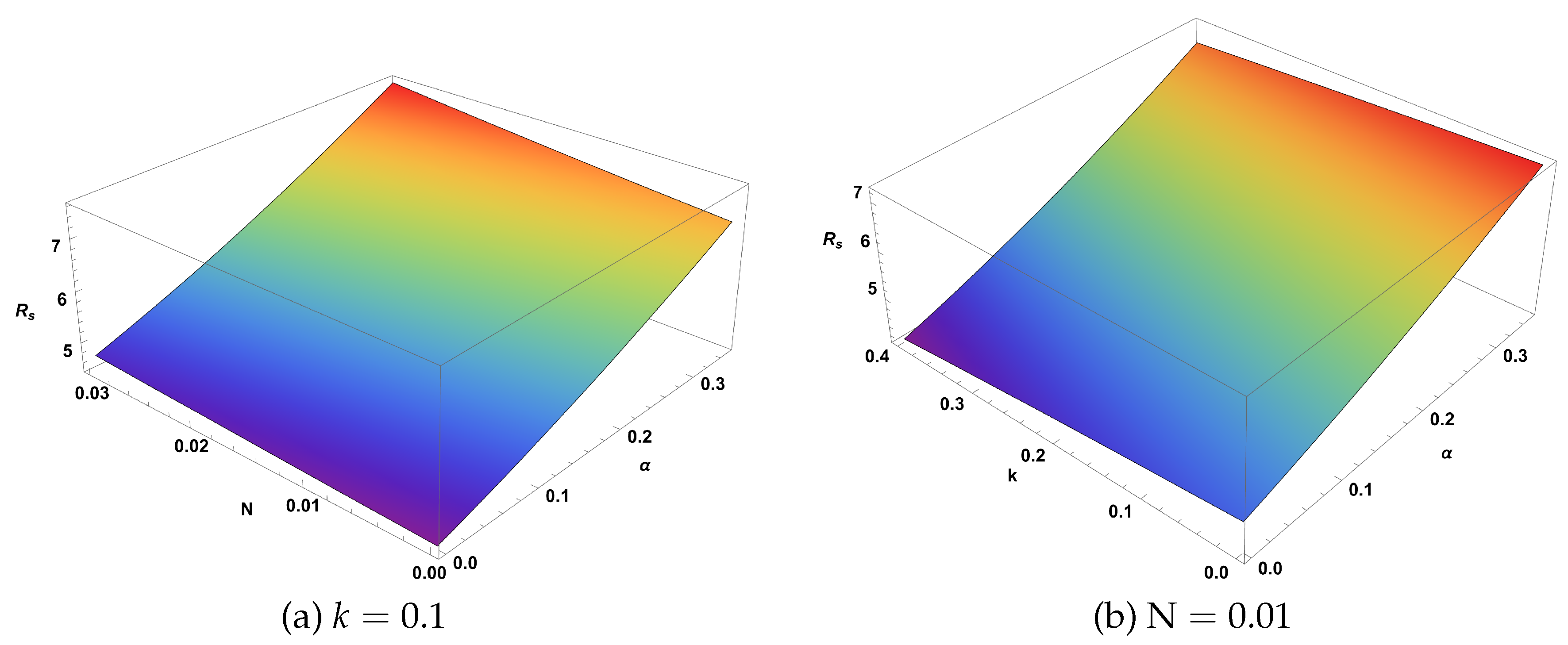
Figure 7.
Effects of CoS parameter , NLED parameter k, and QF constant on BH shadow size. Here, .
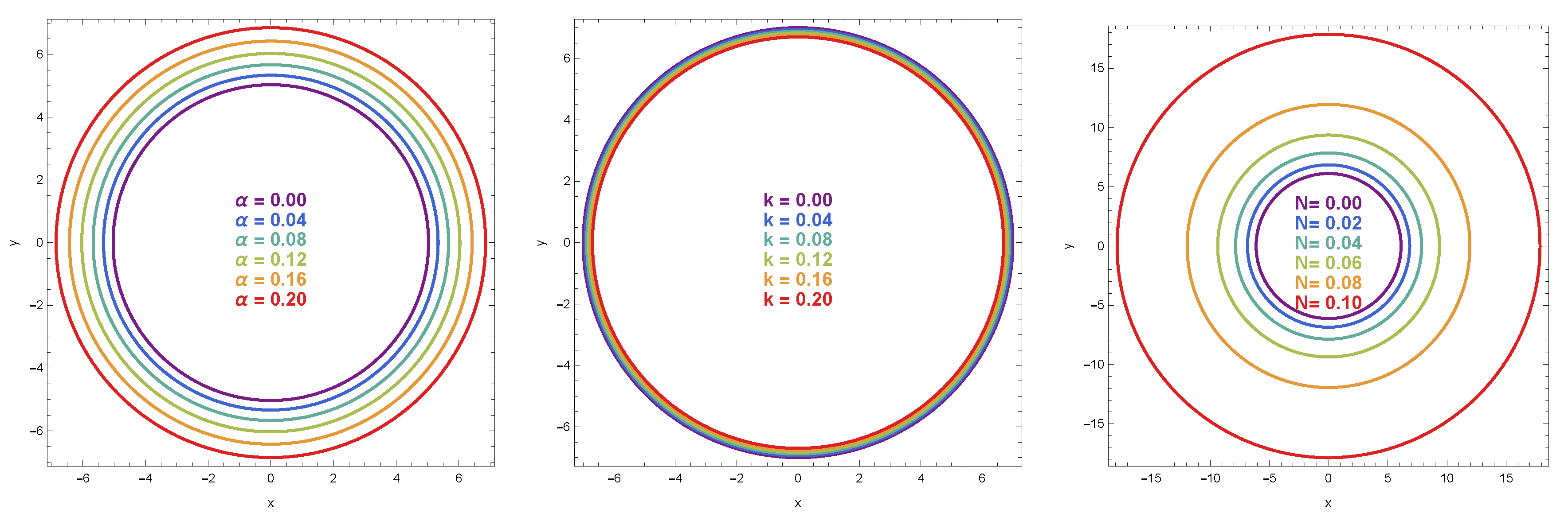
Figure 8.
Behavior of the Lyapunov exponent as a function of with different values of and k. Here .
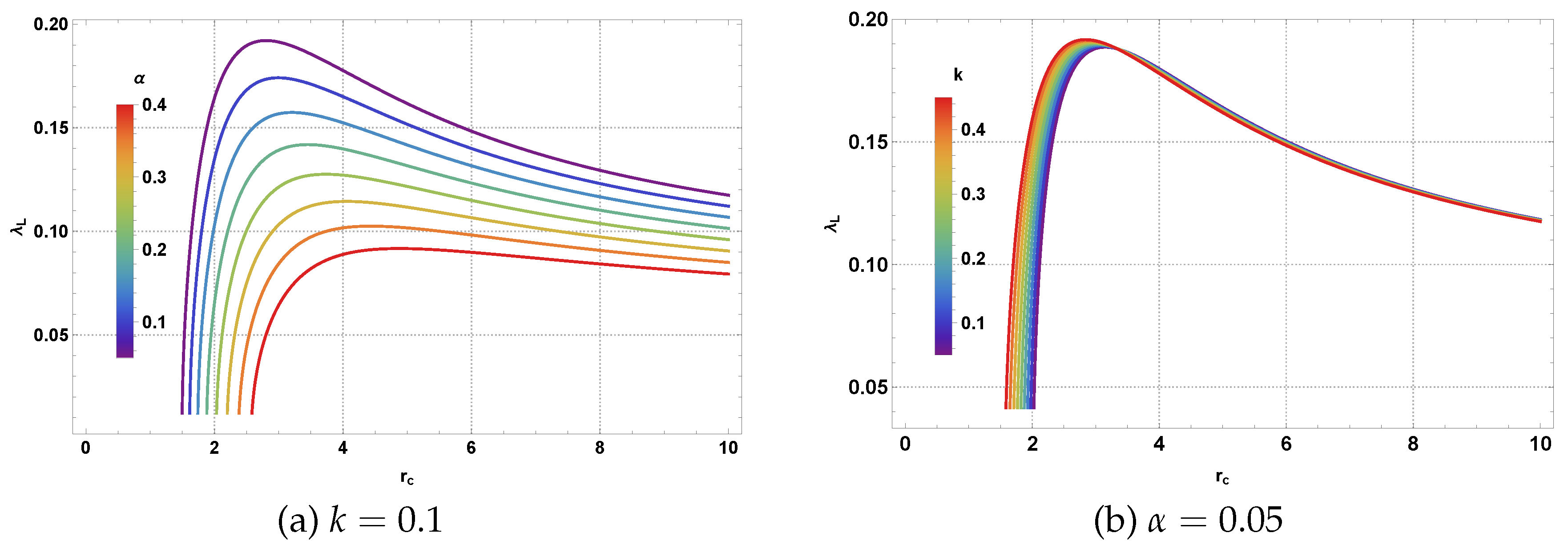
Figure 9.
Behavior of the potential function as a function of r for different values of CoS parameter , state parameter w, and the magnetic charge k. Here .
Figure 9.
Behavior of the potential function as a function of r for different values of CoS parameter , state parameter w, and the magnetic charge k. Here .
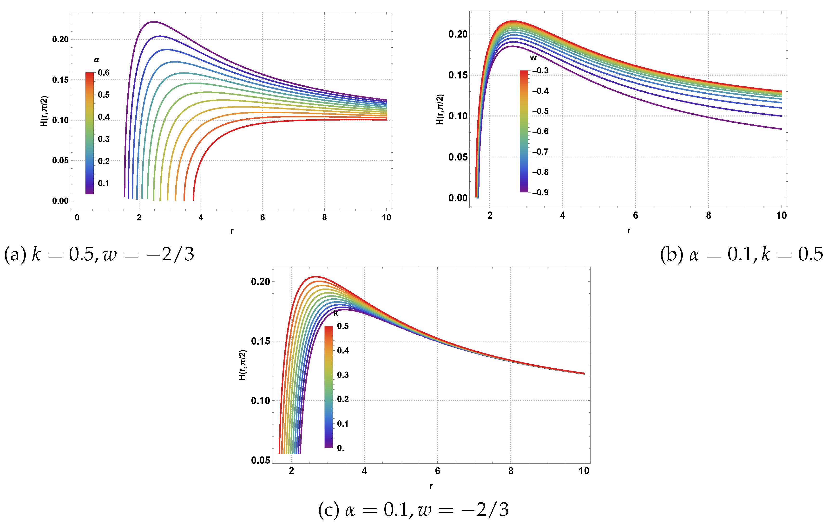
Figure 10.
The arrows represent the unit vector field on a portion of the plane. .
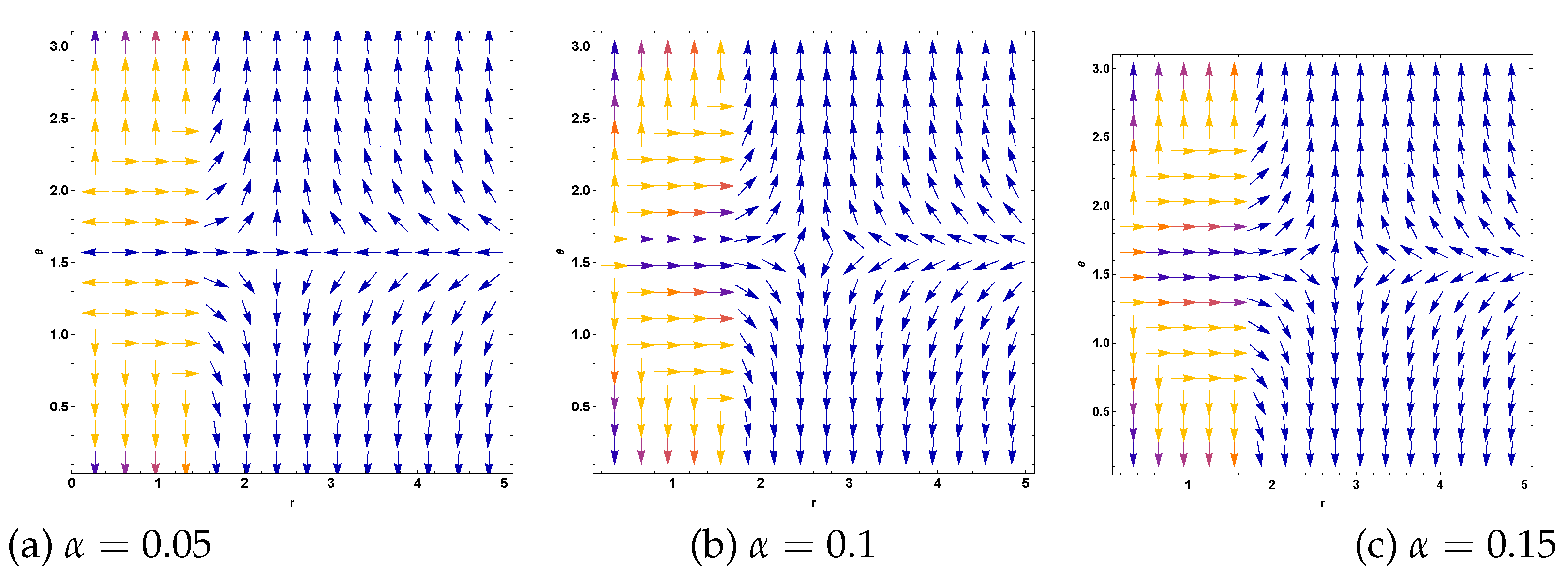
Figure 11.
The arrows represent the unit vector field on a portion of the plane. .
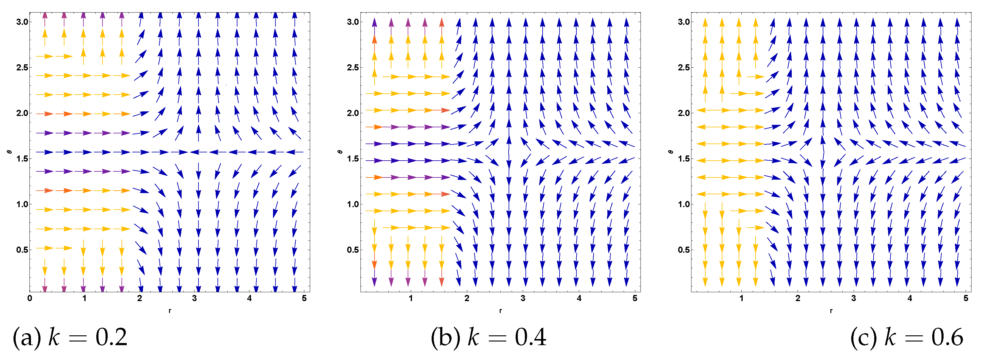
Figure 12.
The arrows represent the unit vector field on a portion of the plane. .

Figure 13.
Behavior of the effective potential as a function of r for different values of CS parameter , state parameter w, and the magnetic charge k. Here .
Figure 13.
Behavior of the effective potential as a function of r for different values of CS parameter , state parameter w, and the magnetic charge k. Here .
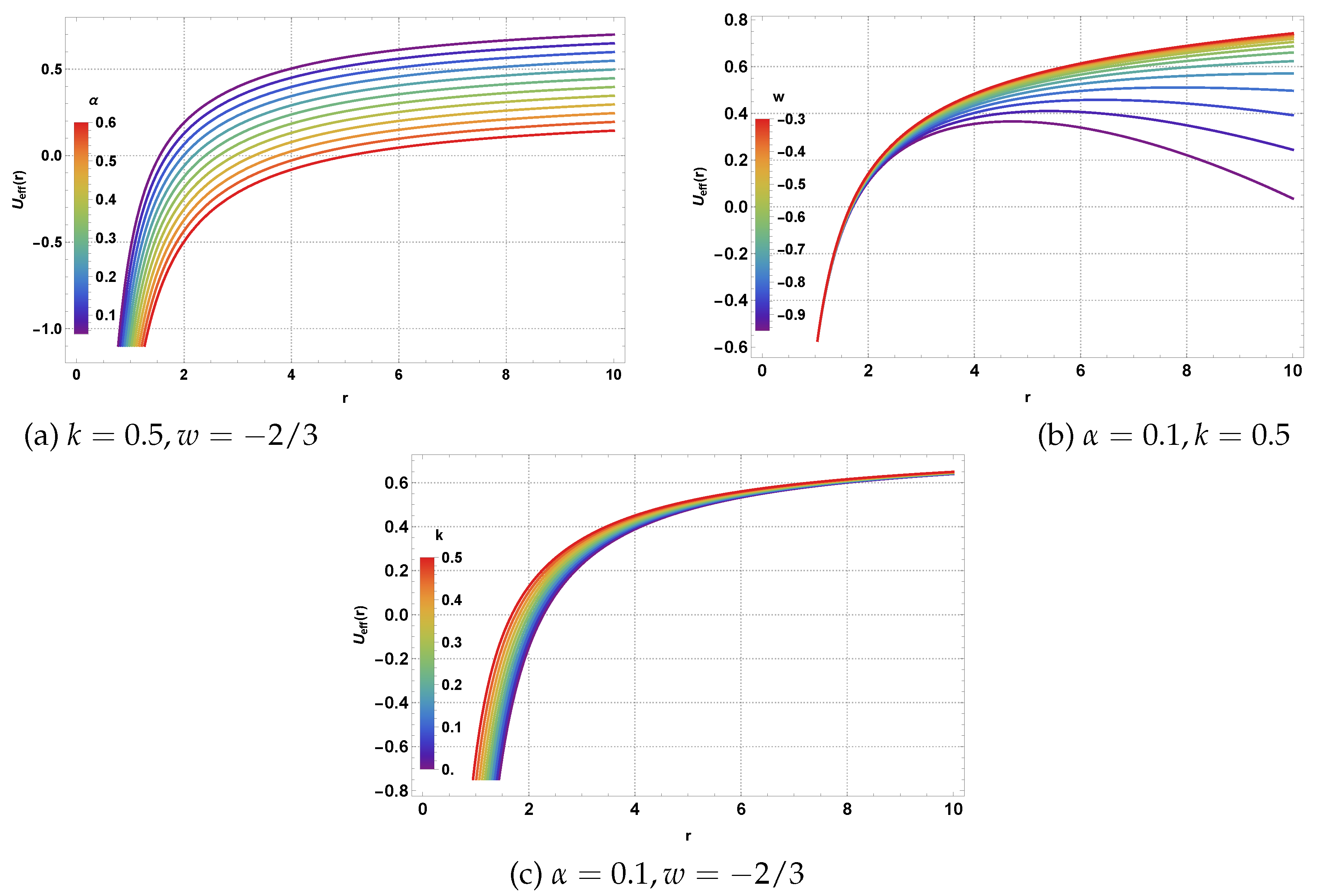
Figure 14.
Behavior of the specific angular momentum as a function of r for different values of CS parameter and magnetic charge k. Here .
Figure 14.
Behavior of the specific angular momentum as a function of r for different values of CS parameter and magnetic charge k. Here .
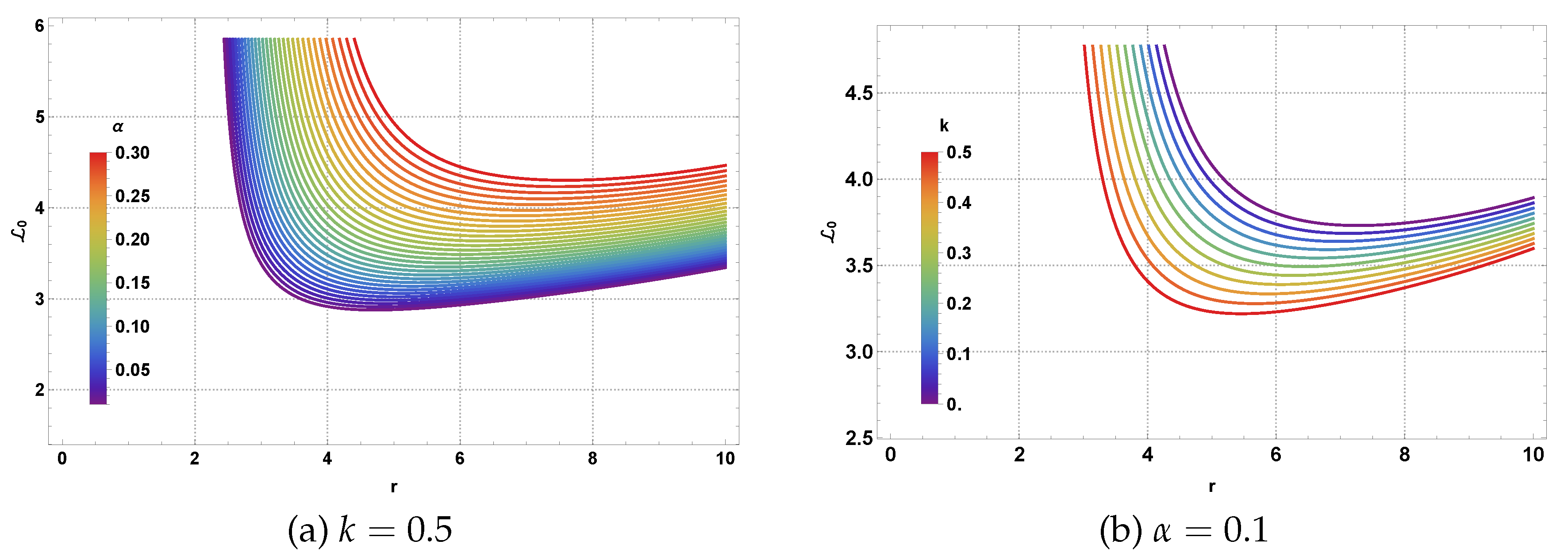
Figure 15.
Behavior of the specific energy as a function of r for different values of CoS parameter and magnetic charge k. Here .
Figure 15.
Behavior of the specific energy as a function of r for different values of CoS parameter and magnetic charge k. Here .
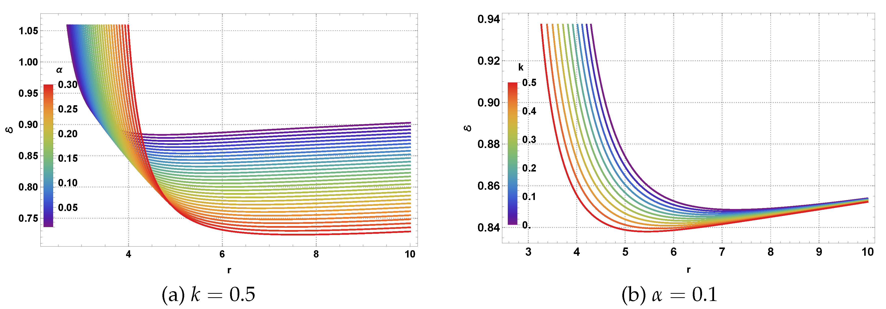
Figure 16.
3D plot of the ISCO radius as a function of . Here .
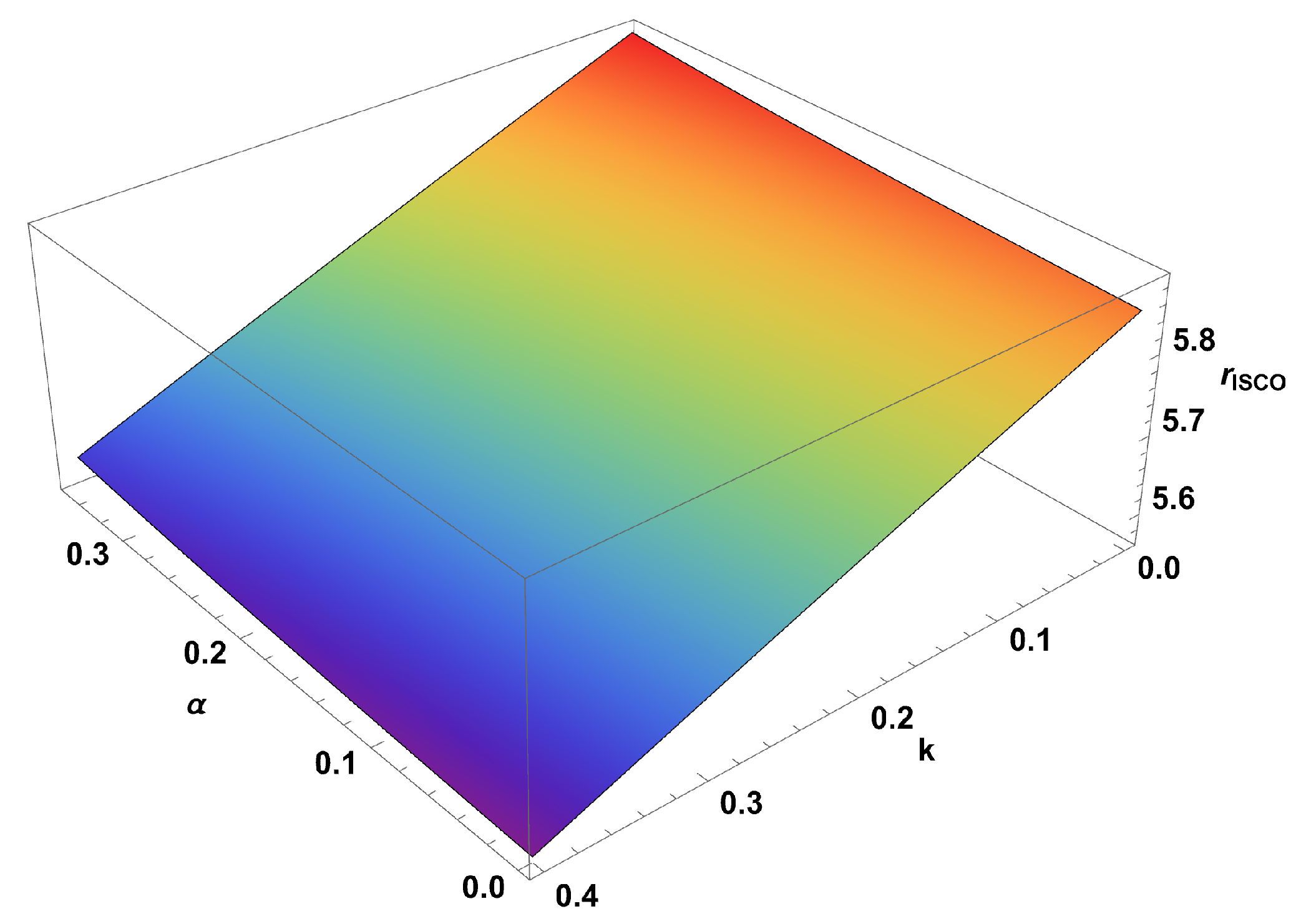
Figure 17.
Behavior of the effective radial force experienced by neutral test particles as a function of r for different values of CoS parameter and magnetic charge k. Here
Figure 17.
Behavior of the effective radial force experienced by neutral test particles as a function of r for different values of CoS parameter and magnetic charge k. Here
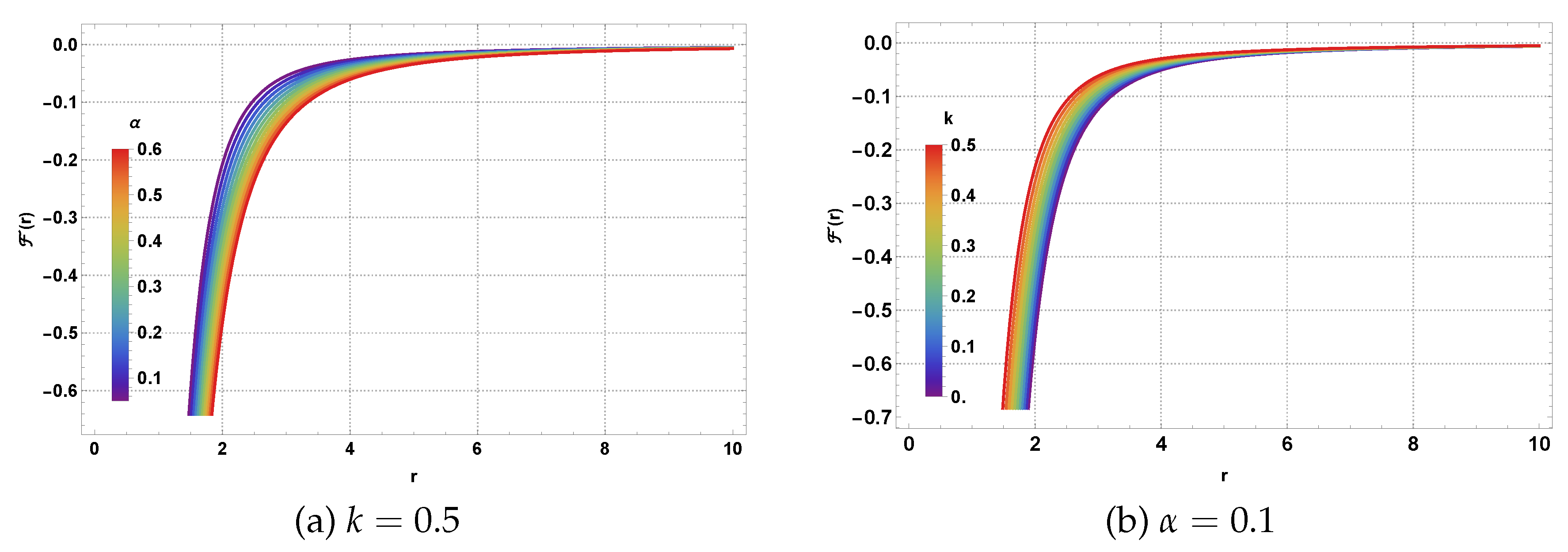
Figure 18.
Behavior of the radial frequency as a function of for different values of and k. Here .
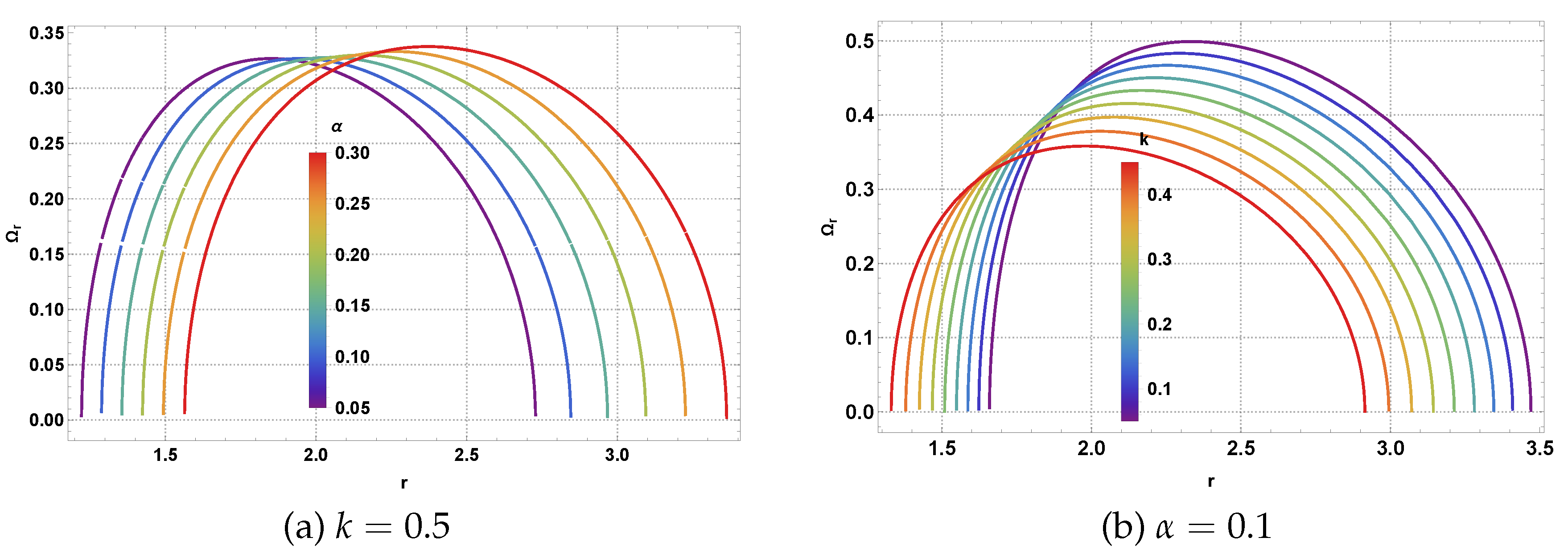
Figure 19.
Behavior of the vertical angular frequency as a function of for different values of and k. Here .
Figure 19.
Behavior of the vertical angular frequency as a function of for different values of and k. Here .
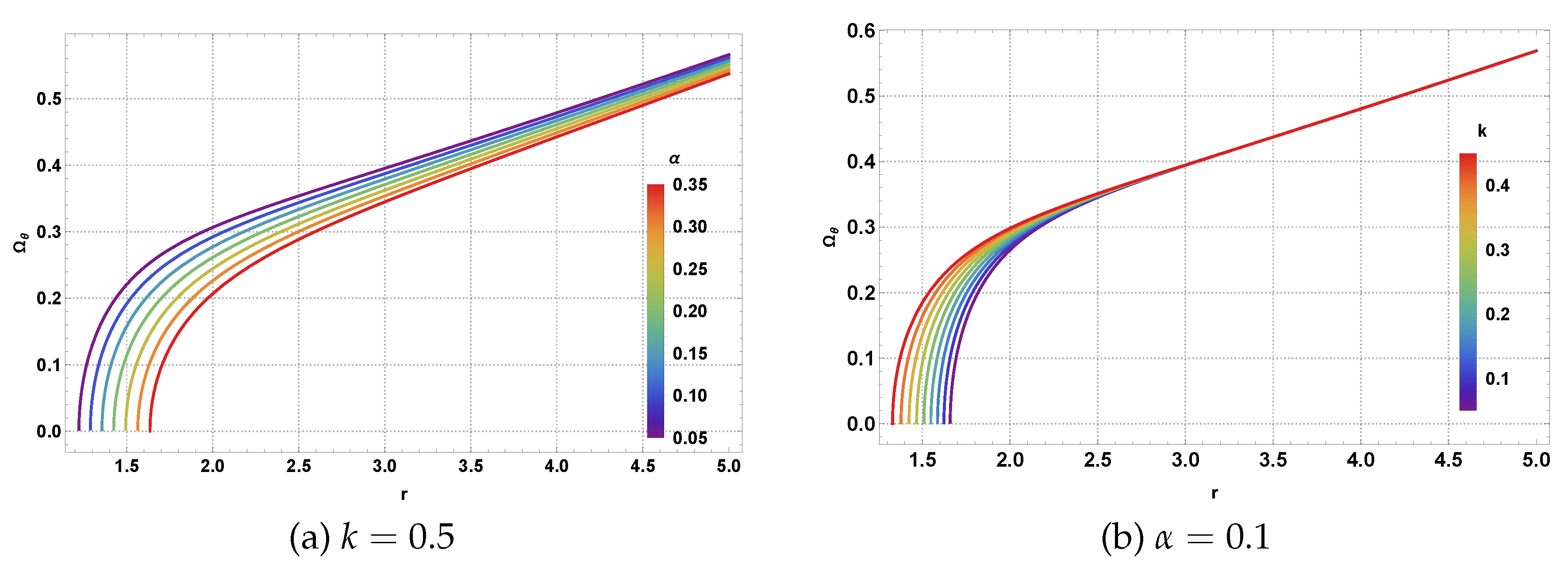
Figure 20.
Behavior of the azimuthal frequency as a function of for different values of w and k. Here .
Figure 20.
Behavior of the azimuthal frequency as a function of for different values of w and k. Here .
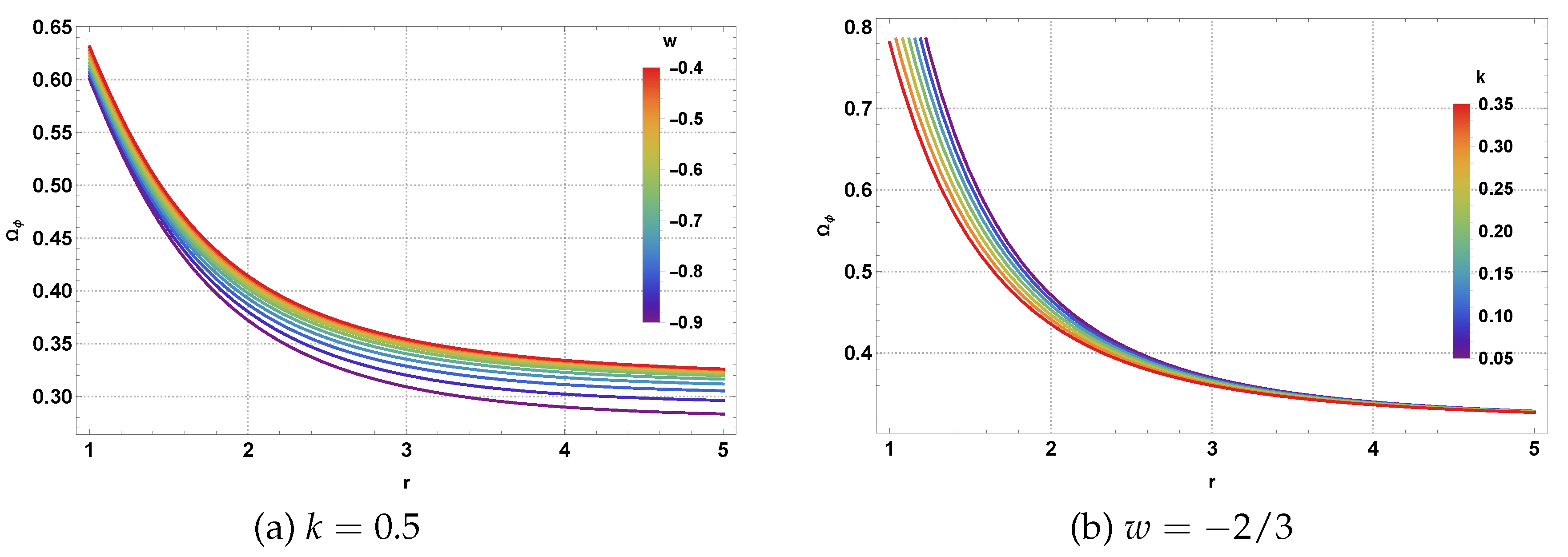
Figure 21.
Behavior of the periastron precession frequency in the equatorial plane by varying NLED parameter k for different set of CoS parameter . Here, we set .
Figure 21.
Behavior of the periastron precession frequency in the equatorial plane by varying NLED parameter k for different set of CoS parameter . Here, we set .
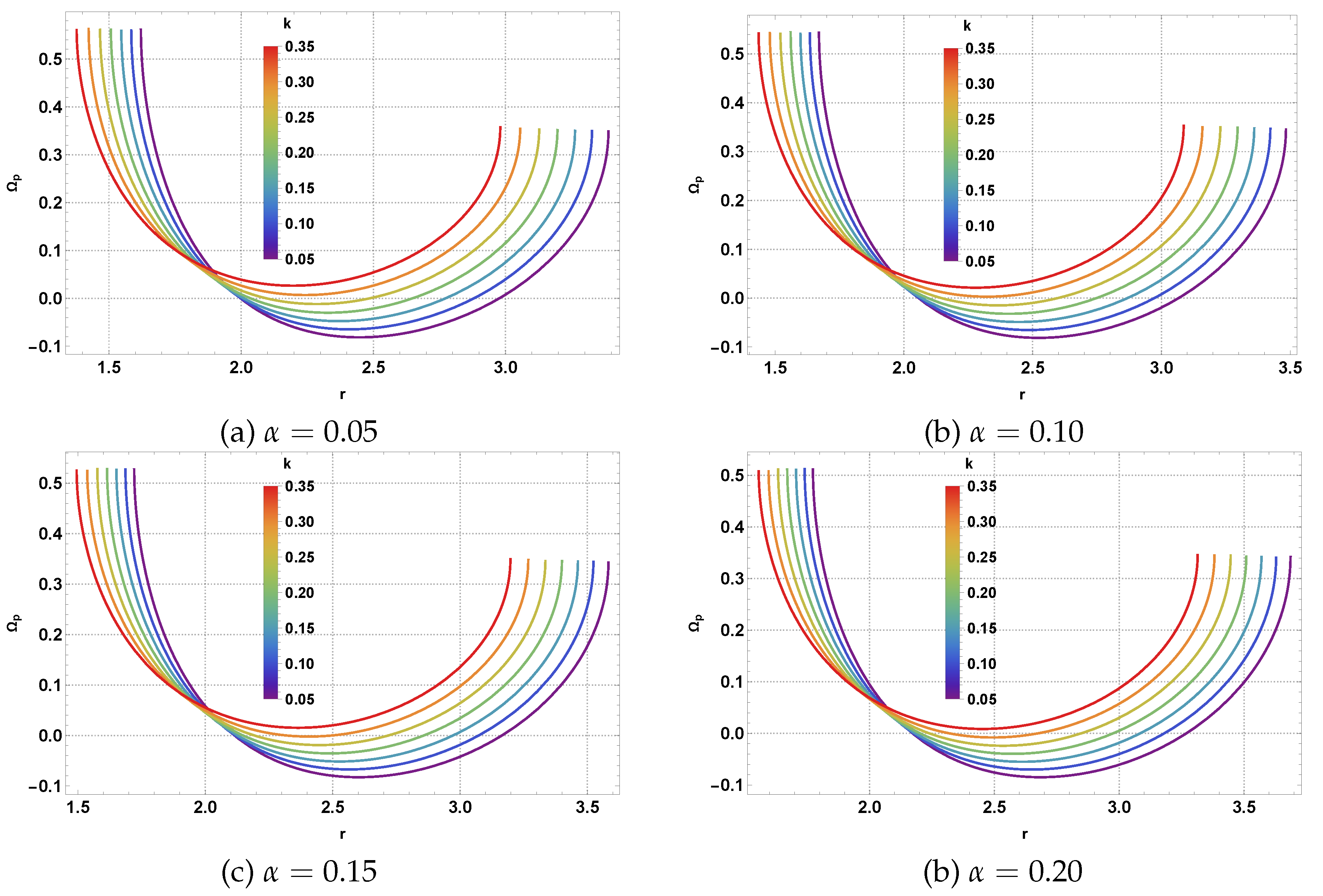
Figure 22.
Behavior of the periastron precession frequency in the equatorial plane by varying NLED parameter k for different set of CoS parameter . Here, we set .
Figure 22.
Behavior of the periastron precession frequency in the equatorial plane by varying NLED parameter k for different set of CoS parameter . Here, we set .
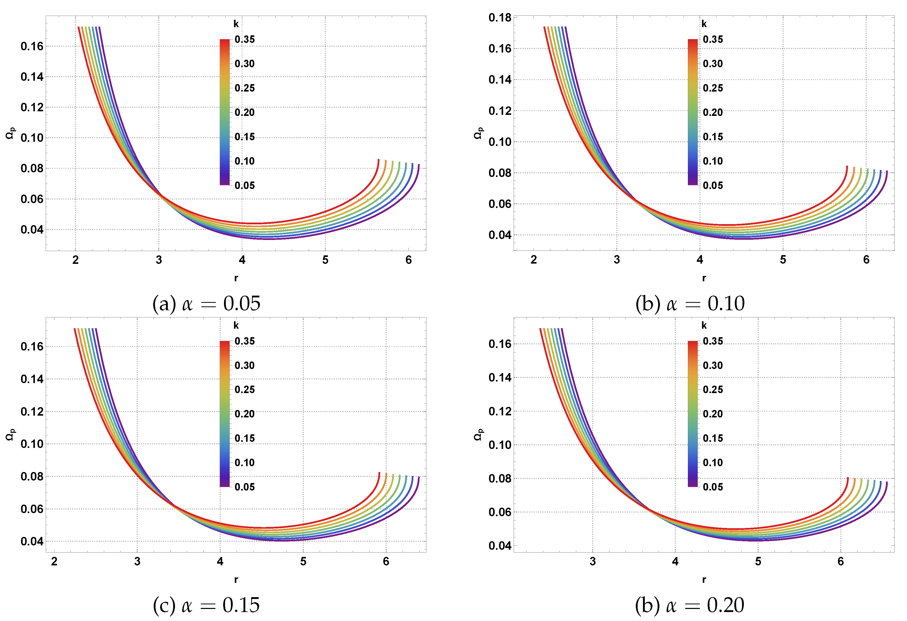

Table 1.
Horizon structure of a BH spacetime governed by the metric function , where is the global monopole parameter, k encodes exponential regularization effects, N is the quintessence normalization constant, and w is the quintessence state parameter. The CC is taken to be negative (), and M varies across the table. For each configuration, the number and type of horizons (extremal, non-extremal, or absence of horizon) are shown. The data highlights how tuning , k, and M reshapes the causal structure in the presence of both quintessence (, ) and asymptotically AdS behavior.
| M | k | Horizon(s) | Configuration | |
|---|---|---|---|---|
| M | k | Horizon(s) | Configuration | |
| 0.5 | 0.0 | 0.0 | Extremal or Single Root BH | |
| 0.5 | 0.0 | 0.5 | No horizon (naked singularity) | |
| 0.5 | 0.1 | 0.0 | Extremal or Single Root BH | |
| 0.5 | 0.1 | 0.5 | No horizon (naked singularity) | |
| 0.5 | 0.2 | 0.0 | Extremal or Single Root BH | |
| 0.5 | 0.2 | 0.5 | No horizon (naked singularity) | |
| 0.5 | 0.5 | 0.0 | Extremal or Single Root BH | |
| 0.5 | 0.5 | 0.5 | Non-extremal BH | |
| 0.5 | 0.5 | 1.0 | No horizon (naked singularity) | |
| 0.5 | 0.8 | 0.0 | Extremal or Single Root BH | |
| 0.5 | 0.8 | 0.5 | Non-extremal BH | |
| 1.0 | 0.0 | 0.0 | Extremal or Single Root BH | |
| 1.0 | 0.0 | 0.5 | Non-extremal BH | |
| 1.0 | 0.0 | 1.0 | No horizon (naked singularity) | |
| 1.0 | 0.1 | 0.5 | Non-extremal BH | |
| 1.0 | 0.1 | 1.0 | No horizon (naked singularity) | |
| 1.0 | 0.2 | 0.0 | Extremal or Single Root BH | |
| 1.0 | 0.2 | 0.5 | Non-extremal BH | |
| 1.0 | 0.2 | 1.0 | No horizon (naked singularity) | |
| 1.0 | 0.5 | 0.0 | Extremal or Single Root BH | |
| 1.0 | 0.5 | 0.5 | Non-extremal BH | |
| 1.0 | 0.8 | 0.0 | Extremal or Single Root BH | |
| 1.0 | 0.8 | 0.5 | Non-extremal BH | |
| 1.5 | 0.0 | 0.0 | Extremal or Single Root BH | |
| 1.5 | 0.0 | 0.5 | Non-extremal BH | |
| 1.5 | 0.1 | 0.0 | Extremal or Single Root BH | |
| 1.5 | 0.1 | 0.5 | Non-extremal BH | |
| 1.5 | 0.1 | 1.0 | Non-extremal BH | |
| 1.5 | 0.2 | 0.0 | Extremal or Single Root BH | |
| 1.5 | 0.2 | 0.5 | Non-extremal BH | |
| 1.5 | 0.5 | 0.0 | Extremal or Single Root BH | |
| 1.5 | 0.5 | 1.0 | Non-extremal BH | |
| 1.5 | 0.8 | 0.0 | No horizon (naked singularity) | |
| 1.5 | 0.8 | 1.0 | Extremal or Single Root BH |
Table 2.
Numerical values of the photon sphere radius and shadow radius for various values of , and N. Constants used: , , .
Table 2.
Numerical values of the photon sphere radius and shadow radius for various values of , and N. Constants used: , , .
Table 3.
Photon sphere and shadow radius under different parameter assumptions.
| Case | Photon Sphere Equation | Shadow Radius |
|---|---|---|
| [54] | ||
| [18] | ||
| [9] | ||
| [55] |
Table 4.
Numerical values of the ISCO radius for various values of , and N. Constants used: , , .
Disclaimer/Publisher’s Note: The statements, opinions and data contained in all publications are solely those of the individual author(s) and contributor(s) and not of MDPI and/or the editor(s). MDPI and/or the editor(s) disclaim responsibility for any injury to people or property resulting from any ideas, methods, instructions or products referred to in the content. |
© 2025 by the authors. Licensee MDPI, Basel, Switzerland. This article is an open access article distributed under the terms and conditions of the Creative Commons Attribution (CC BY) license (http://creativecommons.org/licenses/by/4.0/).
Copyright: This open access article is published under a Creative Commons CC BY 4.0 license, which permit the free download, distribution, and reuse, provided that the author and preprint are cited in any reuse.


