
Submitted:
06 October 2025
Posted:
08 October 2025
Read the latest preprint version here
Abstract
In this book, we present a mathematically consistent paradigm for describing nature. Modern physics is supported by an immense body of experimental and observational data, alongside a theoretical framework that, at times, aligns with this data—and at other times, diverges from it. The absence of a clear theoretical explanation for the cause of quantum phenomena, combined with the growing mismatch between cosmological observations and theoretical predictions, suggests that a fundamental principle of nature is missing from current physical theories. The Self-Variation Theory introduces such a principle into the theoretical foundations of physics.In this work, we present the core principles and primary consequences of SVT. The theory is built upon three foundational elements:the Principle of Self-Variation,the Principle of Conservation of Energy-Momentum, and a definition of the rest mass for fundamental particles.From these principles, Self-Variation Theory leads to a number of key conclusions:it predicts a specific internal structure of particles that extends across all distance scales,it provides a unified explanation for particle interactions,it accounts for both cosmological data and quantum phenomena, offering a coherent framework that connects them. The theory's predictions regarding the origin, evolution, and current state of the universe are in agreement with available observational evidence. From subatomic scales to astronomical distances spanning billions of light-years, Self-Variation Theory demonstrates a remarkable consistency with experimental and observational data. The structure of the book has been carefully designed to ensure the necessary clarity and precision in presenting the theory. A sequence of interconnected derivations begins with the fundamental principles, proceeds through their synthesis, and culminates in the field equations of the theory—applicable across all distance scales.
Keywords:
electromagnetism
; gravity
; cosmology
; quantum mechanical operators
1. Introduction
This chapter introduces the central idea of Self-Variation Theory: the principle of self-variation, a new physical principle absent from existing theories. According to this principle, the rest mass and, more generally, the self-variating charge of fundamental particles undergo a systematic increase over time.
In compliance with the conservation of energy and momentum, this increase necessarily leads to the emission of energy–momentum into the surrounding spacetime. This emitted energy–momentum is not incidental—it constitutes the origin of interactions between material particles. Thus, gravitational and electromagnetic interactions emerge naturally as consequences of the self-variation of rest mass and electric charge, respectively.
The chapter formalizes the theory’s three foundational principles:
The principle of self-variation,
The principle of energy–momentum conservation, and
A rigorous definition of rest mass.
The mathematical framework and key symbols are introduced, and several immediate consequences of the theory are derived. The chapter concludes with a summary of major theoretical predictions, highlighting the scope of Self-Variation Theory, which leads to hundreds of novel equations and a wide range of new insights across all domains of physics.
1.1. Axiomatic Foundation of Self-Variation Theory
In a N-dimensional Riemannian spacetime [1,2,3,4,5] the Self-Variation Theory is based on three principles [6,7,8], the principle of self-variation, the principle of conservation of energy-momentum and a definition of the rest mass of fundamental particles. We present the three principles of the Theory.
1. The self-variation principle
With the term “self-variation principle” we mean an exactly determined increase of the rest mass of material particles. Moreover the self-variation principle generally applies to all kind of charges of the fundamental particles. Direct consequence of the principle of self-variation is that energy, momentum and charge (if the particle is charged) are distributed in the surrounding spacetime. For example, to compensate for the increase, in absolute value, of the negative electric charge of the electron, the particle emits a corresponding positive electric charge into the surrounding spacetime. As a consequence of this emission the total electric charge is conserved. Similarly, the increase of the rest mass of the material particle involves the “emission” of negative energy as well as momentum in the spacetime surrounding the material particle (spacetime energy-momentum) .
We generally denote the rest mass or charge of particle with . The principle of self-variation quantitatively describes the interaction of the ‘self-variation charges’. Let
be the self-variating charge and let be the energy-momentum the particle emit in spacetime as a consequence of the self-variation of the charge . The self-variation principle asserts that valid
(1.1)
in every system of reference
where is the reduced Planck constant and , is a constant. denotes the momentum and the time measured by an observer, where is vacuum velocity of light and is the imaginary unit, . If , where is the rest mass of a particle Equation (1) becomes
. (1.2)
The principle of self-variation quantitatively describes the interaction of material particles with the spacetime energy-momentum. For the formulation of the equations the following symbolism is used,
is the energy of the particle,
is the momentum of the particle,
is the rest mass of the particle,
is the energy of the spacetime energy-momentum related to the particle,
is the momentum of the spacetime energy-momentum related to the particle,
is the rest energy of the spacetime energy-momentum related to the particle. We define the N-vectors,
, (1.3)
, (1.4)
, (1.5)
, (1.6)
where, .
In Equation (1.1), the momentum of the particle is due to the charge . The momentum arises as a consequence of the self-variation of the charge . The physical quantities , , are determined at the same point of spacetime.
2. The principle of conservation of energy-momentum
The material particle and the spacetime energy-momentum with which the material particle interacts comprise a dynamic system, which we call “generalized particle”. We consider the covariant momentum of the particle , the momentum of spacetime and the total momentum of generalized particle,
, . (1.7)
Equation (1.7) expresses the energy-momentum conservation of the generalized particle in a N-dimensional spacetime. As a consequence of Equation (1.1), the N-vectors , and are covariant. According to the self-variation principle the N-vector is non-zero, .
3. The rest mass of the material particles
As invariant physical quantities, the rest masses corresponding to the N-vectors , , are given by the following equations,
, (1.8)
, (1.9)
. (1.10)
For the contravariant N-vectors we have , , where is the metric tensor. The N-vector is constant, therefore rest mass is also constant. In Equations (1.8), (1.9), (1.10) we follow Einstein's summation convention for terms where an index appears twice.
The goal of Self-Variation Theory is to find the functions , , and . The differential equations resulting from the axiomatic foundation of the Theory give specific solutions for these functions. These solutions have a common feature. The material particle has structure, even if we assume it to be a point. In the context of the Self-Variation Theory, the generalized particle replaces the concept of the material particle.
We now present three direct consequences of the principles of the Theory. The first of these is given by the following equations,
, (1.11)
. (1.12)
Proof.
From Equation (1.1) we get
where with we denote the covariant derivative with respect to . Then we get,
and equivalently we get,
and with Equation (1.1) we get,
and finally we obtain,
Similarly, from the equation
we get,
Therefore we have
and taking into consideration that we get Equation (1.11). From Equations (1.11) and (1.7) we get Equation (1.12). In the proof process we used the symbols of Christoffel,
1.2. Self-Variation of the Rest Mass
If , the rest mass is self-variating. The principle of self-variation applies to rest mass . Therefore, for each solution , , and that we get from the differential equations of the Theory, one of the following equations holds,
, (1.13)
or
. (1.14)
In Section 2.2 Equation (1.4) is derived. The case (1.13) has not appeared in the investigation of the equations of Self-Variation Theory so far. It is quite possible that Equation (1.14) has general validity.
1.3. The Relative Position of N-Vectors and
The relative position of N-vectors and in spacetime can be given by the following equations,
(1.15)
where . Denoting the matrix ,
(1.16)
Equation (1.13) is written in the form
. (1.17)
1.4. Main Conclusions of the Self-Variation Theory
We present the main conclusions of the Self-Variation Theory. In the next five Chapters we successively present the consequences of self-variation in flat spacetime, the electromagnetic interaction, the gravitational interaction, the cosmological scale equations and the justification of cosmological data, the consequences of self-variation in the microscopic scale and the justification of quantum phenomena. The Self-Variation Theory gives a large number of conclusions. In this introductory Section, indicatively, after the abstract of each Chapter we present some of its equations, graphs or corollaries.
In Chapter 2 we study the generalized particle in the flat 4-dimensional spacetime of Special Relativity. This study is fundamental, since it highlights the basic consequences of the self-variation of material particles. In the last Section of the Chapter we do the corresponding study in N-dimensional curved spacetime.
The main conclusion of the Chapter is the Internal Symmetry Theorem. This Theorem gives the rest mass and in general the charge of a particle as a function of spacetime. It also gives the relation of the energy-momentum and rest mass of a particle to the energy-momentum and rest mass in the surrounding spacetime of the particle. If the particle is charged, the Theorem gives a distribution of charge in the surrounding spacetime of the particle.
The Internal Symmetry Theorem justifies the so far known cosmological data in a flat and static universe. This justification is made by Equation (2.31) for the rest mass of material particles,
and of its general expression
as given by Equation (2.33) for the charge . The notation we follow in these Equations is given in Chapter 2. The analytical justification of the cosmological data is done in Chapter 5.
In Chapter 3, we present a new class of potentials—referred to as self-variation potentials—that are compatible with the self-variation principle and replace the traditional Liénard–Wiechert potentials in the surrounding spacetime of a point electric charge.
We study the electromagnetic field generated by a point electric charge undergoing arbitrary motion within an inertial frame of reference. This analysis leads to the substitution of the Liénard–Wiechert potentials by the self-variation potentials. Although both sets of potentials yield identical electromagnetic fields, they differ in their foundational principles and compatibility with physical laws.
Specifically:
The self-variation potentials are fully compatible with both the Lorentz–Einstein transformations and the self-variation principle.
The Liénard–Wiechert potentials, while compatible with the Lorentz–Einstein transformations, are not compatible with the self-variation principle when considered in the surrounding spacetime of a point charge.
Maxwell’s equations, as is well-known, are compatible with Lorentz invariance. In this chapter, we demonstrate that they are also compatible with the self-variation principle. Therefore, the fundamental laws of physics can be extended to incorporate self-variation.
Let us denote:
By , the set of equations compatible with Lorentz–Einstein transformations, and
by , the set of equations compatible with the self-variation of electric charge, then we have: .
This means that Self-Variation Theory introduces additional constraints on the laws of physics beyond those imposed by Special Relativity.
In this chapter, we perform precise calculations to determine the consequences of self-variation in the spacetime surrounding a point charge . One key result is that an effective distribution of opposite electric charge appears in the surrounding spacetime due to self-variation. We compute both the electric charge density and the current density associated with this effect.
Furthermore, a geometric consequence of self-variation is established through the Orbit Representation Theorem. For each spatial direction, the trajectory (orbit) of the charge is mapped to a corresponding curve in the surrounding spacetime. The theorem relates the tangent vector, curvature, and torsion of these two curves, establishing a deep geometric link between the charge's motion and the structure of the surrounding spacetime.
the same as all the corresponding electromagnetic potentials in classical electromagnetism [15,16,17,18,19,20,21,22,23,24,25,26,27,28,29], are inversely proportional to the distance from the field source. The self-variation electromagnetic potential [6,7,8], [30],
adds an extra term to the electromagnetic potential,
which is independent of the distance . This term makes the electromagnetic potential compatible with self-variation, and paves the way for the correlation of electromagnetics with the gravitational interaction. The notation we follow in these Equations is given in Chapter 3.
In Chapter 3 we have a precise calculation for the consequences of self-variation in the surrounding spacetime of . As a consequence of the self-variation, an electric charge of opposite sign on is distributed in the surrounding spacetime of the electric charge . We calculate the electric charge density and the current density in the surrounding spacetime of . This is a direct consequence of self-variation, a characteristic prediction in the surrounding spacetime of that clearly shows the difference of the Self-Variation Theory from the Theories of twentieth century physics. Quantitatively, the charge density and the current density (refer to Equations (3.47)) are given by Equations,
The notation we follow in these Equations is given in Chapter 3.
In Chapter 4, we formulate the gravitational field equations within the framework of the Self-Variation Theory. A central feature of Self-Variation Theory is that it describes both gravity and electromagnetism using a unified set of equations. These equations govern the fields generated by the rest mass and/or electric charge of a particle.
The core equation of the theory establishes a relationship among three fundamental physical quantities: the rest mass (or electric charge) of the source, its relative velocity with respect to the observer, and the propagation speed of the field as measured by the observer. These velocities are directly linked to the observed field potential and field strength.
Initial analytical results show that the theory remains consistent across the range of distance scales for which we have observational data. Notably, Self-Variation Theory predicts enhanced rotational velocities of stars in galaxies, as well as galaxies within galaxy clusters—phenomena typically attributed to dark matter.
According to the field equations derived in Self-Variation Theory, gravity behaves differently depending on the distance from the source mass: it is repulsive at very short ranges and becomes attractive beyond a certain critical distance.
Notably, the scope of these equations extends beyond the domains of gravity and electromagnetism. In the course of analyzing the fundamental equation of the Self-Variation Theory, it was found that rest mass participates in eight distinct interactions, which are organized into two groups. Each group comprises four interactions that exhibit common physical characteristics. Remarkably, the equations governing each of these interactions encapsulate an extensive amount of information, all of which originates from a single fundamental expression. This highlights the strongly unifying nature of the Self-Variation Theory.
For all eight interactions, we provide explicit expressions for the field propagation speed, potential, and strength as functions of the radial distance from a point-like rest mass. The corresponding field equations are defined both in the surrounding spacetime of the point mass and at the location of the mass itself.
Interaction I predicts the same light deflection angle as General Relativity, with Δϕ ≈ 1.75 arcseconds, when light passes at its minimum distance from the Sun. Within the framework of the Self-Variation Theory, a parametric constant is introduced into the mass interaction equations. When is set equal to , where c is the speed of light in a vacuum, SVT reproduces the same expression as General Relativity for the perihelion precession of planetary orbits. It also predicts the Shapiro time delay, with a deviation that for the Sun is about seconds from the prediction of General Relativity.
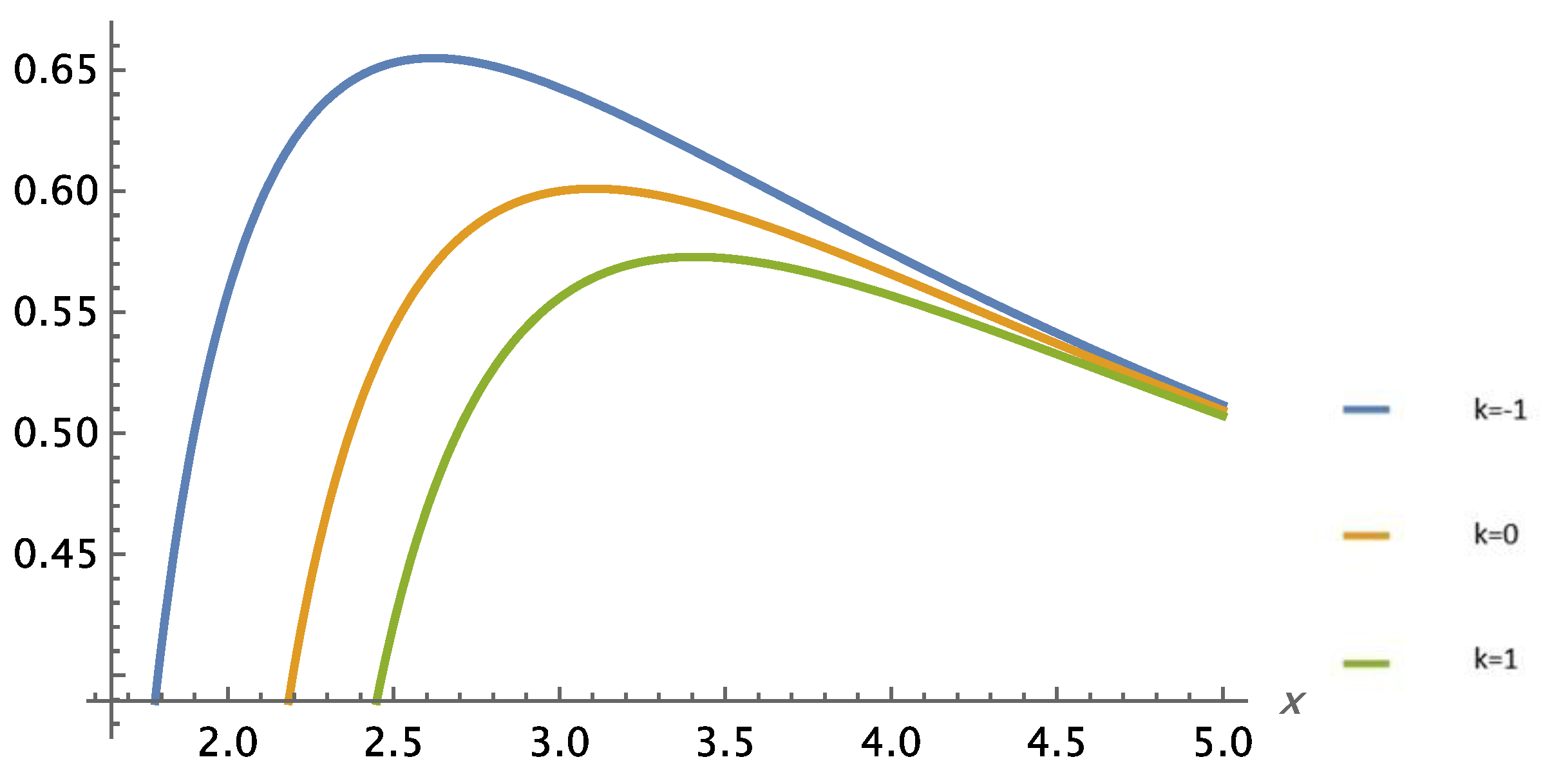
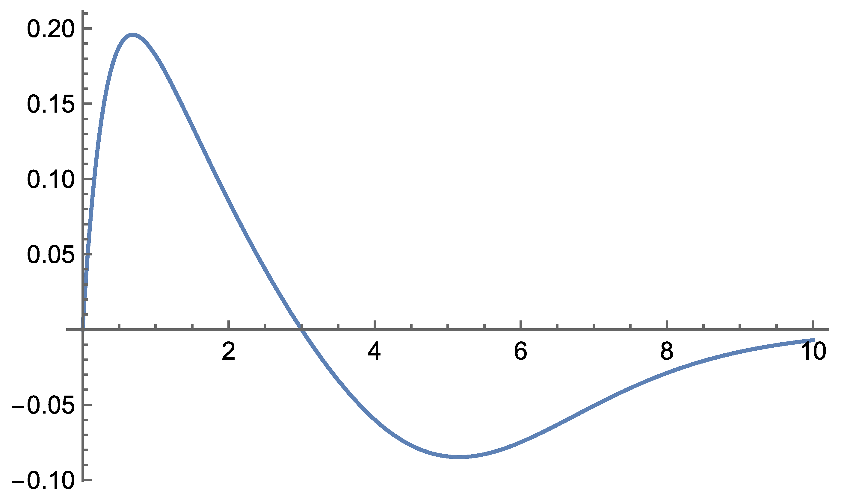
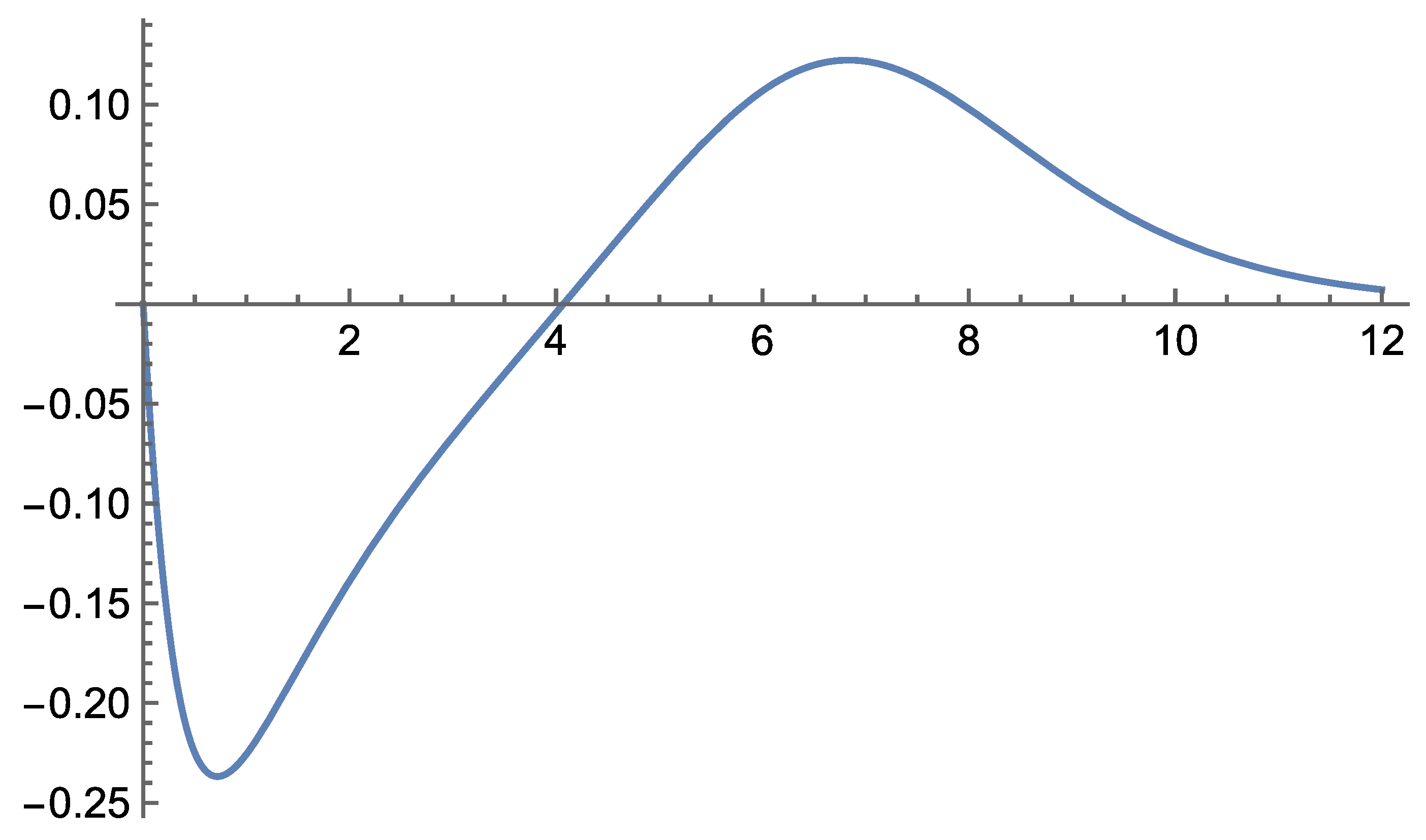
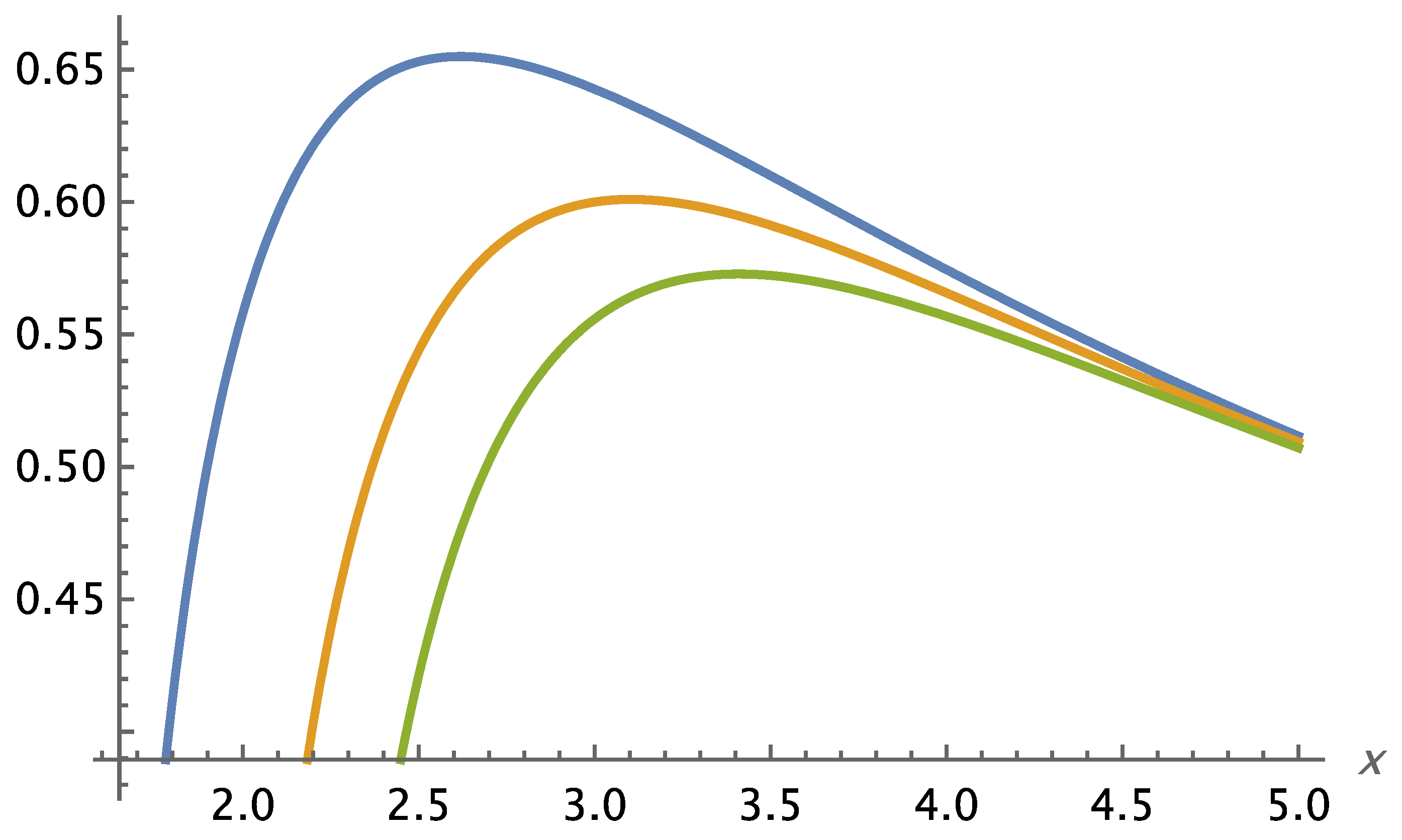
Figures 1.1, 1.2 and 1.3 plot the rotation speed of stars as a function of their distance from the center of galaxies and of galaxies as a function of their distance from the center of galaxy clusters (refer to Figures 4.20, 4.21 and 4.22). The rest mass distribution of the galaxy or galaxy cluster in space has not been taken into account in these graphs. The parameter is proportional to the distance from the mass of the galaxy or galaxy cluster. The parameter is a constant. The parameter is a constant of integration obtained from the solution of the differential equation that gives the gravitational interaction. The symbolism we follow is given in Chapter 4. Graphs 1.1, 1.2, 1.3 have already been recorded in a large number of galaxies, in which the velocity of the stars as a function of their distance from the galactic center has been measured (refer to [31], Section 1.8, Figure 1.7). The predicted rotation velocities as a function of the distance from the mass are completely different from the corresponding predictions of Newtonian gravity and General Relativity. It is the observational data that has led twentieth century Theories of Gravity to the hypothesis of Dark Matter. We expect that taking into account the spatial distribution of galaxy matter, we will have full agreement between theory and observational data [32,33,34,35,36,37,38,39,40,41,42,43,44,45,46,47,48].
Figure 1.1.
Interaction IV. The graph of the function , if , for small values of . Source: Figure by author.
Figure 1.1.
Interaction IV. The graph of the function , if , for small values of . Source: Figure by author.
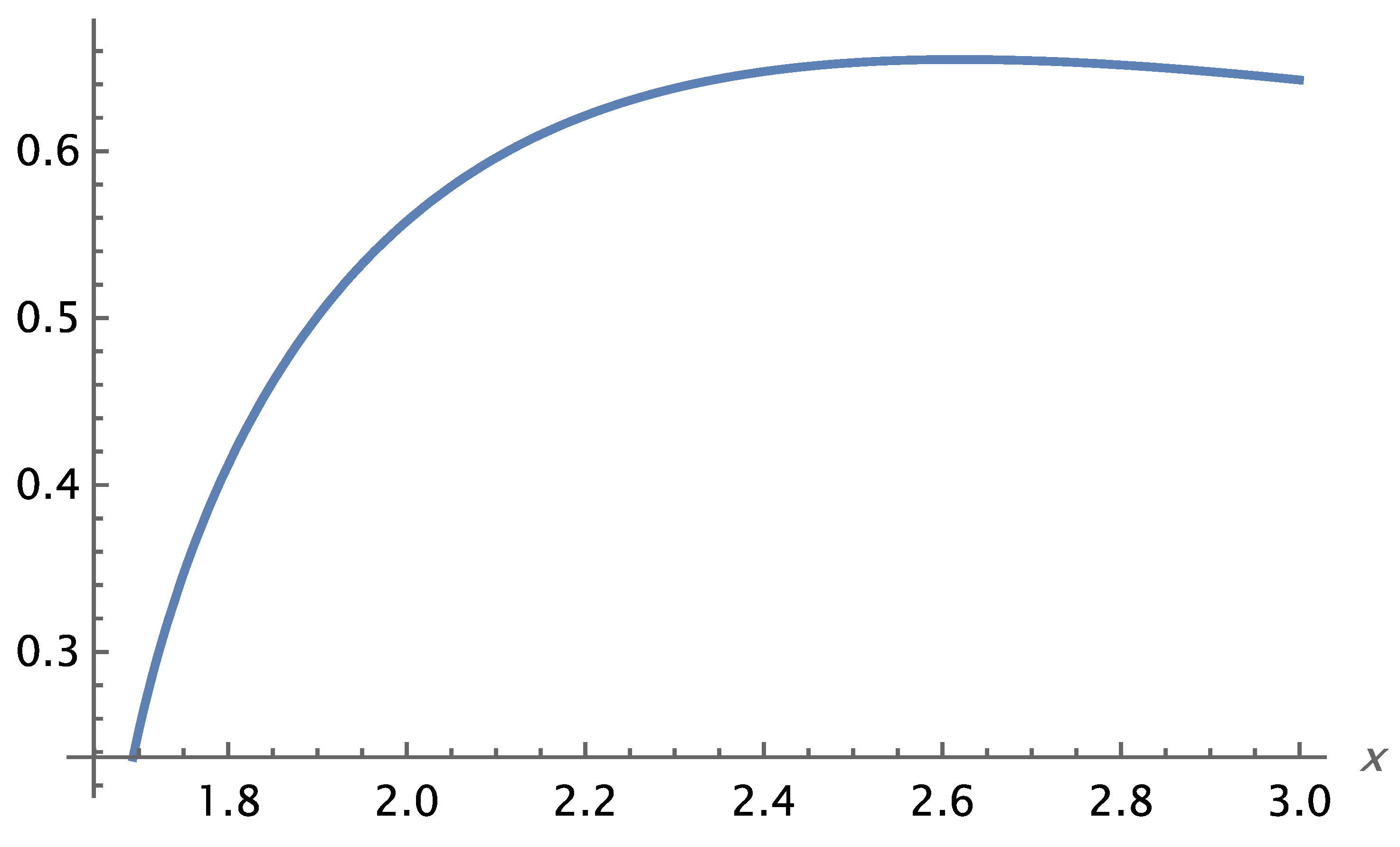
Figure 1.2.
Interaction IV. The graph of the function , if , for large values of . Source: Figure by author.
Figure 1.2.
Interaction IV. The graph of the function , if , for large values of . Source: Figure by author.
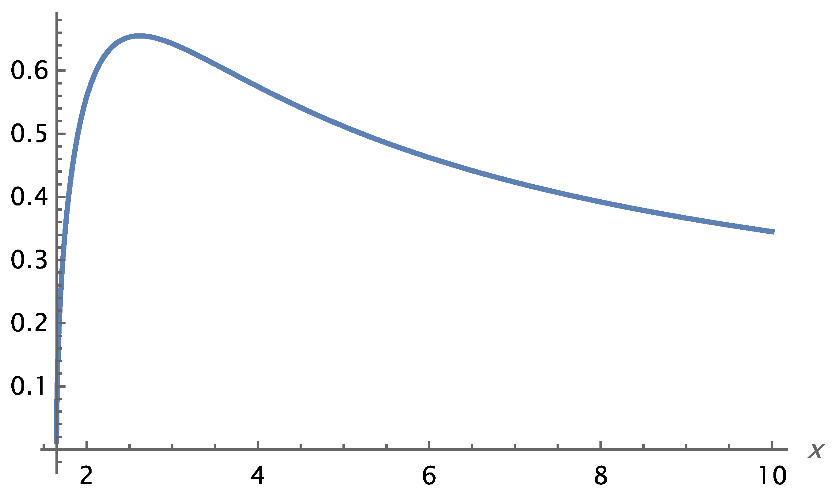
Figure 1.3.
Interaction IV. The graph of the function if , and . Source: Figure by author.
Interaction I predicts the same light deflection angle as General Relativity (GR),
General Relativity provides a precise prediction for the precession of the perihelion of planetary orbits, a phenomenon confirmed with high accuracy in the case of Mercury,
The Self-Variation Theory (Interaction I, ) also yields a corresponding prediction for the perihelion precession,
is a parametric constant introduced into the mass interaction equations of the Self-Variation Theory. When is set equal to , Self-Variation Theory reproduces the same expression as General Relativity for the perihelion precession of planetary orbits. It also predicts the Shapiro time delay,
For weak gravitational fields, such as that of the Sun, the deviation from the General Relativistic Shapiro delay,
predicted by the SVT potential is negligible. However, in the presence of stronger gravitational sources—such as neutron stars or black holes—the correction becomes increasingly significant and may be observationally detectable. The notation we follow in these Equations is given in Chapter 4.
In Chapter 5, we explore the cosmological implications of the self-variation principle. According to the theory, the rest mass and electric charge of a particle (more generally, its self-varying charge) appear smaller in cosmological-scale observations than their corresponding values measured in the laboratory on Earth. This has significant consequences for all physical phenomena in distant astronomical objects that depend on these fundamental quantities. These effects are imprinted in observational cosmological data. One prominent manifestation is the redshift of distant astronomical sources.
Many fundamental quantities in astrophysics depend on redshift. As a function of redshift, we compute: the electron mass (and more generally, the masses of fundamental particles), the ionization energy and the degree of ionization of atoms, the Thomson and Klein–Nishina scattering coefficients, the position–momentum uncertainty and the Bohr radius, as well as the energy released in nuclear reactions and hydrogen fusion.
Observational data indicate that the rate of increase of the electron’s charge (in absolute value) is significantly slower than the rate of increase of rest mass. This empirical result is in agreement with the theoretical prediction presented in Section 2.3, where a different growth rate for mass and charge was established as a consequence of self-variation.
One of the more striking implications is that, due to the self-variation of rest mass, gravity does not have cosmological-scale consequences: it is neither responsible for the expansion nor for any potential collapse of the universe. Gravitational effects are instead confined to smaller-scale structures, such as galaxies and clusters.
In Section 5.10, we compare the Standard Cosmological Model (SCM) with the predictions of Self-Variation Theory at cosmological scales. We highlight the reasons why the SCM has been compelled to adopt a series of auxiliary assumptions (e.g. dark energy, inflation, etc.) to align itself with observational data. However, certain observations—such as the two inconsistent measured values of the Hubble constant—currently lack a plausible explanation within the SCM framework.
By contrast, the origin and evolution of the universe as described by the Self-Variation Theory shows remarkable agreement with cosmological observations, offering a coherent and natural explanation for phenomena that remain puzzling under the standard model.
Fundamental quantities of astrophysics depend on redshift. We calculate as a function of the redshift the mass of the electron and in general the mass of the fundamental particles, the negative energy of spacetime, the ionization energy and the degree of ionization of the atoms, the Thomson and Klein-Nishina scattering coefficients, the position-momentum uncertainty and the Bohr radius , and the energy produced in nuclear reactions and hydrogen fusion. We give these parameters as a function of redshift ;
(refer to Equations are the (5.27), (5.46), (5.36), (5.38), (5.33), (5.40), (5.42) and (5.28)). The notation we follow in these equations is given in Chapter 5. Through these Equations we can follow the evolution of the universe, from its initial form to the most recent one, as we observe it today in the region of our galaxy. Many of the implications of these Equations are introduced into the Standard Cosmological Model as assumptions in order for the Model to agree with the cosmological data. However, the different evolution of the universe and the different prediction of the early universe by the Standard Cosmological Model, compared to the corresponding predictions of these Equations, leads the Standard Cosmological Model to an impasse. We give the predictions of the Self-Variation Theory in the very early universe, for observations at a large distance , theoretically if (refer to Section 5.11). For the rest mass of the particles and the rest energy in the surrounding spacetime (refer to limit (5.23), , and Equations (5.45) and (5.46)) we have
The Vacuum State is predicted as the beginning of the universe. The total mass / energy of the universe asymptotically tends to zero or is zero. Taking into account the conservation of energy-momentum we conclude that the universe, as a whole, is permanently in the Vacuum State (in the sense that its total energy content tends to zero or is equal to zero), at every moment in time, in all phases of its evolution. Therefore, on a cosmological scale the universe is predicted to be flat. From equation
it follows that at the beginning of the universe all its points communicated with each other (refer to Equations (5.41) and (5.43)). The horizon problem does not exist in the Self-Variation Cosmological Model. The Self-Variation Theory Equations on the cosmological scale predict that the universe may be much older and much larger in size than the Standard Cosmological Model predicts. None of the Equations of the Theory puts any restriction, any limit, on the values that the redshift can take. Going back in time, while the Standard Cosmological Model converges at one point, at the Big Bang, the Self-Variation Cosmological Model diverges, predicting an early universe of large dimensions.
In Section 5.10 we compare the Standard Cosmological Model with the predictions of Self-Variation Theory on the cosmological scale [8], [31,32,33,34,35,36,37,38,39,40,41,42,43,44,45,46,47,48,49,50,51,52,53,54,55,56,57,58,59,60,61,62,63,64,65,66,67,68,69,70,71,72,73]. The reasons why the Standard Cosmological Model has been forced into a series of assumptions to come to terms with the cosmological data are highlighted. However, there are now data, such as the two measured values of Hubble's constant, for which there is no plausible hypothesis that could bring them into agreement with the model. The origin and evolution of the universe as predicted by the Self-Variation Theory presents a remarkable compatibility with the cosmological data.
In Chapter 6 we study the wave resulting from the propagation of self-variation as a perturbation in 4-dimensional spacetime. We calculate the wave function and apply it to the hydrogen and muon atoms. In the context of Self-Variation Theory, the time-independent Schrödinger Equation describes the self-variation of electric charge at the atomic scale.
From 1901 when Planck solved the problem of electromagnetic blackbody radiation [74] until now, leading physicists have brought quantum mechanics to the level we know it today [75,76,77,78,79,80,81,82,83]. The use of quantum mechanical operators gives accurate results in all areas of physics in which it is applied. However, we do not know their physical content, which physical process or mechanism of nature they express. Self-Variation Theory relates the operators of quantum mechanics to self-variation. We prove that the operators of quantum mechanics express the compatibility of the laws of physics with the self-variation of material particles. This is one of the main conclusions of Self-Variation Theory (refer to Section 6.4). The self-variation of material particles explains quantum phenomena.
We study the interaction of electric charges as an exchange of "information". Through the self-variation potential, information is transferred from the charge-source of the electromagnetic field to infinity. We briefly present the consequences of electric charge self-variation in this information.
The exchange of signals at velocity , between two observers is not just an assumption we can make to derive Lorentz-Einstein transformations, but a physical reality. As a consequence of self-variation, particles continuously exchange energy-momentum, moving with velocity in flat spacetime. The Self-Variation Theory confirms the correctness of Special Relativity. We have a case of flat spacetime in the electromagnetic interaction, which we study in Chapter 3. As a consequence of self-variation, the energy-momentum exchange between particles takes place continuously, without interruption and in curved spacetime, but with a speed different from , . Cases of curved spacetime are studied in Chapter 4. One of these cases concerns the gravitational interaction.
The Self-Variation Theory gives a triple digit number of new, hitherto unknown final equations in all areas of physics. Despite the large number of equations it gives, the Theory is based on three principles. The principle of conservation of energy-momentum has been confirmed in an exceptionally large number of experiments and is now considered a law of physics. The definition of rest mass used in the mathematical formalism of the Theory is an obvious extension to the curved spacetime of rest mass as given by the Lorentz-Einstein transformations in Special Relativity. The new principle that the Theory introduces into the theoretical background of physics is that of self-variation. From the investigation of its consequences thus far, it appears that this principle brings theory into agreement with experiment and observational data, at all distance scales. A large part of this investigation is the content of this book.
2. Self-Variation in the Spacetime of Special Relativity. The Internal Symmetry Theorem
In this Chapter we study the generalized particle, as we defined it in the previous Chapter, in the flat 4-dimensional spacetime of Special Relativity. This study is fundamental, since it highlights the basic consequences of the self-variation of material particles. In the last Section of the Chapter we do the corresponding study in N-dimensional curved spacetime.
The main conclusion of the Chapter is the Internal Symmetry Theorem. This Theorem gives the rest mass and in general the charge of a particle as a function of spacetime. It also gives the relation of the energy-momentum and rest mass of a particle to the energy-momentum and rest mass in the surrounding spacetime of the particle. If the particle is charged, the Theorem gives a distribution of charge in the surrounding spacetime of the particle.
The Internal Symmetry Theorem justifies the so far known cosmological data in a flat and static universe. The analytical justification of the cosmological data is done in Chapter 5.
2.1. The Basic Equations of the Theory in Flat 4-Dimensional Spacetime
In flat spacetime there is no distinction between covariant and contravariant vectors. Thus, in the flat 4-dimensional spacetime (Minkowski spacetime) of Special Relativity [17,18,19,20,21], Equations (1.3) - (1.6) and (1.8) - (1.10) take the form,
, (2.1)
, (2.2)
, (2.3)
, (2.4)
, (2.5)
, (2.6)
(2.7)
respectively.
We consider an inertial frame of reference moving with velocity with respect to another inertial frame of reference , with their origins and coinciding at . With this symbolism the Lorentz-Einstein transformations have the following form,
(2.8)
, (2.9)
where .
From these transformations and Equation (1.15) (refer to Appendix A) we get the following equations,
(2.10)
and transformations,
(2.11)
, (2.12)
. (2.13)
It follows from our study that as we move from one frame of reference to another through Lorentz-Einstein transformations, we get equations that apply to the same frame of reference. They are Equations (2.10). Also, the vectors , ,
, (2.14)
(2.15)
are transformed like the electromagnetic field. The vectors and are parallel to the electric and magnetic fields respectively.
From Equations (1.15) and (2.10) we get,
. (2.16)
The determinant of the system of Equations (2.16) is given by the following equation,
as obtained after the necessary calculations. As a consequence of the principle of self-variation is , therefore the system of Equations (2.16) is non-homogeneous. Hence its determinant is non-zero,
. (2.17)
From the inequality (2.17) it follows that if for every , then . If then . One of the conclusions derived from the study we did is given by the following Internal Symmetry Theorem.
2.2. Internal Symmetry Theorem
In flat spacetime of special relativity the following applies.
A. If them .
B. If for each then the following applies.
1. The 4-vectors and are parallel,
. (2.18)
2. Exactly one of the following applies,
and (2.19)
or
, (2.20)
, (2.21)
, (2.22)
, (2.23)
(2.24)
where is a dimensionless constant.
Proof.
and with Equation (2.5) we get,
and with Equation (1.7) we get,
and with Equation (2.26) we get,
and after the calculations we get,
where is a dimensionless constant physical quantity.
and with Equation (1.2) we get,
and with Equation (2.19) we get,
and considering that it is we obtain,
and with the Equations
and (1.2) we get,
and with the Equation (2.28) we get,
and considering that it is we get,
and equivalently we get,
and with the Equation (1.7) we obtain,
A. A has already been proven, following Inequality (2.17). As a consequence of self-variation principle, and the system of Equations (2.16) is non-homogeneous.
B. 1. If for each , Equation (2.18) results from the system of Equations (2.16).
2. From Equation (2.18) we have and with Equation (1.7) we get and equivalently we obtain,
. (2.25)
If we have and . Then, from Equation (2.7) we obtain and from Equations (2.5), (2.6) we get and considering that and have opposite sign we obtain .
If , from Equation (2.25) we get,
. (2.26)
From Equations (2.5) and (1.2) we get,
. (2.27)
From Equation (2.27) we obtain,
From Equations (2.18) and (2.26) we obtain,
From this Equation and (2.6) we obtain,
Similarly, from Equations (2.26) and (2.5) we obtain,
The proof is completed by confirming the self-variation of the rest energy . For Equations (2.19) we have,
From Equations (2.21) and (2.22) we get,
. (2.28)
Then we have
The Internal Symmetry Theorem is generally valid for any self-variating charge, since in equation (1.1), the momentum of the particle is due to the charge .
Equations (2.19) predict a generalized particle with zero total rest mass, . In addition, the Equation applies. In this case, the Internal Symmetry Theorem does not give the relative position of the 4-vectors and .
For the generalized particle of Equations (2.20) - (2.24), the Internal Symmetry Theorem gives a remarkable set of information. From Equations (2.23) and (2.24) it follows that the 4-vectors , and are parallel in 4-dimensional spacetime. Equations (2.21) and (2.22) give the distribution of the total rest mass in and . Similarly, Equations (2.23) and (2.24) give the distribution of the total momentum along the axis. That is, we have energy-momentum and rest mass distribution in spacetime. This distribution is determined by the function . If in Equation (2.20) the distribution is periodic. In general, if the constant is not a real number, the distribution has wave characteristics. If it is a real number, the distribution is non-periodic.
From Equation (2.23) we have
. (2.29)
From Equations (2.29) and (1.7) we obtain,
. (2.30)
From equations (2.29) and (2.30) it follows that the Internal Symmetry Theorem gives the rates of change of the 4-vectors and .
The rest mass is considered "positive" and the rest energy "negative". Therefore, if , then the product
The function also depends on the 4-vector . If we have
Then, from Equation (2.7) we get
and
Then, from Equation (2.21) we obtain,
. (2.31)
As we will see in Chapter 5, Equation (2.31) accounts for the so far known cosmological facts.
2.3. Internal Symmetry Theorem for Charge
Rest mass may be due to self-variating charge. The charge contributes to the energy-momentum of a particle and therefore to its rest mass. We consider the 4-vector of the momentum due to the charge of the particle and the corresponding rest mass ,
Repeating the proof process of the Internal Symmetry Theorem we get,
Then, from Equation (1.1) we get
, (2.32)
where is a constant. Formulating the Internal Symmetry Theorem with respect to the charge , Equations (2.18) - (2.24) apply.
From Equation (2.32), if we get,
, (2.33)
Therefore, by substituting in Equations (2.18) - (2.31) we obtain the Internal Symmetry Theorem for the charge. The rest mass is due to the energy-momentum that the particle has due to the charge .
From the inequality
then the charge results in an increase in the rest mass of the particle.
then the charge results in a decrease in the rest mass of the particle. If the charge changes the rest mass of a material particle.
Equations (2.31) and (2.33) give the increase in rest mass and electric charge, as required by the self-variation principle, if . In the function , and therefore in the generalized particle, the concept of speed does not enter. Thus, the case where the generalized particle is stationary in a frame of reference can be expressed through the equation . However, equations (2.32) and (2.33) are also derived in a different way. In spherical coordinates , , , the equation (2.32) is written in the form
If the generalized particle is confined to a small space, or if the 3-dimensional vector , has a specific orientation in space, we again get equation (2.32),
. (2.34)
In this Equation the constant of Equation (2.31) has been replaced by the constant . Similarly, Equation (2.33) takes the form,
. (2.35)
For particles moving at low velocities, Equations (2.31) and (2.34) are practically equivalent since . Similarly, in Equations (2.33) and (2.35) it is , if the particles carrying the electric charge move with small velocities. In any case, Equations (2.31), (2.33) or (2.34), (2.35) hold when we consider the consequences of the time dependence of and .
2.4. The Internal Symmetry Theorem in Curved Spacetime
In N-dimensional curved spacetime [1,2,3,5,17], instead of Equation (2.5) the general Equation (1.8) applies,
From this Equation we get,
and with Equation (1.8) we obtain,
and with Equation (1.7) we obtain,
, (2.36)
where with we denote the covariant derivative with respect to . Now from Equations (1.17) and (1.7) we get and equivalently we get,
, (2.37)
where is the unit matrix. If , from Equation (2.37) we get
, (2.38)
where is the inverse of the matrix . Substituting the and , as derived from Equation (2.38) into Equation (2.36) we obtain a differential equation with unknown the elements of the matrix , that is, the functions . We solve the system of differential equations and get the functions . The solutions we obtain depend on the properties of the N-dimensional curved spacetime. The N-vector is constant.
A special case of the Theorem arises when the determinant of the matrix is equal to zero, . Assuming that , in order for the material particle to exist, the System of Equations (2.38) has a solution only if . Then, from Equation (1.10) we get , from Equation (1.7) , from Equations (1.8) and (1.9) and considering that and have opposite signs we get . Thus we get the case,
. (2.39)
These are Equations (2.19) which also arise in flat spacetime.
With the functions known, from the system of Equations (1.6) we get the relation of the momentums and . The momentums and enter the whole grid of the equations of the Self-Variation Theory. This has the consequence that the relationship between them, the Internal Symmetry Theorem, largely determines the structure of the generalized particle. We saw some of the consequences of the Theorem in the previous Sections of the Chapter, in the flat 4-dimensional spacetime of Special Relativity. One of these consequences concerns the correlation of the electromagnetic field with the functions , through Equations (2.14) and (2.15). Thus, one issue to investigate is the physical content of the functions in curved spacetime. Initially, these functions determine the relative position of N-vectors and in spacetime.
3. Electromagnetic Interaction
In this chapter, we present a new class of potentials—referred to as self-variation potentials—that are compatible with the self-variation principle and replace the traditional Liénard–Wiechert potentials in the surrounding spacetime of a point electric charge.
We study the electromagnetic field generated by a point electric charge undergoing arbitrary motion within an inertial frame of reference. This analysis leads to the substitution of the Liénard–Wiechert potentials by the self-variation potentials. Although both sets of potentials yield identical electromagnetic fields, they differ in their foundational principles and compatibility with physical laws.
Specifically:
The self-variation potentials are fully compatible with both the Lorentz–Einstein transformations and the self-variation principle.
The Liénard–Wiechert potentials, while compatible with the Lorentz–Einstein transformations, are not compatible with the self-variation principle when considered in the surrounding spacetime of a point charge.
Maxwell’s equations, as is well-known, are compatible with Lorentz invariance. In this chapter, we demonstrate that they are also compatible with the self-variation principle. Therefore, the fundamental laws of physics can be extended to incorporate self-variation.
Let us denote:
By , the set of equations compatible with Lorentz–Einstein transformations, and by , the set of equations compatible with the self-variation of electric charge, then we have: .
This means that Self-Variation Theory introduces additional constraints on the laws of physics beyond those imposed by Special Relativity.
In this chapter, we perform precise calculations to determine the consequences of self-variation in the spacetime surrounding a point charge . One key result is that an effective distribution of opposite electric charge appears in the surrounding spacetime due to self-variation. We compute both the electric charge density and the current density associated with this effect.
Furthermore, a geometric consequence of self-variation is established through the Orbit Representation Theorem. For each spatial direction, the trajectory (orbit) of the charge is mapped to a corresponding curve in the surrounding spacetime. The theorem relates the tangent vector, curvature, and torsion of these two curves, establishing a deep geometric link between the charge's motion and the structure of the surrounding spacetime.
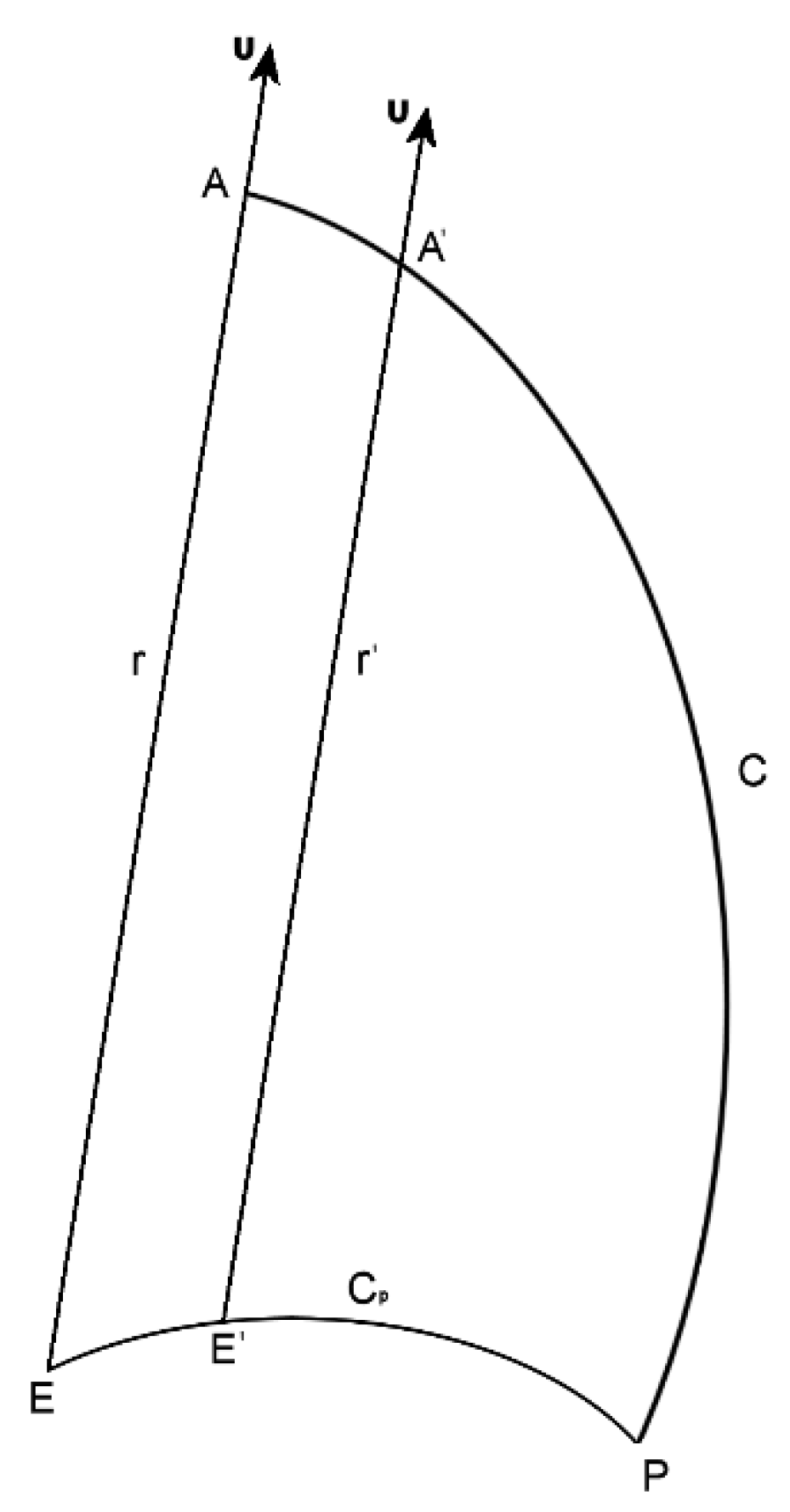
3.1. A Randomly Moving Electric Point Charge
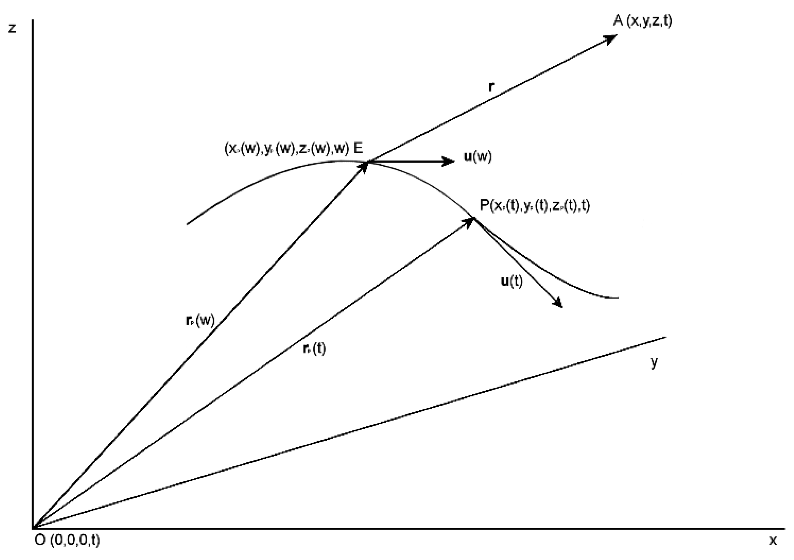
We consider an electric point charge moving randomly in an inertial frame of reference . We assume that the electromagnetic field propagates with speed , where is the speed of light in vacuum. As a consequence of self-variation, at time , when is at point , it acts on the fixed point with the value it had at point , at the retarded time . We use the following symbolism, , , , , , , ,
where . The index in the coordinates , , indicates the position of the point particle carrying the charge , at the corresponding moment in time or . At point we denote the velocity and the acceleration of , as in Figure 3.1.
With this symbolism we have,
, (3.1)
, (3.2)
, (3.3)
. (3.4)
The velocity of the at point is,
. (3.5)
Figure 3.1.
A randomly moving electric point charge . Source: Figure by author.
3.2. Auxiliary Equations
We prove the following list of equations that we will use next to simplify the mathematical calculations we do in this Chapter. From Equation (3.2) we have
. (3.6)
From Equations (3.3) and (3.6) we obtain,
. (3.7)
Starting again from Equation (3.2) we obtain,
. (3.8)
From Equations (3.3) and (3.8) we obtain,
. (3.9)
From Equation (3.1) we have
. (3.10)
From Equation (3.4) we have
. (3.11)
From Equation (3.4) we have
Working similarly, we finally obtain,
, (3.12)
where and .
Now we have,
. (3.13)
Working similarly we obtain,
. (3.14)
If a physical quantity is defined at the point , then we have,
. (3.15)
Similarly, from Equation (3.9) we obtain,
. (3.16)
From Equations (3.15) and (3.16) we obtain,
. (3.17)
As a consequence of self-variation, at time the electric charge acts at point with the value it has at point . Therefore, and from Equations (3.15), (3.16) and (3.17) For we obtain,
, (3.18)
, (3.19)
. (3.20)
We now consider the acceleration vector of at the moment located at point ,
. (3.21)
Applying equations (3.15) and (3.16) for the velocity components we obtain,
, (3.22)
, (3.23)
where and . Applying Equations (3.15) and (3.16) for the velocity components we obtain,
, (3.24)
, (3.25)
where .
Using the previous Equations we obtain the following equations,
, (3.26)
, (3.27)
, (3.28)
, (3.29)
after the necessary calculations.
The auxiliary equations simplify the analytical proofs we do in the next Sections of the Chapter. We also use these Equations in the calculations we do in Appendix B.
3.3. Liénard-Wiechert Potentials
With the notation we follow, the Liénard-Wiechert [9,10,11,12,13,14], [22,23,24,25] scalar-vector potential pair is given by the equations,
, (3.30)
, (3.31)
where is the permittivity of free space. The electric field and the magnetic field at point are given by the pair of the scalar potential and the vector potential respectively, through equations
, (3.32)
. (3.33)
Through Equations (3.30), (3.31) and (3.32), (3.33) the Liénard-Wiechert potentials give the following equations for the electromagnetic field at point ,
, (3.34)
. (3.35)
The first terms in the second members of Equations (3.34), (3.35) give the electromagnetic field accompanying the electric charge in its movement, and the second terms the electromagnetic radiation.
3.4. Self-Variation Potentials
As a consequence of self-variation, the electromagnetic potential splits into two pairs of potentials [7,30]. One pair,
(3.36)
gives the electromagnetic field that accompanies the electric charge in its motion,
. (3.37)
The other pair,
(3.38)
gives the electromagnetic radiation,
. (3.39)
From (3.37) and (3.39) we get Equations (3.34). The Liénard-Wiechert and self-variation potentials give the same equations for the electromagnetic field strength. From the potentials (3.36) we prove the first of Equations (3.37). Similarly, the proof of the second is done, as well as the proof of Equations (3.39) from the potentials (3.38).
Proof.
and equivalently we get,
and equivalently we get,
and equivalently we obtain,
and equivalently we get,
and equivalently we get,
and equivalently we get,
and equivalently we get,
and equivalently we obtain,
From Equation (3.32) and (3.36) we have,
. (3.40)
and with Equation (3.20) we get,
(3.41)
and equivalently we get,
. (3.42)
From Equation (3.17) if we get,
. (3.43)
From Equations (3.42) and (3.43) we get,
. (3.44)
From Equations (3.8) and (3.10) we get,
. (3.45)
From Equations (3.26) and (3.27) we get,
. (3.46)
From Equations (3.44) and (3.34), (3.45), (3.11), (3.4) we get,
In the proof we followed, the transition from Equation (3.40) to (3.41) was made as a consequence of Equation (3.20). This Equation expresses the self-variation of the electric charge . If we assume that the charge does not self-variate, from the potentials (3.36) we directly obtain Equation (3.41). The self-variation potentials give the same electromagnetic field whether we consider the electric charge to vary according to the self-variation principle or to be constant.
Liénard-Wiechert potentials and self-variation potentials give the same electromagnetic field. However, self-variation potentials are compatible with Lorentz-Einstein transformations and, obviously, with the self-variation principle. The Liénard-Wiechert potentials are compatible with Lorentz-Einstein transformations, but it are not compatible with the self-variation principle, in the surrounding spacetime of a point electric charge. If we denote by the set of equations that are compatible with the Lorentz-Einstein transformations and by the set of equations that are compatible with the self-variation of the electric charge then it is . Regarding the mathematical formalism of the laws of physics, the Self-Variation Theory imposes additional constraints than those imposed by Special Relativity.
Applying Maxwell's Equations for the electromagnetic field of Equations (3.34), (3.35) it follows that at point there is an electric charge, as a consequence of self-variation, with density and current density ,
. (3.47)
As a consequence of self-variation, in the surrounding spacetime of there is an electric charge of opposite sign (), as follows from Equations (3.47). We prove the first of Equations (3.47). Similarly, the proof of the second Equation is made (refer to Appendix B).
Proof.
and with Equation (3.50) we get,
and equivalently we get,
and with Equation (3.19) we get,
and equivalently we get,
and equivalently we get,
and equivalently we obtain,
and with Equation (3.18) we obtain,
From Maxwell's first law we have,
. (3.48)
We write equation (3.34) in the form,
. (3.49)
If we ignore self-variation and consider constant, at point there is no electric charge. Thus from Equations (3.48) and (3.49) we get,
. (3.50)
Equation (3.50) is also proved using the auxiliary Equations (3.6) - (3.29). From Equations (3.48) and (3.49) we get,
Therefore, the charge density at point is given by the equation,
.
Furthermore, electromagnetic radiation does not contribute to the electric charge of spacetime.
We now prove the continuity equation at point ,
. (3.51)
Proof.
and equivalently we get,
and with Equation (3.13) we get,
and equivalently we get,
From Equation (3.47) we have,
. (3.52)
The charge and the velocity are defined at point . Then, from the first of Equations (3.47) we get the density in the form,
. (3.53)
From Equations (3.52) and (3.53) we get,
. (3.54)
From Equations (3.15) and (3.16) we get,
. (3.55)
From Equations (3.6) and (3.8) we get,
. (3.56)
From Equations (3.26) and (3.27) we get,
. (3.57)
From Equations (3.54) and (3.55), (3.56), (3.57) we get,
The continuity equation expresses the conservation of charge distributed in spacetime. This conservation of charge is equivalently expressed through the equation,
. (3.58)
Considering the independence of velocity [17] from velocity at point , the volume in Equation (3.58) is a sphere centered at point and radius . Equation (3.58) can also be proved independently of the continuity equation, by using the auxiliary Equations (3.6) – (3.29) (refer to Appendix C). From Equation (3.58) it follows that two observers in points and , for the same particle (carrying the charge ) measure a value for their own particle and the value with which the particle of the other acts in theirs.
To understand the physical content of Equation (3.58), let us assume that the particle at point is an electron carrying a charge . In the time interval from to , , the increase in is balanced by the charge of spacetime, which is distributed over the sphere with center and radius . The charge of spacetime is due to the electromagnetic field that accompanies the electron. If we assume that this field exists in every case, the increase of is continuous. We now assume that the electron is stationary () at point . The increase of to over time is given by the equation (2.33). Therefore, the constant rest mass determines the increase in over time.
Self-variation potentials are compatible with Lorentz-Einstein transformations and, obviously, with the self-variation principle. The Liénard-Wiechert potentials were published seven years before the publication of Special Relativity by Einstein [13]. After the formulation of Special Relativity it was shown that they are compatible with Lorentz-Einstein transformations. From Equations (3.30), (3.31) it is proven that the Liénard-Wiechert potentials are not compatible with the self-variation principle. For them to be compatible, the self-variation principle should have given the equation
(3.59)
and not (3.20),
In the surrounding spacetime of , Equation (3.20) holds. If Equation (3.59) holds, the Liénard-Wiechert potentials are compatible with self-variation. We study this case in Chapter 6.
3.5. Orbit Representation Theorem
In this Section we prove the Orbit Representation Theorem. In Figure 3.2, the point electric charge is at point . By we denote the orbit in which moved in the past time, until it is at point .
Figure 3.2.
Curves and in the surrounding spacetime of a randomly moving point electric charge . Source: Figure by author.
Figure 3.2.
Curves and in the surrounding spacetime of a randomly moving point electric charge . Source: Figure by author.
The Frenet equations,
, (3.60)
uniquely define a curve . denotes the tangent vector, the curvature vector, and the curvature and torsion respectively, the arc length of the curve , and .
We calculate the tangent vector , the curvature and the torsion of the curve at the point . First we calculate the arc length . We have (refer to Figure 3.1),
. (3.61)
If we have,
. (3.62)
The curvature vector is given by equation,
. (3.63)
Now we have,
. (3.64)
From Equations (3.63) and (3.64) we get,
. (3.65)
From Equation (3.65) we obtain,
. (3.66)
From Equations (3.65) and (3.66) we obtain,
. (3.67)
For the vector we have,
. (3.68)
From the third of Equations (3.60) we get
. (3.69)
Equations (3.62), (3.66), (3.69) give the tangent vector , curvature and torsion of the curve respectively.
For each direction the curve is mapped onto another curve in the surrounding spacetime of the point electric charge . This mapping is given by the following Theorem.
Orbit Representation Theorem
For each direction the following hold.
1. The mapping maps the orbit of point electric charge onto the curve in its surrounding spacetime,
. (3.70)
2. The mapping maps the curve onto the orbit ,
. (3.71)
Proof.
we get Equations (3.72), (3.73), (3.74), (3.75), (3.76) and (3.77). From Equations (3.72), (3.73), (3.74), (3.75), (3.76) and (3.77), by substituting
we get Equations (3.62), (3.65), (3.67), (3.68), (3.66) and (3.69).
In Figure 3.2, in the direction of the vector the curve is depicted in the curve . In Appendix D we calculate the elements of the C curve, as given below.
The tangent vector is given by the equation,
. (3.72)
The curvature vector is given by the equation,
. (3.73)
The vector is given by the equation,
, (3.74)
if .
The vector is given by the equation,
. (3.75)
The curvature is given by the equation,
. (3.76)
The torsion is given by the equation,
. (3.77)
From Equations (3.62), (3.65), (3.67), (3.68), (3.66) and (3.69), by substituting
With the proof of the Orbit Representation Theorem we have the main consequences of the self-variation in the surrounding spacetime of the point electric charge . The first consequence concerns the geometry of spacetime. For each direction in space, curve is depicted in curve . The second consequence concerns the existence of electric charge and electric current in spacetime. The charge density and current density in spacetime are given by Equations (3.47). As a consequence of self-variation, the charge affects both the geometry and the physical quantities contained in spacetime.
We now apply the Orbit Representation Theorem to a particular case. If
from Equations (3.34) and (3.35) it follows that the electromagnetic radiation is set to zero in the surrounding spacetime of the point electric charge . This acceleration also has a second consequence on the surrounding spacetime of the point electric charge . From Equation (3.73) it follows that the curvature vector of is zeroed, . For the particular acceleration , the curve is a straight line. For the curve , the tangent vector, curvature and torsion are given by Equations (3.62), (3.66) and (3.69) respectively. The point particle carrying the charge moves in a curved orbit, with its representation in spacetime being straight.
3.6. The 4-Vectors and
In this Section we calculate the 4-vectors and . Then, through Equations (2.5), (2.26) and (2.7) we calculate the rest masses and . From Equation (3.18) and we get,
(3.78)
we obtain,
. (3.79)
For the 3-dimensional momentum , from Equations (3.19) and (1.1) we get,
. (3.80)
From Equations (3.79) and (3.80) we obtain,
. (3.81)
Equations (3.79) and (3.80) give the 4-vector , in the direction . From these Equations it follows that the 4-vector depends on the rate of change of charge . As a consequence of self-variation, this rate of change cannot be zero, . So the 4-vector also cannot be zeroed, .
From Equation (2.6) written in the form,
. (3.82)
Therefore the rest mass is equal to zero. This result is expected, due to the equation . If the electromagnetic interaction is due to a particle, then that particle has zero rest mass.
From Equations (3.79), (3.80) and (1.7) we get,
(3.83)
and
. (3.84)
Equations (3.83) and (3.84) give the 4-vector , in the direction .
In Section 2.3 we got the function from the function . In the electromagnetic interaction the momentum is a consequence of the self-variation of the charge . Therefore, in the electromagnetic interaction the function is determined by the self-variation of the charge . From Equations (3.83), (3.84) and (2.5) we get,
. (3.85)
Equation (3.85) gives the additional rest mass of the particle, which is due to the electric charge . The contribution of the electric charge to the rest mass of the particle is different for each direction .
There are two directions for which takes two special forms. These cases concern the relative position of the vectors and . If , then we have
, (3.86)
and Equation (3.85) becomes,
. (3.87)
From Equation (2.7) we have,
. (3.88)
If , then we have
, (3.89)
From Equation (3.89) we again get
and Equation (3.85) becomes,
. (3.90)
Equation (3.85) gives the factors that determine the contribution of the electric charge to the rest mass of an electrically charged particle. There are two directions
3.7. Electromagnetic Interaction Symmetries
In the flat spacetime of Special Relativity, the -functions give the relative position of the 4-vectors and (refer to Equation (2.16)). However, from the study we did in Chapter 2 it emerged that the -functions, , are related to the electromagnetic field. The vectors , of Equations (2.14) and (2.15),
, (3.91)
, (3.92)
where is a physical quantity invariant by Lorentz-Einstein transformations or a constant (with unit of Tesla). Now from Equations (3.91), (3.92) and (3.34), (3.35) we get the relationship of the electromagnetic field in the surrounding spacetime of a point electric charge with the physical quantities , ,
. (3.93)
From Equations (3.34) and (3.35) we get,
(3.94)
and with Equation (3.81) we obtain,
. (3.95)
From Equations (3.95) and (3.91), (3.92) we obtain the following equations,
. (3.96)
Taking into consideration the equations and (3.95), Equations (3.96) are written in the form,
, (3.97)
where , , , . From Equation (3.94) we get and with Equations (3.93) we obtain,
. (3.98)
Equations (3.97) and (3.98) give the symmetries of the electromagnetic interaction. Through Equation (1.7), from Equation (3.97) we obtain,
. (3.99)
From Equations (3.97) and (3.99) it follows that the electromagnetic interaction is not symmetric under the substitution . This asymmetry is a consequence of the self-variation principle. The principle is formulated by Equation (1.2) and not Equations (1.13), (1.14). In order for self-variation to exist the rest mass cannot be equal to zero, . Vice versa, the rest mass can be set to zero. In the electromagnetic interaction it is (refer to Equation (3.82)), resulting in the asymmetry of Equations (3.97) and (3.99).
From Equations (3.91) and (3.92) it follows that the Internal Symmetry Theorem (refer to Equations (2.19) – (2.24)) is valid when the electromagnetic field becomes zero, for every . The charge does not interact with any other charge, and the rate of change of the 4-vectors and is an internal matter of the generalized particle, as follows from Equations (2.29) and (2.30). In the context of Self-Variation Theory, this state is considered as the simplest state of the generalized particle and always occurs in flat spacetime.
3.8. Comparison Between Self-Variation Theory and Classical Electrodynamics: Convergences and Divergences
How Do the Convergences Arise?
The similarities between Self-Variation Theory (SVT) and classical electrodynamics (including Liénard-Wiechert potentials) stem from the fact that both are formulated within the framework of special relativity:
Lorentz Invariance: SVT operates fully within Minkowski spacetime and respects Lorentz transformations, just like classical electromagnetism.
Field Equivalence: Even though the potentials differ in form, the electric and magnetic fields (E, B) produced by SVT potentials are identical to those obtained via Liénard-Wiechert potentials.
Separation of Field Components: Both theories distinguish between near-field (non-radiative) and far-field (radiative) components associated with moving charges.
Consistency in Static vs. Self-Varying Charges: SVT predicts the same field structure whether the charge is constant or self-varying—highlighting a robustness in its field definition.
Divergence and Its Causes
The core divergences arise from SVT's introduction of a new physical principle: the self-variation of rest mass and charge. This leads to several key differences:
Source Dynamics: In SVT, the charge and mass of a particle are not fixed—they increase over time, leading to a continuous outflow of energy and momentum. In contrast, classical theory assumes fixed intrinsic properties for particles.
Origin of Radiation: In classical electrodynamics, radiation results strictly from acceleration. In SVT, energy-momentum radiation is a direct consequence of the self-variation principle, regardless of acceleration.
Distributed Charge-Mass Structure: SVT proposes that mass and charge are not purely point-like but have an evolving spatial distribution around the particle due to the self-variation process.
Foundational Principles: Classical electrodynamics is based on Maxwell's equations and conservation laws. SVT adds an entirely new foundational axiom—the self-variation principle—which redefines the role and nature of sources.
Potential Structure: The SVT potentials contain additional terms that account for self-variation effects, which are absent in Liénard-Wiechert potentials, even though both yield the same fields.
What Are the Implications of These Differences?
Physical Interpretation of Mass and Charge: SVT challenges the idea of invariant rest mass and charge, suggesting instead that these properties evolve dynamically.
Redshift and Cosmology: The theory potentially links mass evolution with cosmological redshift, proposing that particles' rest mass increases with proper time or distance—offering an alternative interpretation to standard cosmological models.
Experimental Predictions: Although the resulting fields match classical predictions under many conditions, SVT may lead to subtle deviations in radiation profiles, energy distributions, or long-range interactions, especially in high-precision regimes.
Field Source Duality: The distinction between constant and varying sources becomes less significant in SVT, which unifies them under a broader principle.
Conclusions
While Self-Variation Theory is constructed to be consistent with special relativity and yields the same observable electromagnetic fields as classical theory, it redefines the internal dynamics of field sources. The theory introduces a novel principle—that rest mass and charge self-vary—leading to a reinterpretation of the nature of particles, field generation, and radiation.
These theoretical divergences do not contradict experimental electrodynamics, but they enrich the conceptual foundation and may lead to new testable predictions, especially in contexts where the internal structure and evolution of sources become significant.
4. Gravitational Interaction
In this chapter, we formulate the gravitational field equations within the framework of the Self-Variation Theory. A central feature of Self-Variation Theory is that it describes both gravity and electromagnetism using a unified set of equations. These equations govern the fields generated by the rest mass and/or electric charge of a particle.
The core equation of the theory establishes a relationship among three fundamental physical quantities: the rest mass (or electric charge) of the source, its relative velocity with respect to the observer, and the propagation speed of the field as measured by the observer. These velocities are directly linked to the observed field potential and field strength.
Initial analytical results show that the theory remains consistent across the range of distance scales for which we have observational data. Notably, Self-Variation Theory predicts enhanced rotational velocities of stars in galaxies, as well as galaxies within galaxy clusters—phenomena typically attributed to dark matter.
According to the field equations derived in Self-Variation Theory, gravity behaves differently depending on the distance from the source mass: it is repulsive at very short ranges and becomes attractive beyond a certain critical distance.
Notably, the scope of these equations extends beyond the domains of gravity and electromagnetism. In the course of analyzing the fundamental equation of the Self-Variation Theory, it was found that rest mass participates in eight distinct interactions, which are organized into two groups. Each group comprises four interactions that exhibit common physical characteristics. Remarkably, the equations governing each of these interactions encapsulate an extensive amount of information, all of which originates from a single fundamental expression. This highlights the strongly unifying nature of the Self-Variation Theory.
For all eight interactions, we provide explicit expressions for the field propagation speed, potential, and strength as functions of the radial distance from a point-like rest mass. The corresponding field equations are defined both in the surrounding spacetime of the point mass and at the location of the mass itself.
Interaction I predicts the same light deflection angle as General Relativity, with Δϕ ≈ 1.75 arcseconds, when light passes at its minimum distance from the Sun. Within the framework of the Self-Variation Theory, a parametric constant is introduced into the mass interaction equations. When is set equal to , where is the speed of light in a vacuum, SVT reproduces the same expression as General Relativity for the perihelion precession of planetary orbits. It also predicts the Shapiro time delay, with a deviation that for the Sun is about seconds from the prediction of General Relativity.
4.1. Gravitational Potential
Through a series of mathematical calculations, the self-variation principle necessarily involves a modification of the electromagnetic potential, in the surrounding spacetime of a point electric charge [7,8,30]. For comparison the classical electromagnetic Liénard–Wiechert potentials are,
whereas the corresponding self-variation potentials are,
The difference lies in the potential
The self-variation potential associated with the gravitational interaction is derived in direct analogy with the corresponding electromagnetic case. Specifically, beginning with the equations that govern the electromagnetic self-variation potential, the gravitational analogues are obtained by applying the following substitutions:
Replace the electric charge with the rest mass of the source of the gravitational field, such that:
Through these substitutions, we obtain the expressions for the self-variation potentials corresponding to the gravitational interaction. These potentials mirror the form of their electromagnetic counterparts, but they are governed by mass distributions and gravitational field intensities instead of electric charges and electromagnetic fields,
, (4.1)
where , is the velocity of the rest mass relative to the observer, and , is the distance from the rest mass .
Deriving the gravitational potentials in this manner suggests the existence of a gravitational analog to the magnetic field (see Equations (3.30)–(3.33)). This field carries its own set of units, .
It is important to note that, in the limiting case where the propagation speed of the gravitational interaction υ tends to infinity (i.e., υ→∞), the resulting gravitational potential reduces to:
which corresponds precisely to the Newtonian gravitational potential
Analogously to its electromagnetic counterpart, Equation (4.1) describes the gravitational field generated by the rest mass of an individual particle. By extending this formulation to a continuous distribution of matter in spacetime, we obtain the corresponding gravitational field on a macroscopic scale. This macroscopic field emerges from the collective contribution of all mass elements and forms the basis for gravitational field theory in continuous media.
4.2. Potential, Propagation Speed, and Strength of the Gravitational Field Generated by a Stationary Point Mass
Equation (4.1) encapsulates the full structure of the self-variation potential for gravity, accounting for all possible interactions in which a given mass may participate. In this section, we consider the simplest physical configuration: a point mass at rest. This idealized scenario provides a clear baseline for understanding the gravitational field in the absence of motion or external influences.
Starting from Equations (1), and applying the appropriate assumptions for a stationary point mass, we obtain:
From this equation, and taking into account that the vectors and are parallel in the case of a stationary point mass, we deduce that the scalar potential,
. (4.2)
This result serves as the starting point for analyzing the static gravitational field, its strength as a function of distance, and the implications of a finite versus infinite propagation speed for gravitational interactions.
In the case of a stationary point mass, the strength of the gravitational field is given by the standard relation:
, (4.3)
where is the scalar gravitational potential and the radial distance from the mass. Furthermore, we have:
Combining the two expressions yields:
Multiplying both sides by , and recognizing that
we obtain:
, (4.4)
where is a constant of integration with units of , determined by boundary conditions or normalization of the potential. The sign in Equation (4.4) reflects the inclusion of a constant term
into the potential, either as an additive or subtractive contribution.
From Equations (4.2) and (4.3) we get
Combining this result with Equation (4.3), we derive the following system of equations, which governs the gravitational field generated by a stationary point mass:
(4.5)
The field strength is calculated from Equation (4.3).
We now introduce the variable transformation:
, (4.6)
into Equations (4.5). Under this change of variables, the system of Equations (4.5) can be rewritten in the following form:
(4.7)
This transformation simplifies the equations by reducing the number of physical parameters and rendering the system dimensionless, thereby facilitating both analytical and numerical analysis of the gravitational field. By applying the variable transformation introduced earlier, Equation (4.3) can be expressed in the following form:
. (4.8)
The system of differential equations (4.7) gives rise to eight distinct interactions involving mass. These interactions can be classified into two groups, depending on whether the exponential integral function appears in their analytical expressions. For each interaction, it is possible to compute the propagation velocity, the potential, and the field strength. A common feature of all interactions is their non-monotonic nature: none is purely attractive or purely repulsive across all distances. Instead, there exists a critical distance from the point mass at which the interaction changes character, transitioning either from repulsion to attraction or vice versa.
Interaction I
, (4.9)
, (4.10)
. (4.11)
Interaction II
, (4.12)
, (4.13)
. (4.14)
Interaction III
, (4.15)
, (4.16)
. (4.17)
Interaction IV
, (4.18)
, (4.19)
. (4.20)
The interactions of the first group do not exhibit singular behavior at the location of a point mass. Both the propagation velocity and the field strength vanish at this point, while the potential assumes a constant, non-zero value. Specifically, at a distance χ = 0 from the point mass, the potential for each of the four interactions in the first group is given by:
None of the interactions described by the potential (4.1) are strictly attractive or strictly repulsive. Instead, each interaction exhibits a critical transition at a specific distance () from the point mass, where the effective force changes sign—switching from repulsion to attraction or vice versa. For each of the four gravitational interaction models in the first group, this critical distance is determined by the solution of the following characteristic equations.
Interaction V
, (4.21)
. (4.22)
Interaction VI
, (4.23)
. (4.24)
Interaction VII
, (4.25)
. (4.26)
Interaction VIII
, (4.27)
. (4.28)
I–VIII pertain to mass interactions and are therefore not restricted solely to gravitational phenomena. They are applicable to all types of interactions in which mass plays a role.
4.3. Propagation Speed, Potential, and Field Strength Diagrams for Interactions I–IV
The value of the parameter determines the qualitative behavior of each interaction. This dependence is illustrated in the following diagrams. For interactions I–IV, we present plots of the functions
corresponding to selected values of the parameter .
Interaction I
Figure 4.1.
Interaction I. The function if . Source: Figure by author.
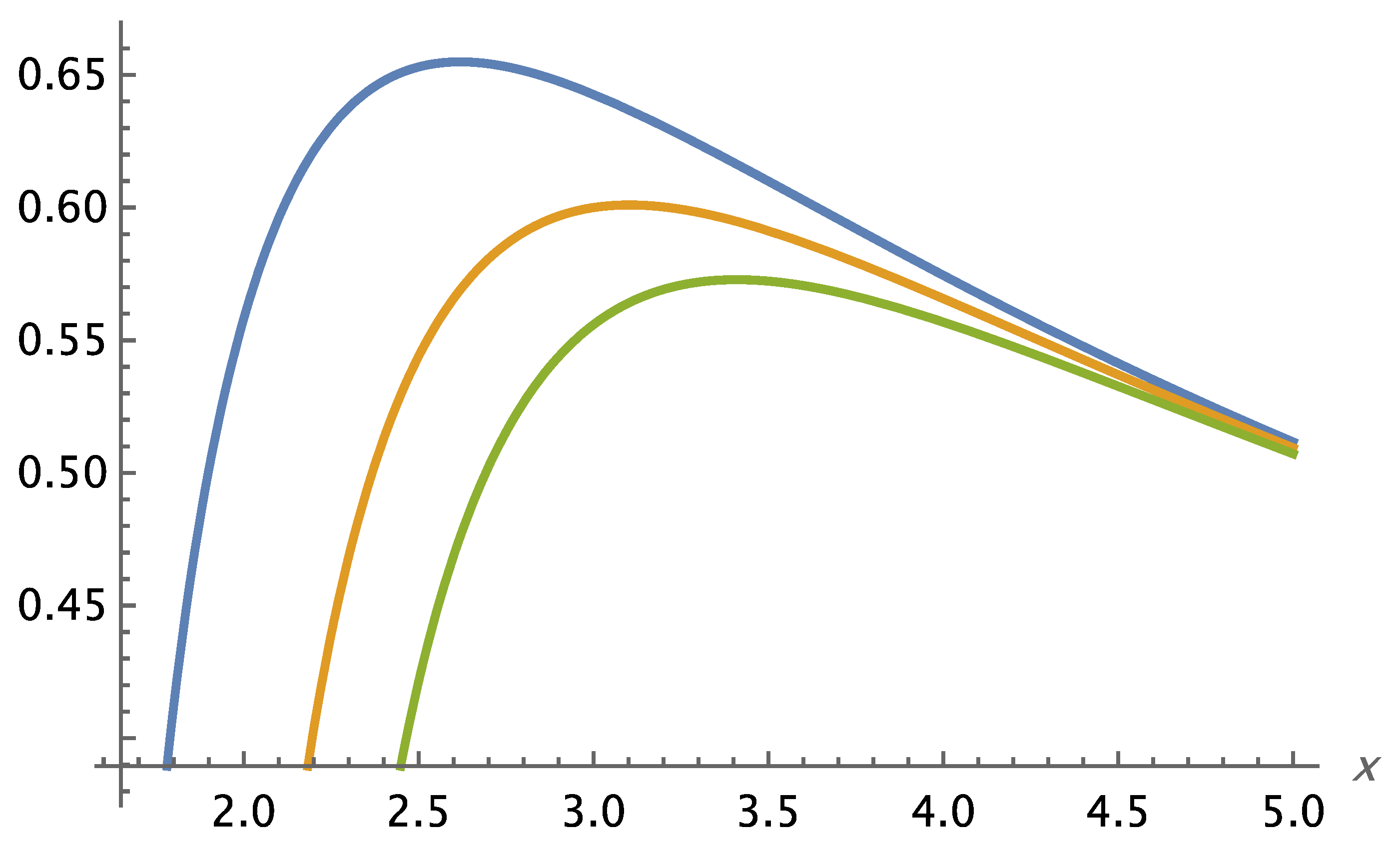
Figure 4.2.
Interaction I. The function if . Source: Figure by author.
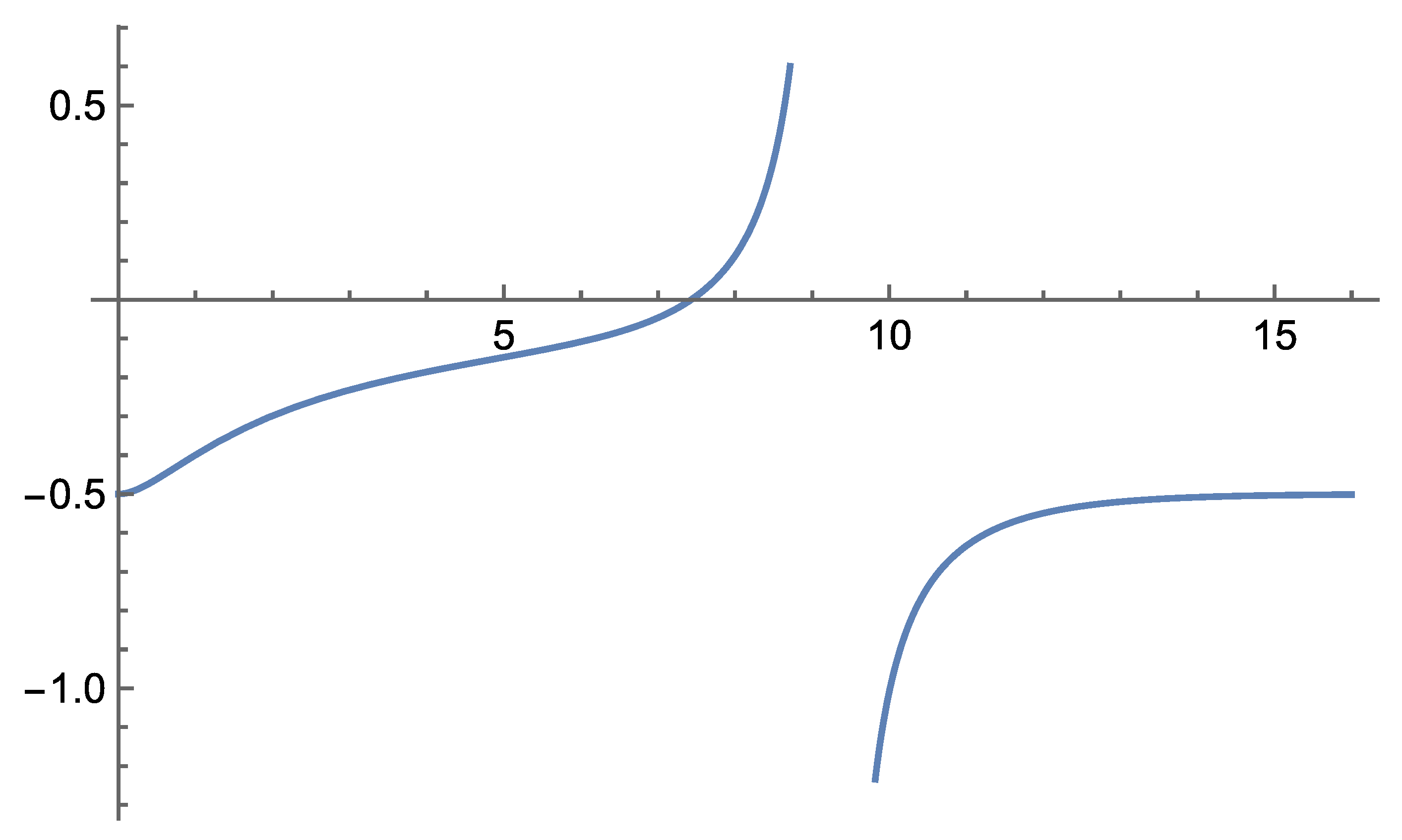
Figure 4.3.
Interaction I. The function if . Source: Figure by author.
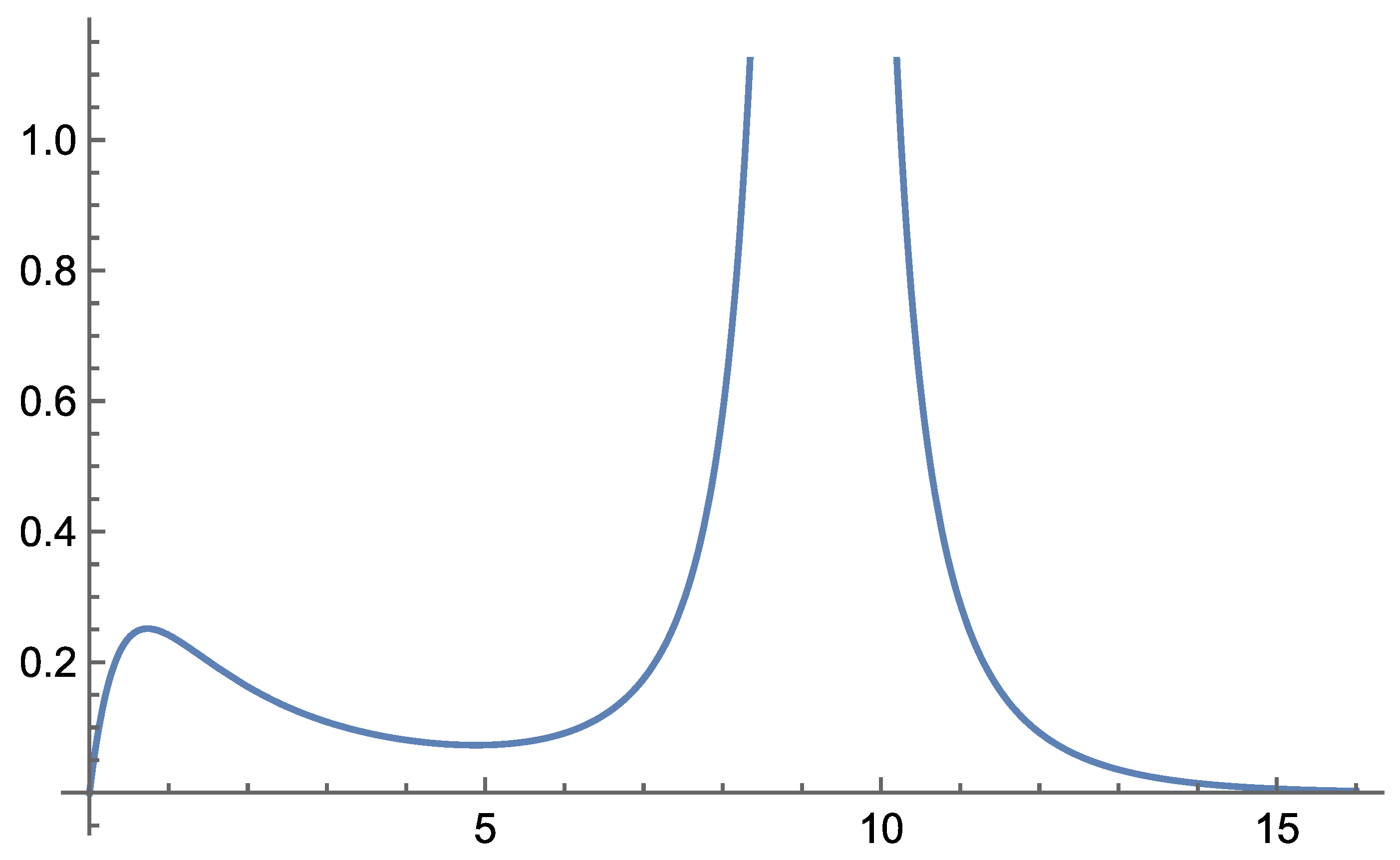
Figure 4.4.
Interaction I. The function if . Source: Figure by author.
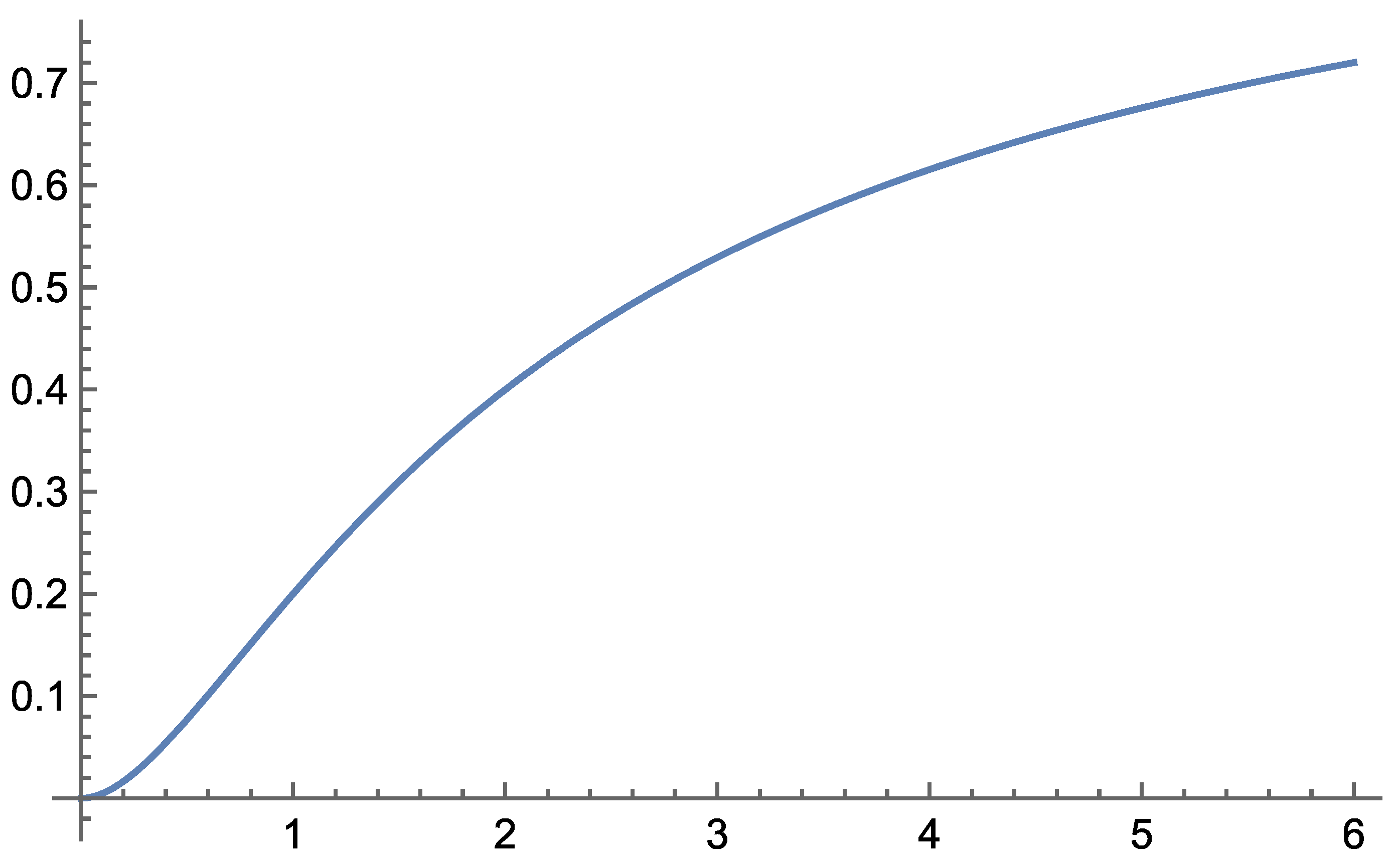
Figure 4.5.
Interaction I. The function if . Source: Figure by author.
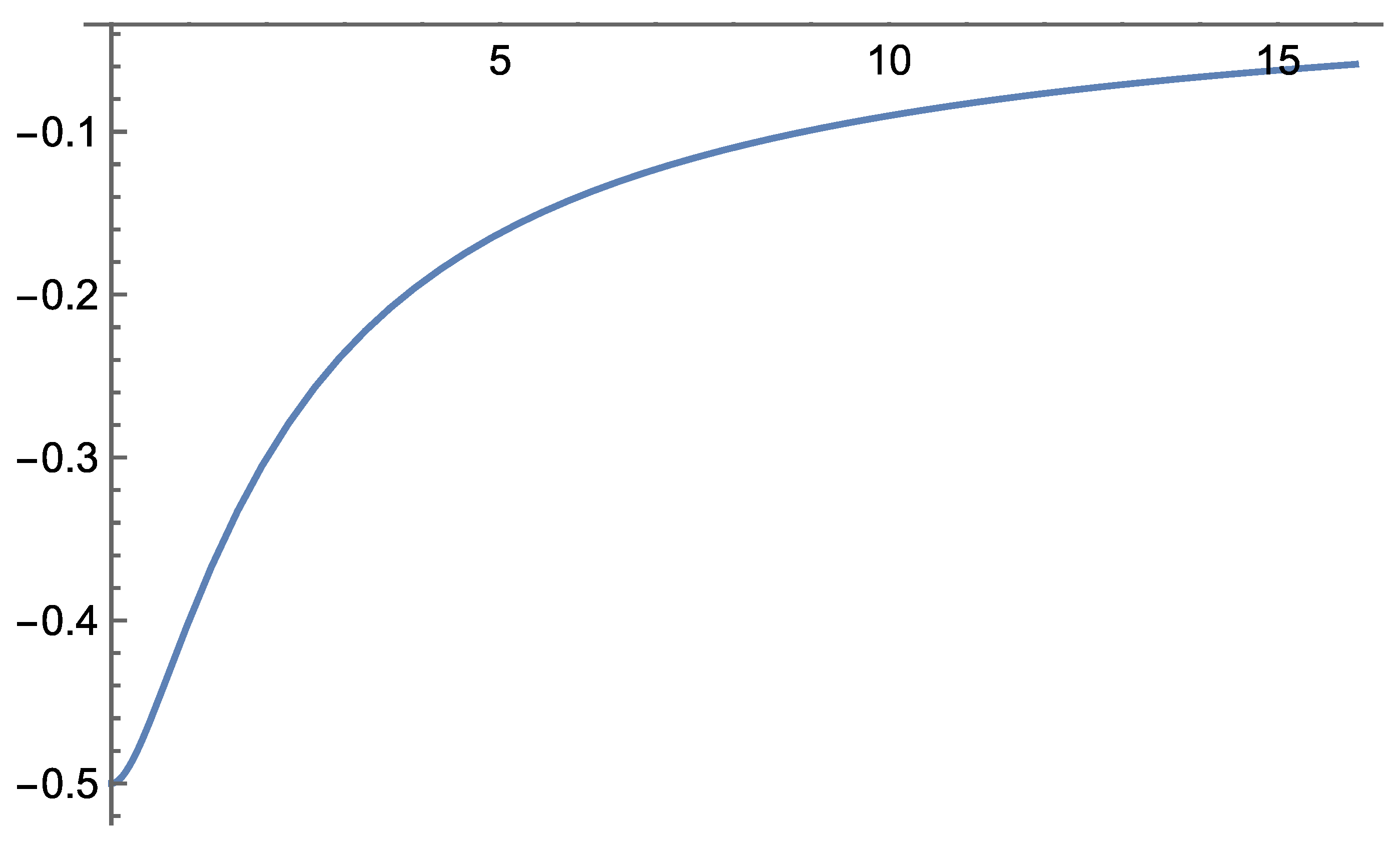
Figure 4.6.
Interaction I. The function if . Source: Figure by author.
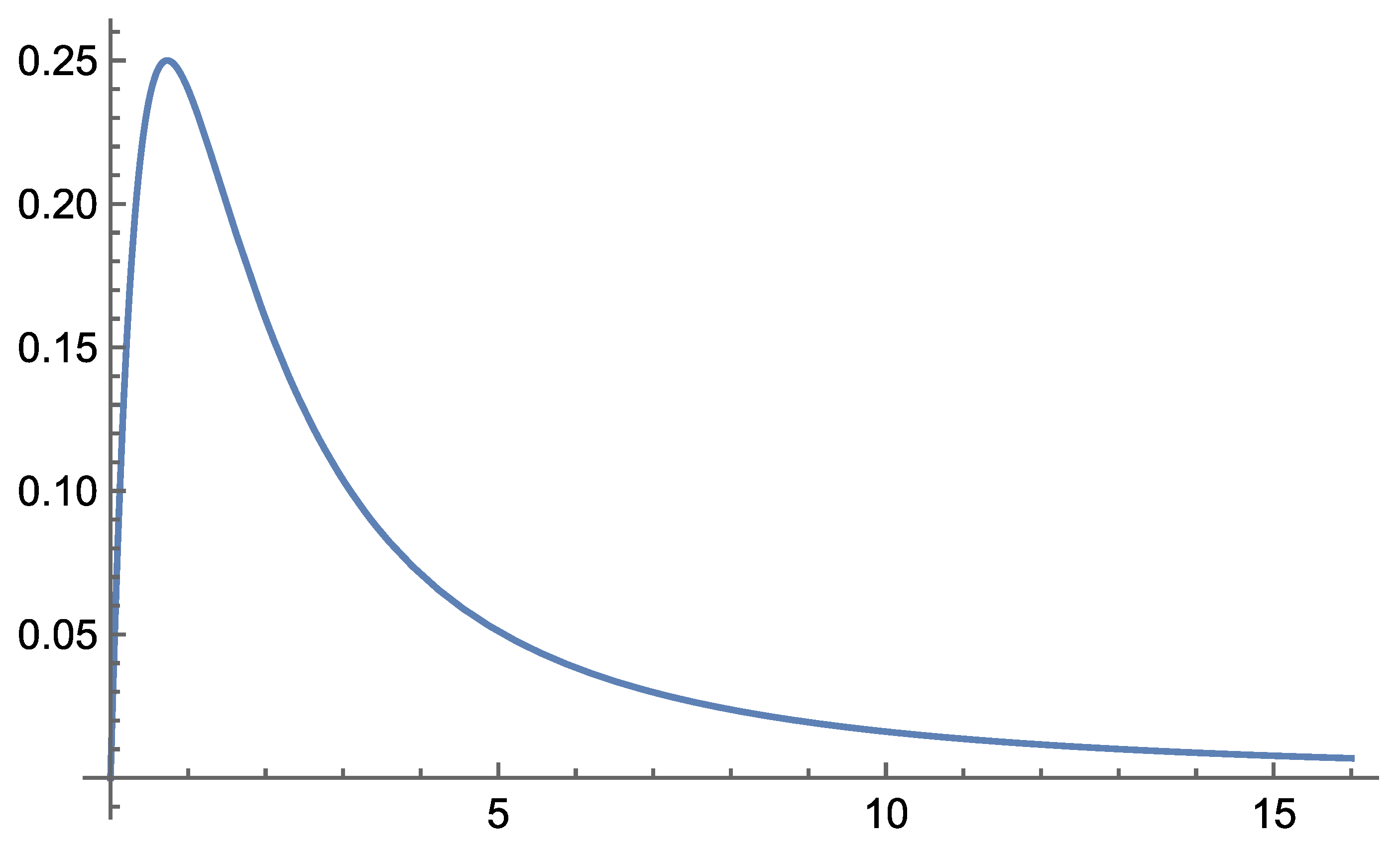
Figure 4.7.
Interaction I. The function if . Source: Figure by author.
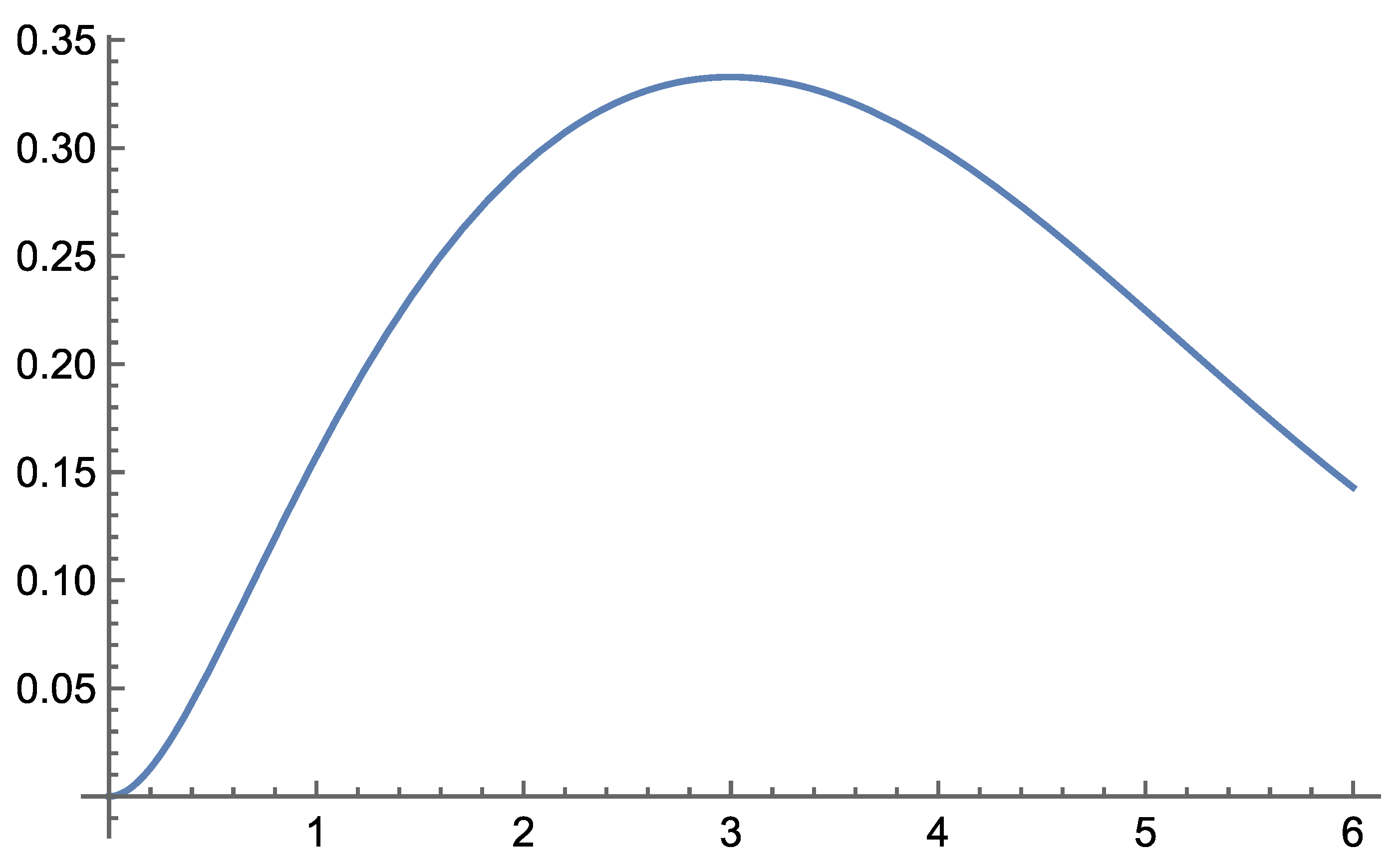
Figure 4.8.
Interaction I. The function if . Source: Figure by author.
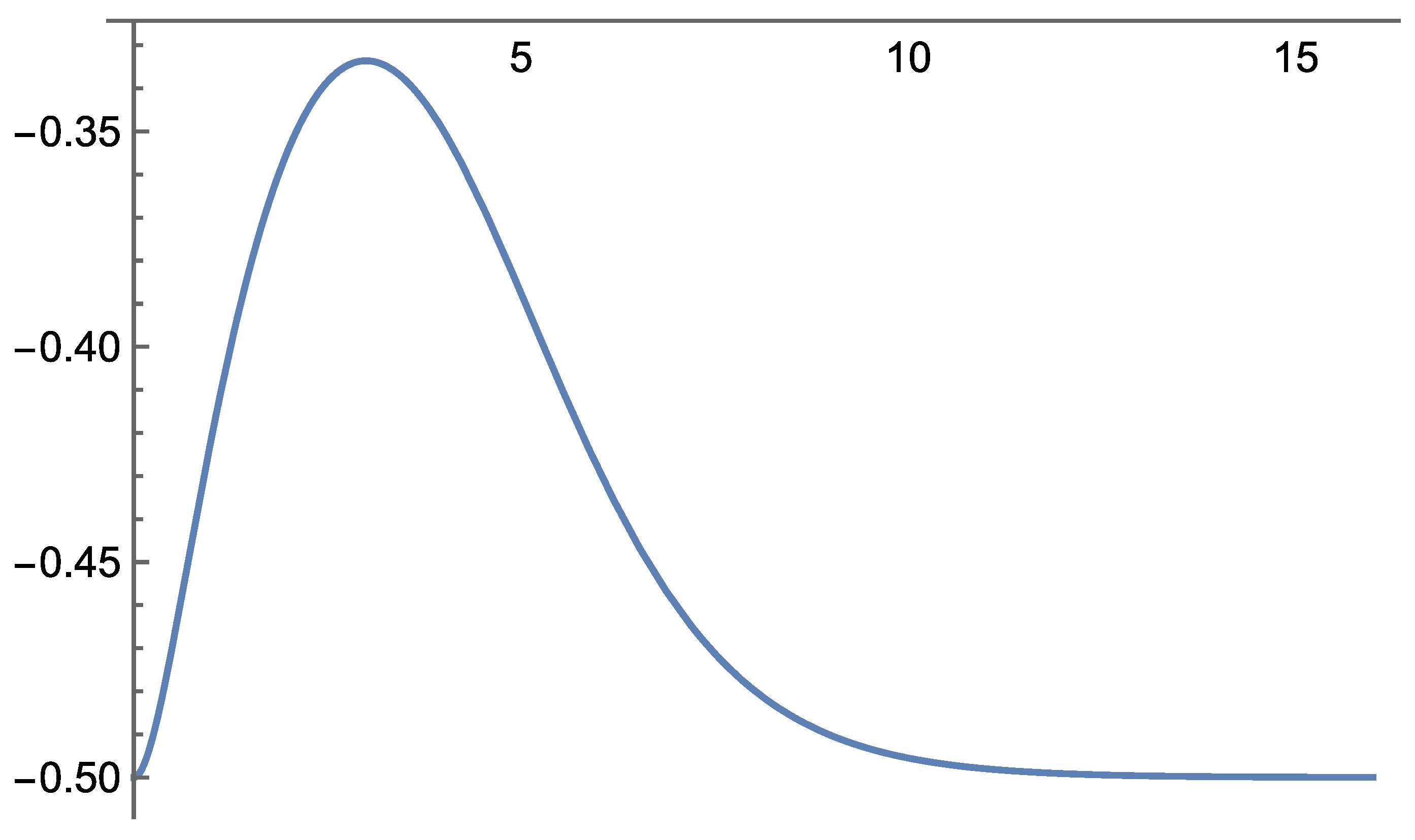
Figure 4.9.
Interaction I. The function if . Source: Figure by author.
Interaction II
Figure 4.10.
Interaction II. The function if . Source: Figure by author.
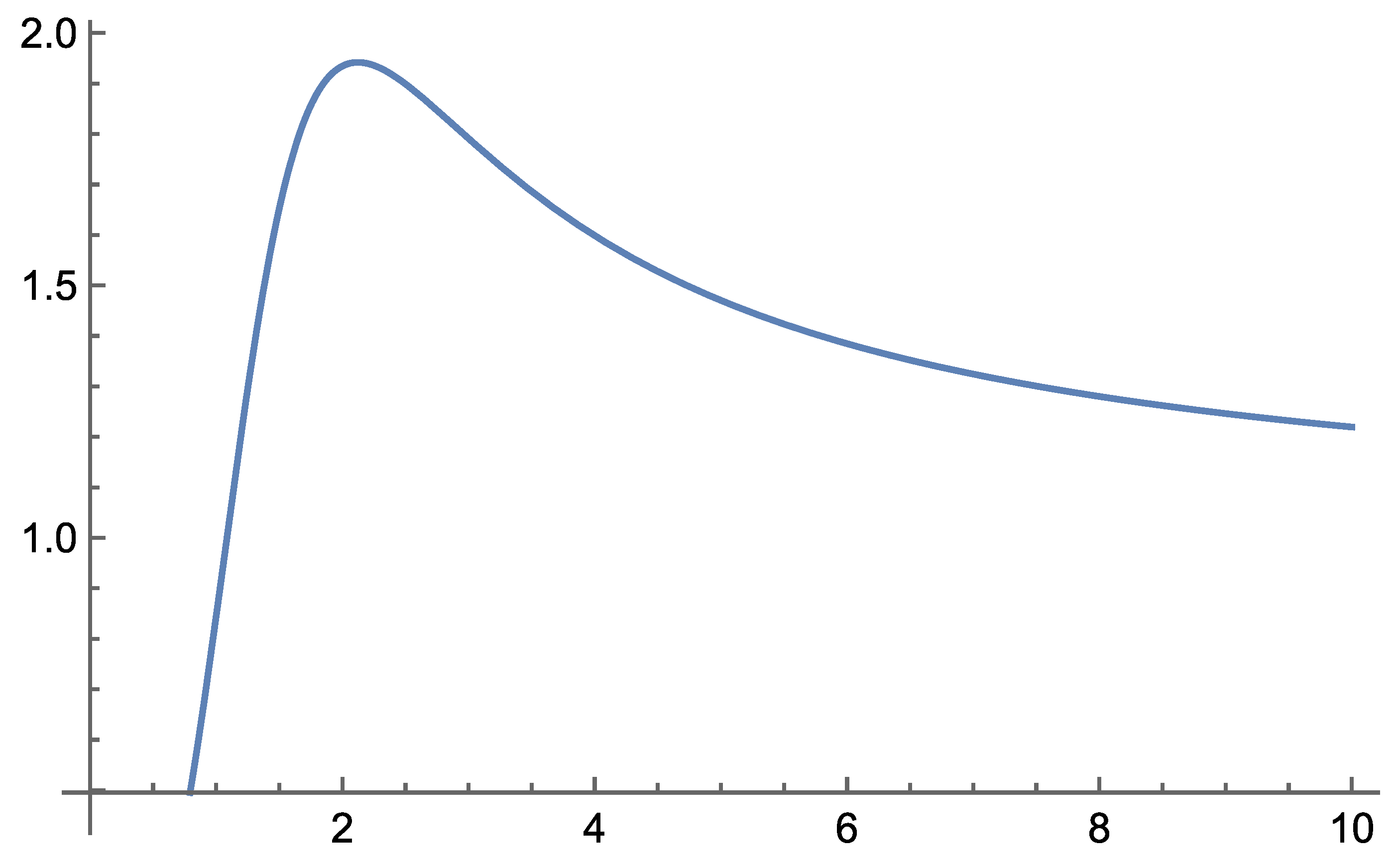
Figure 4.11.
Interaction II. The function if . Source: Figure by author.

Figure 4.12.
Interaction II. The function if . Source: Figure by author.
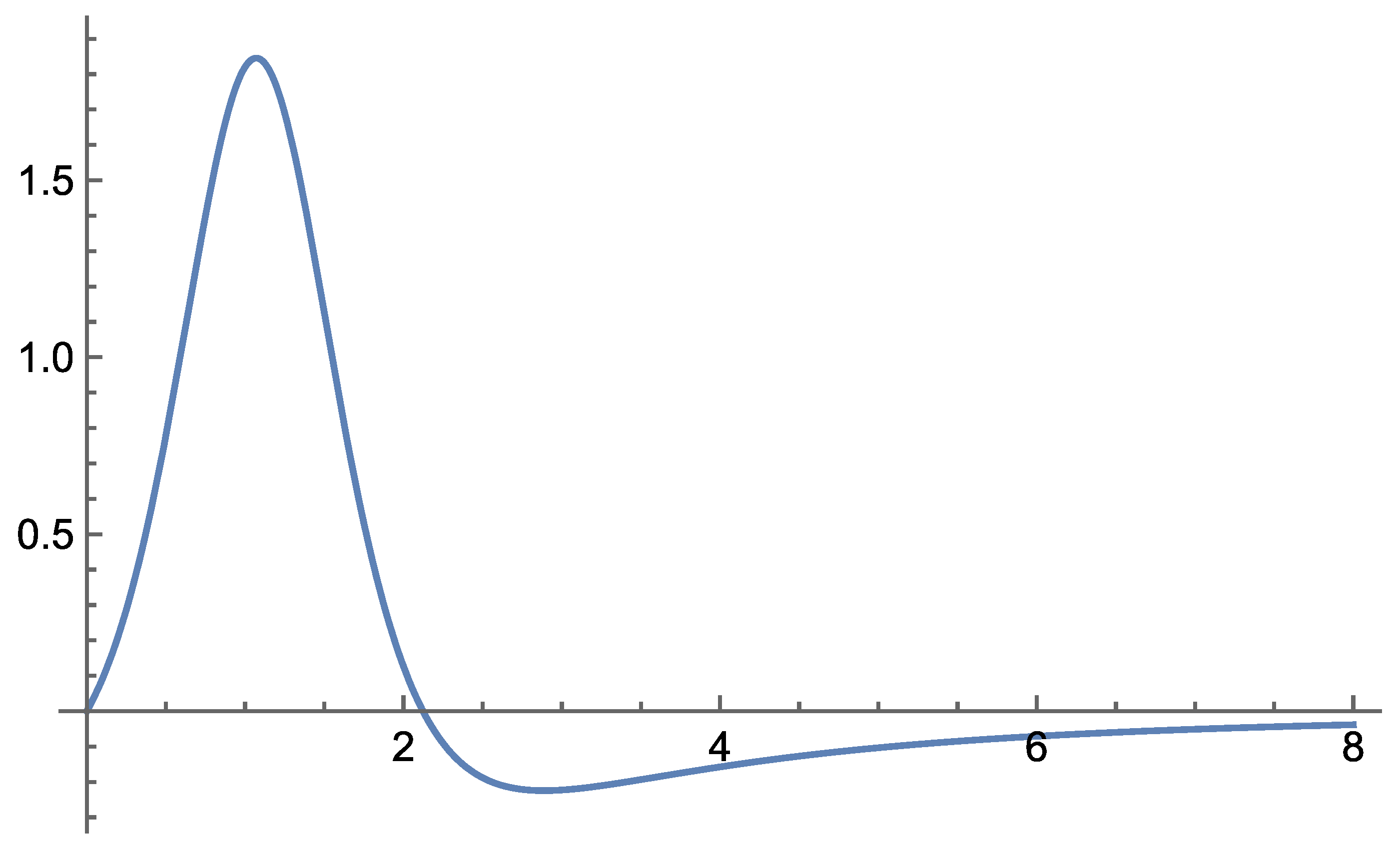
Figure 4.13.
Interaction II. The function if . Source: Figure by author.
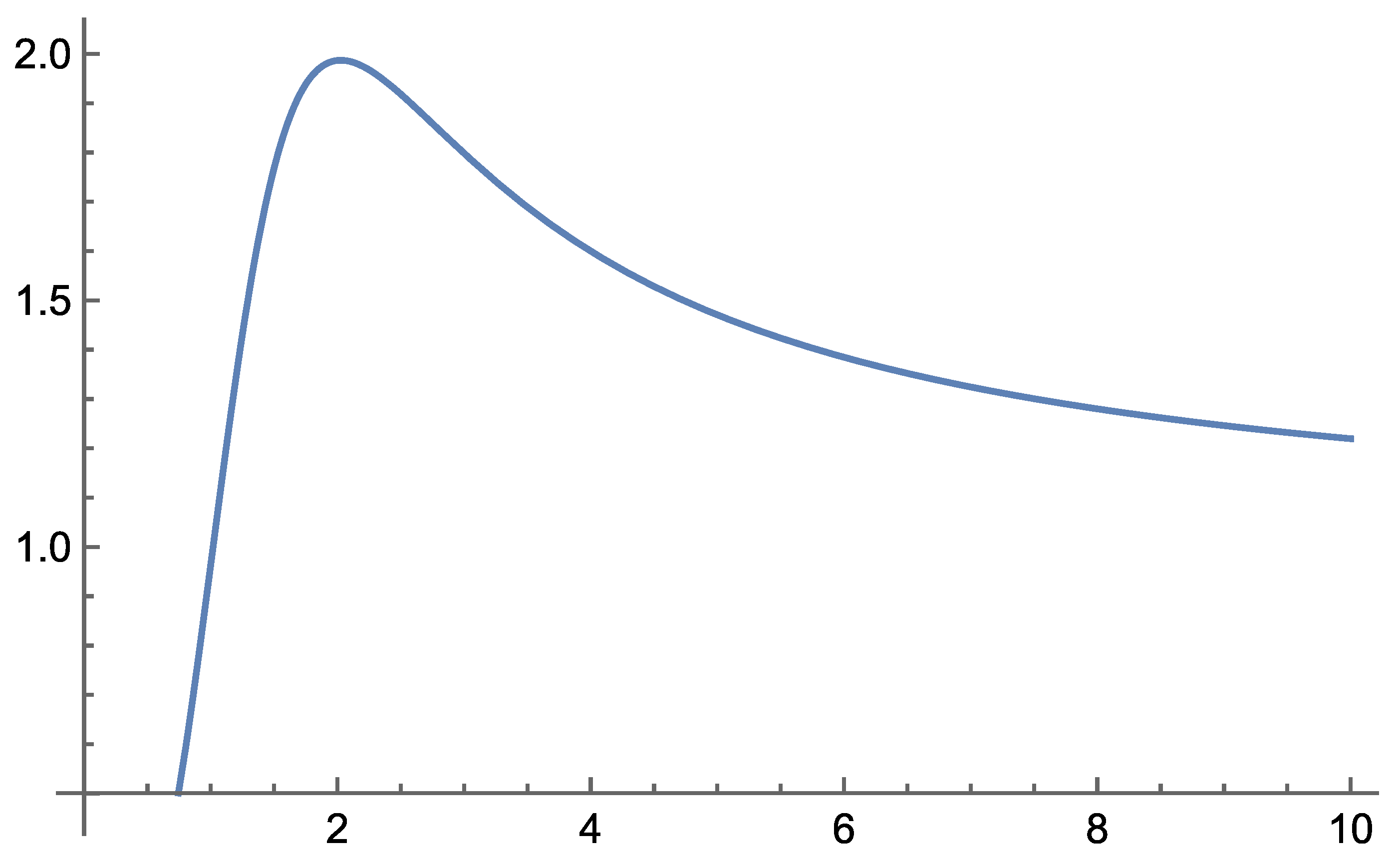
Figure 4.14.
Interaction II. The function if . Source: Figure by author.
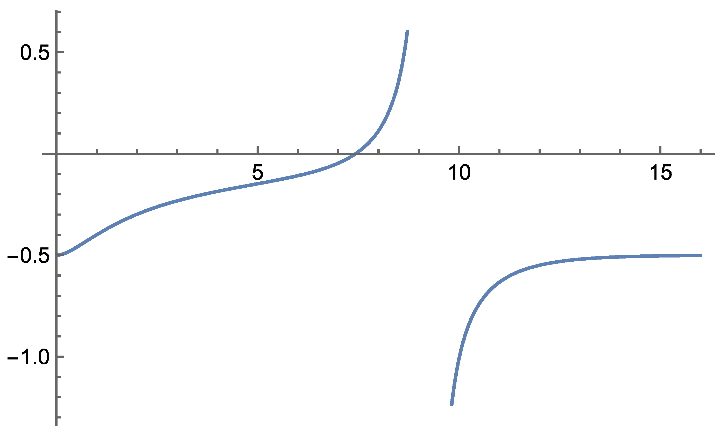
Figure 4.15.
Interaction II. The function if . Source: Figure by author.

Interaction III
Figure 4.16.
Interaction III. The function if . Source: Figure by author.
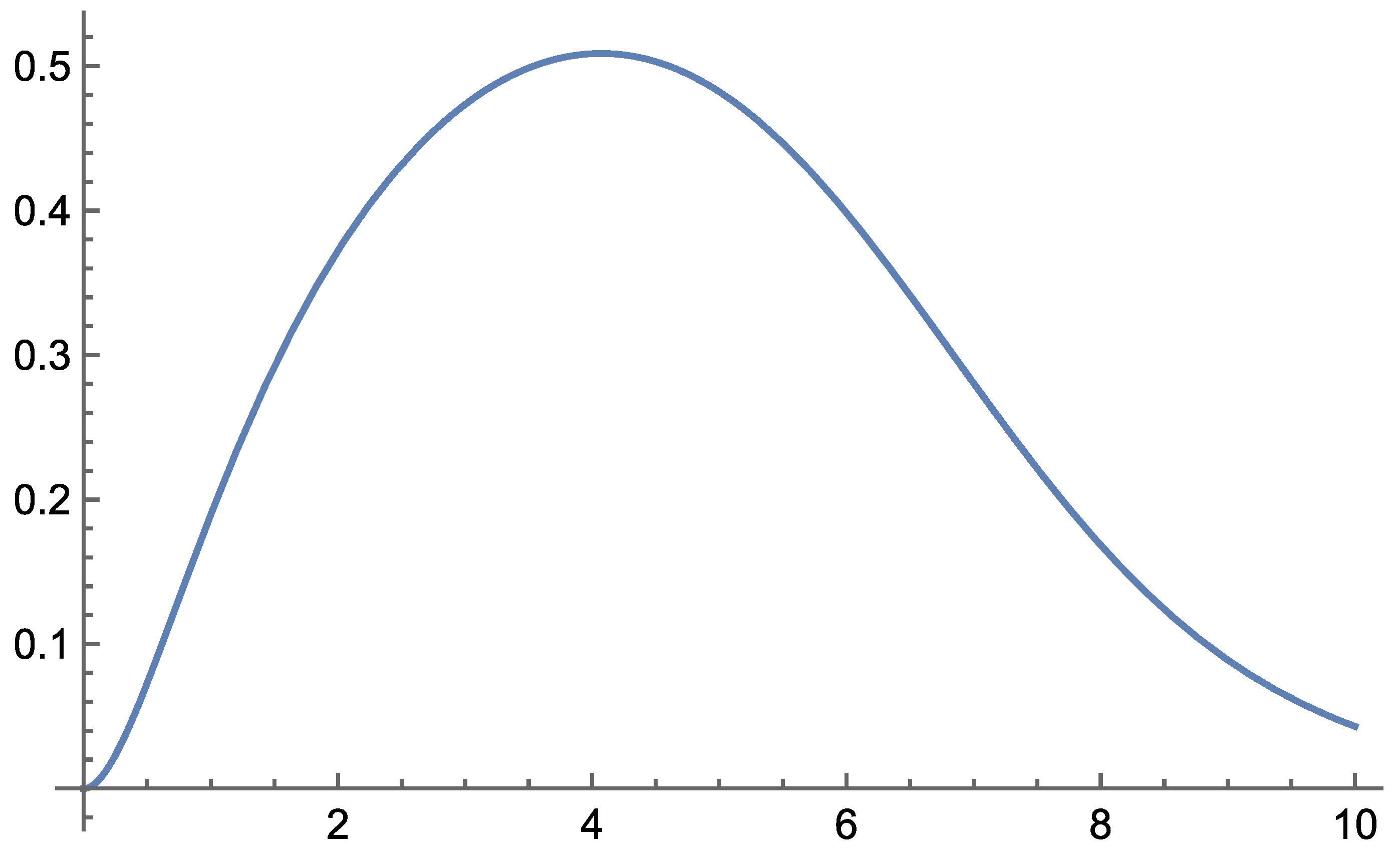
Figure 4.17.
Interaction III. The function if . Source: Figure by author.
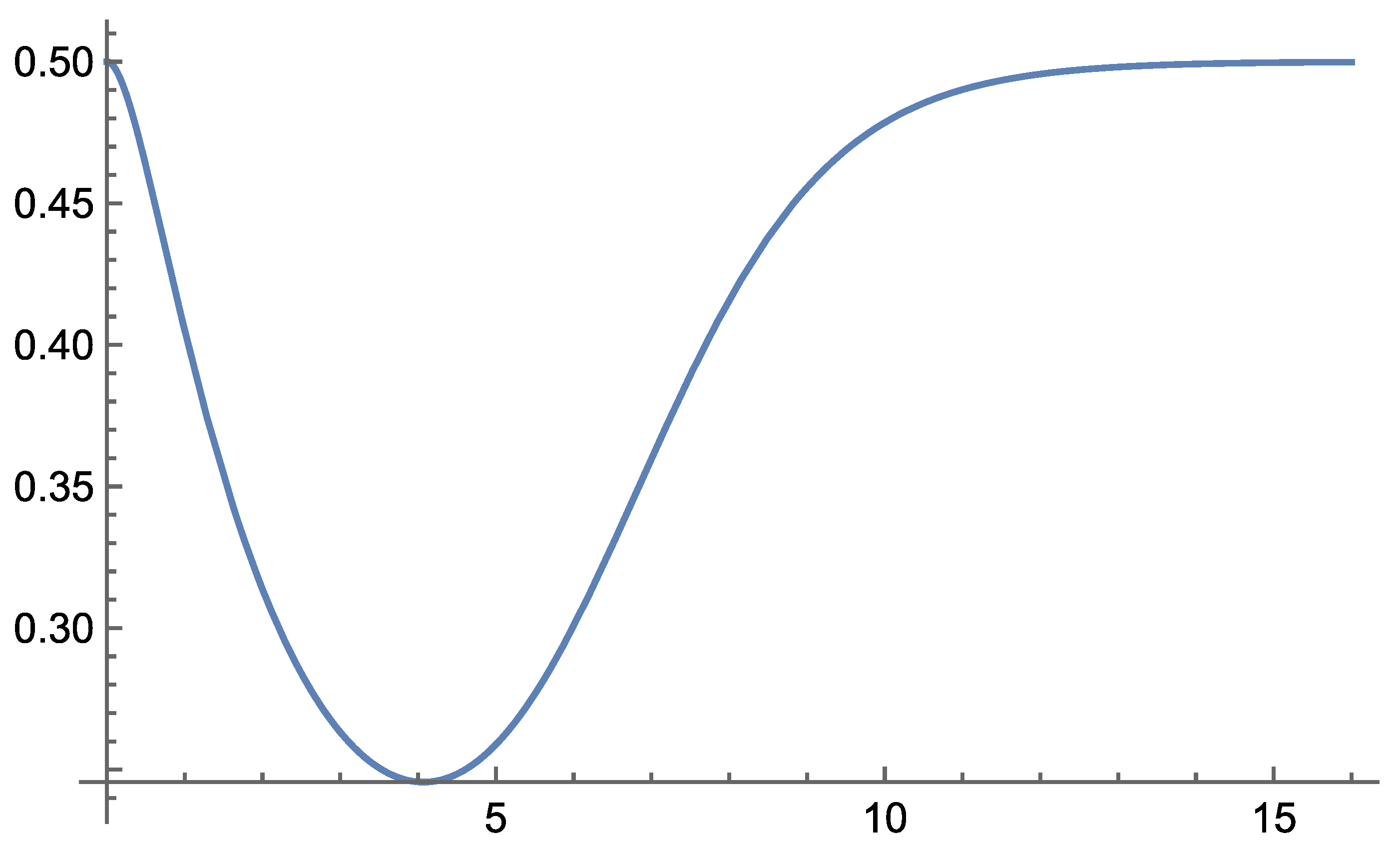
Figure 4.18.
Interaction III. The function if . Source: Figure by author.
Interaction IV
Figure 4.19.
Interaction IV. The graph of the function if , \, , and . Source: Figure by author.
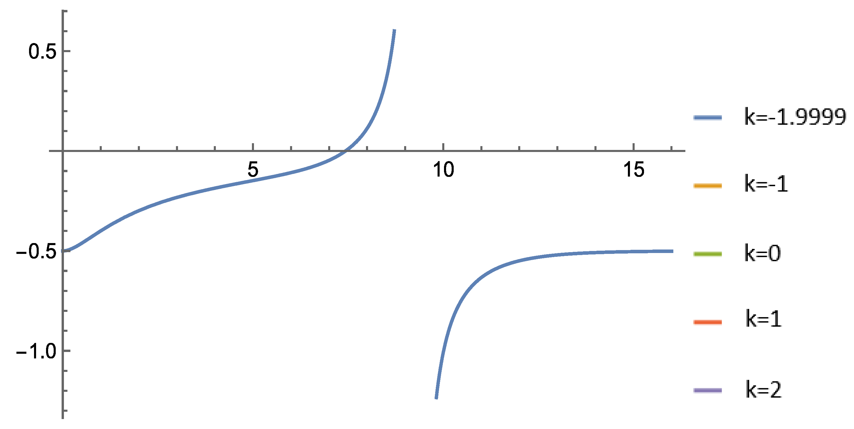
Figure 4.20.
Interaction IV. The graph of the function if , , and . Source: Figure by author.
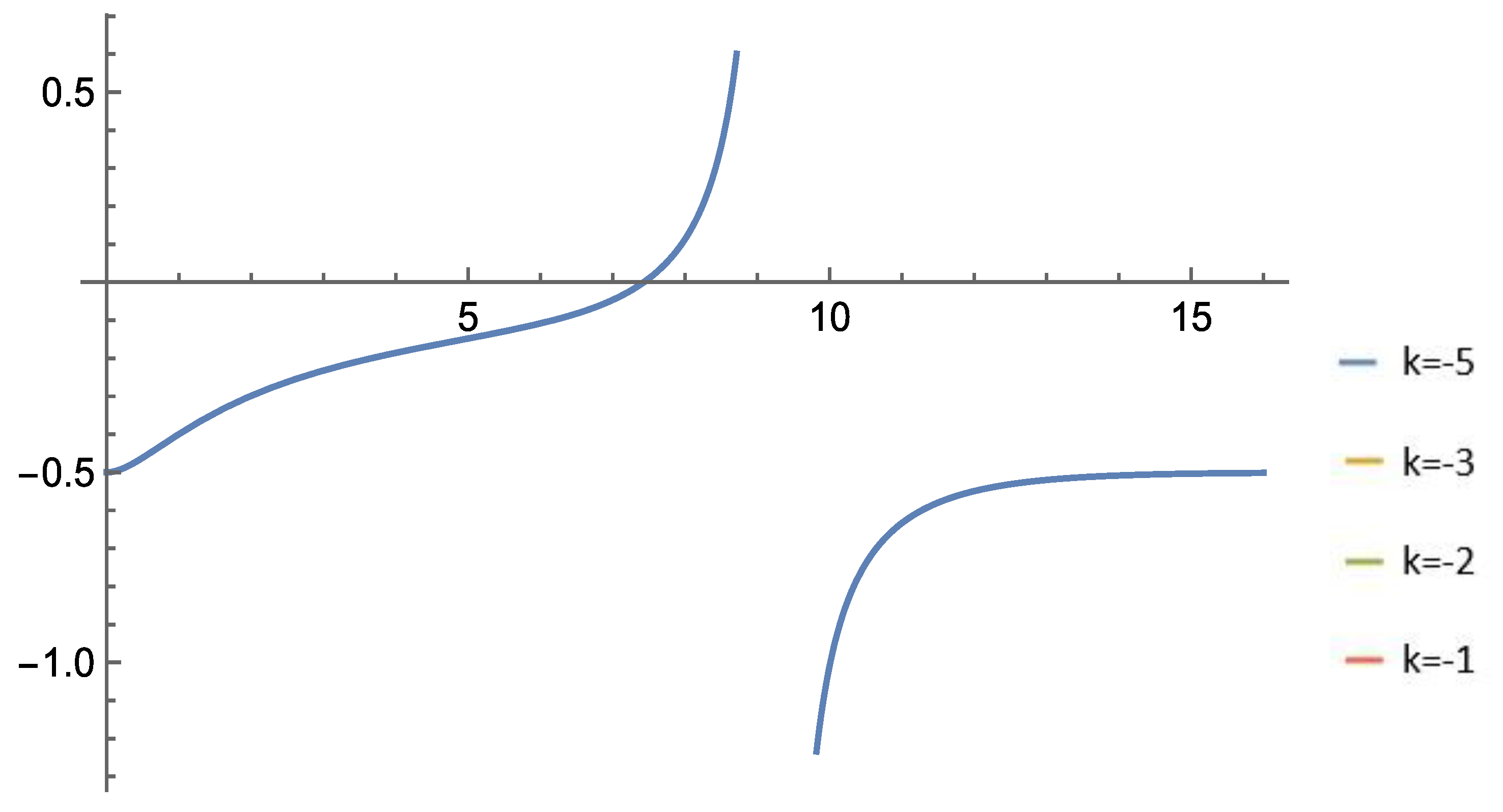
Figure 4.21.
Interaction IV. The graph of the function if . Source: Figure by author.
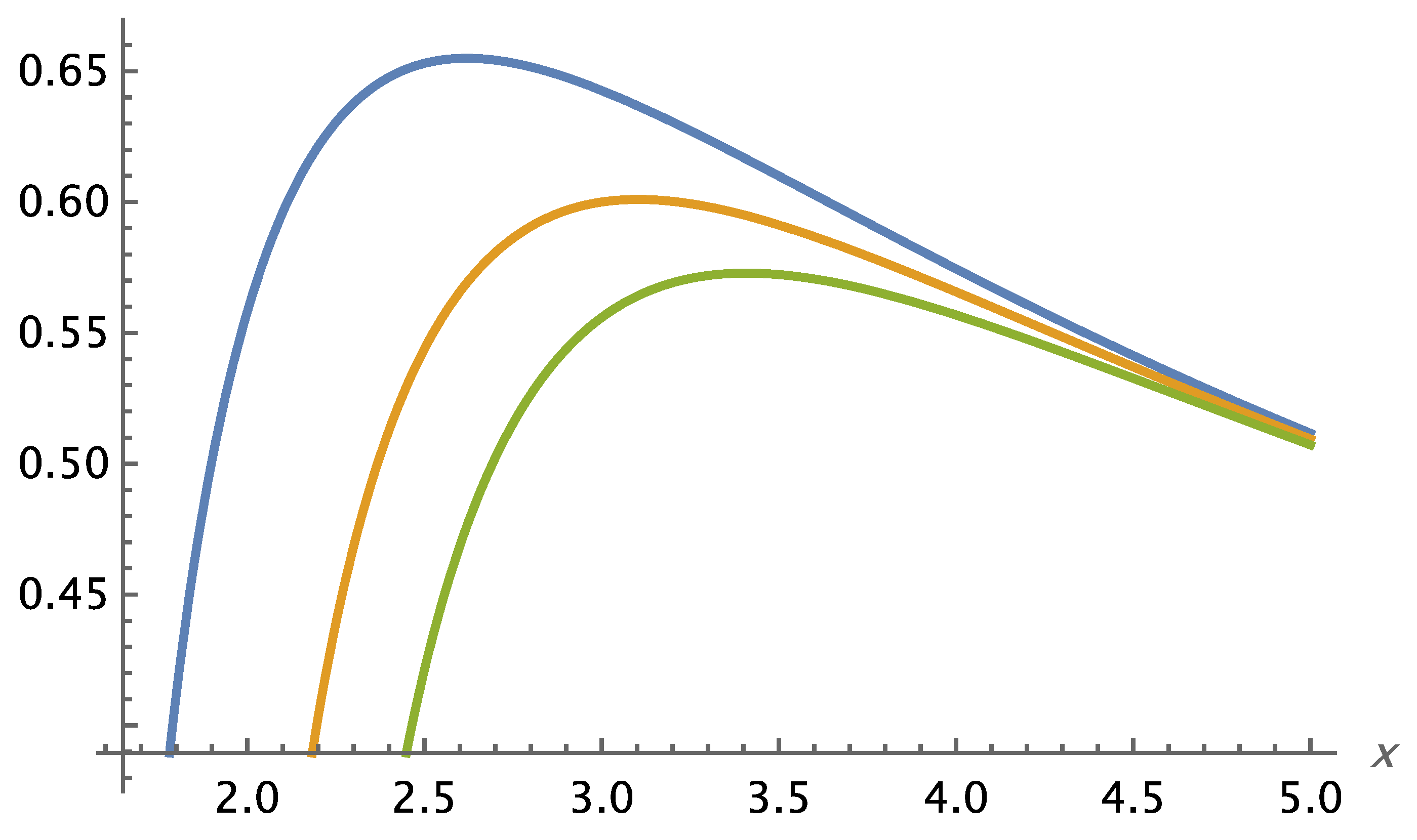
Figure 4.22.
Interaction IV. The graph of the function if . Source: Figure by author.
4.4. Rotational Velocities Around the Mass M in Interaction IV
The rotational velocities around the point mass are described by Equation
In the case of Interaction IV, the corresponding potential is given by Equation (4.19). Substituting into this Equation, we obtain the rotational velocity profile around the mass for this specific interaction:
, where (4.29)
Below, we present diagrams of the function for various values of the parameter . Subsequently, a comparative plot is provided, illustrating the rotational velocities in Interaction IV alongside the corresponding Newtonian values,
Figure 4.23.
Interaction IV. The graph of the function if , for small values of . Source: Figure by author.
Figure 4.23.
Interaction IV. The graph of the function if , for small values of . Source: Figure by author.
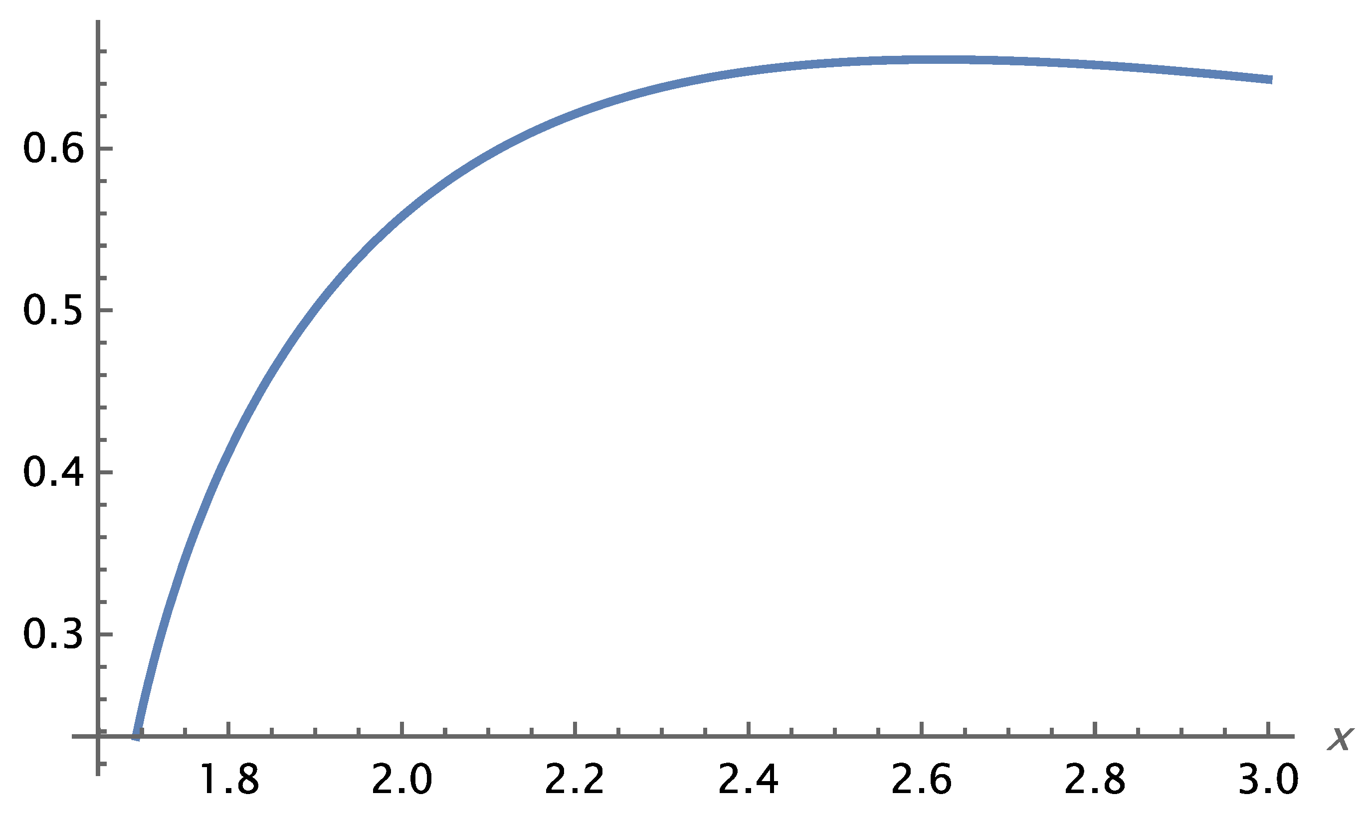
Figure 4.24.
Interaction IV. The graph of the function , if , for large values of . Source: Figure by author.
Figure 4.24.
Interaction IV. The graph of the function , if , for large values of . Source: Figure by author.
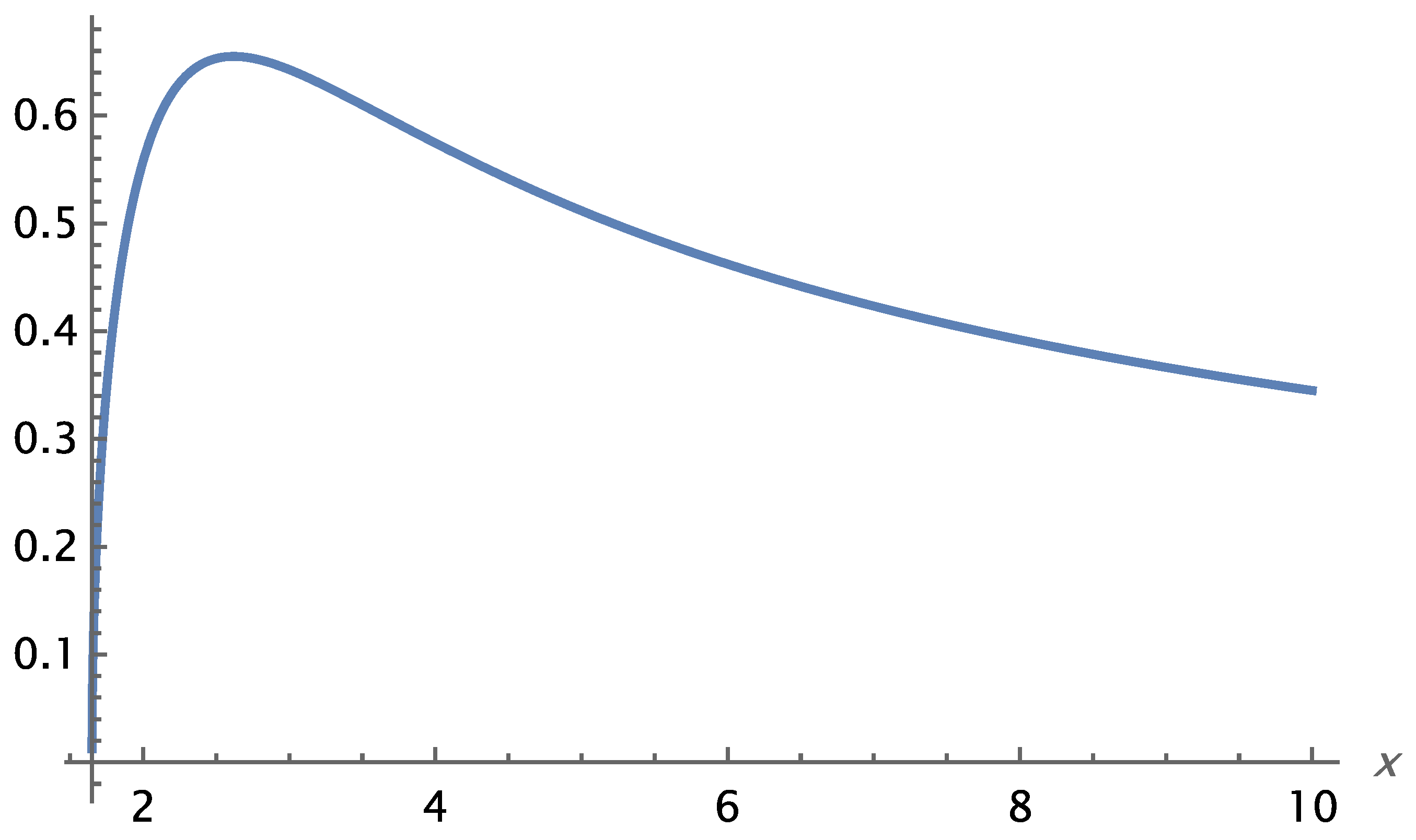
Figure 4.25.
Interaction IV. The graph of the function if , and . Source: Figure by author.
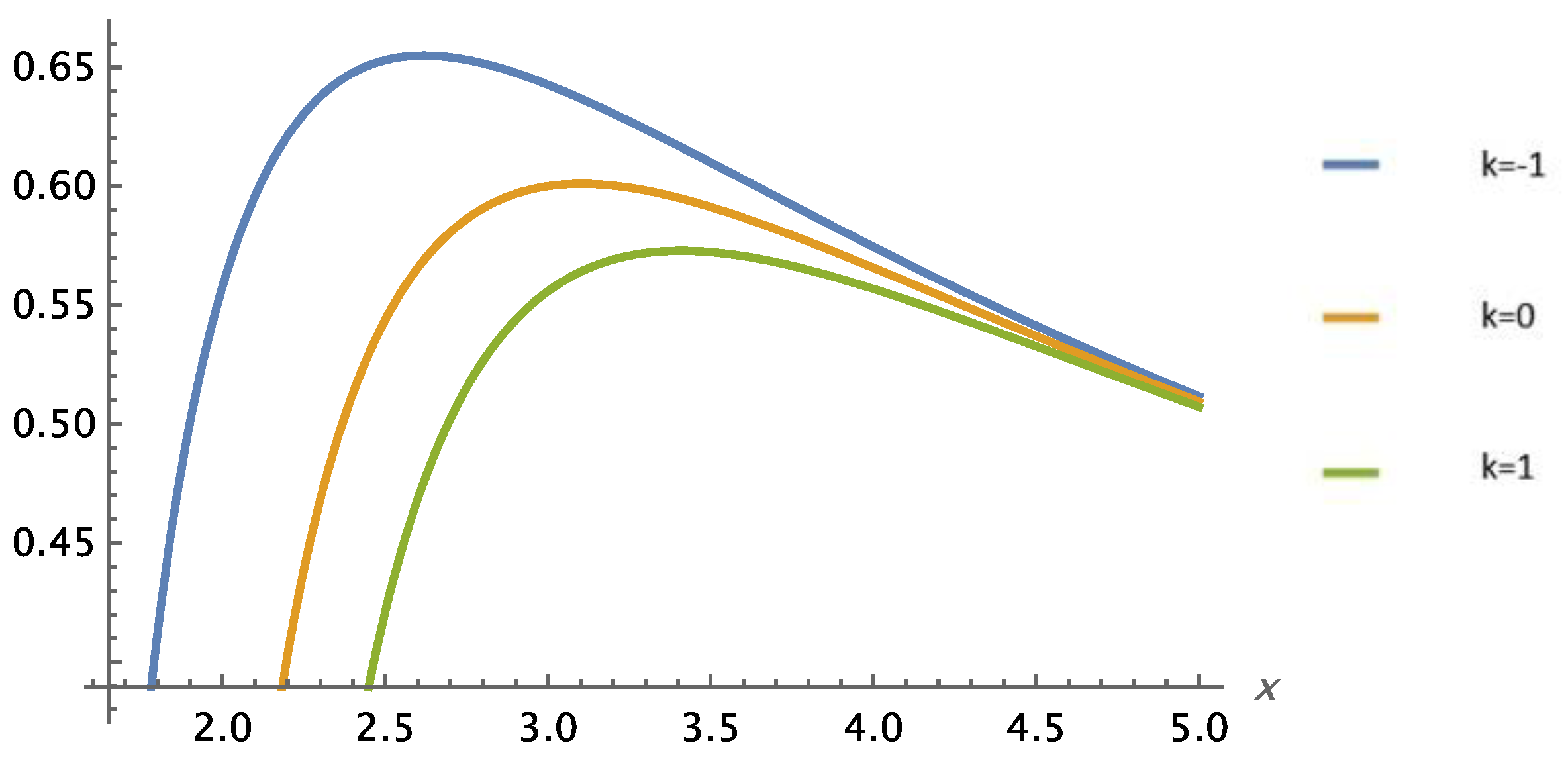
The deviation between observational data and the predictions of Newtonian gravity and General Relativity [2,3,5,17] has been documented in several studies [36,37,38,39,40,41], [84,85,86]. This discrepancy was first identified by Fritz Zwicky [44], who proposed the existence of Dark Matter—a form of matter that contributes to the gravitational field but does not interact with electromagnetic radiation, and is therefore not directly observable. Subsequent observations reinforced the mismatch between theory and data, thereby solidifying the Dark Matter hypothesis as a necessary extension to the standard theoretical framework.
Diagrams 4.24, 4.25, and 4.26 correspond to data already present in the observational literature [36,37,38,39,40,41], [84,85,86]. The predicted rotational velocities shown in these diagrams depend on the parameter , as determined from Equation (4.29).
These diagrams refer to the gravitational field of a point-like rest mass . In order to obtain more accurate predictions for extended astrophysical systems—such as galaxies or galaxy clusters—the spatial distribution of matter must be taken into account. Improved velocity profiles can be derived by applying suitable mathematical models at the appropriate distance scales.
In any case, starting from the field equations for a point mass, one can generalize the formalism to obtain the gravitational field for continuous mass distributions.
We now present a comparative diagram showing the rotational velocity profiles predicted by Interaction IV alongside the corresponding Newtonian prediction. The curve associated with Interaction IV depends on the value of the parameter . In this diagram, three representative values of have been selected to illustrate the variation in the rotational speed.
Figure 4.26.
Interaction V. Comparison of the Newtonian prediction for the rotational velocities with the prediction of the Self-Variation Theory if , and . Source: Figure by author.
Figure 4.26.
Interaction V. Comparison of the Newtonian prediction for the rotational velocities with the prediction of the Self-Variation Theory if , and . Source: Figure by author.
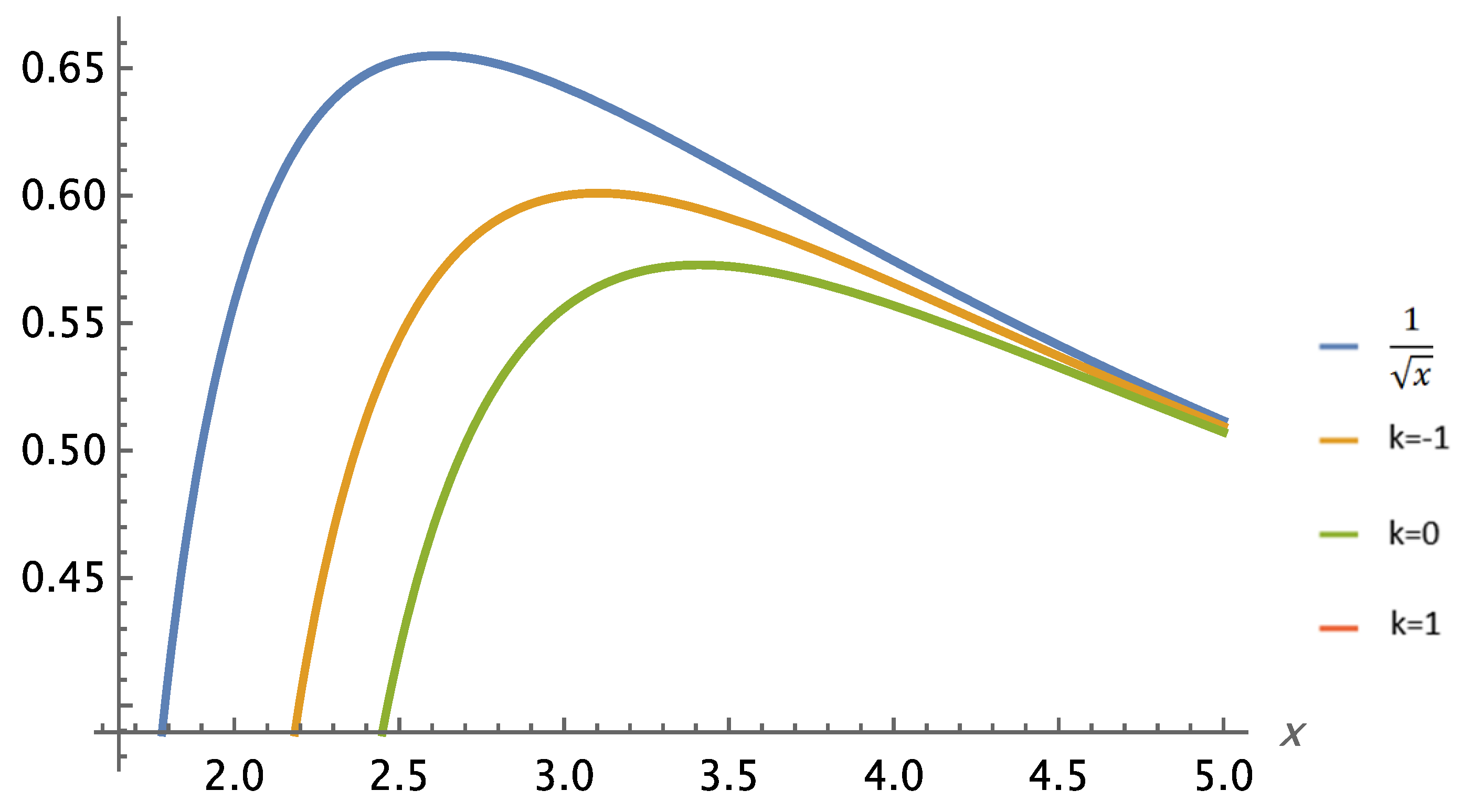
4.5. Interaction I as a Model for Gravity
The propagation velocity, potential, and field strength associated with Interaction I are given by Equations (4.9), (4.10), and (4.11), respectively.
We first observe that the nature of the interaction depends critically on the sign of the parameter . When , the interaction is attractive at short distances but becomes repulsive beyond a certain critical radius (see Figure 4.3). For , the interaction remains purely attractive at all distances (Figure 4.5). When , the interaction is again attractive at all distances, but its functional behavior differs from the case (Figure 4.9), exhibiting a distinct radial dependence.
In what follows, we show that for , Interaction I effectively models gravity, both in qualitative behavior and functional form. Setting in Equations (4.9), (4.10), and (4.11), we obtain the following expressions:
The interaction does not collapse at (i.e., ). This is a common feature of the first group of interactions, I–IV.
For large values of , the potential asymptotically approaches the form
Applying Transformation (4.6), this yields
which corresponds to the Newtonian gravitational potential.
Thus, at large distances from the point mass, the interaction potential converges to the Newtonian form. This asymptotic behavior is also observed in several of the other interactions, although not universally. The general behavior of mass interactions across scales is still not fully understood.
Applying Transformation (4.6) to the potential yields an expression of the form
Through the sequence of simplifications
we obtain,
. (4.30)
Equation (4.30) can alternatively be derived by expanding the potential V(x) as a Taylor series around infinity, expressed in terms of 1/x,
Applying Transformation (4.6) to this expression leads directly to the form
as given in Equation (4.30). The extra term provides a negligible correction to the overall potential.
The first term in Equation (4.30) recovers the classical Newtonian potential. The second term introduces a correction, quantifying the deviation from Newtonian gravity. We proceed to analyze the implications of this correction. First, we calculate the precession of the perihelion of the planets per orbit.
We solve the differential equation of the orbit in polar coordinates , for the potential given in Equation (4.30). We start with the general form of the differential equation for a central force,
where
and is the specific angular momentum per unit mass (a constant, due to conservation of angular momentum). From Equation (4.30), we obtain,
Substituting into the orbital differential equation, and performing the necessary calculations, we find,
The remainder of the proof follows standard procedures and leads to the final result,
for the precession of the perihelion of the planets per orbit, where is the semi-major axis of the orbit and is the eccentricity. The form is similar to that of General Relativity [87,88], where there we have
So the Self-Variation Theory replaces , where c is the speed of light in a vacuum, with the parametric constant . SVT reproduces the Mercury experiment [89,90] (43” of arc per century) if .
We analyze how the presence of the mass affects the curvature of a light ray passing at a minimum distance .To calculate the deflection of light by a mass, we can use the refractive index and apply the equation for deflection,
. (4.31)
To calculate the deflection of light by a mass, we can use the refractive index and apply the equation for deflection,
, (4.32)
where is the minimum distance (radius of closest approach). From Equations (4.31) and (4.30) we obtain the effective refractive index predicted by the SVT for light ,
. (4.33)
From Equations (4.32) and (4.33) we get
. (4.34)
An estimate of the parameter was derived from the observed precession of the planetary perihelia. By substituting this value into Equation (4.34), we obtain a prediction for the angular shift,
Notably, this result is in excellent agreement with the corresponding prediction of General Relativity in the large distance limit [17,91,92],
The contribution of the second term in Equation (4.34) is negligible relative to that of the first term. The angle of bending of light that we get from relation (4.34), in the case of the Sun, is the well-known Δϕ≈1.75 arcseconds [93,94,95].
We now calculate the Shapiro delay resulting from Potential (4.30). The time delay of light caused by the gravitational field is approximated by:
where , are the distances of the transmitter and receiver from the mass mass . The delay in General Relativity [96] is given by:
In Section 4.3, Figures 4.4, 4.5 and 4.6 present the
Calculations based on the point-mass equations have the advantage of being independent of the spatial distribution of matter. In contrast, the equations of the Self-Variation Theory are highly sensitive to this distribution, primarily due to the nature of the Transformation (4.6),
. (4.35)
Consequently, the results obtained for the perihelion precession of the planets and the deflection of light near the Sun are representative of the predictive framework of the theory.
Starting from the equation
. (4.36)
The resulting expression explicitly reveals the dependence of the rotational velocity on the ratio , highlighting the fundamental role of the mass distribution in shaping the rotational dynamics.
We now provide a brief summary of the implications of the potential , intentionally foregoing detailed mathematical treatments that cannot be fully addressed within the constraints of this publication.
Implications at Stellar Scales
At the scale of stars, the finiteness of the potential at () implies the avoidance of classical gravitational singularities during gravitational collapse. This suggests that the SVT potential may provide a natural mechanism preventing infinite density states, thereby stabilizing stellar cores and potentially altering late-stage stellar evolution scenarios. The smoothness of near the stellar radius further supports stable equilibrium configurations without invoking exotic states of matter.
Implications at Galactic Scales
At galactic scales, the SVT potential modifies the gravitational field in a manner that could explain observed anomalies in stellar rotation curves without the need for additional dark matter components. The asymptotic behavior of , decaying more gradually than a pure Newtonian potential, induces a modified gravitational acceleration profile capable of sustaining flat or slowly declining rotation velocities in spiral galaxies. Furthermore, the finite potential near the center aligns with observations of galactic cores lacking definitive singularities, hinting at alternative structures for supermassive compact objects.
Implications at Galaxy Cluster Scales
Extending to the scale of galaxy clusters, the SVT potential supports stable large-scale gravitational binding without requiring substantial amounts of unseen mass. The mild decay of the potential at large distances facilitates gravitational cohesion across cluster scales, potentially reconciling observed mass distributions with luminous matter alone or with less reliance on dark matter hypotheses. This could also affect gravitational lensing profiles and cluster dynamics in a measurable way.
Building on the previous discussion, we now examine the consequences of the fact that the field propagation speed varies with distance from the source. In the general case, the field propagation velocity is given by the relation
The requirement imposes two simultaneous constraints: the parameter must take small negative values, , and the variable must remain within a limited range of small values. When considering a concentration of matter within a spatial region whose size is determined by the constraint on , two important conclusions emerge:
The propagation velocity of the gravitational field within this region remains strictly subluminal, .
The velocity can, in principle, attain its upper limit at the boundary or in the outer vicinity of the region. This second observation is of particular relevance when the gravitational field propagates beyond the localized matter distribution. In such a case, where the field spreads into the surrounding space with constant velocity , the causal structure and physical consequences of gravity may differ from those discussed in the previous paragraph.
In the general case of the potential (4.10) of interaction I, the rotational velocities are given by the system of equations:
. (4.37)
This functional relationship captures the dependence of the predicted interaction term I on the parameters , and the quotient , in the context of rotational velocities of stars within galaxies and of galaxies within galaxy clusters.
A simplified form of the interaction was used in our application. However, the general Equation (4.1) encapsulates a significantly richer structure, containing substantially more information about the interactions involving mass.
4.6. The Role of the Parameters and in SVT Gravity
From the potential Equations the role of the parameters and emerges.
The role of the parameter in SVT gravity.
1. Physical interpretation of the parameter .
The unit of is exactly the unit of gravitational potential. Thus, σ is a characteristic value of the gravitational potential in the context of SVT theory-an energy potential scale.
The parameter determines the ratio between distance and mass:
For a given mass , the length scale (i.e. the distance where the SVT theory starts to deviate from Newtonian) is:
That is:
The larger the mass, the larger the distance where significant divergence appears.
The larger , the closer to the source the non-Newtonian effects appear.
Conversely:
If we observe divergences at distance , then the theory says that they depend on the quantity
That is, the distance of critical deviant behavior increases linearly with mass.
In summary: The divergences appear on different scales for different masses.
2. Geometric interpretation: Space scale variability.
The existence of allows the potential:
To vary in a non-universal way.
To depend not only on the distance , but also on how this distance is “measured” in relation to the mass.
3. Strong connection to cosmological or galactic scales:
If is very small, deviations from Newtonian gravity appear at large distances. Thus, may play a role in explanations such as the pursuit of rotation curves without dark matter.
4. If , becomes a direct measure of how “close” you are to the Schwarzschild radius,
that is, how strong the gravitational field is-as in General Relativity.
So, at this value, the SVT aligns geometrically and dimensionally with GR.
The role of the parameter in SVT gravity.
1. Shape modifier of the potential:
appears within exponential terms, thus modulating the depth or strength of the attenuation with distance via .
If is large, the effect of the exponential term (which indicates rapid attenuation) becomes more significant.
2. Mathematical role:
acts as a modifier of the contribution of the exponential term with respect to the polynomial terms (, ). Thus, it controls the deviation of the SVT potential from Newtonian at small or large distances.
3. Relationship to the limiting behavior of the potential:
For (i.e. ) or for (i.e. ), affects whether the potential approaches zero, a constant, Newtonian, or some other form.
4.7. Symmetries in the Gravitational Field Equations of the Self-Variation Theory
Three distinct symmetries emerge in the gravitational field equations of the Self-Variation Theory. The first symmetry, previously discussed, concerns the division of the eight predicted interactions into two distinct categories, depending on the presence or absence of the exponential integral in their governing equations. Each category comprises four interactions.
The second symmetry involves the substitution in Equation (4.1). Specifically, for interactions I, IV, V, and VIII, the substitution is employed, while for interactions II, III, VI, and VII, the substitution is used. Based on these substitutions, one might expect only the interactions with (i.e., I, IV, V, and VIII) to exhibit gravitational characteristics. However, this is not the case. The gravitational behavior of the interactions is not determined by the sign of .
Instead, a third symmetry arises, which manifests differently in each of the two interaction groups. Under a transformation , any interaction belonging to the first group is mapped to another interaction within the same group. We give the transformation equations for the potential:
In contrast, the equations governing the second group of interactions exhibit a more complex symmetry of the form , where a parameter , in addition to the spatial variable , plays a crucial role. This symmetry reflects a deeper structural distinction in these interactions.
Furthermore, the equations of the second group are marked by the presence of the exponential integral function, which further highlights their mathematical and physical particularities.
4.8. A Concise Comparison of Newtonian Gravity, General Relativity, and the Self-Variation Theory
In Table 4.1 we present a brief comparison of Newtonian gravity, General Relativity, and the Self-Variation Theory, in five themes. Here, the change in direction of the force in the prediction of the Self-Variation Theory arises from the potential (4.19). In none of the five themes do all three Theories agree. Their fundamental differences are a consequence of the different starting points that the three Theories have. Their common point is the Newtonian behavior in the weak gravitational field.

Table 4.1.
A brief comparison of Newtonian gravity, General Relativity, and Self-Variation Theory.
We now present a brief comparison of General Relativity (GR) and Self-Variation Theory (SVT). The comparison is made based on the potential (4.19).
1. The gravitational acceleration in SVT is zero at the center-there is no infinite force as in GR.
2. SVT predicts that gravity does not propagate to the center (it freezes).
3. SVT seems to replace GR black holes with extremely compact objects where the field slows down and the force is zero at the center-without singularity.
Does SVT allow material missions (spaceships, particles, light) to enter and exit the region where GR predicts a black hole?
What GR says (for comparison)
In General Relativity:
An event horizon is defined at:
Nothing can escape, not even light.
Everything is forced towards the center.
Time and space are “reversed” locally.
What does SVT predict?
The potential is finite:
What this means for a spaceship:
The spaceship can approach the center without encountering:
Horizon
Infinite acceleration
“Crushing” by gravitational force.
As it approaches the center, gravity weakens, rather than strengthens.
So no impenetrable zones prevent entry or exit.
However:
Although there is no event horizon, the field “freezes”-the field propagation speed decreases → the dynamic response of spacetime or communication may be greatly delayed.
Unlike GR:
SVT does not prevent anything from escaping the region near the center.
A photon or a body could regain energy and escape.
But-there is a caveat:
If the gravitational field propagation speed is extremely low near the center, then the environment may appear “frozen”: the causality or reaction of the field may be very slow, which may mimic “trapping”, but is not absolute.
5. The Cosmological Data as a Consequence of the Self-Variation of the Material Particles
In this chapter, we explore the cosmological implications of the self-variation principle. According to the theory, the rest mass and electric charge of a particle (more generally, its self-varying charge) appear smaller in cosmological-scale observations than their corresponding values measured in the laboratory on Earth. This has significant consequences for all physical phenomena in distant astronomical objects that depend on these fundamental quantities. These effects are imprinted in observational cosmological data. One prominent manifestation is the redshift of distant astronomical sources.
Many fundamental quantities in astrophysics depend on redshift. As a function of redshift, we compute: the electron mass (and more generally, the masses of fundamental particles), the ionization energy and the degree of ionization of atoms, the Thomson and Klein–Nishina scattering coefficients, the position–momentum uncertainty and the Bohr radius, as well as the energy released in nuclear reactions and hydrogen fusion.
Observational data indicate that the rate of increase of the electron’s charge (in absolute value) is significantly slower than the rate of increase of rest mass. This empirical result is in agreement with the theoretical prediction presented in Section 2.3, where a different growth rate for mass and charge was established as a consequence of self-variation.
One of the more striking implications is that, due to the self-variation of rest mass, gravity does not have cosmological-scale consequences: it is neither responsible for the expansion nor for any potential collapse of the universe. Gravitational effects are instead confined to smaller-scale structures, such as galaxies and clusters.
In Section 5.10, we compare the Standard Cosmological Model (SCM) with the predictions of Self-Variation Theory at cosmological scales. We highlight the reasons why the SCM has been compelled to adopt a series of auxiliary assumptions (e.g. dark energy, inflation, etc.) to align itself with observational data. However, certain observations—such as the two inconsistent measured values of the Hubble constant—currently lack a plausible explanation within the SCM framework.
By contrast, the origin and evolution of the universe as described by the Self-Variation Theory shows remarkable agreement with cosmological observations, offering a coherent and natural explanation for phenomena that remain puzzling under the standard model.
5.1. Rest Mass and Electric Charge on the Cosmological Scale
The reduced values of rest mass in the past time result in the weakening of gravity, compared to its strength on earth and nearby galaxies. This attenuation is extremely large at cosmological-scale distances. The equations given by the Self-Variation Theory predict that gravity cannot cause the universe to collapse or expand. The consequences of gravity are limited to other distance scales, much smaller than the cosmological one.
The Standard Cosmological Model is based on General Relativity. However, it has repeatedly had to introduce additional assumptions in order to bring the Model into agreement with the observational data. From the hypothesis of Dark Matter [36,37,38,39,40,41,42,43,44], [97,98,99,100] and inflation [49,51,72,100,101], to the more recent hypothesis of Dark Energy [66,68]. The Standard Cosmological Model is inconsistent with recent measurements from the early twenty-first century to the present, of the time evolution of the creation of the large-scale structures of the universe [24,45,46,62], [102,103,104]. There is no hypothesis that could bring the Standard Cosmological Model into agreement with the two measured values for the Hubble constant [67,69].
The Internal Symmetry Theorem justifies the so far known cosmological data, in a flat and static universe. We point out that the increased rotational velocities of stars in galaxies and galaxies in galaxy clusters are justified by the conclusions of Chapter 4 regarding gravity (see Section 4.8).
In a flat and static universe, from Equation (2.31) for , we get the following equation for the increase in rest mass to over time ,
. (5.1)
From Equations (2.21) and (2.22), requiring
. (5.2)
In Equation (5.1) the constant is negative.
We consider an astronomical object at distance from Earth. The emission of the electromagnetic spectrum of the far-distant astronomical object we observe “now” on Earth has taken place before a time interval . From Equation (5.1) we have that the rest mass on the distant astronomical object at the moment of emission was,
. (5.3)
From Equations (5.1) and (5.3) we obtain,
. (5.4)
Different particles have different rest mass . Furthermore, in different particles the self-variation can evolve in a different way, which can be expressed by a different value of the constant . Thus in Equation (5.4) we denote,
. (5.5)
With the index ‘ ’ we denote the particle to which the constant refers. With this symbolism, Equation (5.4) is written in the form,
. (5.6)
We now denote by the time-dependent function,
. (5.7)
From Equations (5.6) and (5.7) we obtain,
. (5.8)
From Equation (5.7) we obtain,
. (5.9)
Similarly, starting from Equation (2.33) we get the following equations,
, (5.10)
, (5.11)
, (5.12)
. (5.13)
5.2. The Redshift of the Distant Astronomical Objects
The fine structure constant is defined as
, (5.14)
where is the electric charge of the electron. From Equation (5.11) if the charge of electron we obtain,
. (5.15)
The energy of the electron in the atom is
. (5.16)
From Equation (5.16) we have for the redshift ,
. (5.17)
From Equations (5.15) and (5.17) we get,
. (5.18)
The increase of rest mass to over time is given by Equation (2.31). Considering that the electric charge of the electron contributes a small percentage to its total rest mass, we conclude that in Equations (2.31) and (2.33) is, . If we assume that in the same particle the constant is the same for rest mass and electric charge, then then we conclude that the charge of the electron increases at a much lower rate, compared to the rate of increase of its rest mass . This conclusion is confirmed by the cosmological data [52,73]. Considering that the electric charge of the electron increases at a much slower rate than its rest mass, from Equation (5.18) we get,
. (5.19)
For small distances , from Equation (5.19) we get,
, (5.20)
where is the Hubble constant for the linear spectrum of atoms. If the measurements we make depend on the ΄΄heavy΄΄ particles, such as the proton and neutron, Equation (5.20) becomes,
. (5.21)
The Self-Variation Theory predicts the measurement of at least two values of the Hubble constant [67,69]. On the cosmological scale, the self-variation of the electron and the heavy particles correspond to different values of Hubble’s constant.
Taking into account that , and , from Equation (5.20) we get,
From Equation (5.10) we get,
. (5.22)
From this inequality and considering the possible values of redshift we conclude that,
. (5.23)
The limit (5.23) implies that we can go far back into the past, giving increasingly large values of redshift . The Self-Variation Theory Equations on the cosmological scale are compatible with extremely large values of redshift.
From Equation (5.20) we get,
. (5.24)
From this Equation and limit (5.23) we conclude that Hubble’s constant increases slightly with time. Considering that , the rate of change of Hubble’s constant is equal to its square, . In the context of Self-Variation Theory the Hubble constant is a variable parameter which increases over time, at an extremely slow rate. The same slight increase with time is also predicted for the redshift, for a specific distant astronomical object, which is at a distance . From Equations (5.19) and (5.9) we get,
. (5.25)
From Equation (5.19) we get,
. (5.26)
This Equation gives the distance of a distant astronomical object as a function of redshift . To measure cosmological-scale distances through the redshift requires the measurement of the constant and the parameter . Today we precisely measure the value of the Hubble constant . We also know the possible values of the parameter , as given by the limit (5.23) . Thus we can calculate the possible values of the constant from Equation (5.20).
5.3. The Rest Mass of the Electron as a Function of Redshift
From Equations (5.8) and (5.19) we obtain,
. (5.27)
The redshift is measured with great precision. Therefore, Equation (5.27) gives the relation between and very precisely.
A large set of physical phenomena and mechanisms depend on the rest mass of the electron. Therefore it is important to know precisely its value in distant astronomical objects. This accuracy, for the rest mass of electron, is given by Equation (5.27). Self-Variation Theory gives a number of parameters of physics and astrophysics as a function of redshift. Thus, on the cosmological scale we can measure the effects of self-variation on a distant astronomical object based on redshift, which we measure precisely, rather than based on the object’s distance, which we do not know.
5.4. The Reduced Energies of Distant Astronomical Objects
From Equation (5.27) we get,
(5.28)
for the energy of the electron. Taking into account the two measured values of the Hubble constant, we conclude that Equation (5.28) is also approximately valid for heavy particles. This Equation predicts that the energy resulting from hydrogen fusion and nuclear reactions is reduced in distant astronomical objects. This reduction in energy production likely affects the apparent brightness of distant astronomical objects.
By considering all parameters of astrophysics that are a function of redshift, we can draw conclusions about the luminosity of distant astronomical objects, the amount of light they emits from their surface. Similarly, we can draw conclusions about how redshift affects the time and space evolution of specific mechanisms, such as the accretion of matter due to gravity or the explosion of a supernova.
5.5. The Thomson and Klein-Nishina Scattering Coefficients as a Function of Redshift of the Distant Astronomical Objects
The laboratory value of the Thomson scattering coefficient is given by equation,
, (5.29)
where the rest mass and the electric charge of the electron. Thus we have,
, (5.30)
where is the Thomson scattering coefficient in a distant astronomical with redshift .
The Thomson coefficient concerns the scattering of photons with low energy . For photons with high energy the photon scattering is determined from the Klein-Nishina coefficient,
(5.31)
in the laboratory and,
(5.32)
in an astronomical object with redshift . From Equations and (5.28) we get,
. (5.33)
From Equation (5.33) we conclude that the Thomson and Klein-Nishina scattering coefficients increase with redshift and in the same way.
From Equation (5.19) we obtain,
. (5.34)
Then from Equations (5.33) and (5.34) we get,
. (5.35)
Considering the limit (5.23) and Equation (5.35) we conclude that the Thomson and Klein-Nishina scattering coefficients had enormous values in the very early universe. In its initial phase the universe was totally opaque. From this initial phase of the evolution of the universe originates the Cosmic Microwave Background Radiation [54,65] we observe today.
5.6. The Ionization and Excitation Energies of Atoms as a Function of Redshift of the Distant Astronomical Objects
The ionization energy as well as the excitation energy of atoms is proportional to the factor , where is the rest mass and the electric charge of the electron. Therefore we have,
. (5.36)
From Equation (5.36) we conclude that the ionization and excitation energies of atoms decrease with increasing redshift. This fact has consequences on the degree of ionization of atoms in the distant astronomical objects.
The number of excited atoms in a gas in a state of thermodynamic equilibrium is given by Boltzmann’s equation [83],
, (5.37)
where is the number of atoms at energy level , the excitation energy from the 1st to the nth energy level, Boltzmann’s constant, the temperature in degrees Kelvin, and the multiplicity of level , i.e. the number of levels into which level is split apart inside a magnetic field.
From Equations (5.36) and (5.37) we obtain,
. (5.38)
From Equation (5.38) it follows that as takes extremely large values, the quotient tends to quotient . This limit is independent of the temperature and the laboratory excitation energy from the 1st to the nth energy level. The real constraint in Equation (5.38) concerns the redshift values for which the hydrogen atom has structured. We will look at this limitation in the next Section 5.7.
For the hydrogen atom for , , , and at the surface of the Sun where , Equation (5.37) implies that just one in atoms is at state , i.e. . From Equation (5.38) we get the corresponding quotient as a function of redshift . If we have , if we have , if we have , and if we have .
If we have .
To estimate the temperature at high redshift values, it is essential to account for the decrease in energy release from hydrogen fusion and other nuclear processes, as described by Equation (5.28). Notably, in the limit of very large , the ratio asymptotically approaches the ratio of the . This is a consequence of Equation (5.38),
For large redshift values it is necessary to take into account other parameters to draw conclusions about the conditions that prevailed in the universe. From Equation (5.36) we get . The universe could be ionized. Moreover, from Equation (5.33) we get . The very large values of the Thomson and Klein-Nishina scattering coefficients suggest an opaque universe. In any case, it follows from equations (5.36) and (5.38) that in the past, the universe went through an ionization phase of possibly long duration.
5.7. The Position-Momentum Uncertainty as a Function of Redshift of the Distant Astronomical Objects
Combining Equations (2.23) and (5.7) we have,
. (5.39)
From the position-momentum uncertainty [80], for the axis we have,
. (5.40)
From Equation (5.40) we conclude that the uncertain of position of a material particle increases with the redshift. Moreover, as the universe evolved towards the state we observe today, the uncertainty of position of material particles was decreasing.
From Equations (5.40) and (5.34) we have,
. (5.41)
Considering the limit (5.23) and Equation (5.41) we conclude that in the very early universe there existed great uncertainty of position of material particles. As a consequence of Equation (5.27), the same conclusions arise for the Bohr radius,
As a function of redshift it is given by the equation,
(5.42)
and its limiting value in the very early universe is given by the equation,
. (5.43)
From equation (5.40) it follows that as the redshift increases, so does the uncertainty of the position of the material particles. From Equation (5.41) it follows that the uncertainty of the position of material particles in the very early universe tends to infinity. In the very early universe, from a redshift value and up, all points in the universe communicated with each other.
From Equation (5.43) it follows that the Bohr radius in the very early universe tends to infinity. From Equation (5.42) it follows that as the redshift increases, the Bohr radius in the hydrogen atom also increases. Therefore, from one value of the redshift and above there is no electromagnetic interaction proton-electron. In the distant past, from a value of redshift and above the hydrogen atom has not yet been structured. In the early universe there is no linear electromagnetic spectrum.
5.8. On the Type Ia Supernovae
The production of energy in the universe is mainly through hydrogen fusion and nuclear reactions. Therefore, the energy produced in the past at distant astronomical objects was smaller than the corresponding energy produced today in our galaxy (refer to Equation (5.28)). Reduced energy production indirectly affects the brightness of distant astronomical objects. Fundamental parameters of astrophysics depend on redshift. The dependence of these parameters on redshift can also affect the brightness of distant astronomical objects. Increased values of the Thomson and Klein-Nishina scattering coefficients (refer to Eqqation (5.33)) reduce the luminosity of an ionized gas cloud. There are cases in which the reduced masses of material particles affect the brightness of distant astronomical objects. Reduced masses mean greater agility of material particles.
A characteristic example concerns type Ia supernovae. The value of the rest mass of the electron, given as a function of the redshift from Equation (5.27), plays a defining role at all phases of evolution of a star which ends up exploding as a type Ia supernova. The same is true for the reduced mass of the hydrogen atom. Another factor affecting the luminosity of type Ia supernovae is the increased value of the Bohr radius in the hydrogen atom, compared to its laboratory value. As a consequence of Equations (5.27) and (5.42) the intrinsic luminosity of supernovae of type Ia supernovae depends on redshift. The dependence of brightness on redshift is recorded at the seemingly long distances of type Ia supernovae [66,68]. Type Ia supernovae cannot be used as standard candles for measuring distances on the cosmological scale.
5.9. The Evolution of the Universe. Vacuum State
From Equation (5.36) it follows that as the universe evolved to the state we observe today the ionization energy increased. This prediction is generally valid for any kind of negative dynamical energies which bind together material particles to produce more complex particles.
From Equation (5.28) we have,
From Equations (5.27) and (5.34) we have,
. (5.44)
Considering the limit (5.23) and Equation (5.44) we conclude that, as the universe tends toward its initial state, the rest masses of material particles tend to zero,
. (5.45)
With the notation we follow, from Equations (2.22) and (5.7) we have,
, (5.46)
According to relations (5.45) and (5.46) the initial state of the universe tends asymptotically to zero. Taking into account all kinds of negative potential energy in the structures of the universe, on microscopic and macroscopic scales, we conclude that the total mass / energy of the universe asymptotically tends to zero or is zero. We called this initial state of the universe the “Vacuum State.” Taking into account the conservation of energy-momentum we conclude that the universe, as a whole, is permanently in the Vacuum State (in the sense that its total energy content tends to zero or is equal to zero), at every moment In time, In all phases of Its evolution.
As a consequence of the Vacuum State, the gravitational interaction cannot play the role attributed to it by the Standard Cosmological Model. Gravity cannot cause either the collapse or the expansion of the universe.
The gravitational interaction strengthens with the passage of time, as the rest masses of material particles increase. From one point and on this is in position to accumulate matter within “small” regions of space. The role of gravity is limited to the creation of the large structures of the universe.
Based on the Equations of the Self-Variation Theory at the cosmological scale, for each value of the redshift we get a corresponding value of the astrophysical parameters. Therefore, these Equations make it possible to theoretically predict the evolution of the universe from its initial state to its most recent form, as we observe it in our galaxy.
5.10. A Comparison of the Cosmological Predictions of Self-Variation Theory Versus the Standard Cosmological Model, Based on the Cosmological Data
In this Section we compare the predictions of the Standard Cosmological Model and the Self-Variation Cosmological Model, based the fourteen main cosmological data. The interpretation of physical reality, the physical world, is based on the available Theories of Physics. This also applies to the cosmological data. We could say that the Standard Cosmological Model is based on twentieth century Theories of physics. However, this is not accurate. Theories of the twentieth century, by themselves, do not justify the cosmological facts. Their justification requires a series of additional assumptions which do not follow from the Theory but have been introduced into the Standard Cosmological Model in order to bring it into agreement with the cosmological data. The Dark Matter hypothesis was made to make twentieth-century theories of gravity compatible with observational data on large structures of matter, galaxies and galaxy clusters. Despite decades of effort, and the large quantity required to play the role attributed to it, so far no Dark Matter particles have been observed. The inflation hypothesis is not self-consistent and the length of time it is assumed to have lasted is arbitrary. The Dark Energy hypothesis was made under the weight of observational data. Measurements of cosmological-scale distances via Type Ia supernovae were made to confirm the slowing rate of expansion of the universe, as predicted by twentieth-century theories of gravity. The measurements gave the opposite results. Dark Energy was a still needed addition to the theoretical background of the Standard Cosmological Model. The observed flatness of the universe and the two measured values of Hubble’s constant are completely incompatible with the Standard Cosmological Model.
The Self-Variation Theory reasons cosmological data as a consequence of the self-variation of fundamental particles. The cosmological facts result from the combination of the three principles of the Theory and no additional hypothesis is required. Equations (5.27), (5.36), (5.38), (5.33), (5.40), (5.42) and (5.28) give seven astrophysical parameters as a function of redshift . These parameters are the mass of the electron and in general the mass of the fundamental particles, the ionization energy and the degree of ionization of the atoms, the Thomson and Klein-Nishina scattering coefficients, the position-momentum uncertainty and the Bohr radius , and the energy produced in nuclear reactions and hydrogen fusion,
These equations predict the observed cosmological data, with the sole exception of the variation of the fine-structure constant, which is specifically addressed by Equation (5.11). The implications of the redshift-dependence of the astrophysical parameters are found to be in complete agreement with all currently available cosmological observations. This agreement is by no means self-evident. In principle, a parameter—or a combination of parameters—varying with redshift could lead to discrepancies with the data. In such a case, the validity of the Self-Variation Theory would be called into question.
It is important to emphasize that the Self-Variation Theory, being axiomatically constructed, does not permit the introduction of ad hoc assumptions external to its foundational framework in order to reconcile its predictions with observations. Apart from the three core principles on which it is based, the theory introduces no further hypotheses to achieve consistency with cosmological data. All resulting conclusions arise strictly from the mathematical consequences of these foundational principles.
In what follows, we present a detailed comparison between the predictions of the two models, with respect to each of the fourteen principal cosmological observables.
5.10.1. Origin of the Universe
The justification for the redshift also determines the predictions of a Cosmological Model for the origin and evolution of the universe. The different justification of the redshift by the Standard Cosmological Model (expansion of the universe, macroscopic cause) and by the Self-Variation Theory (self-variation of material particles, microscopic cause) lead to completely different predictions about the origin and evolution of the universe.
Going back in time, in the distant past the Standard Cosmological Model predicts the Big Bang as the beginning of the universe. The same prediction is made by the related Cosmological Models which justify the red shift through the expansion of the universe. The Self-Variation Theory predicts as the beginning of the universe a completely different state, the Vacuum State. In the distant past, the early universe differed little or not at all from the vacuum.
In summary, the justification given by each Model for the origin of the universe is as follows.
Standard Cosmological Model; Big Bang.
Self-Variation Cosmological Model; Vacuum State.
5.10.2. Redshift
The phenomenon of cosmological redshift has played a pivotal role in shaping our understanding of the universe. Beginning in 1912, Vesto Slipher was the first to observe that most spiral galaxies exhibit redshifted spectra—an observation that would later underpin fundamental cosmological theories [70]. Edwin Hubble, studying redshift with Milton Humason, established a correlation between a galaxy’s redshift and its distance from Earth—a relationship that laid the groundwork for what would eventually become the Standard Cosmological Model [50].
However, Hubble himself remained cautious in interpreting the physical significance of redshift. In a 1931 letter to Willem de Sitter, Hubble wrote:
“Mr. Humason and I are both deeply sensible of your gracious appreciation of the papers on velocities and distances of nebulae. We use the term ‘apparent’ velocities to emphasize the empirical features of the correlation. The interpretation, we feel, should be left to you and the very few others who are competent to discuss the matter with authority.”[53]
This cautious tone was not a passing sentiment. As Allan Sandage later emphasized, Hubble maintained a degree of skepticism about the expanding-universe interpretation until the end of his life:
“…To the very end of his writings, he maintained this position, favouring (or at the very least keeping open) the model where no true expansion exists, and therefore that the redshift represents a hitherto unrecognized principle of nature.”[105]
This “unrecognized principle” alluded to by Hubble may find a theoretical framework in the Self-Variation Theory (SVT). According to SVT, the redshift observed in distant astronomical objects could stem from a microscopic cause—namely, the gradual self-variation of the electron’s rest mass over cosmological time.
Traditional interpretations, embedded in the framework of General Relativity and Big Bang cosmology, attribute redshift to the expansion of spacetime itself [1,55,71]. Yet, the electromagnetic spectrum of atoms—particularly the hydrogen atom—is determined by fundamental constants: the electron’s rest mass and electric charge, the electric permittivity of free space, the speed of light in a vacuum, and Planck’s constant. A systematic variation in one or more of these constants, particularly the rest mass of the electron, could also produce the observed spectral shifts, even in a non-expanding (static) universe.
Despite the knowledge of these dependencies [75,82], the possibility that redshift arises from a time-evolving electron mass—or any microscopic variation in physical constants—was not seriously pursued during the 20th century. The dominant narrative has focused almost exclusively on macroscopic explanations, sidelining potentially viable microscopic mechanisms.
SVT challenges this orthodoxy by proposing that redshift may not be evidence of spatial expansion, but rather a signature of temporal evolution in fundamental particle properties. In this light, the redshift becomes a record of physical change over time, imprinted in the spectra of distant objects.
If the predictions of SVT hold, they may provide the theoretical foundation for the “unrecognized principle” that Hubble suspected. This reinterpretation not only revisits the original ambiguity in Hubble’s stance but also opens a new line of inquiry into the nature of cosmic evolution—one that does not necessitate the expansion of the universe, but instead posits a dynamic microphysical substrate.
Summary of Redshift Interpretation in Competing Cosmological Models:
The interpretation of cosmological redshift differs fundamentally between the Standard Cosmological Model and the Self-Variation Cosmological Model:
Standard Cosmological Model:
Redshift is interpreted as a direct consequence of the expansion of the universe. As space itself stretches over time, the wavelengths of photons traveling through it are elongated, resulting in the observed redshift of light from distant galaxies.
Self-Variation Cosmological Model (SVCM):
Redshift is attributed to the self-variation of the electron’s rest mass over cosmological time. In this framework, the electron had a significantly lower rest mass in the distant past (corresponding to higher redshift values), which led to lower atomic transition energies. Consequently, the light emitted by atoms in the early universe appears redshifted when observed today, not because of spatial expansion, but due to intrinsic microscopic evolution in fundamental constants.
5.10.3. Cosmic Microwave Background Radiation
The Cosmic Microwave Background Radiation (CMBR) refers to a faint, nearly isotropic background radiation that fills all of space and reaches Earth uniformly from every direction. It has been firmly established that this radiation does not originate from stars, galaxies, or other discrete astronomical objects. Its spectral energy distribution peaks in the microwave region of the electromagnetic spectrum, and its accidental discovery by Penzias and Wilson in 1964 [54,65] played a pivotal role in confirming and popularizing the Standard Cosmological Model (SCM).
In the context of the SCM, the CMBR is interpreted as a remnant of the Big Bang—the “afterglow” of the primordial fireball. The early universe is thought to have existed as a hot, dense plasma primarily composed of ionized hydrogen. Due to high energy and ionization, Thomson scattering dominated photon interactions, making the universe opaque to radiation. As the universe expanded and cooled, it reached a critical temperature (~3000 K) where protons and electrons could recombine to form neutral hydrogen atoms. This phase, known as the recombination period, occurred roughly 379,000 years after the Big Bang. After recombination, photons could propagate freely without scattering—this is referred to as photon decoupling. These freely streaming photons are now observed as the CMBR, redshifted to an effective blackbody temperature of ~2.73 K.
Moreover, the polarization of the CMBR—an observed and well-measured feature—arises naturally in the SCM due to Thomson scattering in an ionized medium prior to recombination. The consistency of this prediction with observations has contributed significantly to the model’s credibility.
However, the Self-Variation Cosmological Model (SVCM) offers a fundamentally different interpretation rooted in evolving microphysical parameters. According to the SVCM, many fundamental physical constants, including the rest mass and electric charge of the electron, vary over cosmological time. These time-varying parameters influence scattering processes and the opacity of the universe in its early phases.
In this framework, the Thomson and Klein-Nishina scattering coefficients attain extremely large values in the very early universe (as shown in Equations 5.33, 5.35, and the limit in 5.23). These coefficients are heavily dependent on the electron’s rest mass, which is predicted by the theory to approach zero as we move back in time toward the initial Vacuum State. Consequently, the free electron density and the strength of interaction between photons and free electrons would have been sufficient to render the universe highly opaque in its initial phase. This leads naturally to blackbody radiation conditions—essentially predicting the CMBR as an emergent property of the high-opacity, ionized state of the early universe.
Furthermore, the initial ionization of the universe—as deduced from Equations 5.36 and 5.38—also implies that the CMBR should exhibit polarization, aligning with empirical observations. The SVCM, therefore, does not require a singular explosive event (i.e., a Big Bang) to account for the CMBR. Instead, it derives it as a natural consequence of the dynamics of self-varying physical parameters within an evolving universe.
The SVCM formalism allows astrophysical parameters to be expressed as functions of redshift, a quantity that is empirically measurable with high precision. This enables the accurate reconstruction of the universe’s thermodynamic and electromagnetic conditions across its history. Given the precision of the SVCM’s predictive framework, its explanation of the CMBR is presented not as a speculative alternative but as a theoretically grounded and calculable consequence of the model.
Summary: Justification of the Cosmic Microwave Background Radiation in Competing Models
Standard Cosmological Model:
The CMBR is interpreted as a relic radiation from the Big Bang, produced during the recombination period and observed today after redshift cooling to ~2.73 K. Its polarization is attributed to Thomson scattering in the early ionized universe.
Self-Variation Cosmological Model:
The CMBR arises from the extremely high values of the Thomson and Klein-Nishina scattering coefficients in the very early universe, caused by the near-zero electron rest mass in the initial Vacuum State. The resulting high opacity and ionization naturally yield blackbody radiation and its observed polarization, without invoking a primordial explosion.
5.10.4. Increased Luminosity Distances of Type Ia Supernovae
On cosmological scales, the distances of astronomical objects can be estimated via redshift, provided that the exact value of the Hubble constant is known. However, the determination of distances to distant astronomical sources is a considerably more complex issue. The first challenge arises from the very definition of “distance,” as this concept differs in flat versus curved geometries. Observational data indicate that the large-scale structure of the universe is flat; thus, Euclidean geometry can be employed to define the distance of a distant source based on its redshift.
This distance — corresponding to the location of the object at the moment it emitted the electromagnetic radiation currently observed on Earth — is embedded within Hubble’s law. To verify the validity of Hubble’s law, however, one must also be able to determine cosmic distances through independent methods.
Astronomical distances can be measured through a hierarchy of techniques, depending on the scale. At small scales, geometric (trigonometric) methods such as triangulation are employed. For greater distances, astronomers utilize so-called standard candles — celestial objects whose intrinsic luminosity can be inferred from observable properties, such as the periodicity of their brightness. Cepheid variables and other pulsating stars serve as classic examples. In addition, Type Ia supernovae — whose light curves follow a characteristic temporal profile — are used as powerful standard candles. These supernovae exhibit rapid increases in luminosity and emit vast amounts of energy, rendering them visible even in extremely distant galaxies. As such, they are essential tools for constructing the cosmic distance ladder.
One of the most widely used distance measures in cosmology is the luminosity distance, denoted D. It is derived from the observed flux received on Earth, given the known intrinsic luminosity of the source. Since energy spreads spherically, the received flux is inversely proportional to the square of the distance. Importantly, D differs from the geometric (or comoving) distance r, because the total energy emitted may not correspond exactly to theoretical assumptions. If the intrinsic luminosity is lower than expected, D will be overestimated; conversely, if it is higher, D will be underestimated.
The light curves of Type Ia supern”vae ’llow precise determination of their absolute magnitudes, enabling distance estimations across cosmological scales. In the late 1990s, two independent teams — led by Adam Riess [68] and Saul Perlmutter [66] — used Type Ia supernovae to perform long-distance measurements aimed at confirming the deceleration of cosmic expansion. According to the Standard Cosmological Model (SCM), the gravitational influence of matter-energy content should cause a gradual slowing of the expansion rate. Surprisingly, the observational results contradicted these expectations. The measured luminosity distances of Type Ia supernovae were significantly larger than those predicted by the SCM. Two hypotheses emerged to account for this discrepancy:
The characteristic light curve of Type Ia supernovae may differ in distant galaxies compared to those in the Milky Way.
The universe is undergoing accelerated expansion.
The first hypothesis is inconsistent with the principles of 20th-century physics and is therefore discarded. The second hypothesis, however, implies the existence of an unknown form of energy that permeates space and drives repulsive gravitational effects. This led to the introduction of dark energy, a term coined to represent the agent responsible for the observed acceleration.
Dark energy is incorporated into Einstein’s field equations via the cosmological constant Lambda Λ, initially introduced by Einstein to model a static universe. The currently prevailing cosmological model, known as the Lambda Cold Dark Matter (ΛCDM) model, adopts this framework. While other cosmological models have been proposed — some similar, others radically different — all share the dark energy hypothesis as a central feature. Despite intense speculation, the origin, nature, and distribution of dark energy remain largely unknown.
According to the Self-Variation Theory, seven astrophysical parameters are redshift-dependent (see Equations (5.27), (5.28), (5.33), (5.36), (5.38), (5.40), and (5.42)). Among these are the rest masses of fundamental particles, such as the electron and hydrogen atom. These parameters influence every stage in the evolution of a Type Ia supernova — from the progenitor binary system to the supernova explosion itself. Consequently, physical characteristics such as the Chandrasekhar limit, light curve profiles, and energy output may differ across cosmic time.
As redshift increases, these differences become more pronounced. Therefore, Type Ia supernovae cannot be universally treated as standard candles across all redshifts. Accurate determination of their luminosity distances on cosmological scales requires accounting for the redshift-dependence of fundamental parameters. The Self-Variation Theory provides the necessary framework and equations to perform such corrections.
Summary: Interpretation of the Increased Luminosity Distances of Type Ia Supernovae
Standard Cosmological Model:
The increased luminosity distances are explained by accelerated cosmic expansion, necessitating the introduction of Dark Energy as a repulsive force to align theoretical predictions with observations.
Self-Variation Cosmological Model:
The observed increase in luminosity distances is a direct consequence of the redshift-dependent variation of fundamental physical constants, which alter the behavior and brightness of Type Ia supernovae over time. As a result, Type Ia supernovae cannot serve as universal standard candles without accounting for this variation. The SVCM provides the equations required to model these effects accurately.
5.10.5. Flatness of the Universe
Observational data from the cosmic microwave background and large-scale structure surveys strongly support the conclusion that, on cosmological scales, spacetime is flat. According to General Relativity, the curvature of spacetime is determined by its energy content [1]. A spatially flat universe corresponds to a critical energy density, characterized by a density parameter Ω=1. If Ω>1, the universe is closed and positively curved; if Ω<1, the universe is open and negatively curved.
In the context of the Standard Cosmological Model (SCM), this flatness is not an intrinsic prediction but a fine-tuned requirement. Mathematical analysis reveals that for the universe to remain flat over cosmic time, the initial value of Ω must have been extraordinarily close to 1 in the immediate aftermath of the Big Bang—so close that even a deviation of one part in would lead to significant curvature today. This situation, often referred to as the flatness problem, suggests that the observed flatness of the universe is highly improbable under standard assumptions.
Furthermore, by the late 1970s, improved estimates of matter density revealed a significant discrepancy: inserting the observed energy density into the Einstein field equations would predict a universe that should have rapidly recollapsed shortly after the Big Bang. To reconcile these contradictions, physicists introduced the inflation hypothesis. According to this hypothesis, during the first to seconds of the universe’s existence, space underwent an exponential expansion. This inflationary phase would stretch out any initial curvature and drive Ω towards 1, thereby explaining the current flatness of the universe, preventing gravitational collapse, and addressing other cosmological puzzles—namely the horizon problem and the monopole problem [106].
However, the inflation hypothesis, while widely adopted, is not without significant theoretical issues. It introduces a degree of arbitrariness, especially regarding the initiation and cessation of inflation. Two central questions remain unresolved:
Why did inflation last exactly long enough to offset gravitational collapse—but no longer?
How did inflation begin and end with such precision?
Attempts to answer these questions often involve speculative quantum field theories or exotic scalar fields (e.g., the inflaton), yet none have been conclusively validated by observational evidence. Additionally, recent high-precision cosmological data increasingly challenge some predictions of simple inflationary models [107,108]. After nearly five decades of development, inflation remains an ad hoc solution to fundamental structural issues in the SCM. Nonetheless, within the framework of twentieth-century physics, inflation was considered unavoidable to ensure internal consistency.
In contrast, the Self-Variation Cosmological Model (SVCM) offers a fundamentally different and arguably more natural explanation for the universe’s flatness.
Starting from the Vacuum State and invoking energy-momentum conservation, the SVCM predicts that the total energy content of the universe tends to zero—globally—at all stages of cosmic evolution. This includes not only rest energy and kinetic energy, but also negative potential energy from gravitational and other fundamental interactions. When these components are fully accounted for, particularly across all distance scales, the net energy within any cosmological domain approaches zero.
A central feature of the Self-Variation Theory is that the rest masses of particles are not constant, but vary over time as functions of cosmological parameters such as redshift. This self-variation of rest mass contributes a dynamically evolving negative energy background, which balances the positive energy of matter and radiation.
Consequently, the universe—across all phases of its evolution—is characterized by a zero total energy condition. This balance necessitates that the universe be spatially flat. Therefore, in the context of SVCM, the flatness of the universe is not a coincidence requiring fine-tuning or inflation, but a natural and inevitable outcome of the theory’s foundational principles.
Summary: Interpretation of the Universe’s Flatness in Competing Models
Standard Cosmological Model:
The flatness of the universe is not naturally predicted and is instead explained by the inflation hypothesis, which posits a brief period of exponential expansion to force the density parameter Ω towards 1. This hypothesis, however, introduces unresolved theoretical issues and remains speculative.
Self-Variation Cosmological Model:
The flatness of the universe is a direct consequence of the zero-total-energy condition resulting from the self-variation of rest mass and associated negative potential energy. Thus, flatness is intrinsic to the model and requires no additional hypotheses.
5.10.6. Nucleosynthesis of the Chemical Elements
Immediately following the Big Bang, the universe is theorized to have existed in an extremely hot and dense state, with temperatures exceeding 10 billion Kelvin. In this early phase, matter and radiation were in thermodynamic equilibrium, forming a primordial plasma composed of fundamental particles such as quarks, leptons, and gauge bosons. As the universe expanded, it also cooled, transitioning through critical thermodynamic thresholds that enabled the formation of increasingly complex particles.
In the framework of the Standard Cosmological Model, the cooling rate of the universe is directly linked to its expansion rate, governed by the equations of General Relativity and thermodynamics. At approximately 1 second after the Big Bang, the temperature had decreased to around 10¹⁰ K, allowing the formation of stable protons, neutrons, electrons, and neutrinos. As cooling continued to 10⁹–10⁸ K, conditions became favorable for Big Bang Nucleosynthesis (BBN)—the fusion of light nuclei from the primordial soup of subatomic particles.
This nucleosynthesis phase, which lasted for only a few minutes, produced primarily helium-4, along with smaller amounts of deuterium, helium-3, and lithium-7. Detailed mathematical models based on twentieth-century particle physics and nuclear reaction rates have successfully predicted the relative abundances of these light elements. These predictions are in remarkable agreement with observational data, such as spectroscopic measurements of ancient gas clouds and cosmic microwave background anisotropies [109,110]. Thus, within the Standard Model, nucleosynthesis is a well-established and successful theoretical outcome, contingent on an assumed relation between temperature evolution and cosmic expansion.
In contrast, the Self-Variation Cosmological Model approaches the formation of particles and nuclei from a different foundational perspective. Beginning from a Vacuum State, the model posits that complex particles emerge due to the progressive intensification of fundamental interactions—a consequence of the self-variation of rest mass and other fundamental quantities over space and time.
As explored in Chapter 3, the SVCM introduces additional structural insight into the electromagnetic interaction. Notably, the theory allows for a spatial distribution of electric charge and current in the surrounding spacetime of a point particle, derived from the density expressions given in Equation (3.47). This leads to the interpretation that elementary particles may not be purely localized but have extended electromagnetic properties as a result of self-variation. In Chapter 4, the theory introduces eight distinct interactions that derive from rest mass. These interactions are characterized by the critical feature of being neither purely attractive nor purely repulsive, which enables the stable formation of bound systems—possibly including atomic nuclei.
In the SVCM, the emergence of fundamental and composite particles, including nuclei, is not merely a consequence of thermodynamic conditions, but results from a deeper dynamical process driven by rest mass variation. While the full mathematical development of nucleosynthesis in this context requires an investigation into the unified treatment of interactions described in Chapters 3, 4, and 6, the model implies that the synthesis of elements may follow alternative mechanisms, perhaps not strictly reliant on a specific temperature-expansion relation.
At present, this investigation is ongoing and not yet fully included in the published framework of the theory. Nevertheless, the SVCM provides the mathematical groundwork for a potentially novel explanation of elemental synthesis, rooted in the self-variation of physical constants and the emergence of interactions as a function of redshift and spacetime evolution.
Summary: Interpretation of Nucleosynthesis in Competing Models
Standard Cosmological Model:
Predicts the synthesis of light elements based on the established principles of nuclear physics and thermodynamics. These predictions are consistent with observed abundances, provided a specific relationship between the universe’s expansion rate and its cooling rate is assumed.
Self-Variation Cosmological Model:
Suggests that the formation of fundamental and composite particles, including atomic nuclei, arises from self-variation-driven interactions—particularly those involving the rest mass of particles. While a full predictive framework for nucleosynthesis is not yet published, the theory lays the mathematical and conceptual foundations for an alternative explanation, pending further investigation.
5.10.7. Ionization of Atoms in the Early Universe
In the aftermath of the Big Bang, the universe was in a state of extremely high temperature and density. Under such conditions, matter existed in the form of a fully ionized plasma—a mixture of free protons, electrons, and other elementary particles in thermal equilibrium with radiation. This ionized phase, characterized by frequent photon scattering via Thomson scattering, rendered the universe opaque to electromagnetic radiation. This period lasted approximately 380,000 years, during which photons could not travel freely through space.
As the universe expanded, it cooled, eventually reaching a temperature at which electrons and protons could recombine to form neutral hydrogen atoms. This epoch is known as recombination. The formation of neutral hydrogen dramatically reduced the universe’s opacity, allowing photons to decouple from matter and propagate freely—giving rise to the Cosmic Microwave Background (CMB) radiation. This marked the transition to the so-called “dark ages” of the universe, a period with no visible light sources until the formation of the first stars and galaxies.
Subsequently, ultraviolet radiation emitted by the first generations of stars began to reionize the intergalactic hydrogen. This reionization epoch reestablished the ionized state of hydrogen throughout the intergalactic medium, where it remains fully ionized today. Observational data, including measurements of CMB polarization and the Lyman-alpha forest in quasar spectra, align well with this timeline of recombination and reionization, validating the predictions of the Standard Cosmological Model.
In contrast, the Self-Variation Cosmological Model (SVCM) approaches the ionization history of the universe from a fundamentally different theoretical foundation. In this framework, the redshift observed in astronomical spectra is interpreted not as a result of cosmic expansion, but as a direct consequence of the variation in the ionization energy of atoms over cosmological time.
Specifically, SVCM posits that the ionization energy of atoms is a function of redshift—i.e., it decreases as one looks further back in time (to higher redshift values). According to Equations (5.36) and (5.38), in the early universe, the ionization energy tends asymptotically toward zero. Consequently, atomic systems—such as hydrogen—could not yet form, and the universe remained ionized due to the inability of protons and electrons to bind into stable atoms.
The formation of hydrogen in this context depends critically on the Bohr radius, which itself is redshift-dependent. As shown in Equations (5.42), (5.43) and the limit (5.23), the hydrogen atom becomes stable only when the Bohr radius decreases below a certain threshold, allowing electrostatic attraction to dominate over quantum uncertainty. This dependency introduces a quantum-dynamical condition for recombination, rooted in the self-variation of rest mass and electric charge, rather than purely thermal considerations.
Moreover, in the SVCM, the extremely large values of the Thomson and Klein-Nishina scattering coefficients in the early universe (see Equation (5.35) and limit (5.23)) render it highly opaque, consistent with the observed polarization of the CMB—produced via electron scattering in an ionized medium.
After the formation of stars and galaxies, ionization of intergalactic hydrogen once again becomes dominated by ultraviolet radiation from stellar sources, similar to the mechanism described by the Standard Model. However, the initial ionization state and the mechanism of recombination are governed by entirely different principles in the SVCM.
Summary: Interpretation of Ionization in the Early Universe
Standard Cosmological Model:
Ionization of the early universe is a consequence of high thermal energy immediately following the Big Bang. Recombination occurs as the universe expands and cools, allowing neutral atoms to form. Subsequent reionization is driven by stellar ultraviolet radiation.
Self-Variation Cosmological Model:
Ionization is due to the self-variation of atomic properties with redshift. In the early universe, the ionization energy tends to zero, preventing atom formation. The emergence of neutral hydrogen is governed by the Bohr radius reaching a critical value. Later reionization again occurs via stellar UV radiation.
5.10.8. Distribution of Matter on the Cosmological Scale
Modern astronomical observations—enabled by increasingly sophisticated instrumentation and observational techniques—have extended our reach into the deep past of the universe, probing epochs very close to what the Standard Cosmological Model (SCM) identifies as the Big Bang. These observations are now testing the limits of the SCM’s predictive framework, particularly in terms of the timeline of structure formation.
Three notable observational findings have raised critical questions about the SCM’s assumptions:
An oversized black hole discovered at 690 million years after the Big Bang ([45]) possesses a mass so large that standard formation and accretion models within the SCM cannot account for its growth in the available time.
A pair of mature galaxies have been observed at 800 million years post-Big Bang ([46]), exhibiting levels of structural organization, stellar mass, and chemical enrichment that require more time than the model permits.
The detection of a 21 cm hydrogen absorption line ([62]) just 180 million years after the Big Bang implies that stars were already forming and producing a UV background at a remarkably early epoch—again earlier than the SCM would anticipate based on known rates of star formation.
Collectively, these observations present a substantial challenge to the temporal framework of the Standard Cosmological Model. Within its context, the rate of expansion and cooling from the Big Bang imposes a strict timeline on the emergence of gravitationally bound structures. Yet, the observed existence of complex systems—such as black holes, galaxies, and star-forming regions—so soon after the Big Bang indicates that either the structures formed faster than allowed by the model, or that the timeline itself may be flawed.
To reconcile these discrepancies, the SCM must invoke non-standard processes—such as exotic forms of dark matter, enhanced primordial density fluctuations, or hyper-efficient accretion mechanisms—all of which remain speculative and lack direct empirical support.
In contrast, the Self-Variation Cosmological Model (SVCM) offers a framework that naturally accommodates these observations. The SVCM begins from a Vacuum State, and the evolution of the universe proceeds through the self-variation of fundamental physical parameters over time and redshift. Importantly, this theory does not require a singular origin such as the Big Bang and does not impose a compressed early timeline for structure formation.
In the SVCM framework:
The rest masses of elementary particles, the Bohr radius, the ionization energy, and various interaction coefficients evolve with redshift, leading to different dynamical conditions for gravitational collapse, radiation, and matter organization at different epochs.
The universe experiences a prolonged phase of structure formation, allowing ample time for complex systems—such as supermassive black holes and galaxies—to form gradually, consistent with observational evidence.
The absence of a singularity or ultra-compressed initial state means there is no constraint equivalent to the “time since the Big Bang”, thus removing the paradox posed by early massive structures.
Thus, rather than struggling to compress cosmic evolution into an insufficient temporal window, the Self-Variation Cosmological Model reframes the cosmological timeline, making room for the early appearance of massive and organized matter structures as a natural consequence of its foundational equations.
Summary: Interpretation of Early Structure Formation
Standard Cosmological Model:
Observations of large-scale structures forming within the first billion years are inconsistent with the model’s timeline. The formation of black holes, galaxies, and stellar populations occurs too early to be explained without speculative mechanisms.
Self-Variation Cosmological Model:
These observations are fully consistent with a longer, non-singular timeline of evolution. The gradual self-organization of matter from the Vacuum State allows for the early emergence of structure without theoretical strain.
5.10.9. Variation of the Fine Structure Constant
The fine structure constant (α) is one of the most fundamental constants in physics. Dimensionless and universal, it governs the strength of the electromagnetic interaction and appears in a wide range of quantum electrodynamics (QED) calculations, beginning with its original introduction in the Bohr model of the hydrogen atom ([75]). Its accepted value under laboratory conditions is approximately 1/137.
In the Standard Cosmological Model (SCM) and more broadly in 20th-century physical theories, α is treated as immutable, based on the assumption that the constants on which it depends—such as the elementary charge, Planck’s constant, and the speed of light—are invariant in both space and time. As a consequence, electromagnetic processes are expected to behave identically at all locations in the universe and at all epochs in its history.
However, recent observational studies—such as spectral line comparisons in quasar absorption systems—have suggested possible slight variations in α over cosmological distances and timescales. These hints, though not conclusive, have achieved a statistical confidence level of about 3.9σ, which falls short of the standard 5σ threshold for experimental discovery but nonetheless warrants serious theoretical attention [52,73].
In an attempt to account for this within the Standard Model framework, some theorists have proposed that a time-varying speed of light I could explain the variation of α. However, this approach raises deep theoretical problems:
A varying c directly contradicts Special Relativity, which has been experimentally confirmed to extraordinary precision in numerous contexts, from particle accelerators to atomic clocks on satellites. Rejecting Special Relativity implies a need to revise Maxwell’s equations, which form the bedrock of classical electromagnetism. The implications would cascade across all of physics—from quantum mechanics to general relativity, and even to basic electrodynamic interactions observed in laboratories.
Despite the speculative appeal of solving the horizon problem or other cosmological puzzles via a varying c, there is no comprehensive theoretical framework that consistently incorporates a time-varying speed of light while remaining compatible with the established body of physical laws.
In contrast, the Self-Variation Cosmological Model (SVCM) provides a natural and internally consistent mechanism for the variation of the fine structure constant. Within the SVCM:
The electromagnetic field arises as a consequence of the self-variation of the electric charge, and hence the fine structure constant (α), which is proportional to the square of the electron charge, varies as a function of redshift and position (refer to Equation (5.14)).
The variation of α is therefore not an anomaly, but rather a direct and expected result of the theory, deeply tied to its foundational equations (e.g., Equation (5.11)).
This variation does not require altering the speed of light, nor does it contradict Special Relativity or Maxwellian electrodynamics, since the theory is constructed with self-variation as a core principle from the outset.
Thus, the SVCM incorporates the possible spatial and temporal variation of α as a natural phenomenon, emerging from its broader treatment of how fundamental constants evolve in spacetime. This makes it more compatible with the tentative observational indications, and avoids the theoretical disruption associated with modifying c.
Summary: Interpretation of the Fine Structure Constant Variation
Standard Cosmological Model:
A variation of α is not predicted. Attempts to incorporate such a variation—by introducing a time-dependent speed of light—challenge core physical theories (Special Relativity, Maxwell’s laws), and lack a comprehensive theoretical foundation.
Self-Variation Cosmological Model:
The variation of α is a direct consequence of the self-variation of the electron’s charge and related fundamental constants. Observational evidence of α’s variation, even if not yet conclusive, is entirely compatible with the theoretical expectations of the SVCM.
5.10.10. The Horizon Problem
One of the most significant conceptual challenges for the Standard Cosmological Model (SCM) is the so-called horizon problem. This issue arises from observations of the Cosmic Microwave Background Radiation (CMBR)—a relic of the early universe that displays a remarkable degree of isotropy, with temperature fluctuations no larger than 1 part in 100,000 across the sky.
According to the Theory of General Relativity, in a universe originating from a Big Bang singularity and expanding over time, the observable universe is divided into causally disconnected regions—areas that, due to the finite speed of light and the finite age of the universe, could not have exchanged information or energy. These non-overlapping causal spheres imply that there is no mechanism within classical General Relativity to explain how such regions came to be at the same temperature or physical state. Yet, observations reveal that the CMBR is strikingly uniform, even across vast angular separations.
This contradiction was first formally articulated by Wolfgang Rindler in 1956 ([109]) and is now a cornerstone concern in modern cosmology. In the SCM, the inflationary hypothesis is invoked as a resolution: a brief period of exponential expansion in the very early universe is posited to have stretched a once-causally connected patch of space to scales far larger than the current horizon, thereby ensuring homogeneity. However, as discussed previously, inflation introduces significant theoretical uncertainties:
It relies on a hypothetical scalar field (the inflaton) for which no empirical evidence exists.
It involves fine-tuning problems, including the exact timing of inflation and its termination.
It leads to difficulties in reconciling with recent observations and lacks predictive specificity in some formulations.
The Self-Variation Cosmological Model (SVCM) offers a qualitatively different resolution to the horizon problem, grounded in its fundamental assumptions about the nature of matter and spacetime at high redshift.
Within the framework of SVCM:
The uncertainty in a particle’s position in spacetime increases with redshift. Specifically, as the universe approaches the initial Vacuum State, the uncertainty becomes infinitely large (refer to Equations (5.40)–(5.43) and limit (5.23)).
This implies that, in the distant past, every particle had a non-zero probability of being located anywhere in spacetime, effectively erasing the concept of spatial separation or causality as understood in classical terms.
In such a framework, the entire universe is inherently connected at early times—not through superluminal inflationary expansion, but through the quantum-statistical properties of matter and space.
Thus, in the SVCM, the homogeneity of the CMBR is not a problem to be solved, but rather a natural prediction of the theory’s foundational equations. Unlike the SCM, which introduces an ad hoc inflationary phase, the SVCM integrates the solution into its core structure via self-variation of physical parameters, including position uncertainty and redshift-dependent particle properties.
Summary: Interpretation of the Horizon Problem
Standard Cosmological Model:
The horizon problem arises due to non-overlapping causal regions implied by the Big Bang and finite light travel time. It is addressed through the inflation hypothesis, which postulates a rapid early expansion phase to explain the observed isotropy. However, inflation remains speculative, with significant theoretical and empirical challenges.
Self-Variation Cosmological Model:
The model predicts that the uncertainty in the position of particles tends to infinity near the initial Vacuum State. This leads to a natural and intrinsic spatial connectivity at early times, thereby resolving the horizon problem without invoking inflation.
5.10.11. The Larger Than Expected Velocities of Astronomical Objects at The Outskirts of Large Structures of Universe’s Matter
A major and long-standing observational inconsistency in astrophysics arises from the rotational dynamics of galaxies and the motion of galaxies within galaxy clusters. This discrepancy was first identified by Fritz Zwicky in 1937 during his study of the Coma Cluster ([44]). Zwicky observed that the measured velocities of galaxies within the cluster were significantly higher than could be explained by the visible mass (i.e., the mass inferred from luminous matter such as stars and gas). He concluded that an invisible form of mass, which he termed “Dunkle Materie” (Dark Matter), must be present to generate the additional gravitational force required to keep the galaxies gravitationally bound.
Subsequent observations—particularly the flat rotation curves of spiral galaxies, in which the orbital velocity of stars remains nearly constant far beyond the visible edge of the galaxy—have further strengthened the case for dark matter. According to Newtonian and relativistic dynamics, one would expect the velocity to decrease with distance from the galactic center in the absence of additional unseen mass. However, observations show that these velocities remain unexpectedly high and flat.
In the context of the Standard Cosmological Model, this discrepancy is resolved by postulating the existence of dark matter halos enveloping galaxies and clusters. These halos are composed of non-luminous, non-baryonic matter that interacts gravitationally but does not emit, absorb, or reflect light, making it undetectable by traditional observational methods. The dark matter hypothesis is a cornerstone of the ΛCDM model, which asserts that roughly 27% of the universe’s energy-matter content is dark matter. Yet, despite decades of observational support and indirect evidence (e.g., gravitational lensing, cosmic structure formation, cosmic microwave background anisotropies), dark matter has never been directly detected.
The Self-Variation Cosmological Model offers an alternative explanation to the dark matter hypothesis by directly modifying the gravitational field equations derived from its theoretical framework. In particular, Chapter 4 of the theory provides a derivation of gravitational dynamics, accounting for the observed high orbital velocities of stars and galaxies without invoking unseen matter.
Specifically, the SVCM introduces self-variation in physical parameters (such as mass and charge) as functions of spacetime coordinates or cosmological scale factors (e.g., redshift). These variations influence gravitational behavior on galactic and larger scales. The resulting predictions, illustrated in Figures 4.23, 4.24, and 4.25, are empirically consistent with the observed rotation curves of a wide range of galaxies. This approach not only preserves the visibility-based mass estimates but also provides a natural theoretical foundation for the observed deviations in rotational dynamics—one that is intrinsic to the theory, rather than added post hoc as in the case of dark matter.
The SVCM thus anticipates that a more detailed simulation of its gravitational field equations, tailored to specific galactic mass distributions, would bring it into even closer agreement with observational data across all scales.
Summary: Interpretation of Galaxy Rotation and the Missing Mass Problem
Standard Cosmological Model:
The observed high orbital velocities of stars in galaxies and galaxies in clusters are incompatible with the mass inferred from visible matter. The model introduces the hypothesis of dark matter—a form of non-baryonic, invisible matter—to account for the additional gravitational effects. Despite its utility and consistency with large-scale observations, dark matter has not been directly observed, and its fundamental nature remains unknown.
Self-Variation Cosmological Model:
The observed discrepancies are predicted directly from gravitational equations derived from the self-variation of physical constants. This leads to natural explanations of galaxy rotation curves and cluster dynamics without invoking additional, unseen forms of matter. Empirical plots derived from the theory match observed data and suggest that full simulations would further validate the model.
5.10.12. Absence of Magnetic Monopoles in the Universe
One of the persistent puzzles in cosmology and high-energy physics is the non-detection of magnetic monopoles—hypothetical particles that carry isolated magnetic charge. These entities are predicted by Grand Unified Theories (GUTs) and are considered natural consequences of certain symmetry-breaking processes thought to occur during the early moments of the universe, particularly near the GUT scale shortly after the Big Bang.
Standard Cosmological Model (SCM)
According to the SCM and the theoretical framework of GUTs, the early universe experienced conditions that would have favored the production of magnetic monopoles in abundance. If these conditions held, an extremely high density of monopoles would have emerged—possibly with one monopole per horizon volume at the time of their formation. Given the current size and age of the universe, such a density would imply that monopoles should be readily observable today, scattered across space.
However, no magnetic monopoles have ever been observed, despite decades of targeted searches using highly sensitive instruments. Initial experiments reported ambiguous or inconclusive results, but no statistically significant detection has been confirmed ([106]).
This stark discrepancy between theoretical prediction and observational reality constitutes a serious problem for the SCM and related GUTs. To address it, the inflationary hypothesis was introduced. Inflation postulates a brief period of exponential expansion shortly after the Big Bang, which would have diluted the density of magnetic monopoles by many orders of magnitude. As a result, the present-day density of monopoles could be so low that their non-detection is plausible. However, this solution is not derived directly from the core principles of the SCM—it is an auxiliary hypothesis invoked to reconcile theory with observation.
Self-Variation Cosmological Model (SVCM)
In contrast, the Self-Variation Cosmological Model does not require such an auxiliary hypothesis. Within its theoretical framework, the non-existence of magnetic monopoles is a natural consequence of the fundamental equations.
The SVCM maintains the compatibility of Maxwell’s equations with self-variation (refer to Appendix B). The model preserves the symmetry of Maxwell’s equations without the introduction of magnetic charge, and more importantly, it postulates that no phase or condition in the early universe—as described by the self-variation framework—would favor the creation of monopoles.
In particular, Equation (5.11), which governs the self-variation of physical parameters, leaves the fundamental structure of the electromagnetic interaction unchanged in such a way that monopoles are neither required nor permitted. The smooth mathematical approach to the vacuum state in the SVCM allows the theory to remain consistent at all cosmological epochs, without invoking hypothetical particles or exotic processes.
Thus, the absence of magnetic monopoles is not a problem that needs to be solved within the Self-Variation framework—it is an expected and consistent feature of the theory.
Summary: Interpretation of the Absence of Magnetic Monopoles
Standard Cosmological Model:
The absence of magnetic monopoles presents a critical challenge to the Standard Cosmological Model, requiring the adoption of the inflation hypothesis as a retrofitted solution. While inflation addresses multiple issues (flatness, horizon, monopoles), it introduces additional theoretical complexities and open questions.
Self-Variation Cosmological Model:
By contrast, the Self-Variation Cosmological Model offers a framework in which the non-existence of magnetic monopoles is a natural and direct result of the theory’s internal structure. This positions the SVCM as potentially more economical and predictively coherent, at least with respect to this particular cosmological problem.
5.10.13. Olbers Paradox
Olbers’ Paradox—named after the 19th-century astronomer Heinrich Wilhelm Olbers—asks a deceptively simple question: Why is the night sky dark? In an infinite, static, and eternal universe uniformly filled with stars, every line of sight should eventually terminate at a star. This would mean the sky ought to be blazing with light, comparable to the surface of the Sun. Yet, this is not what we observe. The paradox, therefore, challenges any cosmological model to reconcile observational darkness with theoretical expectations about the universe’s structure and content.
Standard Cosmological Model (SCM)
In the context of the Standard Cosmological Model, Olbers’ paradox is resolved primarily through the framework of the expanding universe:
Finite Age of the Universe: The universe is not eternal—it has a beginning (the Big Bang), estimated to have occurred about 13.8 billion years ago. Thus, there has only been a finite amount of time for starlight to travel to Earth. Beyond a certain distance, light has not yet reached us.
Redshift and Photon Energy: As the universe expands, the wavelengths of photons emitted by distant stars are stretched—this is the cosmological redshift. The energy of each photon is reduced by a factor of 1/1+z where z is the redshift. This reduces the apparent brightness and total energy flux received from distant sources.
Result: Even though the universe contains a vast number of stars, the finite age, combined with redshift-induced energy loss, means that the cumulative brightness of the sky is limited. Hence, the night sky appears dark.
Thus, in the SCM, Olbers’ paradox is resolved by invoking the dynamic expansion of space, which redshifts and dilutes incoming radiation.
Self-Variation Cosmological Model (SVCM)
The Self-Variation Cosmological Model offers a conceptually different interpretation, though it arrives at a similar observational conclusion:
Same Redshift-Energy Relationship: Like the SCM, the SVCM agrees that the energy of photons arriving from distant stars is reduced by the same redshift factor, 1/1+z.
Different Cause of Redshift: However, in the SVCM, redshift is not due to the expansion of space, but instead arises from the self-variation of fundamental physical constants—in particular, the rest mass of the electron. According to Equation (5.36), this variation alters atomic structure and photon energy in such a way that the observed redshift is a consequence of internal particle dynamics, not cosmic expansion.
Application to Olbers’ Paradox: This framework leads to the same quantitative effect: a decrease in the energy and intensity of incoming light from distant sources, rendering the sky dark. Importantly, the SVCM emphasizes that this result holds whether the universe is finite or infinite, as the key factor is not spatial geometry or cosmic history, but the evolving nature of particle properties.
Summary: Interpretation of Olbers’ Paradox
Both cosmological models arrive at a shared observational conclusion: the night sky is dark because the energy of incoming light is diminished over cosmic distances. However, they differ radically in the underlying physics:
The Standard Model grounds its explanation in spacetime dynamics and the finite age of the cosmos.
The Self-Variation Model attributes the phenomenon to a time-dependent change in particle properties, particularly those affecting atomic transitions and photon emission.
The ability of both models to explain Olbers’ Paradox through the same mathematical factor, yet from entirely different premises, highlights the deep conceptual divergence between them and invites further empirical testing to adjudicate between these frameworks.
5.10.14. The Two Measured Values of Hubble’s Constant
One of the most significant and persistent challenges in modern cosmology is the Hubble tension: the disagreement between local measurements of the Hubble constant (based on nearby supernovae and Cepheid variables) and early-universe measurements (based on Cosmic Microwave Background, CMB, data under the assumptions of the Standard Cosmological Model).
Standard Cosmological Model (SCM)
In the SCM framework, redshift is interpreted as the result of cosmic expansion, with representing the current rate of that expansion.
Two Precise but Discordant Measurements:
Local measurements (e.g. SH0ES collaboration):
≈73±1 km/s/Mpc (4.4σ tension)
CMB-based measurements (e.g. Planck mission):
≈67.4±0.5 km/s/Mpc (8σ tension)
Incompatibility:
If the cosmic redshift is exclusively due to space expansion, and the SCM is correct, then both methods should converge to the same , once measurement uncertainties are accounted for. The increasing precision of both methods exacerbates, rather than resolves, the discrepancy.
Implications:
Questions arise regarding new physics beyond the ΛCDM model (dark energy, dark matter).
Numerous hypotheses have been proposed: early dark energy, varying neutrino masses, modified gravity—but none universally accepted. The divergence in age estimates of the universe depending on which
value is used is also problematic:
=67.4: ~13.8 billion years
=73: ~12.8 billion years
Thus, the Hubble tension presents a serious challenge to the internal consistency of the SCM.
Self-Variation Cosmological Model (SVCM)
The SVCM offers a fundamentally different interpretation of redshift—not as the result of expansion, but as a consequence of self-variation in fundamental constants, particularly the rest mass of particles.
Redshift from Varying Electron Mass:
In this model, Equation (5.36) shows that redshift arises from a distance-dependent (or equivalently, time-dependent) decrease in electron rest mass and possibly other material properties.
Interpreting the Hubble Tension:
Different measurement techniques rely on different physical processes that are affected differently by self-variation (e.g. electron mass vs. baryon mass evolution). Thus, different methods yield different apparent values of , not because of conflicting observations, but because the underlying theoretical assumption (constant mass) is invalid. The apparent discrepancy in is predicted, not problematic, within the SVCM.
Measurement Reconciliation:
The SVCM posits that only by correcting for the self-variation of particle properties can all cosmological measurements yield consistent values. In this view, the Hubble constant is not a universal constant, but an apparent, model-dependent observational parameter.
Summary: Interpretation of the Hubble Tension
The Hubble tension highlights deep cracks in our current understanding of cosmological dynamics. In the SCM, it remains a critical open issue, triggering speculation about unknown physics. The Self-Variation Cosmological Model, on the other hand, treats this tension not as a flaw, but as evidence supporting a paradigm shift—a shift where the constants of nature evolve over cosmological time, and redshift is reinterpreted accordingly.
The question remains whether futur” hig’-precision cosmological surveys and laboratory tests of varying constants will validate the predictions of the SVCM, or instead demand even deeper revisions to our cosmic model.
5.11. Beyond the 13.8 Billion Year Limit
The question of the origin of the universe and the physical validity of extrapolating known laws to the earliest epochs remains central to cosmology. Two fundamentally distinct frameworks—the Standard Cosmological Model (SCM) and the Self-Variation Cosmological Model (SVCM)—propose diverging accounts of the early universe, based on different interpretations of redshift and the evolution of physical parameters.
Standard Cosmological Model (SCM)
The SCM interprets cosmological redshift as a consequence of the metric expansion of space, originating from an initial singularity—the Big Bang—which occurred approximately 13.8 billion years ago, based on the smallest accepted value of the Hubble constant .
Theoretical Breakdown at the Big Bang:
The Big Bang is not a point in space, but a boundary in time at which the density, temperature, and curvature of spacetime become infinite.
General Relativity (GR) fails at this point. The Big Bang is a singularity—a breakdown of the very laws the model depends on.
This singularity is not a “limit” case of GR but represents a region outside the theory’s domain of validity.
Problems Rooted in the Big Bang Singularity:
The horizon problem: How causally disconnected regions of space show the same CMB temperature.
The flatness problem: Why the universe appears spatially flat despite initial condition sensitivity.
The magnetic monopole problem: Predictions of monopoles that are not observed.
The Hubble tension: Conflicting values for , incompatible with a simple Big Bang history.
Ad Hoc Solutions:
These issues led to the introduction of cosmic inflation, a brief period of rapid exponential expansion, intended to smooth out inhomogeneities and resolve the aforementioned problems.
However, inflation introduces its own set of questions (e.g., fine-tuning, initial conditions), and its physical mechanism remains speculative.
Self-Variation Cosmological Model (SVCM)
In contrast, the SVCM avoids invoking a singular origin of the universe. Instead, it posits a smooth emergence of structure from a fundamental Vacuum State, characterized by extreme uncertainty in position and vanishing rest mass of particles. Redshift is attributed not to cosmic expansion, but to the self-variation of physical quantities, such as the electron rest mass and fine structure constant.
No Singularity—No Big Bang:
There is no point in the past where physics breaks down.
All cosmological parameters (mass, charge, Bohr radius, ionization energy) vary continuously with redshift, allowing for smooth extrapolation to earlier times.
The redshift variable z can take arbitrarily large values, meaning the universe may be much older and larger than SCM predicts.
Beginning from the Vacuum State:
At high redshift (z→ ∞), the universe approaches a Vacuum State with zero rest mass and infinite uncertainty of particle positions (from Equations (5.41), (5.43), and limit (5.23)).
This implies that all points in the early universe were causally connected, eliminating the horizon problem without inflation.
The Cosmic Microwave Background (CMB) is predicted from the same equations as a natural outcome of self-variation dynamics (Equation (5.35)).
Evolutionary Implications:
In the very early universe, from the limit (5.34) we have
The transition to the past happens ‘smoothly’ and continuously through the laws of physics, through the Equations given by the Self-Variation Theory on the cosmological scale. From Equations (5.44) and limit (5.23),
This Equation predicts that the early universe went through a phase of ionization of atoms. From Equations (5.41),
The Self-Variation Theory Equations on the cosmological scale predict that the universe may be much older and much larger in size than the Standard Cosmological Model predicts. None of the Equations of the Theory puts any restriction, any limit, on the values that the redshift can take. Going back in time, while the Standard Cosmological Model converges at one point, at the Big Bang, the Self-Variation Cosmological Model diverges, predicting an early universe of large dimensions. We saw the consequences of this fundamental difference of the two Models in the comparison of their predictions, in the previous Section 5.10. Now, a possible maximum value of the redshift affects the range of possible values of the parameter . Assuming that the redshift takes a maximum value , from inequality (5.22) we get
Therefore, the larger the value of , the smaller the range of possible values of the parameter . In the context of the Self-Variation Cosmological Model, the value of the parameter is the one related to the age of the universe. We remind that this parameter increases slightly over time, according to Equation (5.9). Thus, as the parameter increases tending to , and for small redshift values the curve as given by Equation (5.26) tends to become straight,
. (5.47)
This straight line is recorded in the cosmological data as early as Hubble’s empirical/observational law and corresponds to a long age of the universe. Going back in time, the straight line observed today is transformed into a curve. This transformation takes place until the ever-increasing Bohr radius and decreasing ionization energy do not allow the creation of the hydrogen atom. From Equation (5.20) we get
. (5.48)
Taking the values and , from Equation (5.47) we get,
( ) (5.49)
and from Equation (5.48) we get,
( ) (5.50)
In these Equations the distance is measured in . From inequality (5.22) we get,
. (5.51)
If , from Equation (5.50) we get,
respectively. We assume that for these values of ionization energy and Bohr radius, the prevailing conditions allow the formation of the chemical elements. In Figure 5.1 we can see that as the value of increases, Equation (5.50) tends to Hubble’s empirical/observational law (5.49). Also, Equation (5.50) gives greater distances than Equation (5.49),
As shown in Figure 5.2, for small values of redshift, the three graphs of Equation (5.50) almost coincide with the straight line (5.49). Measuring the parameters and in Equation (5.26) requires measurements at large values of the redshift. Such measurements can also show the consequences of Equations (5.33), (5.42) and (5.33). Above a value of redshift, the chemical elements have not been created, so there is no linear spectrum of electromagnetic radiation, while the uncertainty of the electron position takes on very large values in an opaque universe. The implications of these Equations are documented in the Cosmic Microwave Background Radiation, the first observation from the Vacuum State.
As the available observing instruments evolve, the measurements are getting closer and closer to the Vacuum State. The Self-Variation Theory gives the parameters of astrophysics as a function of redshift. Hence, we have the theoretical background to make targeted measurements at all cosmological-scale distances. However, there are measurements that require knowledge of the distance of an astronomical object. In the recent past, in the regions of the universe from which we obtain a linear electromagnetic spectrum, the distance on a cosmological scale is given by Equation (5.26). A necessary condition for the use of this Equation is the measurement of the value of the constant and of the parameter .
Figure 5.1.
The predicted distance of distant astronomical objects as a function of redshift depends on the value of the parameter . Source: Figure by author.
Figure 5.1.
The predicted distance of distant astronomical objects as a function of redshift depends on the value of the parameter . Source: Figure by author.
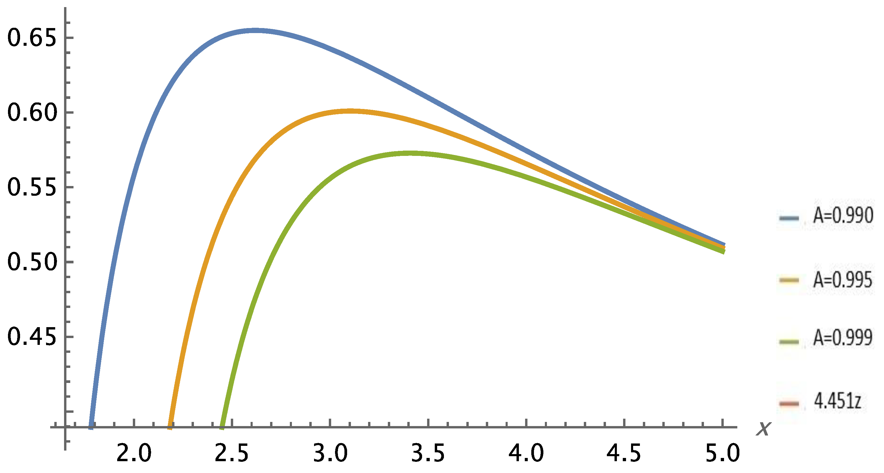
Figure 5.2.
The prediction of the distance of astronomical objects, in , for small values of redshift. Source: Figure by author.
Figure 5.2.
The prediction of the distance of astronomical objects, in , for small values of redshift. Source: Figure by author.
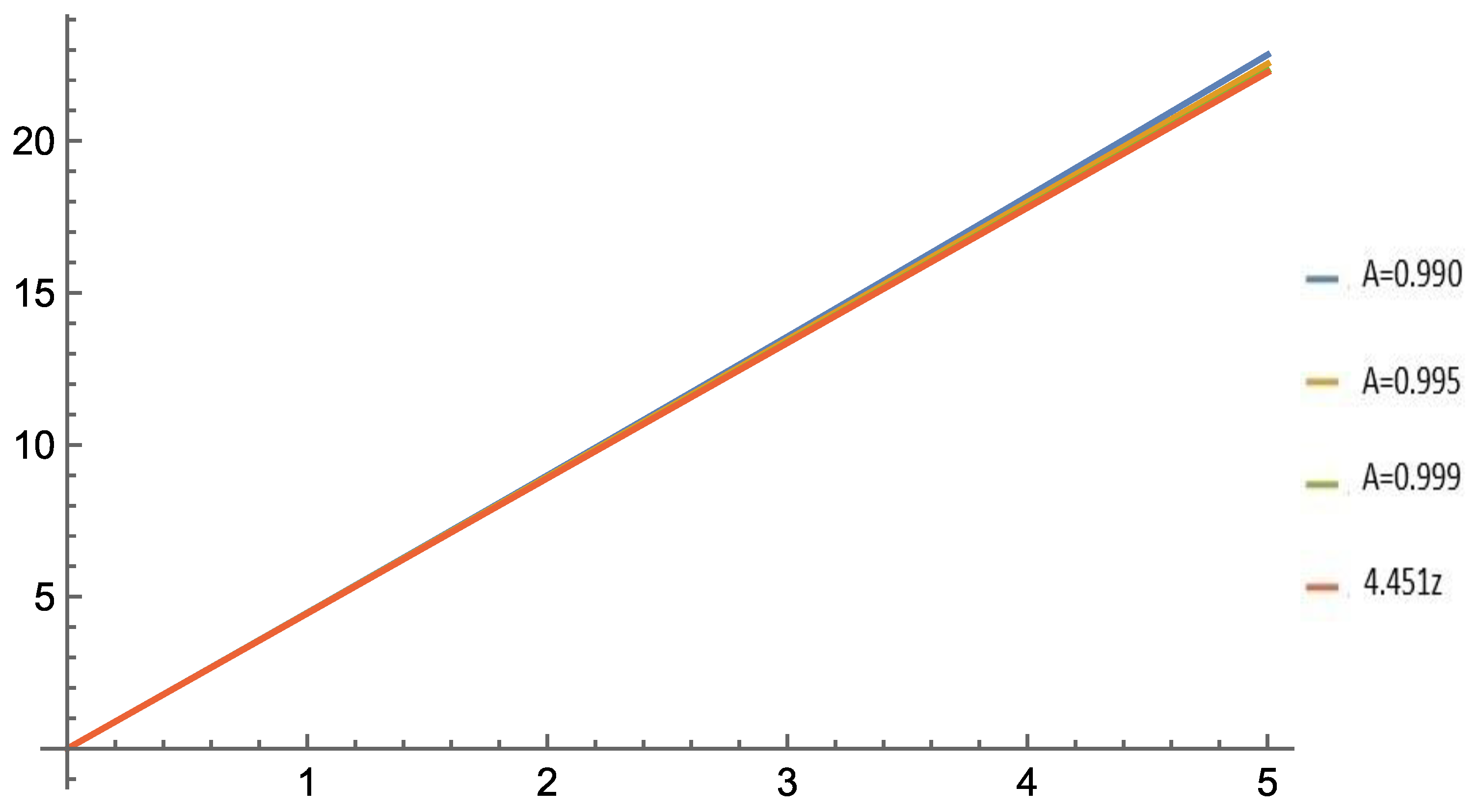
The Self-Variation Cosmological Model (SVCM) presents a fundamentally different approach to understanding the universe compared to the Standard Cosmological Model (SCM). While the SCM relies on the assumption of fixed physical constants and explains redshift through the expansion of space, the SVCM attributes redshift to the variation of particle properties—most notably the electron mass and charge—over cosmological time and distance.
This foundational shift allows the Self-Variation Theory to provide natural explanations for several longstanding issues in cosmology, such as:
The horizon problem, without invoking inflation;
The absence of magnetic monopoles, as a consequence of Maxwell's laws remaining valid under self-variation;
The flatness and uniformity of the universe;
The missing dark matter, by reproducing galactic rotation curves through its own gravitational equations;
The variation in the fine structure constant, as a direct prediction rather than an anomaly;
The Hubble tension, as a result of measuring cosmological parameters without accounting for the variation of particle masses.
Furthermore, the SVCM allows a smooth and continuous description of the universe’s evolution, starting from a "Vacuum State" rather than a singularity like the Big Bang. In contrast to the SCM, which reaches a theoretical breakdown at the singularity, the Self-Variation Theory extends beyond this point, providing a coherent framework that connects early-universe physics with present-day observations.
As astronomical instrumentation continues to advance, and deeper observations are made at higher redshifts, the Self-Variation Theory offers a testable and predictive model. Its potential to unify diverse phenomena under a single principle makes it a alternative to the current standard model of cosmology.
6. The Quantum Phenomena as a Consequence of the Self-Variation of Material Particles
In this Chapter we study the wave resulting from the propagation of self-variation as a perturbation in 4-dimensional spacetime. We calculate the wave function and apply it to the hydrogen and muon atoms. In the context of Self-Variation Theory, the time-independent Schrödinger Equation describes the self-variation of electric charge at the atomic scale.
We prove that the compatibility of the laws of physics with self-variation is equivalent to the use of the operators of quantum mechanics. The self-variation of material particles explains quantum phenomena.
We study the interaction of electric charges as an exchange of "information". Through the self-variation potential, information is transferred from the charge-source of the electromagnetic field to infinity. We briefly present the consequences of electric charge self-variation in this information.
6.1. The Propagation of Self-Variation as a Disturbance in Spacetime
Self-variation propagates as a "disturbance" in spacetime, i.e. it creates a wave. In the context of Self-Variation Theory, the wave created by the self-variation of the fundamental particles results in the quantum behavior of matter. Niels Bohr's work corresponds to a standing wave for which, however, we do not know the wave function [75]. Erwin Schrödinger understands the wave behavior of matter introduces the homonymous wave function, and applies the operators of quantum mechanics to a dynamical system, the hydrogen atom [82]. Werner Heisenberg introduces non-commutative matrices to quantum mechanics and formulates the uncertainty principle [80]. Paul Adrien Maurice Dirac combined quantum mechanics with Special Relativity in his work on the electron [77]. Richard Phillips Feynman gives a new interpretation to Dirac's conclusions, while through the homonymous diagrams he presents in a simple way the findings of electrodynamics [78,79]. To these leading physicists, and of course to Wolfgang Ernst Pauli [81] and Max Born [76], is due the enormous progress of quantum physics in a relatively short period of time. Quantum mechanics is the result of the work of many scientists. Since the first experiments in the mid-nineteenth century [83], the work of many distinguished physicists, both experimentally and theoretically, has brought quantum mechanics to the level we know it today.
The Self-Variation Theory requires that the mathematical form of the laws of physics be compatible with the principle of self-variation. This requirement places additional restrictions, than those set by the Theory of Relativity on the mathematical form of physical laws. In Chapters 3 and 4, we took into account that the potential is not uniquely defined and required it to be compatible with the self-variation principle. Thus we obtained the potential of the electromagnetic field, as given by the pairs of Equations (3.36) and (3.38) in the surrounding spacetime of a point electric charge. These potentials have different properties from potentials that do not take self-variation into account. One of these differences, the dependence of the second term of the potential on the acceleration of the field source, allows their application to the gravitational interaction as well. The consequences of self-variation are different on the point charge than in the surrounding spacetime. This difference initially expressed through Equations (3.20) and (3.59).
The self-variation in the surrounding spacetime of a point charge is given by Equation (3.20),
The self-variation electromagnetic potential is compatible with this Equation. The self-variation on the point charge is given by Equation (3.59),
The Liénard–Wiechert electromagnetic potential is compatible with this Equation. The laws of physics in both cases are compatible with self-variation. In the following Sections we present the consequences of self-variation on the point charge.
6.2. The Consequences of Self-Variation on the Point Charge
In this Section we study the generalized particle at the microscopic scale. At point in Figure 3.1 we consider a point electric charge interacting with the charge . We consider the case where the two charges are at a short distance, . Considering that in the inertial frame of reference where is stationary the emission of energy-momentum from in spacetime is isotropic we get,
Then, from the Lorentz-Einstein transformations we get,
, (6.1)
in an inertial frame of reference that moves with velocity . Equations (6.1) apply in the isotropic flat spacetime of Special relativity. Thus, in this Chapter we apply them to the electromagnetic interaction, as we studied it in Chapter 3. In a non-isotropic spacetime, Equations (6.1) do not apply. In Chapter 4 we saw that in interactions due to rest mass spacetime is not isotropic / flat. Therefore, to study the consequences of self-variation on the point rest mass, it is necessary to calculate the equation that replaces (6.1).
From Equations (6.1) and (1.1) we get,
. (6.2)
From these Equations we get,
. (6.3)
The effects of self-variation manifest differently at the location of the point charge compared to its surrounding spacetime. At the point charge itself, the propagation of self-variation as a spacetime perturbation is governed by Equation (6.3). In contrast, in the surrounding spacetime, the corresponding propagation is described by Equation (3.20),
. (6.4)
This distinction reflects the non-uniform distribution of energy–momentum and charge resulting from self-variation, and plays a central role in the formulation of the theory's field equations and potentials.
Through the substitution one Equation results from the other. However, and velocities have qualitative and quantitative differences. In the context of Special Relativity the velocity has constant measure in all inertial frames of reference. Velocity does not have this property. Also the inequality holds. Therefore, for any direction holds,
The Orbital Representation Theorem (refer to Section 3.5) gives an additional relation for the consequences of self-variation on the point charge and its surrounding spacetime. Within this context of information, the question arises to find the distance from the charge at which the self-variation passes from Equation (6.3) to Equation (6.4).
From Equations (1.1) and (6.3) we obtain,
. (6.5)
These Equations on the point charge are the counterparts of (3.79) and (3.81), which are valid in the surrounding spacetime of . We see that Equations (6.5) result from the pair of Equations (3.79), (3.81) by replacing the velocity with the velocity .
As a consequence of Equation (6.3), if the Liénard-Wiechert potentials are compatible with self-variation (refer to Equation (3.59)). Thus we have,
. (6.6)
From Equation (6.6) we get the potential energy of the system of the two charges,
. (6.7)
The charge density and the current density resulting from the self-variation of are given (refer to Appendix B) by the equations,
. (6.8)
The intensities of the electric field and the magnetic field are given by Equations (3.34) and (3.35) respectively. From Equations (6.3) and (6.8) we get,
and with equation we obtain,
. (6.9)
From Equations (6.9) we get,
. (6.10)
As we will see in Section 6.5, (6.10) expresses the continuity equation,
From Equation (6.3) we get,
. (6.11)
From Equation (6.11) and the first of Equations (6.2) we get,
. (6.12)
In quantum mechanics the partial derivatives are applied as operators, with the consequence that the second part of Equation (6.12) becomes zero. Applying the quantum mechanics operators to the Schrödinger wave function we get,
. (6.13)
Similarly we have,
. (6.14)
From Equations (6.13) and (6.14) we obtain,
. (6.15)
Equations (6.12) and (6.15) have the same form if the second part of Equation (6.12) is equal to zero. We will see the relation of quantum mechanical operators to self-variation in Section 6.4. Before that, in the next Section we will see the assumptions based on which the time-independent Schrödinger Equation is derived for hydrogen and muon atoms. The time-independent Schrödinger differential Equation is second order. Thus, for this study it is necessary to precede the following calculations.
From the first of the Equations (6.2) we get,
. (6.16)
Similarly, from the second of Equations (6.2) we obtain,
. (6.17)
At the microscopic scale the energy of a system of particles is taken constant, equal to its laboratory value. Thus, considering that the rest mass is independent of the self-variation of the electric field in Equations (6.16) and (6.17) we get,
, (6.18)
. (6.19)
Solving the system of Equations (6.18) and (6.19) we get the function . The solutions given by Equation (6.19) depend on the value of the constant , the velocity and its rate of change
In the next Section we apply Equation (6.19) to the hydrogen and muon atoms.
6.3. The Hydrogen and Muon Atoms
The conditions of the previous Section 6.3 hold for hydrogen and muon atoms. The accelerations of the electron and the muon respectively are due to their interaction only with the proton of the atom. If we now assume that the electron and muon velocities are non-relativistic, Equation (6.6) becomes,
. (6.20)
In this Equation the rest mass and the potential energy are treated as independent of the self-variation of the electric charge . For non-relativistic velocities , in Equation (6.7) substituting and where is the laboratory value of the charge of the electron in absolute value, we get,
. (6.21)
For non-relativistic velocities , from Equation (6.19) we get,
. (6.22)
Equation (6.22) gives periodic solutions if ,
. (6.23)
If we get the time-independent Schrödinger Equation,
. (6.24)
In the context of the Self-Variation Theory, the time-independent Schrödinger Equation expresses the self-variation of the electric charge, on the charge-carrier particle.
The differential Equation (6.24) gives the self-variation of the electric charge on the hydrogen and muon atoms. For more complete solutions it is required to avoid the approximations we have made. The difference of Equations (6.23) and (6.24) as well as the fact that the time-independent Schrödinger Equation is non-relativistic must be attributed to these approximations. We expect that investigation of the general Equation (6.17) will provide a more complete mathematical formalism for the hydrogen and muon atoms. An issue that has also not been explored is finding the conditions under which the self-variation of electron passes from Equation (6.3) to Equation (6.4) and vice versa.
The Equations of this Chapter are differentiated for individuals with an atomic number greater than 1. In the atom of helium there are interactions between the 4 electric charges. These interactions affect the inner product in Equation (6.23) and potential energy (6.7).
6.4. Quantum Mechanical Operators and Self-Variation
In this Section we study the relation of the individual derivatives in the equations of the Self-Variation Theory with the quantum mechanical operators,
. (6.25)
We first apply the operators (6.25)
. (6.26)
From Equation (3.34) we get,
. (6.27)
From Equations (6.26) and (6.27) we get,
, (6.28)
which are Equations (3.47).
The original proof that Maxwell's laws are compatible with self-variation was done in a different way (refer to Appendix B). From the comparison of the two proofs we arrive at the following conclusion: the compatibility of Maxwell's laws with self-variation is equivalent to the use of the operators (6.25) of quantum mechanics.
We now prove the continuity equation using the operators (6.25). First, from Equations (6.28) and we get,
. (6.29)
We apply the operators (6.25) to the continuity equation,
which is Equation (6.29). Working similarly, from Equation (6.29) we obtain the continuity equation. In the surrounding spacetime of a point electric charge, whether we apply Equations (3.6) - (3.29) or apply the operators (6.25) we get the same equations for the electromagnetic interaction.
We now apply the operators (6.25) and prove the continuity equation on the point charge . From Equation (6.10) we have,
Working similarly, from the continuity equation we obtain Equation (6.10).
The analysis presented in this section leads to the following fundamental conclusion:
The compatibility of the laws of physics with the principle of self-variation is mathematically equivalent to the use of the quantum mechanical operators defined in Equation (6.25).
This result emerges from a proof that involves two of the cornerstones of physics: Maxwell’s equations and the principle of charge conservation, as formulated through the continuity equation.
At the microscopic scale, the self-variation of material particles provides a natural explanation for the emergence of quantum phenomena. In this context, the appearance of quantum mechanical operators is not introduced axiomatically but arises as a direct consequence of the underlying self-variation dynamics. This connection offers a new theoretical foundation for quantum mechanics rooted in the physical process of self-variation.
6.5. The Rest Masses and
We now calculate the rest masses and . From Equation (2.6) we get,
. (6.30)
From Equation (2.6) we get,
. (6.31)
Equations (6.30) and (6.31) show the factors on which the rest masses and . One of these factors is the rate of change , i.e. the self-variation of the electric charge. If we ignore the self-variation by considering , from Equation (6.30) we get and from Equation (6.31) it follows that the rest mass is constant, . If from Equation (6.30) we have and from Equation (6.31) we have,
6.6. The Information in the Surrounding Spacetime of Electric Charge
The splitting of the electromagnetic potential of the self-variation into two individual potentials separates the electromagnetic field that accompanies the point electric charge in its motion, from the electromagnetic radiation it emits. Thus we have the possibility to do an analysis of the electromagnetic potential that cannot be done in the context of the classical Electromagnetic Theory.
At large distances from the electric charge the potential (3.36) tends to zero, and the electromagnetic potential is given by Equations (3.38),
. (6.32)
The potential (6.32) is independent of the distance (refer to Figure 3.1). From the first of Equations (6.32) we get the potential energy of the system of charges and ,
. (6.33)
An observer located at point measures the electric charge , where is the laboratory value of the charge of the electron, in absolute value. Thus, from Equation (6.33) we obtain,
. (6.34)
The potential given by Equation (6.33) is independent of distance, and therefore corresponds to a field with infinite range. This is consistent with the observed long-range behavior of electromagnetic radiation. Given the approximate charge neutrality of the universe—i.e., the existence of nearly equal amounts of positive and negative electric charge—the potential of Equation (6.33) does not contribute to the net energy content of the universe.
However, in the case of interaction between two electric charges, the potential of Equation (6.32) gives rise to an interaction energy described by Equation (6.33). For an observer located at a specific point in space, this energy is expressed explicitly by Equation (6.34). Through the mechanism of self-variation of the potential, a set of information is transmitted from the source of the electromagnetic field to infinity. Among these transmitted quantities is the self-variation of electric charge itself.
At distances down to the atomic scale, the variation in the value of interacting electric charges is governed by the equations of quantum mechanics. To a first approximation, Equation (6.24) provides a representative model for such variation. At these scales, a detailed analysis of the quantum mechanical framework can establish the limits within which the electric charge is allowed to vary.
Importantly, across all spatial scales, the electric charge does not act strictly with its constant, classical laboratory value, e. Instead, it undergoes a subtle process of self-variation. This has measurable implications for a broad range of physical processes, from photon exchange between charged particles to the dynamics of chemical reactions. When interpreted as an exchange of information, this self-variation introduces a statistical uncertainty—effectively, a margin of error—in the information carried by the interaction.
According to cosmological observations (see Section 5.2), the rate of this self-variation is extremely slow. Consequently, the associated probability of statistical error is expected to be correspondingly low—yet it remains non-zero.
6.7. The Interiority of the Universe in the Process of Measurement
The self-variation of material particles brings to the surface the interiority of the universe during the act of measurement. When measuring a physical quantity such as the electric charge , the unit of measurement itself is also subject to self-variation. This intrinsic variability cannot be directly observed in laboratory conditions; only its physical consequences can be measured. As a result, the question naturally arises: what mathematical formalism can adequately describe such a phenomenon?
At the microscopic scale, laboratory measurements suggest a periodic variation of the electric charge around its laboratory value . This periodic behavior emerges naturally from Equation (1.1), under the assumption that the constant , and is formally described by Equation (6.24). In this context, the laboratory value may be interpreted as a time-averaged representation of the electron’s electric charge. A possible connection between this self-variation and the Born statistical interpretation of the Schrödinger wave function remains an open question, meriting further investigation [76]. The Self-Variation Theory offers the foundational equations to support such an inquiry.
At cosmological distance scales, observations point to the effects of a genuine, distance-dependent variation in the value of the electric charge relative to its laboratory value. In this regime, the constant in Equation (1.1) is understood to be a real number, . In this way, the interiority of the universe—initially linked to the nature of observational apparatus—is reformulated as a purely mathematical matter: namely, the behavior of the parameter within the complex number set .
The profound relationship between mathematics and both art and science is continually reaffirmed within the mathematical formalism of physics. Bertrand Russell expressed this elegantly:
“Mathematics, rightly viewed, possesses not only truth, but supreme beauty-a beauty cold and austere, like that of sculpture, without appeal to any part of our weaker nature, without the gorgeous trappings of painting or music, yet sublimely pure, and capable of a stern perfection such as only the greatest art can show.”[111]
Yet, the application of mathematics in physics also requires a clearly defined conceptual framework within which its implications may be explored. In the present context, such a framework is provided by the three fundamental principles of the Self-Variation Theory.
The observable consequences of self-variation depend significantly on the spatial scale at which the phenomenon is examined. At microscopic distances, self-variation leads to an inherent uncertainty in measurements—arising from the variability of both the charge and the unit used to measure it. Charges never interact through their fixed laboratory values; rather, they exhibit a dynamic oscillation around these values.
At cosmological distances, the consequences of self-variation are directly imprinted in observational data. In fact, cosmological measurements represent the clearest and most anticipated manifestation of the phenomenon. At intermediate scales, one possible approach for probing the implications of self-variation is through the study of the self-variation potential itself.
Across all distance scales, the fundamental laws of physics appear to remain compatible with the self-variation of material particles.
Appendix A. Lorentz-Einstein Transformations of Physical Quantities and their Relations
In the 4-dimensional spacetime of Special Relativity, from Equations (1.15) we get,
. (A.1)
For the inertial reference system , from the first of Equations (A.1) we get,
Working in the same way in the rest of Equations (A.1), we finally get Equations (2.10) - (2.13).
Appendix B. Charge Density and Current Density in the Surrounding Spacetime of an Electric Point Charge. The Compatibility of Maxwell's Laws with Self-Variation
In Chapter 3, from Maxwell's first law we have proved Equation (3.47),
, (B.1)
for the charge density in the surrounding spacetime of the electric point charge . The current density in the surrounding spacetime of is calculated by Maxwell's fourth law,
. (B.2)
If we ignore self-variation and consider constant, at point there is no current density . Thus from Equations (B.2) and (3.48), (3.49) we get,
. (B.3)
Equation (B.3) is also proved using the auxiliary Equations (3.6) - (3.29). From Equations (B.2) and (3.34), (3.35) we get,
(refer to Equation (3.4), )
and
Maxwell's Equations are obviously compatible with Lorentz-Einstein transformations. We prove that they are also compatible with self-variance. Working similarly, as for the proof of Equations (3.47), for the second and third laws, we prove that Maxwell's laws are compatible with the self-variation of the point electric charge . The laws of physics are compatible with self-variation.
If we ignore self-variation and consider constant, from Maxwell's second law
. (B.4)
Equation (B.4) is also proved using the auxiliary Equations (3.6) - (3.29). From Equation (3.35) we get,
taking into consideration that the vector is perpendicular to the vectors and .
If we ignore self-variation and consider constant, from Maxwell's third law
. (B.5)
From Equations (3.34) and (3.35) we get,
Therefore, Maxwell's laws are compatible with the self-variation of point electric charge .
Appendix C. Second Way of Proving the Conservation of Electric Charge in the Surrounding Spacetime of a Point Charge
From the first of the Equations (3.47) we get
, (C.1)
where is the angle of the vectors and . For the volume of the sphere with center and radius (refer to Figure 3.1) we have,
. (C.2)
From Equations (C.1) and (C.2) we get,
. (C.3)
We denote
. (C.4)
Thus we have,
(C.5)
and
. (C.6)
So we have,
Appendix D. Proof of the Orbit Representation Theorem
In Figure 3.2, for the neighboring points
where
(D.1)
we have,
. (D.2)
For the time interval , during which the moved from point to point , we have
. (D.3)
From Equations (D.2) and (D.3) we get,
. (D.4)
From Equation (D.4) we get the tangent vector at point of the curve ,
. (D.5)
For the arc length of curve at point , from Equation (D.4) we obtain,
. (D.6)
For the curvature vector we have,
we obtain
. (D.7)
From Equation (D.7) we obtain,
. (D.8)
For the vector we have,
, (D.9)
if .
For the vector we have,
. (D.10)
From the third of Equations (3.60) we get,
. (D.11)
From Equations (3.62), (3.65), (3.67), (3.68), (3.66) and (3.69), by substituting
References
- Einstein, A. Die feldgleichungen der gravitation. Sitzungsberichte der Königlich Preußischen Akademie der Wissenschaften Berlin 1915, 844-847.
- Ohanian, H.C. Gravitation and Spacetime; W. W. Norton & Company Inc, New York, NY, USA, 1976.
- Schutz, B. F. A First Course in General Relativity; Cambridge University Press, Cambridge, New York, USA, 2009.
- Straumann, N. General Relativity and Relativistic Astrophysics; Springer, Berlin, Heidelberg, New York, 1984.
- Wald, R. M. General relativity; University of Chicago press, Chicago, USA, 1984.
- Manousos, E. Mass and charge selfvariation: A common underlying cause for quantum phenomena and cosmological data. Progress in Physics 2013, 3, 73-141.
- Manousos, E. Self-Variation Theory-Part I. International Journal of Physics, 2024, vol. 12, no. 4, 106-125. [CrossRef]
- Manousos, E. Self-Variation Theory-Part II. International Journal of Physics, 2024, vol. 12, no. 4, 126-146. [CrossRef]
- Liénard, A. Champ électrique et magnétique produit par une charge électrique concentrée en un point et animée d'un mouvement quelconque. G. Carré et C. Naud. 1898.
- Wiechert, E. Elektrodynamische elementargesetze. Annalen der Physik 1901, 309.4, 667-689. [CrossRef]
- Dodig, H. Direct derivation of Liénard–Wiechert potentials, Maxwell’s equations and Lorentz force from Coulomb’s law. Mathematics 2021, 9.3, 237. [CrossRef]
- Kühn, S. Inhomogeneous wave equation, Liénard-Wiechert potentials, and Hertzian dipoles in Weber electrodynamics. Electromagnetics 2022, 42.8, 571-593. [CrossRef]
- Plaja, L.; Enrique C. J. Introduction of the Liénard-Wiechert correction to the particle simulation of relativistic plasmas. Physical Review E 1998, 58.3, 3977. [CrossRef]
- Sebastian, J.; Mohammad Y. J.; Najmul H. Liénard-Wiechert potential of a heavy quarkonium moving in QGP medium. Physical Review D 2023, 107.5, 054040. [CrossRef]
- Christodoulides, Costas. The Special Theory of Relativity; Springer, New York, NY, USA, 2016. [CrossRef]
- Di Bartolo, B. Classical theory of electromagnetism; Prentice-Hall, Englewood Cliffs, New Jersey, NJ, USA, 1991.
- Einstein, A. On the electrodynamics of moving bodies. Annalen der Physik. 1905, 17 (10), 891-921.
- Faraoni, V. Special relativity; Springer Science & Business Media: Berlin/Heidelberg, Germany, 2013. [CrossRef]
- French, A. P. Special relativity; W. W. Norton & Company, New York, NY, USA, 1968.
- Gourgoulhon, E. Special relativity in general frames; Graduate Texts in Physics, Springer, New York, NY, USA, 2013. [CrossRef]
- Kruchinin, S. Problems and solutions in special relativity and electromagnetism; World Scientific Publishing Company, Singapore, 2017.
- Landau L. D.; Lifshitz, E. M. Mechanics and electrodynamics; Pergamon, Oxford, UK, 1972.
- Maxwell, J. C. II. A dynamical theory of the electromagnetic field. Proceedings of the Royal Society of London. 1864, 13, 531-536.
- Maxwell, J. C. VIII. A dynamical theory of the electromagnetic field. Philosophical transactions of the Royal Society of London. 1865, 155, 459-512. [CrossRef]
- Maxwell, J. C. On physical lines of force. Philosophical Magazine. 2010, 90, 11-23. [CrossRef]
- Resnick, R. Introduction to special relativity; Wiley: New York, NY, USA, 1968.
- Griffiths, D. J. Introduction to electrodynamics; 4th edn. Pearson Education, Boston, USA, 2013.
- Tsamparlis, Michael. Special relativity: An introduction with 200 problems and solutions; Springer, Heidelberg, Dordrecht, London, New York, 2010.
- Woodhouse, N. M. J. Special relativity; Springer, London, UK, 2003.
- Manousos, E. The replacement of the potentials as a consequence of the limitations set by the law of selfvariations on the rhysical laws. IJEIT 2014, 3.10, 181-185.
- Kenyon, I. R. Introduction to General Relativity and Cosmology (Second Edition); IOP Publishing, 2023.
- Corbelli, E.; Salucci, P. The extended rotation curve and the dark matter halo of M33. Monthly Notices of the Royal Astronomical Society. 2000, 311.2, 441-447. [CrossRef]
- Green, A. M.; Kavanagh, B. J. Primordial Black Holes as a dark matter candidate. Journal of Physics G: Nuclear and Particle Physics. 2021, 48.4, 043001. [CrossRef]
- Hong, S. E.; Jeong, D.; Hwang, H. S.; Kim, J. Revealing the local cosmic web from galaxies by deep learning. The Astrophysical Journal. 2021, 913.1, 76. [CrossRef]
- Manousos, E. Awaiting the Measurements by the James Webb Space Telescope: ‘A Hitherto Unrecognized Principle of Nature’ Justifies the Cosmological Data. European Journal of Applied Physics. 2023, 5.3, 31-35. [CrossRef]
- Najita, J. R.; Glenn P. T.; John S. C. From stars to superplanets: The low-mass initial mass function in the young cluster IC 348. The Astrophysical Journal. 2000, 541.2, 977. [CrossRef]
- Orkney, M. D.; Taylor, E.; Read, J. I.; Rey, M. P.; Pontzen, A.; Agertz, O.; Kim, S. Y.; Delorme, M. "EDGE: the shape of dark matter haloes in the faintest galaxies. Monthly Notices of the Royal Astronomical Society. 2023, 525.3, 3516-3532. [CrossRef]
- Quinn, T.; Parks, H.; Speake, C.; Davis, R. Improved determination of G using two methods. Physical review letters. 2013, 111.10, 101102. [CrossRef]
- Roberts, M. S.; Whitehurst, R. N. The rotation curve and geometry of M31 at large galactocentric distances. Astrophysical Journal. 1975, Vol. 201, p. 327-346 201, 327-346. [CrossRef]
- Rubin, V. C.; Ford, W. K. Jr; Thonnard, N. Rotational properties of 21 SC galaxies with a large range of luminosities and radii, from NGC 4605/R= 4kpc/to UGC 2885/R= 122 kpc. Astrophysical Journal, Part 1. 1980, vol. 238, 471-487.
- Taylor, A. N.; Dye, S.; Broadhurst, T. J.; Benitez, N.; Kampen, E. van. Gravitational Lens Magnification and the Mass of Abell 1689. The Astrophysical Journal 1998, 501 (2), 539–553. [CrossRef]
- Weijmans, A.-M.; Cappellari, M.; Bacon, R.; de Zeeuw, P. T.; Emsellem, E.; Falcón-Barroso, J.; Kuntschner, H.; McDermid, R. M.; van den Bosch, R. C. E.; van de Ven, G. Stellar Velocity Profiles and Line Strengths out to Four Effective Radii in the Early-Type Galaxies NGC 3379 and 821. Monthly Notices of the Royal Astronomical Society 2009, 398 (2), 561–574. [CrossRef]
- Yu, X.; Shi, Y.; Chen, Y.; Law, D. R.; Bizyaev, D.; Bing , L.; Li , S.; Zhou, L.; Chen, J.; Riffel, R. A.; et al. What drives the velocity dispersion of ionized gas in star-forming galaxies?. Monthly Notices of the Royal Astronomical Society. 2019, 486.4, 4463-4472. [CrossRef]
- Zwicky, Fritz. On the Masses of Nebulae and of Clusters of Nebulae. The Astrophysical Journal. 1937, 86, 217. [CrossRef]
- Bañados, E.; Venemans, B. P.; Mazzucchelli, C.; Farina, E. P.; Walter, F.; Wang, F.; Decarli, R.; Stern, D.; Fan, X.; Davies, F. B.; et al. An 800-million-solar-mass black hole in a significantly neutral Universe at a redshift of 7.5. Nature. 2018, 553.7689, 473. [CrossRef]
- Bowman, J. D.; Rogers, A. E.; Monsalve, R. A.; Mozdzen, T. J.; Mahesh, N. An absorption profile centred at 78 megahertz in the sky-averaged spectrum. Nature 2018, 555.7694, 67-70. [CrossRef]
- Cabrera, B. First results from a superconductive detector for moving magnetic monopoles. Physical Review Letters. 1982, 48.20, 1378. [CrossRef]
- Gott III, J. R.; Juric´, M.; Schlegel, D.; Hoyle, F.; Vogeley, M.; Tegmark, M.; Bahcall, N.; Brinkmann, J. A Map of the Universe. ApJ. 2005, Vol. 624, 463. [CrossRef]
- Guth, A. H. Inflationary universe: A possible solution to the horizon and flatness problems. Physical Review D. 1981, 23.2, 347. [CrossRef]
- Hubble, E.; Humason, M. L. The velocity-distance relation among extra-galactic nebulae. The Astrophysical Journal. 1931, 74, 43. [CrossRef]
- Kazanas, D. Dynamics of the universe and spontaneous symmetry breaking. Astrophysical Journal, Part 2-Letters to the Editor. 1980, vol. 241, Oct. 15, 241, L59-L63. [CrossRef]
- King, J. A.; Webb, J. K.; Murphy, M. T.; Flambaum, V. V.; Carswell, R. F.; Bainbridge, M. B.; Wilczynska, M. R.; Koch, F. E. Spatial variation in the fine-structure constant–new results from VLT/UVES. Monthly Notices of the Royal Astronomical Society. 2012, 422(4), 3370-3414. [CrossRef]
- Kirshner, R. P. Hubble's diagram and cosmic expansion. Proceedings of the National Academy of Sciences. 2004, 101.1, 8-13. [CrossRef]
- Kurt, V. G.; Shakhvorostova, N. N. CMB spectral distortions during the recombination of the primeval plasma in the early Universe. Physics-Uspekhi. 2014, 57.4, 389. [CrossRef]
- Lemaître, G. Univers homogène de masse constante et de rayon croissant rendant compte de la vitesse radiale des nébuleuses extra-galactiques. Annales de la Société Scientifique de Bruxelles. 1927, A47, 49-59.
- Manousos, E. Selfvariations vs Standard Cosmological Model Using as Criterion the Cosmological Data. GJSFR-A 2014, 14.2, 35-41.
- Manousos, E. The theory of self-variations. A continuous slight increase of the charges and the rest masses of the particles can explain the cosmological data. Nuovo Cimento B Serie. 2007, 122, 359-388.
- Manousos, E. Cosmological data could have a microscopic, not macroscopic, cause. American Journal of Space Science. 2013, 1, 10-21. [CrossRef]
- Manousos, E. On the absence of antimatter from the universe, dark matter, the fine structure parameter, the fluctuations of the cosmic microwave background radiation and the temperature difference between the northern and southern hemisphere of the universe. Physics International. 2013, 4.2, 120. [CrossRef]
- Manousos, E. The cause of the increased luminosity distances of supernovae recorded in the cosmological data. Progress in Physics. 2013, 15-16.
- Manousos, E. The numerical values of the fundamental parameters of the model of selfvariations and the age of the universe. Physics International. 2014, 5, 8-14. [CrossRef]
- Marrone, D. P.; Spilker, J. S.; Hayward, C. C.; Vieira, J. D.; Aravena, M.; Ashby, M. L. N.; Bayliss, M. B.; Béthermin, M.; Brodwin, M. ; Bothwell, M. S.; et al. Galaxy growth in a massive halo in the first billion years of cosmic history. Nature 2018, 553.7686, 51-54. [CrossRef]
- Natarajan, P.; Chadayammuri, U.; Jauzac, M.; Richard, J.; Kneib, J. P.; Ebeling, H.; Jiang, F.; van den Bosch, F.; Limousin, M.; Jullo, E.; et al. Mapping substructure in the HST Frontier Fields cluster lenses and in cosmological simulations. Monthly Notices of the Royal Astronomical Society. 2017, 468.2, 1962-1980. [CrossRef]
- Peacock, J. A.; Cole, S.; Norberg, P.; Baugh, C. M.; Bland-Hawthorn, J.; Bridges, T.; Cannon, R. D.; Colless, M.; Collins, C.; Couch, W.; et al. A measurement of the cosmological mass density from clustering in the 2dF Galaxy Redshift Survey. Nature 2001, 410.6825, 169-173. [CrossRef]
- Penzias, A. A.; Wilson, R. W. A Measurement of Excess Antenna Temperature at 4080 Mc/s. The Astrophysical Journal. 1965, 142, 419-421. [CrossRef]
- Perlmutter S.; Turner M.S.; White M. Constraining Dark Energy with Type Ia Supernovae and Large-Scale Structure. Physical Review Letters. 1999, 83, 670–673. [CrossRef]
- Riess, A. G.; Casertano, S.; Yuan, W.; Macri, L. M.; Scolnic, D. Large Magellanic Cloud Cepheid standards provide a 1% foundation for the determination of the Hubble constant and stronger evidence for physics beyond ΛCDM. The Astrophysical Journal. 2019, 876(1), 85. [CrossRef]
- Riess, A. G.; Filippenko, A. V.; Challis, P.; Clocchiatti, A.; Diercks, A.; Garnavich, P. M.; Gillilad, R.; Hogan, C. J.; Saurabh, J.; et al. Observational evidence from supernovae for an accelerating universe and a cosmological constant. The astronomical journal. 1998, 116.3, 1009. [CrossRef]
- Riess, A. G.; Anand, G. S.; Yuan 2, W.; Casertano, S.; Dolphin, A.; Macri, L. M.; Breuval, L.; Scolnic, D.; Perrin, M.; et al. JWST Observations Reject Unrecognized Crowding of Cepheid Photometry as an Explanation for the Hubble Tension at 8σ Confidence. The Astrophysical Journal Letters. 2024, 962.1, L17. [CrossRef]
- Slipher, V. M. The radial velocity of the Andromeda nebula. Popular Astronomy. 1914, vol. 22, 19-21.
- Tropp E. A.; Frenkel V. Y.; Chernin A. D. Alexander A. Friedmann: The Man Who Made the Universe Expand; Cambridge University Press, Cambridge, UK, 1993.
- Starobinsky, A. A. Robustness of the inflationary perturbation spectrum to trans-Planckian physics. Journal of Experimental and Theoretical Physics Letters. 2001, 73, 371-374. [CrossRef]
- Webb, J. K.; King, J. A.; Murphy, M. T.; Flambaum, V. V.; Carswell, R. F.; Bainbridge, M. B. Indications of a spatial variation of the fine structure constant. Physical Review Letters. 2011, 107.19, 191101. [CrossRef]
- Planck, M. On the law of distribution of energy in the normal spectrum. Annalen der Physik. 1901, 4 (553), 1.
- Bohr, N. XXXVII. On the constitution of atoms and molecules. The London, Edinburgh, and Dublin Philosophical Magazine and Journal of Science. 1913, 26.153, 476-502. [CrossRef]
- Born, M. Quantenmechanik der stoßvorgänge. Zeitschrift für physic. 1926, 38.11, 803-827. [CrossRef]
- Dirac, P. A. M. The quantum theory of the electron. Proceedings of the Royal Society of London. Series A, Containing Papers of a Mathematical and Physical Character. 1928, 118.779, 351-361. [CrossRef]
- Feynman, R. P. The theory of positrons. Quantum Electrodynamics. CRC Press, 2018, 167-177.
- Feynman, R. P. Space-time approach to quantum electrodynamics. Quantum Electrodynamics. CRC Press, 2018, 178-198.
- Heisenberg, W. Über den anschaulichen Inhalt der quantentheoretischen Kinematik und Mechanik. Zeitschrift für Physik. 1927, 43.3, 172-198. [CrossRef]
- Pauli, W. Über den Zusammenhang des Abschlusses der Elektronengruppen im Atom mit der Komplexstruktur der Spektren. Zeitschrift für Physik. 1925, 31.1, 765-783. [CrossRef]
- Schrödinger, E. Die Erfüllbarkeit der Relativitätsforderung in der klassischen Mechanik. Annalen der Physik. 1925, 382.11, 325-336.
- Planck, M. The genesis and present state of development of the quantum theory. Nobel Lecture. 1920, 2, 1–10.
- Álvarez-Rios I, Bernal T, Chavanis PH, Guzmán FS. Galactic rotation curves of low surface brightness galaxies using core-halo fuzzy dark matter configurations. Physical Review D. 2024, 110(063502). [CrossRef]
- Koop O, Antoja T, Helmi A, Callingham TM, Laporte CFP. Assessing the robustness of the Galactic rotation curve inferred from the Jeans equations using Gaia DR3 and cosmological simulations. Astronomy & Astrophysics. 2024, 692:A50. [CrossRef]
- Zhou Y, Li X, Huang Y, Zhang H. The Circular Velocity Curve of the Milky Way from 5–25 kpc Using Luminous Red Giant Branch Stars. Astrophysical Journal. 2023, 946(73). [CrossRef]
- Brown G, Rein H. General relativistic precession and the long-term stability of the Solar System. Mon Not R Astron Soc. 2023, 524(2):2046–2054. [CrossRef]
- Will CM. A new general relativistic contribution to Mercury’s perihelion advance. Phys Rev Lett. 2018, 120(19):191101. [CrossRef]
- Brown G, Rein H. General relativistic precession and the long-term stability of the Solar System. Mon Not R Astron Soc. 2023, 524(2):2046–2054.
- Will CM. A new general relativistic contribution to Mercury’s perihelion advance. Phys Rev Lett. 2018, 120(19):191101. [CrossRef]
- Lorenzo Iorio. Might the 2PN (second post-Newtonian) perihelion precession of Mercury become measurable in the next future? Universe. 2023, 9(1):37. [CrossRef]
- Park RS, Folkner WM, Konopliv AS, Williams JG, Smith DE, Zuber MT.
- Precession of Mercury’s Perihelion from Ranging to the MESSENGER Spacecraft. The Astronomical Journal. 2017, 153(3):121. [CrossRef]
- Dyson, F. W., Eddington, A. S., Davidson, C. A Determination of the Deflection of Light by the Sun’s Gravitational Field from Observations Made at the Total Eclipse of May 29, 1919. Philosophical Transactions of the Royal Society A. 1920, 220:291-333. [CrossRef]
- Fomalont E., Kopeikin S., Lanyi G., Benson J. Progress in Measurements of the Gravitational Bending of Radio Waves Using the VLBA. Astrophysical Journal. 2009, 699(2):1395. [CrossRef]
- Shapiro S. S., Davis J. L., Lebach D. E., Gregory J. S. Measurement of the Solar Gravitational Deflection of Radio Waves using Geodetic VLBI Data, 1979-1999. Phys Rev Lett. 2004, 92:121101. [CrossRef]
- Shapiro II. Fourth test of general relativity. Phys Rev Lett. 1964 Dec 28;13(26):789-91. [CrossRef]
- De Blok WJG, Walter F, Brinks E, Trachternach C, Oh SH, Kennicutt RC. High-resolution rotation curves and galaxy mass models from THINGS. Astron J. 2008, 136(6):2648. [CrossRef]
- Corbelli, E.; Salucci, P. The extended rotation curve and the dark matter halo of M33. Monthly Notices of the Royal Astronomical Society. 2000, 311.2, 441-447. [CrossRef]
- Green, A. M.; Kavanagh, B. J. Primordial Black Holes as a dark matter candidate. Journal of Physics G: Nuclear and Particle Physics. 2021, 48.4, 043001. [CrossRef]
- Martinsson TP, Verheijen MA, Westfall KB, Bershady MA, Andersen DR, Swaters RA. The DiskMass Survey-VII. The distribution of luminous and dark matter in spiral galaxies. Astron Astrophys. 2013, 557:A131. [CrossRef]
- Shankaranarayanan S, Lubo M. Gauge-invariant perturbation theory for trans-Planckian inflation. Phys Rev D. 2005, 72(12):123513. [CrossRef]
- Curti M, Witstok J, Jakobsen P, Kobayashi C, Curtis-Lake E, Carniani S, et al. JADES: The star-formation and chemical enrichment history of a luminous galaxy at z ~ 9.43 probed by ultra-deep JWST/NIRSpec spectroscopy. Mon Not R Astron Soc. 2024, 530(1):1–19. [CrossRef]
- Hsiao TYY, Álvarez-Márquez J, Coe D, Crespo Gómez A, Brammer G, Mahler G, et al. JWST MIRI Detections of Hα and [O III] and a Direct Metallicity Measurement of the z = 10.17 Lensed Galaxy MACS0647-JD. Astrophys J Lett. 2023, 957(1):L4. [CrossRef]
- Larson RL, Finkelstein SL, Kocevski DD, Bagley M, Ferguson HC, Giavalisco M, et al. A CEERS Discovery of an Accreting Supermassive Black Hole 570 Myr after the Big Bang: Identifying a Progenitor of Massive z > 6 Quasars. Astrophys J Lett. 2023, 951(1):L15. [CrossRef]
- Sandage, Al. Edwin Hubble 1889-1953. Journal of the Royal Astronomical Society of Canada. 1989, Vol. 83, NO. 6/DEC, 351.
- Price, P. B.; Shirk, E. K.; Osborne, W. Z.; Pinsky, L. S. Evidence for detection of a moving magnetic monopole. Physical Review Letters. 1975, 35.8, 487. [CrossRef]
- Alpher, R. A.; Herman, R. Evolution of the Universe. Nature 1948, 162.4124, 774-775. [CrossRef]
- Ijjas, A.; Steinhardt, P. J.; Loeb, A. Inflationary schism. Physics Letters B. 2014, 736, 142-146. [CrossRef]
- Gamow, G. The evolution of the universe. Nature 1948, 162.4122, 680-682. [CrossRef]
- Rindler, Wolfgang. Relativity: special, general, and cosmological.; OUP Oxford, 2006. [CrossRef]
- Russell, Bertrand. The basic writings of Bertrand Russell; Simon and Schuster, New York, NY, USA, 1961.
Disclaimer/Publisher’s Note: The statements, opinions and data contained in all publications are solely those of the individual author(s) and contributor(s) and not of MDPI and/or the editor(s). MDPI and/or the editor(s) disclaim responsibility for any injury to people or property resulting from any ideas, methods, instructions or products referred to in the content. |
© 2025 by the authors. Licensee MDPI, Basel, Switzerland. This article is an open access article distributed under the terms and conditions of the Creative Commons Attribution (CC BY) license (http://creativecommons.org/licenses/by/4.0/).
Copyright: This open access article is published under a Creative Commons CC BY 4.0 license, which permit the free download, distribution, and reuse, provided that the author and preprint are cited in any reuse.


