
Submitted:
29 September 2025
Posted:
30 September 2025
You are already at the latest version
Abstract
Bud break is a critical phenological stage in muscadine grapevines, marking the start of the growing season and the increasing need for irrigation management. Real-time bud detection enables irrigation to match muscadine grape phenology, conserving water and enhancing performance. This study presents BudCAM, a low-cost, solar-powered, edge-computing camera system based on Raspberry Pi 5 and integrated with LoRa radio board, developed for real-time bud detection. Nine BudCAMs were deployed at Florida A&M University Center for Viticulture and Samll Fruit Research from mid February to mid March, 2024, monitoring three wine cultivars (A-27, noble, and Floriana) with three replicates each. Muscadine grape canopy images were captured every 20 minutes between 7:00 to 19:00, generating 2656 high-resolution (4656×3456 pixels) bud break images as database for bud detection algorithm development. The dataset was divided into 70% training, 15% validation, and 15% test. YOLOv11 models were trained using two primary strategies: a direct single-stage detector on tiled raw images and a refined two-stage pipeline that first identifies the grapevine cordon. Extensive evaluation of multiple model configurations identified top performers for both the single-stage (mAP@0.5=86.0%) and two-stage (mAP@0.5=85.0%) approaches. Further analysis revealed that preserving image scale via tiling was superior to alternative inference strategies like resizing or slicing. Field evaluations during the 2025 growing season confirmed the system’s effectiveness, with the two-stage model showing greater robustness to environmental noise like lens fog. A time-series filter smooths the raw daily counts to reveal a clear phenological trend for visualization. In its final deployment, the autonomous BudCAM system captures an image, runs inference on-device, and transmits the bud count in under three minutes, demonstrating a complete, field-ready solution for precision vineyard management.
Keywords:
Bud break detection
; Object detection
; YOLOv11
; Muscadine vineyard management
; Deep learning
1. Introduction
Bud break represents a critical phenological stage in grapevines, marking the beginning of each new growing season and influencing both vegetative development and fruit set. In muscadine grape production, irrigation is particularly important during the first two years while vines are establishing, and after establishment, water requirements are greatest from bud-break through flowering [1]. Adequate soil water availability is essential during bud break and early shoot growth, as water stress at this stage can restrict vegetative expansion, resulting in smaller canopies and reduced grape yield and quality [1]. Bud break serves not only as a vital phenological indicator but also as a practical signal for initiating irrigation in grapevine management.
Bud break monitoring in commercial vineyards largely depends on manual visual inspection. Vineyard growers typically record bud break timing, extent, and progression by scouting rows and visually counting buds, which is time-consuming, labor-intensive, and prone to subjectivity. The reliance on manual methods restricts monitoring efforts to small sample areas, limiting decision-making and the ability to optimize vineyard management at scale. Furthermore, bud break is highly sensitive to environmental conditions, particularly spring temperature [2], making timely and accurate monitoring even more essential.
To address these limitations, recent advances in computer vision and deep learning have provided powerful tools for automating agricultural tasks. Deep learning models, which use large numbers of parameters to recognize complex patterns, have become widely applied in computer vision. One key task is object detection, which identifies and labels objects within images by drawing bounding boxes around them [3]. This approach can be adapted for agriculture, where cameras capture field images and the system detects buds among grapevines [4,5,6], supporting more efficient field monitoring.
Grimm et al. [7] proposed a Convolutional Neural Network (CNN)-based semantic segmentation approach that localizes the grapevine organs at the pixel scale and then counts them via connected-component labeling. Similarly, Rudolph et al. [8] used a CNN-based segmentation model to identify inflorescence pixels and then applied a circular Hough Transform to detect and count individual flowers. Marset et al. [9] proposed a Fully Convolutional Network (FCN)-MobileNet that directly segments grapevine buds at the pixel level and benchmarked it against a strong sliding-window patch-classifier baseline [10], reporting better segmentation, correspondence, and localization. Xia et al. [6] introduced Attention-guided data enrichment network for fine-grained classification of apple bud types, using a Split-Attention Residual Network (ResNeSt-50) [11] backbone with attention-guided CutMix and erasing modules to focus learning on salient bud regions.
Beyond pixel-wise segmentation, single-stage detectors such as the You Only Look Once (YOLO) family are popular in agriculture vision due to the excellent speed-performance tradeoff and suitability for edge devices. Common strategies for low-power deployment include lightweight backbone (e.g., GhostNet [12]), depthwise separable convolutions [13], attention modules such as the Bottleneck Attention Module (BAM) [14]), enhanced multi-scale fusion, and modern Intersection over Union (IoU) losses. Li et al. [4] proposed a lightweight YOLOv4 for tea bud detection by replacing the backbone with the GhostNet and introducing depthwise separable convolutions [13] to reduce parameters and floating-point operations per second (FLOPS), stabilized bounding boxes regression of small buds in clutter with Scaled Intersection over Union (SIoU) [15]. Gui et al. [5] compressed YOLOv5 using GhostConv with BAM and weighted feature fusion in the neck, retaining Complete Intersection over Union (CIoU) [16] for regression. Chen et al. [17] introduced TSP-YOLO for monitoring of cabbage seedlings emergence, modifying YOLOv8-n by replacing C2f with Swin-conv [18] for stronger multi-scale features and adding ParNet attention [19] to suppress background clutter. Pawikhum et al. [20] used YOLOv8-n for apple bud detection and aggregated detections over time downstream to avoid double counts and omissions. Taken together, these studies illustrate a consistent recipe for small-object detection on resource-constrained platforms.
Within this design space, YOLOv11 [21] offered architectural updates targeted at small-object detection under field conditions while maintaining low latency for edge deployment. The C3k2 block replaced the C2f in the backbone and neck, improving computational efficiency, and the addition of a C2PSA spatial-attention block enhances the model’s ability to focus on salient regions, which is critical for detecting small buds against complex background. Reported benchmarks indicate YOLOv11 attains comparable or improved accuracy with fewer parameters than prior YOLO versions, achieving similar mean Average Precision (mAP@0.5) with 22% fewer parameters than YOLOv8. These properties align with the needs of a low-power, in-field bud-monitoring system.
This study develops custom-built bud detection camera (BudCAM), an integrated, low-cost, solar-powered edge-computing system for automated bud break monitoring. The objectives of this study are to:
- (1)
- deploy the BudCAM devices for in-field data acquisition and on-device processing;
- (2)
- develop and validate YOLOv11-based detection framework on bud break image database images built in 2024 and 2025; and
- (3)
- establish a post-processing pipeline that converts raw detections into a smoothed time-series for phenological analysis.
Collectively, these contributions advance automated, edge-based monitoring of grapevine bud development.
2. Materials and Methods
This section begins with an overview of the BudCAM hardware, a description of field sites, and the data collection strategy, which together form the foundation for deploying bud break detection algorithms on the custom-built camera in field applications. The BudCAM units captured images at regular intervals during the bud break period, and these images were annotated to create training datasets for YOLOv11 detection models. Different image processing strategies, model configurations, and data augmentation methods were evaluated to determine optimal performance. Model accuracy was assessed through multiple testing strategies and validated under real-world field conditions.
2.1. Hardware Development
BudCAM is mounted one meter above the grapevine to capture images of the canopy (Figure 1). The grapevine cordon is positioned approximately 1.5 m above the ground. BudCAM is mounted 1 m above the cordon to capture images of the canopy, resulting in a total camera height of about 2.5 m from the ground.
The BudCAM system integrates multiple hardware components into a low-cost, solar-powered, edge-computing platform designed for field deployment in vineyards. A Raspberry Pi 5, equipped with a 512 GB SD card, serves as the central processing unit, managing image capture, local execution of the trained deep learning model, and data transmission. The ArduCAM 16 MP autofocus camera captures high-resolution (4656×3456 pixels) grapevine canopy images, ensuring sharp focus for bud detection and clear visualization. The BudCAM is powered by two 3.7V, 11,000 mAh lithium batteries connected in parallel to meet the demand of the Raspberry Pi 5 during inference. This configuration is necessary because a single battery cannot supply sufficient current when BudCAM executes the object detection algorithm. The two batteries are charged by a 6 V, 20 W solar panel via a voltage regulator that conditions the panel output and regulates constant current/constant voltage (CC/CV) charging. Power delivery to the Raspberry Pi 5 is managed by a PiJuice HAT power management board, which features a Real-Time Clock (RTC) to automatically wake the system at 30-minute sampling intervals during daylight hours (07:00–19:00), thereby optimizing energy use. The BudCAM follows a three-step processing framework (Figure 2): (1) image acquisition and on-device processing by the Raspberry Pi 5, (2) transmission of processed bud counts via a Maduino LoRa radio board (915 MHz) to a custom-built Raspberry Pi 4 LoRa gateway, and (3) cloud-based visualization through a dedicated web interface1. Due to LoRa’s limited bandwidth, only per-image bud count is transmitted, while raw images remain stored locally on the SD card for offline analysis. The gateway, located within LoRa range at a powered site (e.g., laboratory), pushes the data via the internet to the cloud server for visualization, enabling real-time vineyard monitoring through the web platform.
2.2. Experiment Site and Data Collection
This experiment was conducted at the Center for Viticulture and Small Fruit Research at Florida A&M University during 2024 and 2025 muscadine grape growing season. Nine muscadine grapevines representing three cultivars (Floriana, Noble, and A27) were monitored, with three vines randomly selected as replicates for each cultivar. Each vine was equipped with a dedicated BudCAM unit. During the 2024 growing season, nine BudCAMs operated continuously from March to August (Table 1), capturing images every 20 minutes between 07:00 to 19:00 daily. Images were collected throughout the growing season, but only those captured during each vine’s specific bud break period were selected for algorithm development. These bud break periods varied by grapevine, ranging from late March to mid-April, as detailed in Table 1. The selected images were manually annotated for bud detection using the Roboflow platform [22]. In this study, distinguishing between buds and shoots was particularly difficult from top-view images, where the structures often overlap and appear visually similar. To maintain consistency, we combined both categories under a single label, “bud,” during dataset annotation. This simplified the process while still capturing the key developmental stages required for monitoring grapevine growth. In 2025, the nine BudCAMs were deployed to test the bud detection algorithm developed from 2024 data. During the 2025 field testing and validation period (March 5 to April 20), the systems automatically processed images using the trained model every 30 minutes between 7:00 and 19:00 daily.
2.3. Software Development for BudCAM
2.3.1. Detection Algorithm
The detection framework was implemented using the YOLOv11 [21], developed by Ultralytics in PyTorch and publicly available. YOLOv11 comprises three main components: the backbone, the neck, and the head (Figure 3). The backbone extracts multi-scale features, which are then aggregated and refined by the neck. The head uses these refined features to predict bounding-box coordinates, class probabilities, and confidence scores for bud detection [21].
Two approaches were employed for both training and inference:
- (1)
- Single-Stage Bud Detector: A YOLO model was trained directly to detect buds from images, outputting bounding boxes and confidence scores for each detected bud (Figure 4(a)).
- (2)
- Two-Stage Pipeline: A grapevine cordon detection model first identifies the main grapevine structure. When a cordon prediction exceeds a confidence threshold, the corresponding region is cropped from the original image and passed to a second YOLO model trained specifically for bud detection. Images where no cordon meets the confidence threshold are skipped to avoid false detection from non-vine area (Figure 4(b)).
Both detection approaches process images using a tiling strategy rather than directly analyzing full-resolution images, with details provided in Section 2.3.2. After detecting buds in each tile, each bud detection with its bounding box is mapped back to the original-image coordinates for evaluation and bud count.
2.3.2. Dataset Preparation
A total of 2656 high-resolution (4656×3456 pixels) raw images were collected in 2024 as bud break image database and split into 70% for training, 15% for validation, and 15% for test subsets. The distribution of raw images per vine across these three subsets is provided in Table 2, which ensures balanced representation of cultivars for model development and evaluation. From these subsets, two derived datasets were prepared using different processing strategies: the Raw Grid (RG) dataset and the Cordon-Cropped (CC) dataset. The RG dataset feeds the single-stage pipeline, whereas the CC dataset is used in the two-stage pipeline as input to the second-stage bud detector. CC images were generated by applying a separately trained cordon detector to crop the cordon region, which was then used for bud detection.
The first strategy tiled each raw image into 6×4 grid (776×864 pixels per tile), forming the RG dataset (Table 3). The CC dataset was generated in two steps. First, a cordon detector was trained using a YOLOv11-medium model on 1500 annotated cordon images resized to 1280×1280 pixels, with augmentation including flips and rotations up to 180°. The model was fine-tuned from COCO-pretrained weights for 500 epochs with a batch size of 32. It achieved an mAP@0.5 of 0.99 and an mAP@0.95 of 0.86, ensuring reliable extraction of the cordon region. Using this detector, the grapevine cordon was cropped from each image and then tiled into 640×640 patches. These patches formed the CC dataset, which was specifically used to train the bud detector. The relationship between the two dataset preparation strategies and their role in the pipelines is summarized in Table 3.
Both of the RG and CC datasets consist of training, validation and test subsets derived respectively from the same divisions of the raw images. Image tiling for both datasets was performed after annotation, and annotations were exported in YOLO format [23]. To reduce false positives and improve generalization, background-only tiles were retained so that approximately 80% of the training tiles contained visible buds. The number of samples in each subset for the RG and CC datasets is summarized in Table 3. For CC dataset generation, the cordon detector applied a confidence threshold of 0.712 (selected by maximizing F1 on the validation set). The highest-scoring cordon above threshold was cropped, whereas images without a cordon above threshold were excluded from the CC dataset.
2.3.3. Model Training Configuration
Several training configurations were evaluated to assess model performance, including the application of transfer learning, augmentation hyperparameter tuning, and model size variation. All configurations were trained on two NVIDIA Tesla V100 GPUs (32 GB each) at Holland Computing Center (HCC) at the University of Nebraska-Lincoln.
Transfer learning was implemented by initializing models with weights pretrained on the COCO dataset [24], allowing them to converge faster and leverage knowledge learned from the source task and be fine-tuned for the target task. Data augmentation was performed on-the-fly during training, ensuring that augmented samples differed across epochs to enhance dataset diversity and model generalization. Two augmentation configurations were evaluated, with parameters randomly sampled from uniform distributions, and details are provided in Table 4.
Configuration 1 followed the setup by Marset et al. [9], representing a commonly used augmentation scheme in object detection studies. Each raw sample was augmented by (1) rotation from 0° to 45°, (2) horizontal and vertical translation up to 0.4, (3) scaling between 0.7 and 1.3, (4) shearing up to 0.1, and (5) horizontal and vertical flips. Configuration 2 was derived from Configuration 1 to better reflect the small bud size in the images and BudCAM’s deployment, which captures a top-down view of the cordon and buds. A mild perspective transformation was added to account for foreshortening, while translation, scaling, and shear ranges were reduced to avoid excessive distortion of small buds. The rotation range was narrowed from 45° to 10° to prevent angular distortion and bounding-box misalignment. These modifications reflect a trade-off between robustness to spatial variation and preserving bud visibility, critical for tiny-object detection. To investigate the effect of model capacity, the large model variant was also tested alongside the medium model.
Eight training configurations (Models 1–8; Table 5) were defined by combining augmentation setup, transfer learning, and model size. Each configuration was applied to both the RG and CC datasets, producing 16 trained models in total. For the two-stage pipeline, the CC-trained models served as the bud detector, while the cordon detector was trained separately as a preprocessing step.
All input samples were resized to 640×640 pixels using bilinear interpolation [25] to match the input size requirement of YOLOv11. Training was conducted with a batch size of 128 using the stochastic gradient descent (SGD) optimizer, an initial learning rate of 0.01 scheduled by cosine annealing, and a maximum of 1000 epochs. Early stopping was applied, with training terminated if the validation metric failed to improve for 20 consecutive epochs. To assess robustness, each configuration was repeated five times with different random seeds. Model performance was evaluated using mean Average Precision (mAP) at an Intersection over Union (IoU) threshold of 0.5, a standard metric in object detection that measures the agreement between predicted bounding boxes and ground-truth annotations.
2.3.4. Inference Strategies on the 2024 Dataset
Model performance was first evaluated using the baseline test set, where predictions were generated directly from prepared test set without additional processing. To more thoroughly investigate the performance under different conditions, two additional inference strategies were applied. In both strategies, the grapevine cordon region was first extracted from the raw test images using the pre-trained cordon detector, and the cropped regions were then processed as follows:
- (1)
- Resized Cordon Crop test set (Resize-CC): Each cropped cordon region was resized to the model’s 640×640 input size. This approach tests how well the model handles significant downscaling, where tiny objects like buds risk losing critical detail.
- (2)
- Sliced Cordon Crop evaluation (Sliced-CC): Although the baseline tiling strategy is effective, it may split buds located at tile boundaries, which can result in missed detections. This Sliced-CC strategy was therefore evaluated as an alternative to solve this "object fragmentation" problem. It was achieved using a sliding-window technique. Each cordon crop was divided into 640×640 slices with a slice-overlap ratio r (r = 0.2, 0.5, and 0.75). After the model processed each slice individually, the resulting detections were remapped to the original image coordinates and merged using non-maximum suppression (NMS).
2.4. Setup of Real-World Testing
The trained models were deployed on nine BudCAMs during the 2025 muscadine grapevine growing season at Florida A&M University Center for Viticulture and Small Fruit Research to evaluate near–real-time monitoring and data acquisition. Two types of visual evaluation were conducted: offline evaluations provided qualitative detection results across models, while online evaluations demonstrated real-world performance under field conditions. The offline evaluation used all images collected between March 5 and April 20, 2025, across nine posts, and was conducted using the optimal single-stage model (the one with the highest mAP@0.5 among Models 1–8) and the optimal two-stage model (the one with the highest mAP@0.5 among Models 1–8). The online evaluation continuously reported near–real-time detection results from YOLOv11-Medium (Model 7 of single-stage) deployed on BudCAM. Processed outputs were displayed on a custom-designed website2, demonstrating the edge-computing capability of the system. This field evaluation captured dynamic conditions such as changing sunlight, camera angles, and bud growth stages, providing a realistic assessment of model performance in practice.
2.5. Time-Series Post-Processing
Bud counts from the nine posts were ordered by timestamp to generate a raw time series for each vine. The raw data, however, contains spurious fluctuations due to transient imaging artifacts, such as lens fogging, glare, exposure flicker. To reduce this noise and produce a continuous representation of the biological trend, an adaptive Exponentially Weighted Moving Average (adaptive-EWMA) smoother [26] was applied to down-weight outliers and reduce misleading spikes in the plots. Let denote the observed bud count and the previous smoothed value for . The adaptive-EWMA updates as:
where is Huber clipping function,
where is the residual, which represents how much the current observation deviates from the expected (smoothed) value . The Huber function treats small residuals proportionally, but clips large residuals. This prevents extreme observations from disproportionately influencing the smoothed series. In this study, was defined as twice the robust standard deviation:
where MAD is the median absolute deviation. The constant is the standard consistency factor that makes MAD a robust estimator of under Gaussian distributions [27,28,29]. The smoothing parameter was determined by the effective window size [30]:
Since bud count trend were expected to vary on a daily scale, and with 22 images captured per day, was set to 22, yielding . These settings were used to generate the smoothed time-series curves.
3. Results and Discussion
This section presents the evaluation of the trained models, organized into three parts. The baseline performance of all 16 model configurations, including eight trained on the RG dataset and eight trained on the CC dataset, was first compared to examine the effects of model size, fine-tuning, and data augmentation, which led to the selection of the two best models (Table 4, Table 5). Secondly, these top models were evaluated with alternative inference strategies (Resized-CC and Sliced-CC) to determine the most effective processing approach. Finally, the performance of the selected models was illustrated with qualitative examples from the 2024 dataset, capturing both early and full bud break to confirm model robustness, compared with related work, and evaluated through a quantitative time-series analysis of 2025 field images.
3.1. Model Performance and Inference Strategy Evaluation
The comparison between medium-size models (Model 1 and Model 2) and large-size models (Model 3 and Model 4) showed only marginal differences across both datasets (Table 6). In the RG dataset, the fine-tuned medium model (Model 2, mAP@0.5 = 80.3%) outperformed the fine-tuned large model (Model 4, mAP@0.5 = 78.5%) by 1.8%, while in the CC dataset, medium and large models achieved nearly identical accuracy (79.1–79.2% without fine-tuning and 78.3–78.7% with fine-tuning). These findings indicate that increasing model size didn’t lead to meaningful improvements in bud detection accuracy, and the medium-size models are preferable for deployment, where comparable detection accuracy can be achieved with faster inference speed on edge devices like Raspberry Pi 5.
The effect of fine-tuning on model performance was inconsistent (Table 6). For example, in the RG dataset, fine-tuning improved accuracy in the medium model, with Model 2 (80.3%) outperforming Model 1 (75.9%) by 4.4%. However, in augmented models the effect was minimal, with Model 6 (85.3%) only slightly higher than Model 5 (85.1%). Similarly, in the CC dataset, Model 8 (85.0%) performed nearly the same as Model 7 (84.7%). Overall, fine-tuning reduced training duration due to earlier convergence but did not consistently enhance model accuracy.
Data augmentation proved to be an effective training factor (Table 6). In the RG dataset, for instance, the fine-tuned model with augmentation (Model 6, mAP@0.5=85.3%) significantly outperformed its counterpart without augmentation (Model 2, mAP@0.5=80.3%), by 5-point mAP@0.5 improvement. A similar gain was also observed in the CC dataset, where the fine-tuned model with augmentation (Model 8, mAP@0.5 = 85.0%) exceeded the non-augmented fine-tuned model (Model 2, mAP@0.5 = 78.3%) by 6.7%.Similar improvements were observed across all comparisons, confirming the benefits of augmentation for enhancing model accuracy.
Based on these comparisons, two best-performing models—RG-trained Model 7 and CC-trained Model 8——were selected for evaluation using alternative inference strategies, including Resized-CC and Sliced-CC applied to the original 4K-resolution images, which described in Section 2.4. In this extended evaluation, both models under Resized-CC and Sliced-CC settings showed reduced performance compared to the baseline (Table 7). This performance gap can be explained by differences in how the datasets were prepared. The training data for Models 7 (RG) and 8 (CC) were derived from grids or patches cropped from 4K-resolution images, which preserved sufficient detail for detecting small buds. By contrast, the Resized-CC dataset was produced directly by scaling entire 4K images down to 640×640 pixels. This downscaling reduced the bud size for reliably detection, thereby substantially degrading performance. Consequently, Model 7 dropped from 86.0% mAP@0.5 (baseline) to 58.2% under Resized-CC, while Model 8 decreased from 85.0% to 52.6% (Table 7).
In contrast to the Resized-CC results, the Sliced-CC evaluation produced reduced performance even though this strategy was expected to improve detection by leveraging overlapping regions. A likely explanation is an increase in false positives. Specifically, each model performed 24 predictions per image when evaluated on the RG test set, corresponding to the 6×4 grid of tiles. With slice prediction and nonzero overlap, even more patches were generated per image, leading to redundant predictions and thus more false positives. To further investigate this trend, two higher overlap ratios (0.5 and 0.75) were tested. As shown in Table 8, detection accuracy consistently declined as the overlap ratio increased. For Model 7 (RG), mAP@0.5 decreased from 74.8% at r=0.2 to 72.0% at r=0.5 and further to 66.3% at r=0.75. A similar trend was observed for Model 8 (CC), where mAP@0.5 dropped from 80.0% at r=0.2 to 76.4% at r=0.5 and 69.2% at r=0.75. These results support the hypothesis that excessive prediction redundancy from overlapping slices increases false positives, and degrade overall performance.
Based on these results, the original, scale-preserving tiling procedures were confirmed as the optimal inference strategies. Therefore, the following two configurations were used for all subsequent analyses:
- (1)
- RG-trained Model 7, used with pre-processing step that tiles each raw image into a 6×4 grid.
- (2)
- CC-trained Model 8, used within the two-stage pipeline where a cropped cordon region is tiled into 640×640 patches for bud detection.
These approaches were applied consistently to analyze the test set images and the field images from the 2025 growing season.
3.2. Dataset Comparison and 2024 Processed Image Examples
Two raw images from each cultivar were selected—one captured representing the early bud break season and the other during the full bud break season—resulting in six raw images in total. Detection confidence thresholds were determined from the optimal F1 scores on the respective validation sets: 0.279 for RG-trained Model 7 and 0.369 for CC-trained Model 8. Each image was processed using RG-trained Model 7 and CC-trained Model 8, and the inference results are presented in Figure 5 and Figure 6. Both models successfully detect buds in both early- or full-season conditions. Notably, the selected examples include images captured at different times of the day (morning, midday, evening), demonstrating that both models remain robust under varying lighting conditions.
3.3. Comparison with Related Methods
The recent studies on bud, flower, and seedling detection or segmentation are summarized in Table 9. Although datasets, viewpoints, and evaluation metrics differ substantially, segmentation studies often report F1 scores, whereas detection frameworks typically use mAP@0.5. Even with these differences, the comparison provides perspective on relative performance. Most prior works (Table 9) appear to have been tested on servers or workstations, as the platform was not specified. Only Pawikhum et al. and our work have reported embedded/edge inference. BudCAM is distinctive for achieving on-device detection on a Raspberry Pi 5 with mAP@0.5 values above 0.85, demonstrating that accuracy competitive with previous studies can be maintained while enabling practical and low-cost field applications.
3.4. Real-World Inference in 2025
RG-trained Model 7 and CC-trained Model 8 were further applied to perform inference on images captured between March 5 and April 20, 2025, aligning with the bud season. The raw and smoothed bud counts are shown in Figure 7 and Figure 8.
Analysis of the RG-trained results (Figure 7) shows substantial noise, including severe outliers inconsistent with the early stage of bud break. For example, vine NP6 registered an anomalous peak count of 51 on March 14, 2025, near the onset of bud break. This outliers were influential enough to bias the adaptive-EWMA smoother, pulling the smoothed value up to 49 in this case. This indicates that while the smoother attenuates minor fluctuations, it can be compromised by large, persistent false positives. Inspection of corresponding images (Figure 9) suggests that most anomalies resulted from false detections caused by lens fogging in the early morning.
In contrast, the CC-trained results (Figure 8) exhibit fewer such anomalies, and all nine plots show the expected increase in bud count over time. The improvement stems from the cordon-detection stage, which filters out frames where a cordon cannot be confidently localized, reducing the likelihood that fogged-lens images proceed to bud detection. The adaptive-EWMA smoother was applied to stabilize residual variability at the day scale. Nevertheless, some noise remains (e.g., vine NP2 around April 10, 2025). Review of the corresponding images, CC-trained Model 8 underperformed in certain conditions (Figure 10), such as relatively dark images or those affected by rainbow lens flare. In these cases, buds were under-detected, and occasionally entirely missed (e.g., the left panel of Figure 10). The failure is likely because such poor-quality images were excluded during dataset preparation, leaving the model insufficiently trained to generalize to these unseen scenarios, especially when buds appear small relative to the overall image. This underestimation contributes to sharp downward excursions especially late in the season where isolated frames drop to zero or near-zero while adjacent frames report typical counts (10-40).
Finally, to illustrate the deployed system, Figure 11 shows the dashboard view for vine NP6, plotting raw counts at 30-minute intervals over March-April, 2025. In addition, the BudCAM requires approximately three minutes to complete a full operational cycle, including waking from sleep, capturing and processing an image, transmitting the bud count, and returning to sleep.
4. Conclusions
Bud break marks the transition from dormancy to active growth, when grapevine water requirements increase sharply. Near real-time bud detection provides critical information for irrigation decision-making by aligning water applications with the actual phenological stage of muscadine grape. To address this need, this work introduced BudCAM, a low-cost, solar-powered edge-computing system designed to provide near real-time bud monitoring in muscadine vineyards at 30-minute intervals. This study evaluated 16 YOLOv11 model configurations across two distinct approaches: a single-stage detector using a Raw Grid (RG) dataset and a two-stage pipeline using a Cordon-Cropped (CC) dataset.
The top models from each approach, RG-trained Model 7 (mAP@0.5=86.0%) and CC-trained Model 8 (mAP@0.5=85.0%), were evaluated against alternative inference strategies (Resized-CC and Sliced-CC). This analysis confirmed that the original, scale-preserving tiling methods were superior, highlighting that preserving bud scale is critical for accurate detection. In field evaluations using data collected during the 2025 muscadine grape growing season at Florida A&M University Center for , the CC-trained two-stage model showed greater robustness to environmental noise like lens fog, though its performance was reduced in challenging lighting conditions such as dark scenes or glare.
Taken together, these results indicate that reliable, on-device bud detection is now feasible at field scale. By applying time-series smoothing to filter noise from the raw daily counts, the BudCAM system enables growers to track bud break progression and align early-season irrigation with phenological demand. Future work should prioritize improving model robustness to challenging lighting conditions and enhancing generalization across different sites and cultivars.
Acknowledgments
This work is supported by the Agriculture and Food Research Initiative Competitive Grants Program, Foundational and Applied Science, project award no. 2023-69017-40560, from the U.S. Department of Agriculture’s National Institute of Food and Agriculture, and by the U.S. National Science Foundation Experiential Learning for Emerging and Novel Technologies (ExLENT) Program (award no. 2322535). The authors also thank Philipine Andjawo for assistance with data labeling and curation.
References
- Hickey, C.C.; Smith, E.D.; Cao, S.; Conner, P. Muscadine (Vitis rotundifolia Michx., syn. Muscandinia rotundifolia (Michx.) Small): The resilient, native grape of the southeastern US. Agriculture 2019, 9, 131. [Google Scholar] [CrossRef]
- Reta, K.; Netzer, Y.; Lazarovitch, N.; Fait, A. Canopy management practices in warm environment vineyards to improve grape yield and quality in a changing climate. A review A vademecum to vine canopy management under the challenge of global warming. Scientia Horticulturae 2025, 341, 113998. [Google Scholar] [CrossRef]
- Zhang, H.; Li, F.; Liu, S.; Zhang, L.; Su, H.; Zhu, J.; Ni, L.M.; Shum, H.Y. Dino: Detr with improved denoising anchor boxes for end-to-end object detection. arXiv preprint arXiv:2203.03605, arXiv:2203.03605 2022.
- Li, J.; Li, J.; Zhao, X.; Su, X.; Wu, W. Lightweight detection networks for tea bud on complex agricultural environment via improved YOLO v4. Computers and Electronics in Agriculture 2023, 211, 107955. [Google Scholar] [CrossRef]
- Gui, Z.; Chen, J.; Li, Y.; Chen, Z.; Wu, C.; Dong, C. A lightweight tea bud detection model based on Yolov5. Computers and Electronics in Agriculture 2023, 205, 107636. [Google Scholar] [CrossRef]
- Xia, X.; Chai, X.; Zhang, N.; Sun, T. Visual classification of apple bud-types via attention-guided data enrichment network. Computers and Electronics in Agriculture 2021, 191, 106504. [Google Scholar] [CrossRef]
- Grimm, J.; Herzog, K.; Rist, F.; Kicherer, A.; Toepfer, R.; Steinhage, V. An adaptable approach to automated visual detection of plant organs with applications in grapevine breeding. Biosystems Engineering 2019, 183, 170–183. [Google Scholar] [CrossRef]
- Rudolph, R.; Herzog, K.; Töpfer, R.; Steinhage, V.; et al. Efficient identification, localization and quantification of grapevine inflorescences and flowers in unprepared field images using Fully Convolutional Networks. Vitis 2019, 58, 95–104. [Google Scholar]
- Marset, W.V.; Pérez, D.S.; Díaz, C.A.; Bromberg, F. Towards practical 2D grapevine bud detection with fully convolutional networks. Computers and Electronics in Agriculture 2021, 182, 105947. [Google Scholar] [CrossRef]
- Pérez, D.S.; Bromberg, F.; Diaz, C.A. Image classification for detection of winter grapevine buds in natural conditions using scale-invariant features transform, bag of features and support vector machines. Computers and electronics in agriculture 2017, 135, 81–95. [Google Scholar] [CrossRef]
- Zhang, H.; Wu, C.; Zhang, Z.; Zhu, Y.; Lin, H.; Zhang, Z.; Sun, Y.; He, T.; Mueller, J.; Manmatha, R.; et al. networks. In Proceedings of the Proceedings of the IEEE/CVF conference on computer vision and pattern recognition, 2022, pp.
- Khanam, R.; Hussain, M. What is YOLOv5: A deep look into the internal features of the popular object detector. arXiv preprint arXiv:2407.20892, arXiv:2407.20892 2024.
- Howard, A.G.; Zhu, M.; Chen, B.; Kalenichenko, D.; Wang, W.; Weyand, T.; Andreetto, M.; Adam, H. Mobilenets: Efficient convolutional neural networks for mobile vision applications. arXiv preprint arXiv:1704.04861, arXiv:1704.04861 2017.
- Park, J.; Woo, S.; Lee, J.Y.; Kweon, I.S. Bam: Bottleneck attention module. arXiv preprint arXiv:1807.06514, arXiv:1807.06514 2018.
- Gevorgyan, Z. SIoU loss: More powerful learning for bounding box regression. arXiv preprint arXiv:2205.12740, arXiv:2205.12740 2022.
- Zheng, Z.; Wang, P.; Ren, D.; Liu, W.; Ye, R.; Hu, Q.; Zuo, W. Enhancing geometric factors in model learning and inference for object detection and instance segmentation. IEEE transactions on cybernetics 2021, 52, 8574–8586. [Google Scholar] [CrossRef] [PubMed]
- Chen, X.; Liu, T.; Han, K.; Jin, X.; Wang, J.; Kong, X.; Yu, J. TSP-yolo-based deep learning method for monitoring cabbage seedling emergence. European Journal of Agronomy 2024, 157, 127191. [Google Scholar] [CrossRef]
- Liu, Z.; Lin, Y.; Cao, Y.; Hu, H.; Wei, Y.; Zhang, Z.; Lin, S.; Guo, B. Swin transformer: Hierarchical vision transformer using shifted windows. In Proceedings of the Proceedings of the IEEE/CVF international conference on computer vision, 2021, pp.
- Goyal, A.; Bochkovskiy, A.; Deng, J.; Koltun, V. Non-deep networks. Advances in neural information processing systems 2022, 35, 6789–6801. [Google Scholar]
- Pawikhum, K.; Yang, Y.; He, L.; Heinemann, P. Development of a Machine vision system for apple bud thinning in precision crop load management. Computers and Electronics in Agriculture 2025, 236, 110479. [Google Scholar] [CrossRef]
- Khanam, R.; Hussain, M. Yolov11: An overview of the key architectural enhancements. arXiv preprint arXiv:2410.17725, arXiv:2410.17725 2024.
- Roboflow. Roboflow, 2025.
- Redmon, J.; Divvala, S.; Girshick, R.; Farhadi, A. You only look once: Unified, real-time object detection. In Proceedings of the Proceedings of the IEEE conference on computer vision and pattern recognition, 2016, pp.
- Liang, W.z.; Oboamah, J.; Qiao, X.; Ge, Y.; Harveson, B.; Rudnick, D.R.; Wang, J.; Yang, H.; Gradiz, A. CanopyCAM–an edge-computing sensing unit for continuous measurement of canopy cover percentage of dry edible beans. Computers and Electronics in Agriculture 2023, 204, 107498. [Google Scholar] [CrossRef]
- Press, W.H. Numerical recipes 3rd edition: The art of scientific computing; Cambridge university press, 2007.
- Zaman, B.; Lee, M.H.; Riaz, M.; Abujiya, M.R. An adaptive approach to EWMA dispersion chart using Huber and Tukey functions. Quality and Reliability Engineering International 2019, 35, 1542–1581. [Google Scholar] [CrossRef]
- Huber, P.J. Robust statistics. In International encyclopedia of statistical science; Springer, 2011; pp. 1248–1251.
- Rousseeuw, P.J.; Croux, C. Alternatives to the median absolute deviation. Journal of the American Statistical association 1993, 88, 1273–1283. [Google Scholar] [CrossRef]
- Leys, C.; Ley, C.; Klein, O.; Bernard, P.; Licata, L. Detecting outliers: Do not use standard deviation around the mean, use absolute deviation around the median. Journal of experimental social psychology 2013, 49, 764–766. [Google Scholar] [CrossRef]
- Brown, R.G. Smoothing, forecasting and prediction of discrete time series; Courier Corporation, 2004.
| 1 | |
| 2 |
Figure 1.
(Left): Illustration of BudCAM deployed in the research vineyard at Florida A&M University Center for Viticulture and Small Fruit Research. (Right): Components of BudCAM include: (1) ArduCAM 16MP autofocus camera, (2) Maduino LoRa radio board, (3) two 3.7V lithium batteries, (4) Raspberry pi 5 and PiJuice power management board, (5) LoRa antenna, (6) voltage regulator, and (7) solar cable.
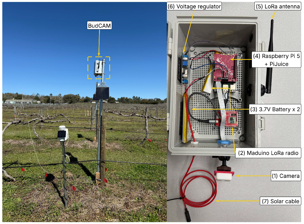
Figure 2.
Overview of three-phase processing framework for developing BudCAM.
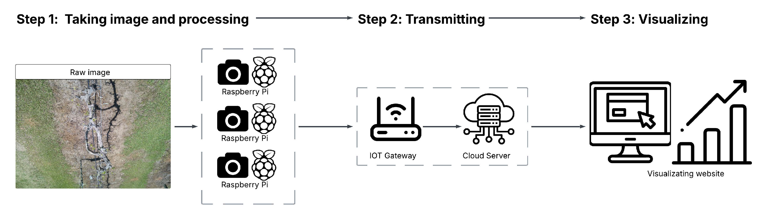
Figure 3.
Architecture of YOLOv11 used in BudCAM. The network comprises a backbone that extracts multi-scale features, a neck that aggregates/refines these features, and a detection head that predicts bounding box coordinates , and a confidence score from tiled inputs.
Figure 3.
Architecture of YOLOv11 used in BudCAM. The network comprises a backbone that extracts multi-scale features, a neck that aggregates/refines these features, and a detection head that predicts bounding box coordinates , and a confidence score from tiled inputs.
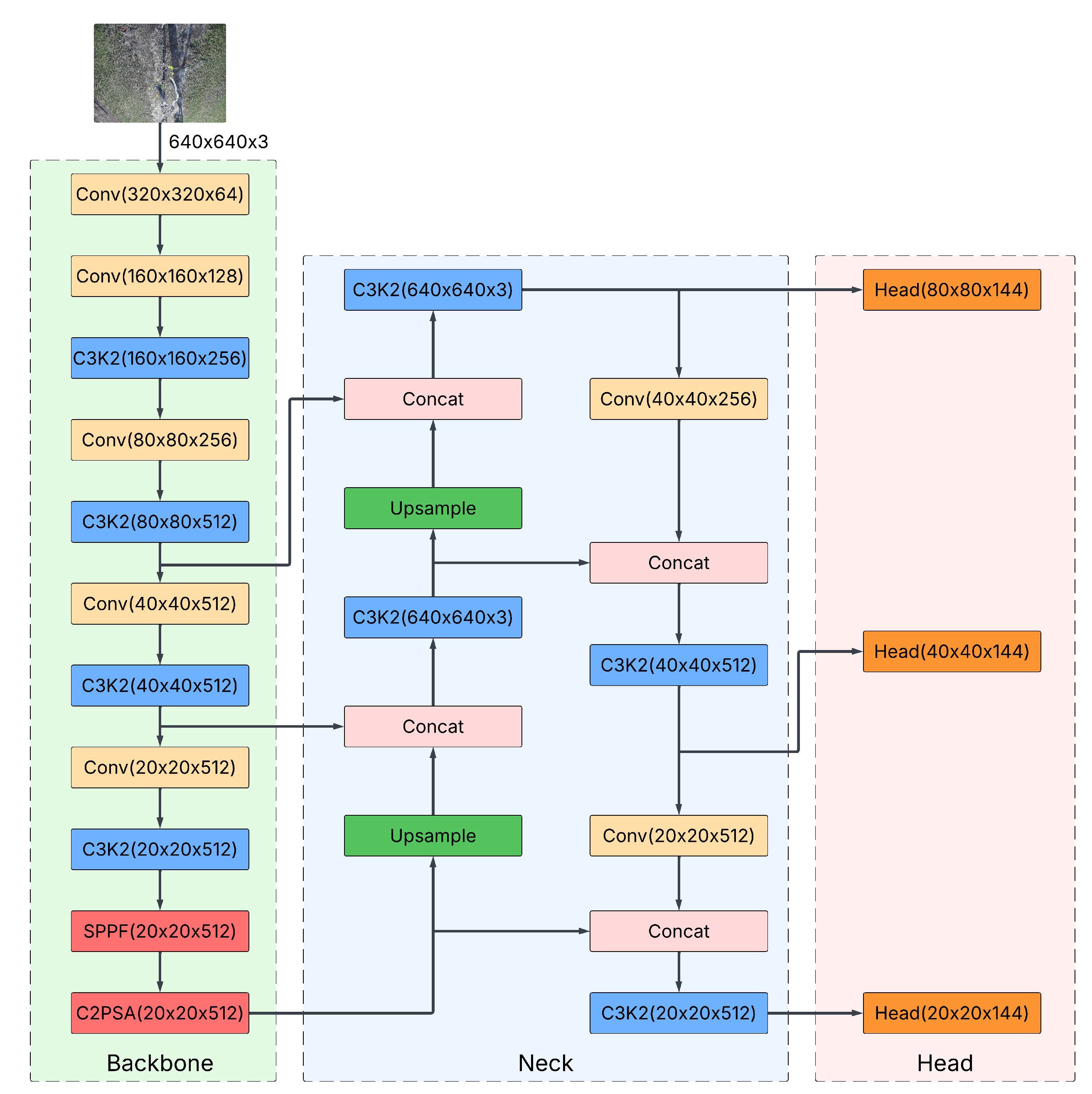
Figure 4.
Comparison of the two detection pipelines. (a) Single-stage bud detector: the raw image is divided into a 6×4 grid (tiles of 776×864 pixels); each tile is processed by a YOLOv11 bud detector. Tile-level detections are mapped back to the full image and merged to obtain the final bud counts. (b) Two-stage pipeline: a YOLOv11 cordon detector first localizes the grapevine cordon, which is then cropped and partitioned into 640×640 px patches. These patches are processed by a second YOLOv11 model, and the results are merged. In all panels, detected buds are shown in red and the detected cordon is shown in blue.
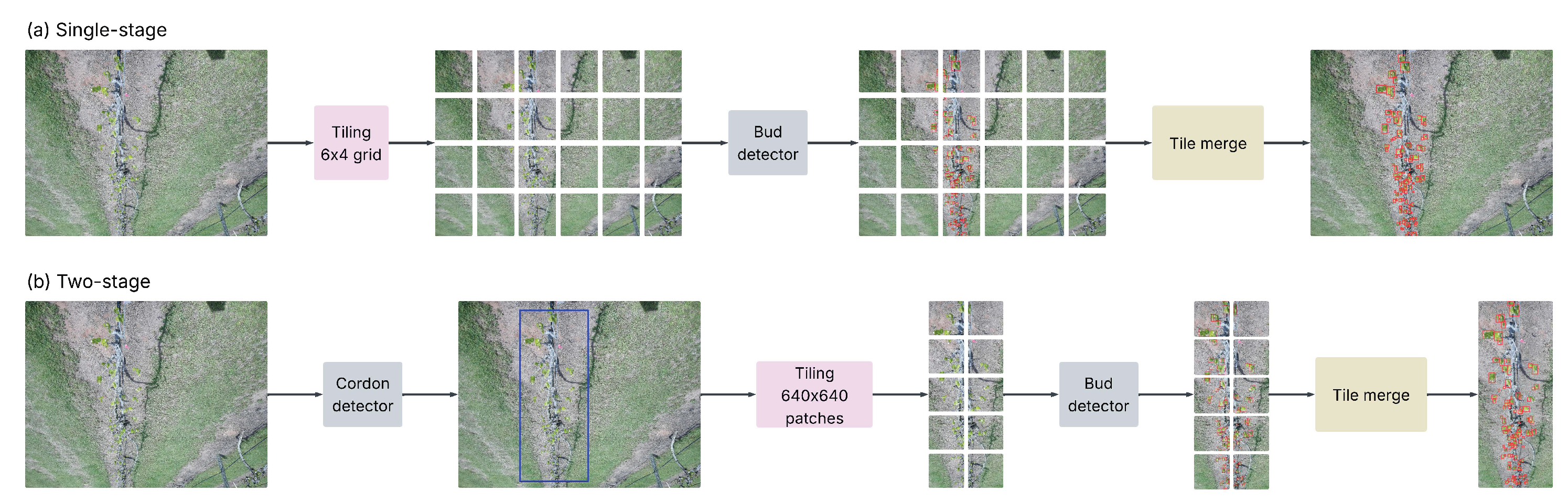
Figure 5.
Images from three cultivars captured in the early bud break season, with inference results from RG-trained Model 7 and CC-trained Model 8. Column 1: raw images with ground-truth buds (pink bounding boxes) and total bud counts; the capture time is marked in the top-left corner of each image. Column 2: inference results from Model 7 showing detected buds (red bounding boxes with confidence scores). Column 3: inference results from Model 8, where the blue bounding box indicates the cordon region identified by the cordon detector, and red bounding boxes mark detected buds with confidence scores. Bud counts in Columns 2 and 3 represent the total detections per image.
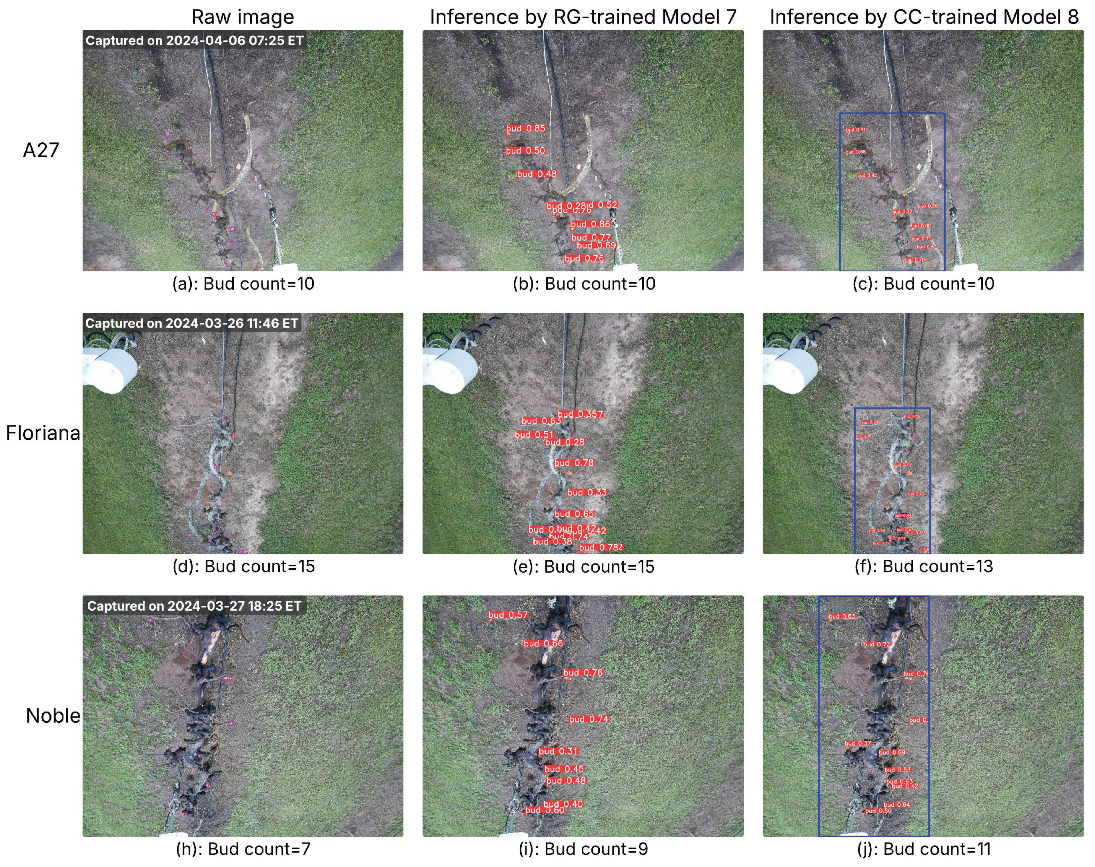
Figure 6.
Images from three cultivars captured in the full bud break season, with inference results from RG-trained Model 7 and CC-trained Model 8. Layout and labeling follow the same convention as Figure 5.
Figure 6.
Images from three cultivars captured in the full bud break season, with inference results from RG-trained Model 7 and CC-trained Model 8. Layout and labeling follow the same convention as Figure 5.
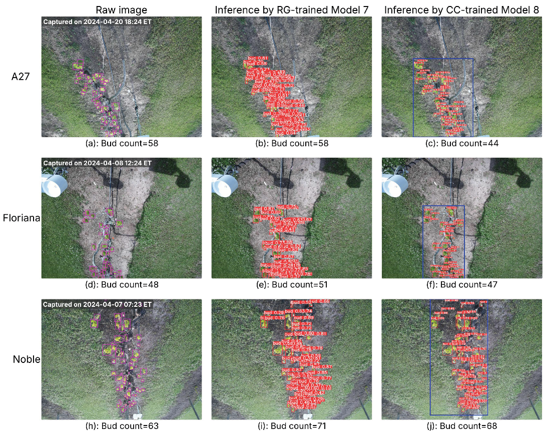
Figure 7.
Inference results from RG-trained Model 7. Black dots represent the raw bud counts and red dots represent the smoothed values obtained by adaptive-EWMA.
Figure 7.
Inference results from RG-trained Model 7. Black dots represent the raw bud counts and red dots represent the smoothed values obtained by adaptive-EWMA.
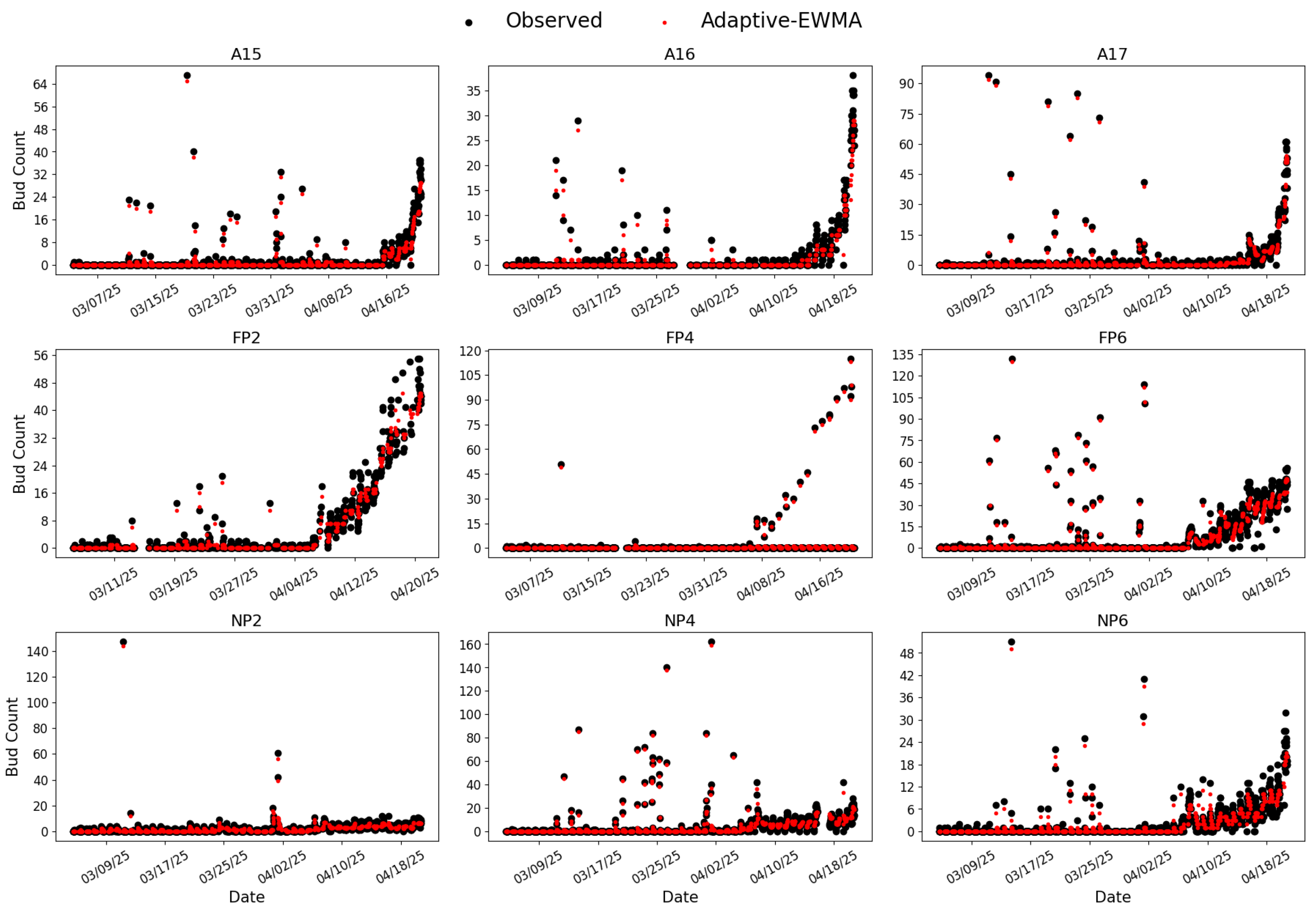
Figure 8.
Inference results from CC-trained Model 8. Labeling follows the same convention as Figure 7.
Figure 8.
Inference results from CC-trained Model 8. Labeling follows the same convention as Figure 7.
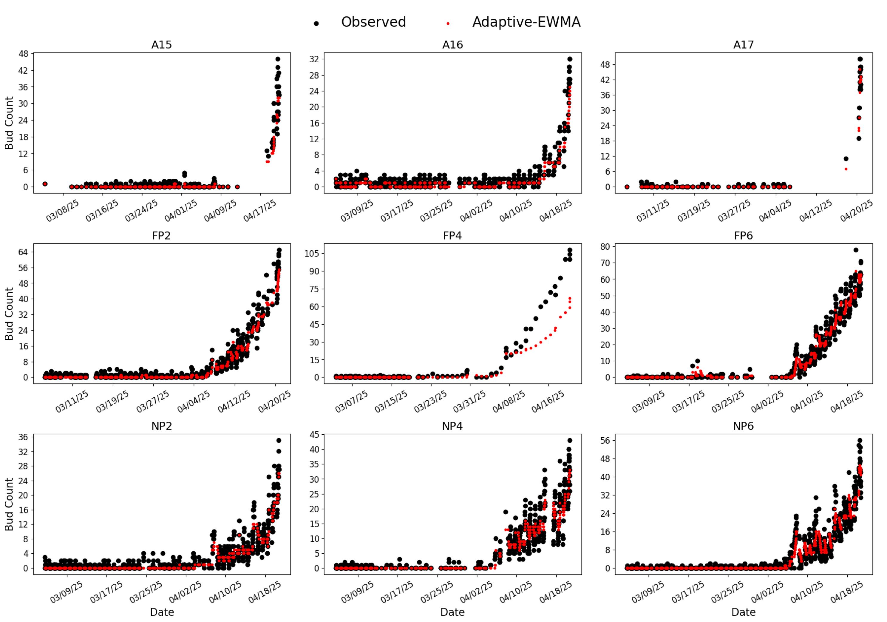
Figure 9.
Example images of three cultivars captured with a fogged lens and processed by RG-trained Model 7. Detected buds are highlighted with red bounding boxes. The capture time is shown in the top-left corner of each image.
Figure 9.
Example images of three cultivars captured with a fogged lens and processed by RG-trained Model 7. Detected buds are highlighted with red bounding boxes. The capture time is shown in the top-left corner of each image.
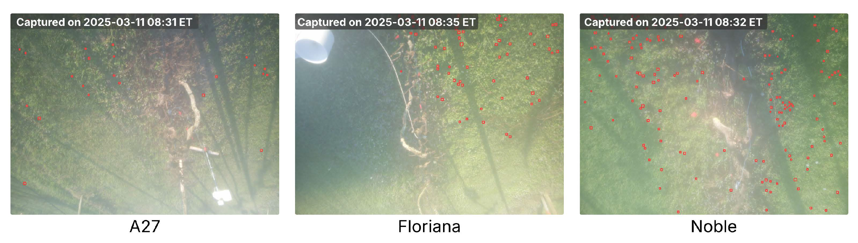
Figure 10.
Example of under-detected images processed by CC-trained Model 8. Detected buds are highlighted with red bounding boxes, and the non-detected buds are highlighted with orange bounding boxes.
Figure 10.
Example of under-detected images processed by CC-trained Model 8. Detected buds are highlighted with red bounding boxes, and the non-detected buds are highlighted with orange bounding boxes.
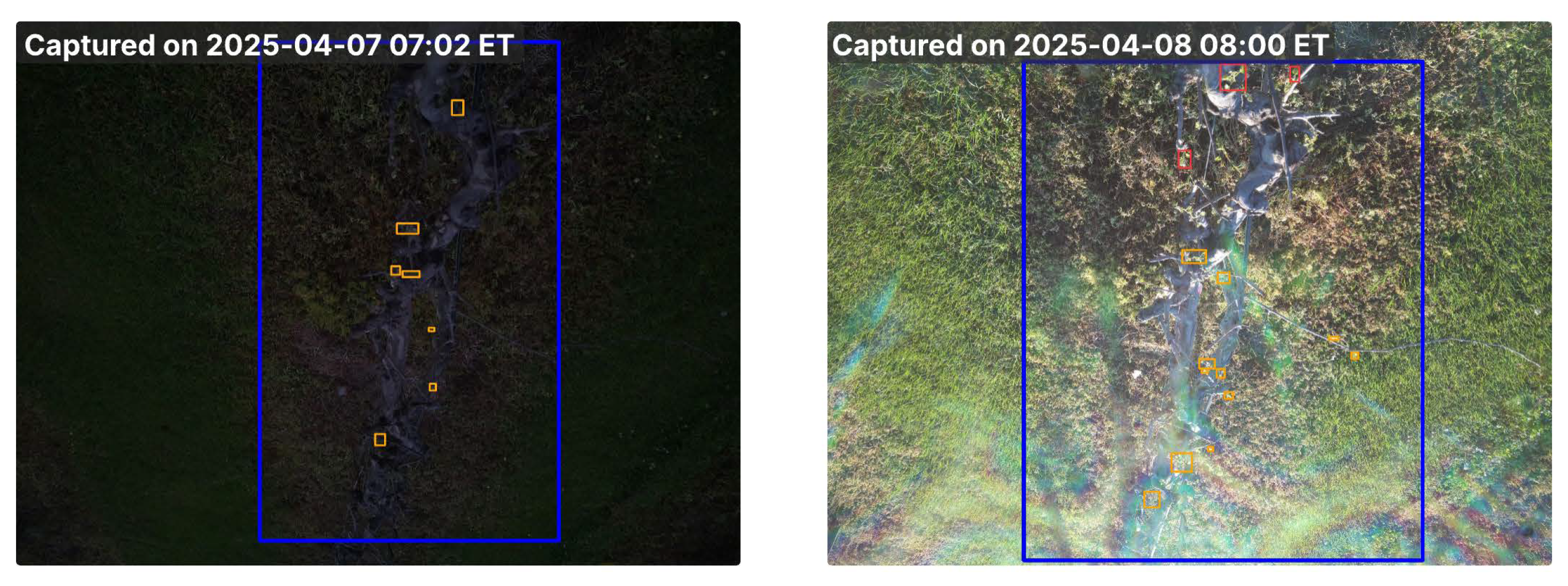
Figure 11.
Example dashboard view (NP6) showing raw counts at 30-minute intervals (Mar-Apr 2025). Results were produced by RG-trained Model 7. Available at https://phrec-irrigation.com/#/f/124/sensors/410.
Figure 11.
Example dashboard view (NP6) showing raw counts at 30-minute intervals (Mar-Apr 2025). Results were produced by RG-trained Model 7. Available at https://phrec-irrigation.com/#/f/124/sensors/410.
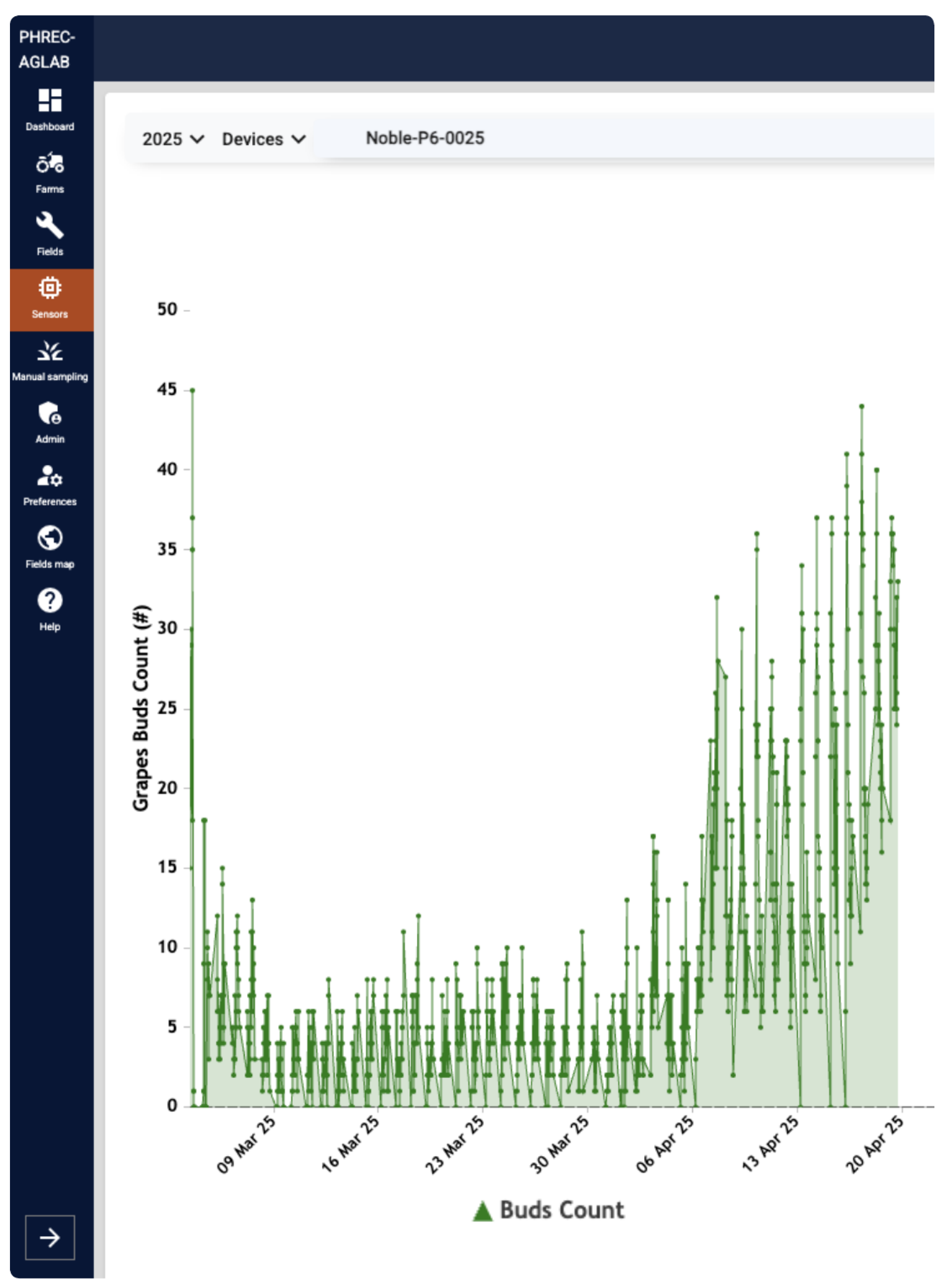

Table 1.
BudCAM node information including cultivar, harvest date, and bud break start and end dates.
Table 1.
BudCAM node information including cultivar, harvest date, and bud break start and end dates.
| Vine ID | Cultivar | Harvest Date | Start Date | End Date |
|---|---|---|---|---|
| FP2 | Floriana | 8/15/2024 | 3/24/2024 | 4/15/2024 |
| FP4 | Floriana | 8/15/2024 | 3/25/2024 | 4/8/2024 |
| FP6 | Floriana | 8/15/2024 | 3/26/2024 | 4/9/2024 |
| NP2 | Noble | 8/15/2024 | 3/26/2024 | 4/9/2024 |
| NP4 | Noble | 8/15/2024 | 3/26/2024 | 4/13/2024 |
| NP6 | Noble | 8/15/2024 | 3/24/2024 | 4/11/2024 |
| A27P15 | A27 | 8/20/2024 | 4/2/2024 | 4/20/2024 |
| A27P16 | A27 | 8/20/2024 | 3/30/2024 | 4/15/2024 |
| A27P17 | A27 | 8/20/2024 | 4/1/2024 | 4/20/2024 |
Table 2.
Distribution of raw images per vine from three Muscadine grape cultivars used for training, validation, and test in model development.
Table 2.
Distribution of raw images per vine from three Muscadine grape cultivars used for training, validation, and test in model development.
| Vine ID | Cultivar | Training | Validation | Test | Total |
|---|---|---|---|---|---|
| FP2 | Floriana | 168 | 52 | 43 | 263 |
| FP4 | Floriana | 133 | 24 | 30 | 187 |
| FP6 | Floriana | 233 | 51 | 47 | 331 |
| NP2 | Noble | 177 | 33 | 42 | 252 |
| NP4 | Noble | 299 | 80 | 65 | 444 |
| NP6 | Noble | 95 | 19 | 17 | 131 |
| A27P15 | A27 | 321 | 61 | 74 | 456 |
| A27P16 | A27 | 91 | 9 | 10 | 110 |
| A27P17 | A27 | 343 | 69 | 70 | 482 |
| – | Floriana total | 534 | 127 | 120 | 781 |
| – | Noble total | 571 | 132 | 124 | 827 |
| – | A27 total | 755 | 139 | 154 | 1048 |
Table 3.
Summary of the RG and CC datasets, including processing strategies, pipeline usage, and the number of samples in each subset after filtering.
Table 3.
Summary of the RG and CC datasets, including processing strategies, pipeline usage, and the number of samples in each subset after filtering.
| Dataset | Processing Strategy | Pipeline Usage | Training | Validation | Test | Total |
|---|---|---|---|---|---|---|
| RG | Raw image tiled into grid (776×864 px per tile) | Single-stage detector | 15,872 | 3387 | 3308 | 22,567 |
| CC | Cordon cropped and tiled into patches | Two-stage pipeline | 19,666 | 4147 | 4119 | 27,956 |
Table 4.
Parameter setting for two data augmentation configurations.
| Config. | Rotation | Translate | Scale | Shear | Perspective | Flip |
|---|---|---|---|---|---|---|
| Config. 1 | 45° | 40% | 30% | 10% | 0 | Yes |
| Config. 2 | 10° | 10% | 0 | 5% | 0.001 | Yes |
1 Configuration
Table 5.
Overview of the eight training configurations with variations in model size, fine-tuning, and data augmentation strategies.
Table 5.
Overview of the eight training configurations with variations in model size, fine-tuning, and data augmentation strategies.
| Model ID | Model Size | Fine-Tuned | Data Augmentation |
|---|---|---|---|
| Model 1 | Medium | No | None |
| Model 2 | Medium | Yes | None |
| Model 3 | Large | No | None |
| Model 4 | Large | Yes | None |
| Model 5 | Medium | No | Config 1 |
| Model 6 | Medium | Yes | Config 1 |
| Model 7 | Medium | No | Config 2 |
| Model 8 | Medium | Yes | Config 2 |
Table 6.
Performance and final training epochs for all model configurations.
| Model ID | Final Training Epoch | Test mAP@0.5 (%) |
|---|---|---|
| Trained on Raw Grid (RG) Dataset | ||
| Model 1 | 70 ± 25 | 75.9 ± 2.4 |
| Model 2 | 79 ± 34 | 80.3 ± 1.1 |
| Model 3 | 77 ± 25 | 76.0 ± 1.5 |
| Model 4 | 69 ± 24 | 78.5 ± 1.6 |
| Model 5 | 315 ± 69 | 85.1 ± 0.4 |
| Model 6 | 229 ± 30 | 85.3 ± 0.2 |
| Model 7 | 441 ± 70 | 86.0 ± 0.1 |
| Model 8 | 238 ± 43 | 85.7 ± 0.1 |
| Trained on Cordon-Cropped (CC) Dataset | ||
| Model 1 | 77 ± 4 | 79.1 ± 0.3 |
| Model 2 | 72 ± 10 | 78.3 ± 0.3 |
| Model 3 | 76 ± 4 | 79.2 ± 0.1 |
| Model 4 | 71 ± 9 | 78.7 ± 0.2 |
| Model 5 | 512 ± 60 | 84.4 ± 0.1 |
| Model 6 | 297 ± 103 | 84.4 ± 0.4 |
| Model 7 | 435 ± 27 | 84.7 ± 0.1 |
| Model 8 | 278 ± 45 | 85.0 ± 0.1 |
All numerical values are reported as mean ± standard deviation over five runs. Bold value indicates the best-performing model in each dataset group.
Table 7.
Performance comparison of the top models under different inference strategies.
| Model | Baseline | Resized-CC | Sliced-CC |
|---|---|---|---|
| Model 7 (RG) | 86.0 ± 0.1 | 58.2 ± 1.3 | 74.8 ± 0.7 |
| Model 8 (CC) | 85.0 ± 0.1 | 52.6 ± 1.0 | 80.0 ± 0.2 |
All scores are mAP@0.5 (%) reported as mean ± standard deviation. Bold values indicate the best performance for each model. Performance on the model’s corresponding standard test set (RG or CC), which uses a tiling approach. Sliding-window inference with a slice-overlap ratio of 0.2.
Table 8.
Comparison of mAP@0.5 scores (%, mean ± SD) under three slice-overlap ratios for the top-performing models.
Table 8.
Comparison of mAP@0.5 scores (%, mean ± SD) under three slice-overlap ratios for the top-performing models.
| Model | Slice-overlap ratio | ||
|---|---|---|---|
| 0.2 | 0.5 | 0.75 | |
| Model 7 (RG) | 74.8 ± 0.7 | 72.0 ± 0.7 | 66.3 ± 0.6 |
| Model 8 (CC) | 80.0 ± 0.2 | 76.4 ± 0.4 | 69.2 ± 0.5 |
All scores are mAP@0.5 (%) reported as mean ± standard deviation. Bold values indicate the best performance for each model.
Table 9.
Comparison of methods related to bud/seedling detection or segmentation.
| Method | Model | Dataset | View / Camera Angle | Platform | Performance |
|---|---|---|---|---|---|
| BudCAM (this work) | YOLOv11-m (RG, M7) | 2,656 images; px | Nadir, 1–3 m above vines | Raspberry Pi 5 | 86.0 (mAP@0.5) |
| YOLOv11-m (CC, M8) | 85.0 (mAP@0.5) | ||||
| Grimm et al. [7] | UNet-style (VGG16 encoder) | 542 images; up to px | Side view, within ∼2 m | – | 79.7 (F1) |
| Rudolph et al. [8] | FCN | 108 images; px | Side view, within ∼1 m | – | 75.2 (F1) |
| Marset et al. [9] | FCN–MobileNet | 698 images; px | – | – | 88.6 (F1) |
| Xia et al. [6] | ResNeSt50 | 31,158 images; up to px | 0.4–0.8 m | – | 92.4 (F1) |
| Li et al. [4] | YOLOv4 | 7,723 images; px | – | – | 85.2 (mAP@0.5) |
| Gui et al. [5] | YOLOv5-l | 1,000 images; px | – | – | 92.7 (mAP@0.5) |
| Chen et al. [17] | YOLOv8-n | 4,058 images; px | UAV top view, ∼3 m AGL | – | 99.4 (mAP@0.5) |
| Pawikhum et al. [20] | YOLOv8-n | 1,500 images | Multi-angles, ∼0.5 m | Edge (embedded) | 59.0 (mAP@0.5) |
All scores are as reported by the respective papers; tasks and metrics differ (detection vs. segmentation; F1 vs. mAP) and are not strictly comparable. RG-trained Model 7. CC-trained Model 8.
Disclaimer/Publisher’s Note: The statements, opinions and data contained in all publications are solely those of the individual author(s) and contributor(s) and not of MDPI and/or the editor(s). MDPI and/or the editor(s) disclaim responsibility for any injury to people or property resulting from any ideas, methods, instructions or products referred to in the content. |
© 2025 by the authors. Licensee MDPI, Basel, Switzerland. This article is an open access article distributed under the terms and conditions of the Creative Commons Attribution (CC BY) license (http://creativecommons.org/licenses/by/4.0/).
Copyright: This open access article is published under a Creative Commons CC BY 4.0 license, which permit the free download, distribution, and reuse, provided that the author and preprint are cited in any reuse.


