Development of a Low-Cost, Open-Source Quartz Crystal Microbalance with Dissipation Monitoring for Potential Biomedical Applications

Gabriel Guillermo Muñoz; Martín Javier Millicovsky; Albano Peñalva; Juan Ignacio Cerrudo; Juan Manuel Reta; Martín Angel Zalazar

doi:10.20944/preprints202509.2523.v1

Submitted:

29 September 2025

Posted:

30 September 2025

You are already at the latest version

Abstract

Quartz Crystal Microbalance with Dissipation monitoring (QCM-D) systems are widely used for the real-time analysis of mass changes and viscoelastic properties in biological samples, enabling applications such as biomolecular interaction studies, biosensing, and fluid characterization. However, their accessibility has been limited by high acquisition costs. To address this limitation, the development of a low-cost, open-source QCM-D system tailored for biomedical applications has been carried out. A 10 MHz quartz crystal with a sensor module and a control and acquisition unit were integrated. The full system was built at a total cost below USD 500. Performance validation showed a temperature stability of ±0.13°C, a frequency stability of ±2 Hz in air, and a limit of detection of 0.46% polyethylene glycol (PEG) in batch mode. These results demonstrate that key sensing capabilities can be achieved at a fraction of the cost, making it a viable alternative for certain biomedical applications. Its open-source nature allows full customization and future upgrades, offering a flexible alternative for laboratories seeking affordable yet reliable tools for biophysical analysis.

Keywords:

quartz crystal microbalance

;

open-source hardware

;

real-time monitoring

;

viscoelastic properties

;

biomedical applications

Subject:

Engineering - Bioengineering

1. Introduction

Sensors are regarded as essential tools in modern science and technology, enabling the detection and quantification of physical, chemical, and biological phenomena across a broad range of applications [1]. Among these, piezoelectric sensors are distinguished by their reliance on the piezoelectric effect, through which certain materials are induced to generate an electrical charge in response to mechanical stress or deformation [2]. This effect has been utilized to detect changes in pressure, force, or mass, with the resulting electrical signals being readily measurable and interpretable [3]. In laboratory environments dedicated to biomolecular analysis, diagnostic testing, and disease research, piezoelectric sensors have been employed to provide real-time, non-destructive, and highly sensitive measurements that contribute to experimental insights and support clinical decision-making [4].

The Quartz Crystal Microbalance (QCM) has been widely adopted as a piezoelectric technique for the investigation of surface interactions at the nanoscale [5,6]. In this method, changes in the resonant frequency (f_r) of a quartz crystal sensor are monitored as mass is deposited on or removed from its surface [7]. An advanced variant, known as Quartz Crystal Microbalance with Dissipation Monitoring (QCM-D), has been designed to simultaneously measure both the frequency shift and the dissipation factor (D), the latter representing energy loss due to oscillation damping. This dual-mode sensing capability has enabled the characterization of mass, viscoelastic properties, and the dynamic behavior of the interacting materials [8].

QCM-D systems have been increasingly employed in biomedical applications such as biosensing, drug delivery monitoring, and biomolecular interaction studies [9,10,11,12]. Nevertheless, the adoption of these systems has often been hindered by high operational costs, particularly in resource-limited contexts [13]. While commercial platforms from manufacturers such as AWSensores, Biolin Scientific and Gamry Instruments have been designed to offer robust and high-performance solutions [14,15], their elevated costs have restricted their availability in many research environments. Alternatively, various experimental QCM setups have been developed within academic settings, often demonstrating promising performance but lacking the robustness, ease of use, or system integration necessary for broader implementation [16,17]. Similarly, other piezoelectric sensors, such as Surface Acoustic Wave (SAW) devices, have been investigated through low-cost experimental platforms, further highlighting the versatility of acoustic wave-based sensing technologies, although generally not reaching the same level of performance demonstrated by QCM-D systems [18,19].

To overcome these challenges, this work presents an improved QCM-D system based on a previous prototype version developed by the authors [20]. Significant changes were done with the aim of enhancing thermal stability, sensitivity, and cost-efficiency. The developed system has been optimized to be more robust and adaptable to a wider range of laboratory applications. In addition to f_r, the system also enables D measurements, broadening its applicability to viscoelastic characterization. The following sections present the design, fabrication, and experimental validation of this improved QCM-D system, which is intended to contribute to the advancement of accessible and reliable piezoelectric platforms for biomedical research and diagnostics.

2. Design

The QCM-D system (Figure 1) consists of a quartz crystal (Figure 1A) placed in a sensor module (Figure 1B), which connects via an SMA connector (Amphenol) and gold-plated pogo pins (Preci-Dip) to a control and acquisition unit (Figure 1C).

An AT-cut piezoelectric quartz crystal disc with a fundamental frequency of 10 MHz, coated with gold electrodes (Novaetech SRL), was used; it has a thickness of 160 µm and a nominal sensitivity of 4.42 × 10⁻⁹ g·Hz⁻¹·cm⁻², with front and back electrode diameters of 11.5 mm and 6 mm, respectively.

The sensor module was designed using Fusion 360 (Autodesk Inc.) and fabricated through masked stereolithography 3D printing (Creality LD-006) with photosensitive resin (Monoprice). The module dimensions are 44 mm in width, 40 mm in length, and 15 mm in height, with a weight of 21.5 g.

The control and acquisition unit integrates a temperature control system based on a TEC1-12706 Peltier cell (MikroElektronika) and a frequency measurement instrument, the NanoVNA-H (from the open-source NanoVNA series). A protective cover (gray box in Figure 1C) is included to minimize external perturbations and to improve thermal control.

2.1. Sensor Module

The design prioritizes low maintenance, allowing quick and easy positioning of the crystal. The top (Figure 2.M1) is secured to the base (Figure 2.M2) using screws that fasten into pre-installed inserts (E-Z Lok) (Figure 2.M3), ensuring a firm and durable assembly. A silicone O-ring (Seals R Us) (Figure 2.M4) in contact with both faces of the crystal maintains stable pressure and prevents liquid leakage. The sensor module includes a custom-designed circuit board (PCB) (Figure 2.M5) developed using the open-source software KiCad, specifically for crystal measurements with the NanoVNA-H. Electrical connection was made using gold-plated pogo pins (Figure 2.M6) and a low-noise SMA connector (Figure 2.M7) to ensure reliable signal transmission. Additionally, a ventilation system was incorporated to improve temperature distribution.

2.2. Control and Acquisition Unit

The Peltier cell (Figure 3.CA1) supplied with 12 V and 6 A, was selected as the thermoelectric device. An aluminum heat sink, together with thermal grease and a fan (Intel) (Figure 3.CA2), favor the temperature difference between both Peltier faces. Thermal control has a 18°C-30°C nominal working range, and bidirectional heating and cooling. A Raspberry Pi Pico microcontroller (Raspberry Pi Foundation) (Figure 3.CA3) was selected for a proportional-integral-derivative (PID) control. Temperature acquisition was measured using an NTC 3950 thermistor (Eaton) (Figure 3.CA4), which offers fast response time and high precision. The firmware to control the temperature was developed in C language specifically to be executed on a Raspberry Pi Pico. The Peltier cell current was driven through a Pulse Width Modulation (PWM) signal generated by the Raspberry Pi. A dual-channel H-bridge motor driver, VNH2SP30 (Reland Sun) (Figure 3.CA5), rated at 30 A, was used for this purpose. A 12 V / 10 A switching power supply (MeanWell) (Figure 3.CA6) was selected to supply power to the motor driver, cooling fan, Peltier cell, and the Raspberry Pi Pico.

The frequency measurement instrument integrated into the QCM housing is the NanoVNA-H (Figure 3.CA7), a compact vector network analyzer capable of measuring S-parameters (S11, S21) with a frequency range from 10 kHz to 1.5 GHz. It provides up to 70 dB of dynamic range at low frequencies (50 kHz – 300 MHz), with 101 scanning points per sweep, ensuring suitable resolution for frequency tracking. The device features an USB-C interface for data transfer and charging, and an internal 650 mAh lithium battery.

2.3. NanoVNA Software

The open-source software of the NanoVNA-type H device, originally developed in Python 3.9, was customized to address the specific requirements of biosensing applications. Non-essential tools were removed, the user interface was redesigned, and algorithms were implemented to enable real-time analysis of f_r, D, and temperature. From this curve, the f_r is identified as the point where conductance reaches its maximum value, while D is calculated based on the bandwidth of the signal [21]. Repeated sweeps are performed over a defined period to monitor the behavior of the sensor over time. Temperature is recorded during each acquisition, allowing for the evaluation of thermal effects on the measurements. The software also includes a calibration assistant to streamline the calibration process. Harmonics can be measured, though not simultaneously, up to the 9th harmonic, providing additional information about the properties of the sample.

The program can be executed in Python environments such as PyCharm or Visual Studio, or compiled into a standalone executable. In both cases, a line in the SweepWorker file must be edited to specify the directory where Touchstone files from the continuous sweep will be saved. During multi-segment sweeps, real-time data updates are displayed along with markers highlighting key values. Sweep data can be exported in .xlsx format, focused on the f_r, D, and temperature parameters. Figure 4 presents the customized software in operation, showing the configuration section and the real-time visualization of the recorded data.

3. Build Instructions

3.1. Materials and Tools

Basic tools such as a soldering iron, leaded solder wire, wire cutters, screwdrivers, tweezers, and multimeters are required for building the device

Table 1. Design files summary.

Designator	Filename	File Type¹	Localization of file
D1	Top_sensor_module	3D Printing	Supplementary Materials
D2	Base_sensor_module	3D Printing	Supplementary Materials
D3	Protective_cover	3D Printing	Supplementary Materials
D4	Back_legs_housing	3D Printing	Supplementary Materials
D5	Front_legs_housing	3D Printing	Supplementary Materials
D6	Internal_base_housing	3D Printing	Supplementary Materials
D7	VNA_port_cover	3D Printing	Supplementary Materials
D8	Back_fan_trim	3D Printing	Supplementary Materials
D9	Fan_bracket	3D Printing	Supplementary Materials
D10	Top_holder	3D Printing	Supplementary Materials
D11	Vent_cover	3D Printing	Supplementary Materials
D12	PCB_from_Kicad	PCB Design	Supplementary Materials
D13	Raspberry_Pi_firmware	Software	Supplementary Materials
D14	Device_Software	Software	Supplementary Materials

¹ Open Source License: Creative Commons Attribution 4.0 International.

Table 2. Bill of materials.

Designator	Component	Number	Cost per Unit - USD	Total cost – USD	Source of Material
M1	^Base_sensor_module	1	37.58	37.58	AMAZON
M2	^Top_sensor_module	1	37.58	37.58	AMAZON
M3	Insert	2	0.09	0.18	AMAZON
M4	Pogo-pin	2	1.06	2.12	DIGIKEY
M5	O-ring	2	2.72	5.44	eBAY
M6	PCB board	1	7.29	7.29	AMAZON
M7	SMA Connector	1	10.66	10.66	MOUSER
E1	Housing	1	50.00	50.00	PRODUCTOS TERMOFORMADOS S.R.L
E2	*Internal base housing	1	24.69	24.69	AMAZON
E3	*Top holder	1	24.69	24.69	AMAZON
E4	*Fan bracket	1	24.69	24.69	AMAZON
E5	*Protective_cover	1	24.69	24.69	AMAZON
E6	*VNA port cover	1	24.69	24.69	AMAZON
E7	*Back fan trim	1	24.69	24.69	AMAZON
E8	*Vent cover	2	24.69	24.69	AMAZON
E9	*Legs	4	24.69	24.69	AMAZON
CA1	TEC1-12706Peltier cell	1	10.80	10.80	DIGIKEY
CA2	Fan and Heatsink 12 V 0.6 A	1	20.00	20.00	eBAY
CA3	Raspberry Pi Pico	1	18.65	18.65	AMAZON
CA4	NTC 3950 analog sensor	1	0.55	0.55	DIGIKEY
CA5	VNH2SP30 30A 2-channel stepper motor driver	1	42.00	42.00	AMAZON
CA6	Power supply 12V/10A	1	20.57	20.57	AMAZON
CA7	Nano Vector Network Analyzer	1	40.85	40.85	eBAY
CA8	12V, 80mm fan	2	5.05	10.10	DIGIKEY
CA9	Resistor 100Kohm	1	0.03	0.03	DIGIKEY
CA10	Electrolity Capacitor	1	0.03	0.03	AMAZON
PC1	Power Cable	1	3.0	3.0	DIGIKEY
PC2	Power connector	1	2.0	2.0	DIGIKEY
PC3	2-Channel Relay Module for Arduino 12V	1	4.0	4.0	eBAY
PC4	Switch	1	1.0	1.0	DIGIKEY
PC5	Hub	1	6.88	6.88	AMAZON
PC6	15 cm USB-A to Micro USB Cable	2	3.03	6.06	eBAY
PC7	15 cm USB-A to USB-C Cable	2	2.00	4.00	eBAY
PC8	USB Type-A Male to Type-B Male Cable	1	1.00	2.00	eBAY
PC9	Crystal openQCM 10MHz	10	28.40	284.00	open QCM

*3D printed parts with polylactic acid (PLA), a single 1.75 mm 1 kg PLA filament was used, its cost is $24.69. ^3D printed parts with resin.

3.2. Sensor Module Construction

Fabricate the PCB (M5).
Solder the SMA connector (M7) and pogo-pins (M6) onto the assembled PCB.
Print the pieces (M1, M2) with a 3D printer.
Attach the soldered PCB (step 2) to the sensor module base (M1) using glue.
Insert O-Ring (M4) into the base and the upper part of the sensor module. Press the O-rings.
Insert two pogo pins (M6) where the lower O-ring sits.
Place two inserts (M3) in M2.
Perform a leak test. Before adding the liquid, insert two strips of paper between module parts and wait one hour to identify if papers are wet.

3.3. Housing and Accessories

Print the 3D accessories (Figure 5).
Mark and drill holes in the housing (E1) for the air outlet, the Peltier module, and the power and signal connectors.
Mount the 3D-printed accessories inside the E1.
Attach the components into the pre-cut holes.
Secure all elements with screws or adhesive as needed.
Ensure proper airflow and cable routing inside the housing.

3.4. Power Supply and Communication

Connect a 12 V / 10 A power supply (CA6) via a power connector (PC2) to a power cable (PC1) that plugs into the mains.
Install a switch (PC4) in series with the live line to allow manual control of power delivery.
The power supply will directly power all cooling fans (CA2, CA8) and the VNH2SP30 30 A dual-channel motor driver (CA5).
Use a commercial USB hub (PC5) to establish serial communication between the NanoVNA (CA7), Raspberry Pi Pico (CA3), and the USB cable (PC8) connected to the PC.
Integrate two relays (PC3) that act as switches, allowing the Raspberry Pi Pico and NanoVNA to power on only when the power supply is active

3.5. Temperature Control

To load the firmware onto the Raspberry Pi Pico, connect the Pico to the USB port while holding down the BOOTSEL button. It will mount as a storage device named RPI-RP2. Download the firmware from GitHub, then drag and drop the .uf2 file onto the RPI-RP2 drive.
Connect an electrolytic capacitor (CA10) between pins 36 and 35 of the Raspberry Pi Pico to filter noise.
Build a resistive voltage divider with NTC 3950. Connect the NTC 3950 between 3.3 V (pin 36) and the middle node (pin 34). Connect a fixed 100 kΩ resistor from the middle node to GND (pin 33).
Connect VNH2SP30 motor driver (CA5) to the Raspberry Pi Pico (CA3) making the following connections:
- VNH2SP30 GND to Raspberry Pi Pico GND (pin 39)
- VNH2SP30 +5 V to Raspberry Pi Pico 5 V (pin 40)
- VNH2SP30 EN1 to Raspberry Pi Pico (pin 17)
- VNH2SP30 B1 to Raspberry Pi Pico (pin 14)
- VNH2SP30 A1 to Raspberry Pi Pico (pin 15)
- VNH2SP30 PWM to Raspberry Pi Pico (pin 16)
Connect the VNH2SP30 motor driver (CA5) to the power supply (CA6) and then connect the Peltier cell (CA1) to the output terminals A1 and B1 of the motor driver.

4. Operating Instructions

4.1. Sensor Module Assembly and Usage

The sensor module is composed of two main parts: the top and the base. The base contains pogo pins, which establish the electrical connection with the QCM crystal. The assembly and usage procedure was performed as follows:

The screws were loosened using an Allen wrench.
The base was separated from the top, and the top was placed with the inner side facing upward.
The quartz crystal was positioned onto the O-ring inside the top.
The base was repositioned onto the top.
It was verified that the electrodes on the back of the crystal were in proper contact with the pogo pins on the base.
The screws were tightened with the Allen wrench to securely close the sensor module.

The liquid sample was then deposited directly onto the crystal surface using a micropipette (Figure 6), and the sealed measurement chamber was placed over the sensor module to ensure stable conditions and optimal contact.

4.2. Crystal Cleaning

The cleaning strategy can be adapted according to the characteristics of the sample (see Figure 7). Below, a specific cleaning method for the non-functionalized crystal is described.

4.3. Custom Software

Once the system setup is complete and the NanoVNA is connected to the PC, the device is turned on and the software is launched. The program automatically detects the instrument and its communication port. A continuous sweep is initiated by clicking the "Connect" button, which performs a basic sweep. During these initial sweeps, the sweep parameters are adjusted to achieve the desired resolution and timing. In the sweep configuration panel, the "Find Resonance" option is selected to determine the working frequency and conduct a refined sweep. Subsequently, the "Continuous Sweep" function is activated and the number of sweeps to be performed is specified according to the required acquisition time. The resulting Touchstone files are saved in the previously selected directory. After the acquisition is complete, the data is exported in .xlsx format by selecting "Save Data."

5. Validation

5.1. Temperature Performance

The system was evaluated across a temperature range of 18°C to 30 °C, with 4 °C increments. At each step, the system was held at the target temperature for 30 minutes to assess the time required to reach and maintain thermal stability. Figure 8 shows the temperature profile over time during the entire thermal cycling protocol.

The mean and standard deviation (SD) of the temperature at each setpoint were calculated, as shown in Table 3. The average SD across all stable intervals was ±0.13 °C.

The temperature for extracting technical features was determined by evaluating the stability of f_r and D at the third harmonic, which provides higher sensitivity to variations in mass and viscoelastic properties than the fundamental frequency [22]. Measurements were taken after one hour of thermal equilibration. The condition with the lowest variability in both parameters—quantified through SD—was considered the most stable.

A temperature of 26 °C was selected, as it exhibited the lowest SD in both f_r and D. At this temperature, the measurements in air showed a frequency stability with a SD of ±2 Hz and a dissipation stability within ±0.0001 × 10⁻⁶ over one hour. In measurements with distilled water, the SD was ±19 Hz for f_r and ±0.0021 × 10⁻⁶ for D. Analysis of the initial data indicates that a minimum stabilization time of approximately 15 minutes is sufficient to reach acceptable measurement of f_r and D.

Complete results for all temperature levels are provided in the Supplementary Material.

5.2. Analytical Validation: Repeatability, Sensitivity, and Limit of Detection

To assess repeatability, sensitivity (S), and limit of detection (LOD), measurements of water and different concentrations of PEG (2%, 5%, and 10%) were taken on three consecutive days, under controlled temperature conditions (26 °C) (see Figure 9).

As shown in Figure 9, measurements performed over three consecutive days exhibited consistent responses across all PEG concentrations. The standard deviations remained below 365 Hz for frequency and 0.67 × 10⁻⁶ for dissipation, confirming good interday repeatability.

Sensitivity was calculated as the slope of the linear regression of the steady-state frequency and dissipation shifts relative to distilled water, across increasing PEG concentrations (see Figure 10). This approach allows quantifying the response of the sensor to increasing viscoelastic loading. The calculated frequency sensitivity was -284.82 Hz per 1% PEG, while the dissipation sensitivity was 0.294 × 10⁻⁶ per 1% PEG.

With a sensitivity of -284.82 Hz per 1% PEG and a baseline SD of 40 Hz, the LOD was estimated using the formula LOD = 3.3×SD/S [23], resulting in approximately 0.46% PEG. This means that the sensor can detect PEG concentrations starting from around 0.46%, indicating good sensitivity for dilute solutions. This estimation follows IUPAC guidelines, which calculate the LOD based on the signal-to-noise ratio of the baseline and the sensitivity of the sensor [24].

6. Conclusions

In this study, the design, construction, and experimental validation of a low-cost, open-source QCM-D system for biomedical applications were carried out. The platform was developed using readily available components, including a NanoVNA-H for frequency acquisition and a Raspberry Pi Pico for temperature control, all integrated into housing with active thermal regulation. Custom software was implemented for real-time monitoring of frequency, dissipation, and temperature.

The system demonstrated reliable performance in key areas: a temperature stability of ±0.13 °C, a frequency resolution of ±2 Hz in air, and a dissipation stability of ±0.0001 × 10⁻⁶ under steady-state conditions. Repeatability tests with PEG solutions (2%, 5%, 10%) over three consecutive days showed SD below 365 Hz in batch mode, confirming robust interday consistency. Sensitivity analyses yielded −284.82 Hz/%PEG and 0.294 × 10⁻⁶/%PEG. Based on baseline variability, the LOD was estimated at 0.46%.

Compared to commercial systems, the developed prototype is noted for its accessibility. While instruments such as the QSense Omni (Biolin Scientific) and X4 Advanced Multichannel QCM-D system (AWSensors) offer a wide array of advanced features, including nanogram-level sensitivity, sub-Hz frequency stability, multi-overtone capabilities, and automated sample handling, these benefits come at a cost exceeding USD 30,000. In contrast, the presented system achieves sensing functionality for under USD 500.

Several limitations should be acknowledged: loss of information due to the use of a single harmonic; temperature regulation, while effective, does not match the precision of commercial temperature-control modules; the absence of an integrated fluidic handling system limits automation; and the current sensor module design, optimized for batch operation, lacks flow-mode capabilities and would benefit from more durable materials.

Future developments will be directed toward refining thermal control, enabling the simultaneous measurement of harmonics, enhancing time resolution, and integrating fluidic automation. The system is thus positioned as a viable tool for early-stage research and the democratization of QCM-D technology in biomedical contexts.

Supplementary Materials

The following supporting information can be downloaded at the website of this paper posted on Preprints.org.

Name	Type	Description
3D Models and Hardware	Zip	STL files for system fabrication and PCB design file
Figures and Results	Zip	Article figures and complete validation results
Software and Firmware	Zip	Device software (developed in Python) and Raspberry Pi firmware for temperature control

Author Contributions

Conceptualization, Muñoz G., Peñalva A., Cerrudo J., and Zalazar M.; methodology, Muñoz G., Millicovsky M., and Zalazar M.; software, Muñoz G. and Millicovsky M.; validation, Muñoz G. and Zalazar M.; formal analysis, Muñoz, G.; investigation, Muñoz, G and Zalazar M.; resources, Reta J., Cerrudo J., Peñalva A., and Zalazar M.; data curation, Muñoz G.; writing—original draft preparation, Muñoz G. and Zalazar M.; writing—review and editing, Muñoz G., Peñalva, A., Cerrudo J., Millicovsky M. and Zalazar M.; visualization, Muñoz G., Millicovsky M. and Zalazar M.; supervision, Zalazar M.; project administration, Reta J. and Zalazar M.; funding acquisition, Reta J. and Zalazar M. All authors have read and agreed to the published version of the manuscript.

Funding

This research was funded by AGENCIA NACIONAL DE PROMOCIÓN CIENTÍFICA Y TECNOLÓGICA, grant number PICT StartUp 2022-00014 Desarrollo de biosensor basado en tecnología de microbalanza de cristal de cuarzo para el diagnóstico de síndrome de ojo seco, Argentina.

Institutional Review Board Statement

Not applicable.

Informed Consent Statement

Not applicable.

Data Availability Statement

The data are available in the Supplementary Materials.

Acknowledgments

We would like to express our gratitude to the Laboratorio de Prototipado e Impresión 3D at the Facultad de Ingeniería, Universidad Nacional de Entre Ríos, Argentina, for providing the facilities for the development and evaluation of our device.

Conflicts of Interest

The authors declare no conflicts of interest.

Abbreviations

The following abbreviations are used in this manuscript:

CA	Control and Acquisition Unit
D	Dissipation
f_r	Resonance Frequency
LOD	Limit of Detection
M	Sensor Module
NTC	Negative Temperature Coefficient
PCB	Printed Circuit Board
PEG	Polyethylene glycol
PID	Proportional-Integral-Derivative
PLA	Polylactic acid
QCM	Quartz Crystal Microbalance
S	Sensitivity
SAW	Surface Acoustic Wave
SD	Standard Deviation
SMA	SubMiniature version A
VNA	Vector Network Analyzer

References

Javaid, M.; Haleem, A.; Rab, S.; Singh, R. P.; Suman, R. Sensors for daily life: A review. Sens Int 2021, 2, 100121. [Google Scholar] [CrossRef]
Shaukat, H.; Ali, A.; Bibi, S.; Altabey, W.A.; Noori, M.; Kouritem, S.A. A Review of the Recent Advances in Piezoelectric Materials, Energy Harvester Structures, and Their Applications in Analytical Chemistry. Appl. Sci 2023, 13, 1300. [Google Scholar] [CrossRef]
Jiao, P.; Egbe, K. J.; Xie, Y.; Matin Nazar, A.; Alavi, A.H. Piezoelectric Sensing Techniques in Structural Health Monitoring: A State-of-the-Art Review. Sensors 2020, 20, 3730. [Google Scholar] [CrossRef]
Kaushal, J.B.; Raut, P.; Kumar, S. Organic Electronics in Biosensing: A Promising Frontier for Medical and Environmental Applications. Biosensors 2023, 13, 976. [Google Scholar] [CrossRef]
Na Songkhla, S.; Nakamoto, T. Overview of quartz crystal microbalance behavior analysis and measurement. Chemosensors 2021, 9, 350. [Google Scholar] [CrossRef]
Alanazi, N. , Almutairi, M.; Alodhayb, A. A Review of Quartz Crystal Microbalance for Chemical and Biological Sensing Applications. Sens Imaging 2023, 24. [Google Scholar]
Huang, X.; Chen, Q.; Pan, W.; Yao, Y. Advances in the Mass Sensitivity Distribution of Quartz Crystal Microbalances: A Review. Sensors 2022, 22, 5112. [Google Scholar] [CrossRef] [PubMed]
Easley, A.D.; Ma, T.; Eneh, C.I.; Yun, J.; Thakur, R.M.; Lutkenhaus, J.L. A practical guide to quartz crystal microbalance with dissipation monitoring of thin polymer films. J Polym Sci 2021, 60, 1090–1107. [Google Scholar] [CrossRef]
Palleschi, S.; Silvestroni, L.; Rossi, B.; Dinarelli, S.; Magi, M.; Giacomelli, A.; Bettucci, A. Simple and sensitive method for in vitro monitoring of red blood cell viscoelasticity by Quartz Crystal Microbalance with dissipation monitoring (QCM-D). Biosens Bioelectron X 2024, 21, 100554. [Google Scholar] [CrossRef]
Chen, Z.; Zhou, T.; Hu, J.; Duan, H. Quartz Crystal Microbalance with Dissipation Monitoring of Dynamic Viscoelastic Changes of Tobacco BY-2 Cells under Different Osmotic Conditions. Biosensors 2021, 11, 136. [Google Scholar] [CrossRef]
MuYilmaz-Aykut, D.; Yolacan, O.; Deligoz, H. A comparative QCM-D study for various drug sorption behaviors and chemical degradation of chitosan/PAA LbL multilayered films. J Polym Res 2023, 30(8), 307. [Google Scholar] [CrossRef]
Muñoz, G.G.; Millicovsky, M.J.; Cerrudo, J.I.; Peñalva, A.; Machtey, M.; Reta, J.M.; Torres, R.M.; Campana, D.M.; Zalazar, M.A. Exploring tear viscosity with quartz crystal microbalance technology. Rev Sci Instrum 2024, 75, 075107. [Google Scholar] [CrossRef] [PubMed]
Hampitak, P.; Jowitt, T. A.; Melendrez, D.; Fresquet, M.; Hamilton, P.; Iliut, M.; Nie, K.; Spencer, B.; Lennon, R.; Vijayaraghavan, A. A point-of-care immunosensor based on a quartz crystal microbalance with graphene biointerface for antibody assay. ACS Sensors 2020, 5, 3520–3532. [Google Scholar] [CrossRef] [PubMed]
Biolin Scientific. https://www.biolinscientific.com (accessed on 03 04 2025).
Gamry Intruments. https://www.gamry.com/ (accessed on 25 08 2025).
Adel, M.; Allam, A.; Sayour, A.E.; Ragai, H.F.; Umezu, S. , Fath El-Bab, A.M.R. Design and development of a portable low-cost QCM-based system for liquid biosensing. Biomed Microdevices 2024, 26, 11. [Google Scholar] [CrossRef]
Melendrez, D.; Hampitak, P.; Jowitt, T.; Iliut, M.; Vijayaraghavan, A. Development of an open-source thermally stabilized quartz crystal microbalance instrument for biomolecule-substrate binding assays on gold and graphene. Anal Chim Acta 2021, 1156, 338329. [Google Scholar] [CrossRef]
Millicovsky, M.; Schierloh, L.; Kler, P.; Muñoz, G.; Cerrudo, J.; Peñalva, A.; Reta, J.; Zalazar, M. Low-Cost Open-Source Biosensing System Prototype Based on a Love Wave Surface Acoustic Wave Resonator. Hardware 2025, 3, 9. [Google Scholar] [CrossRef]
Nair, M.P.; Teo, A.J.T.; Li, K.H.H. Acoustic Biosensors and Microfluidic Devices in the Decennium: Principles and Applications. Micromachines 2022, 13, 24. [Google Scholar] [CrossRef]
Muñoz, G.G.; Millicovsky, M.J.; Reta, J.M.; Cerrudo, J.I.; Peñalva, A.; Machtey, M.; Torres, R.M.; Zalazar, M.A. Quartz crystal Microbalance with dissipation monitoring for biomedical applications: Open source and low cost prototype with active temperature control. Hardware X 2023, 14, e00416. [Google Scholar] [CrossRef]
Carvajal Ahumada, L.A.; Sandoval Cruz A., F.; García Foz M., A.; Herrera Sandoval O., L. Useful piezoelectric sensor to detect false liquor in samples with different degrees of adulteration. J Sens 2018, 218, 6924094. [Google Scholar] [CrossRef]
Corradi, E.; Agostini, M.; Greco, G.; Massidda, D.; Santi, M.; Calderisi, M.; Signore, G.; Cecchini, M. An objective, principal-component-analysis (PCA) based, method which improves the quartz-crystal-microbalance (QCM) sensing performance. Sens Actuator Phys 2020, 315, 112323. [Google Scholar] [CrossRef]
Izsák, T.; Varga, M.; Kočí, M.; Szabó, O.; Dragounová, A.K.; Vanko, G.; Gál, M.; Korčeková, J.; Hornychová, M.; Poturnayová, A.; Kromka, A. Diamond-coated quartz crystal microbalance sensors: Challenges in high yield production and enhanced detection of ethanol and sars-cov-2 proteins. Mater Des 2024, 248, 113474. [Google Scholar] [CrossRef]
IUPAC Compendium of Chemical Terminology, 5th ed. International Union of Pure and Applied Chemistry; 2025. Online version 5.0.0, 2025. [CrossRef]

Figure 1. QCM system. The quartz crystal (A) is positioned within the sensor module (B), which is placed on the Peltier element, located in the housing containing the control and acquisition unit (C). Samples are deposited into the sensor module, after which a protective cover (gray box in C) is placed over it. Temperature control is then initiated prior to acquiring the corresponding measurements.

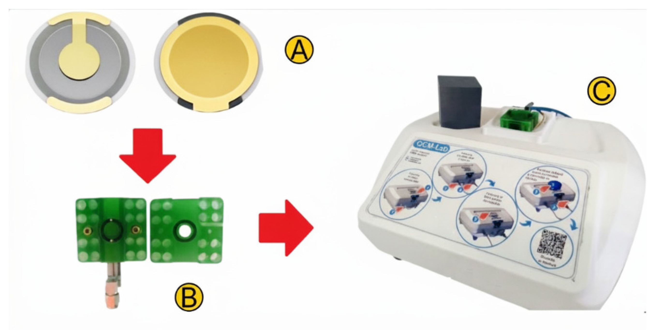
Figure 2. 3D-printed sensor module (M). M1) Top. M2) Base. M3) Inserts. M4) O-ring. M5) PCB. M6) Pogo pins. M7) SMA connector.

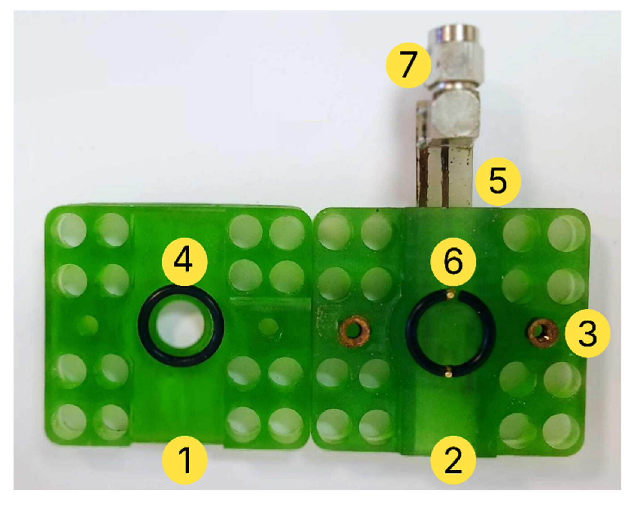
Figure 3. Temperature control and frequency acquisition unit (CA). CA1) TEC1-12706 Peltier cell. CA2) CPU fan with aluminum heatsink (12 V, 0.6 A). CA3) Raspberry Pi Pico microcontroller. CA4) NTC 3950 thermistor. CA5) VNH2SP30 H-bridge motor driver. CA6) Switching Power Supply. CA7) NanoVNA-H. 12 V. CA8) Fans.

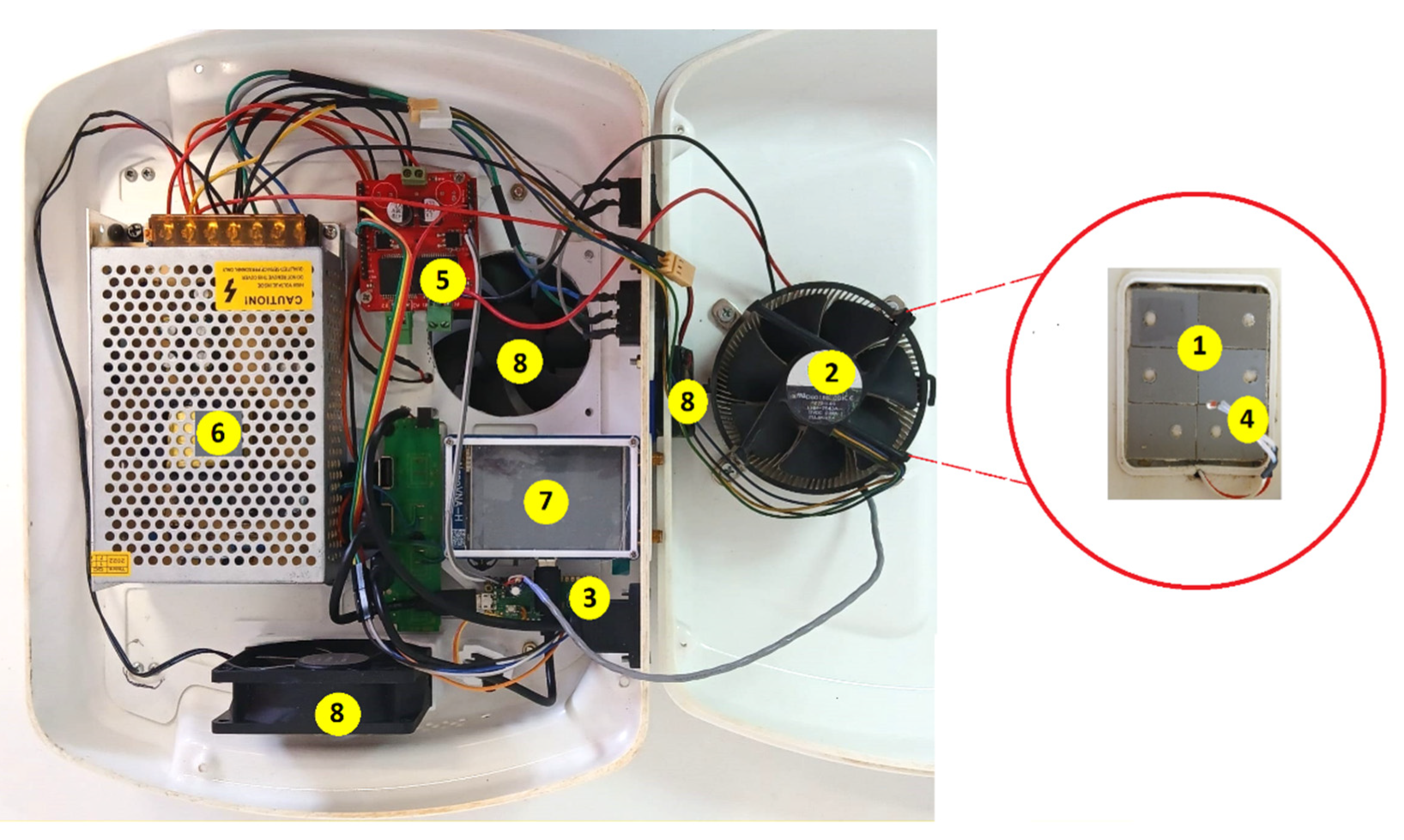
Figure 4. Overview of the customized software and its components. (A) The configuration panel displays real-time data from the active sweep and provides access to tools for setting sweep parameters, adjusting marker positions, connecting the NanoVNA device, modifying visualization options, calibrating the instrument, and exporting data. (B) The real-time output section presents a graph of f_r as a function of time, along with marker information. A reset option is included to remove all calculations and clear the temporal plot. (C) The graph displays section shows conductance curves, which are used to evaluate the performance of the sensor, with a focus on f_r and D behavior.

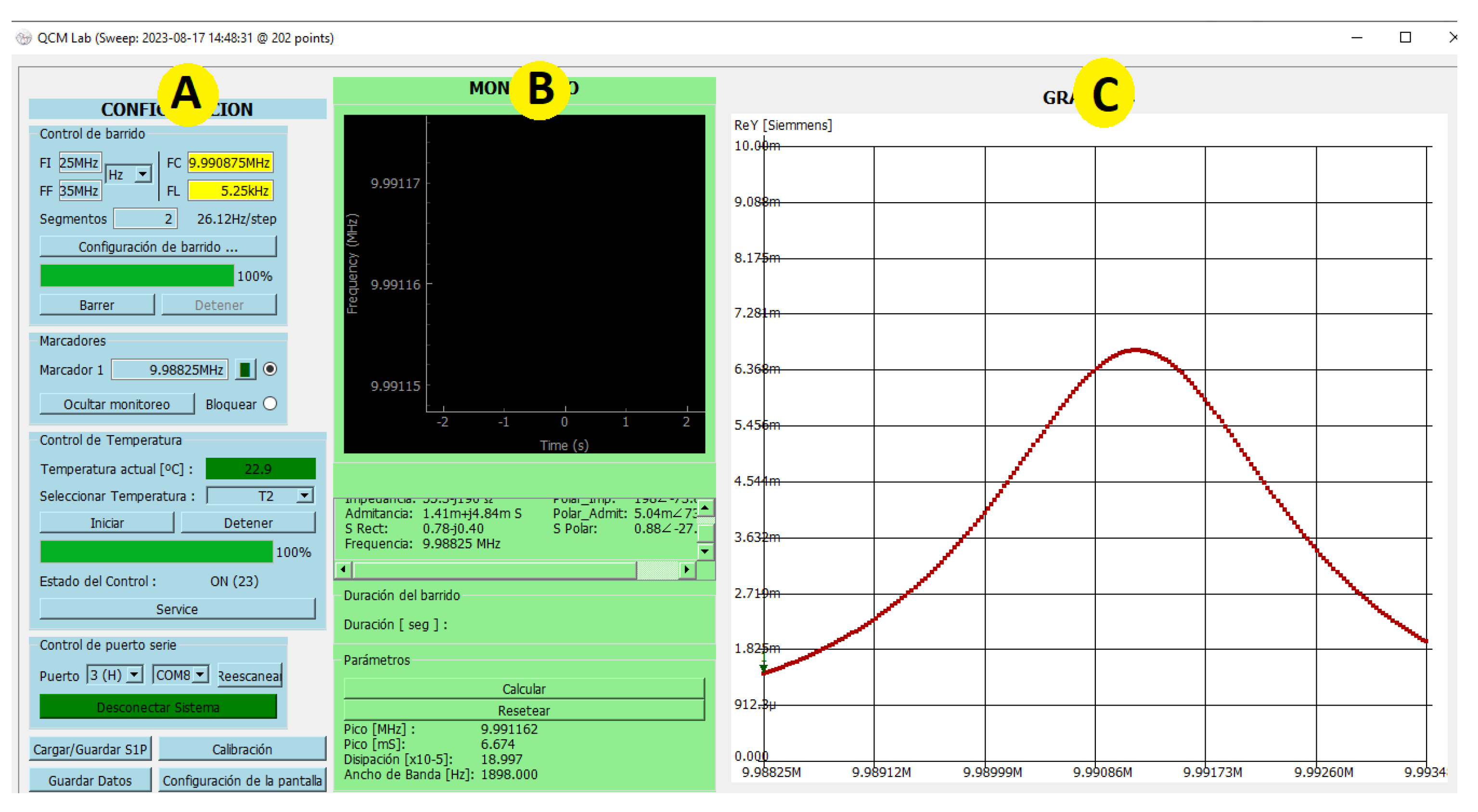
Figure 5. Housing and accessories. E1) Housing. E2) Internal base housing. E3) Top holder. E4) Fan bracket. E5) Protective cover. E6) VNA port cover. E7) Back fan trim. E8) Vent cover. E9) Legs.

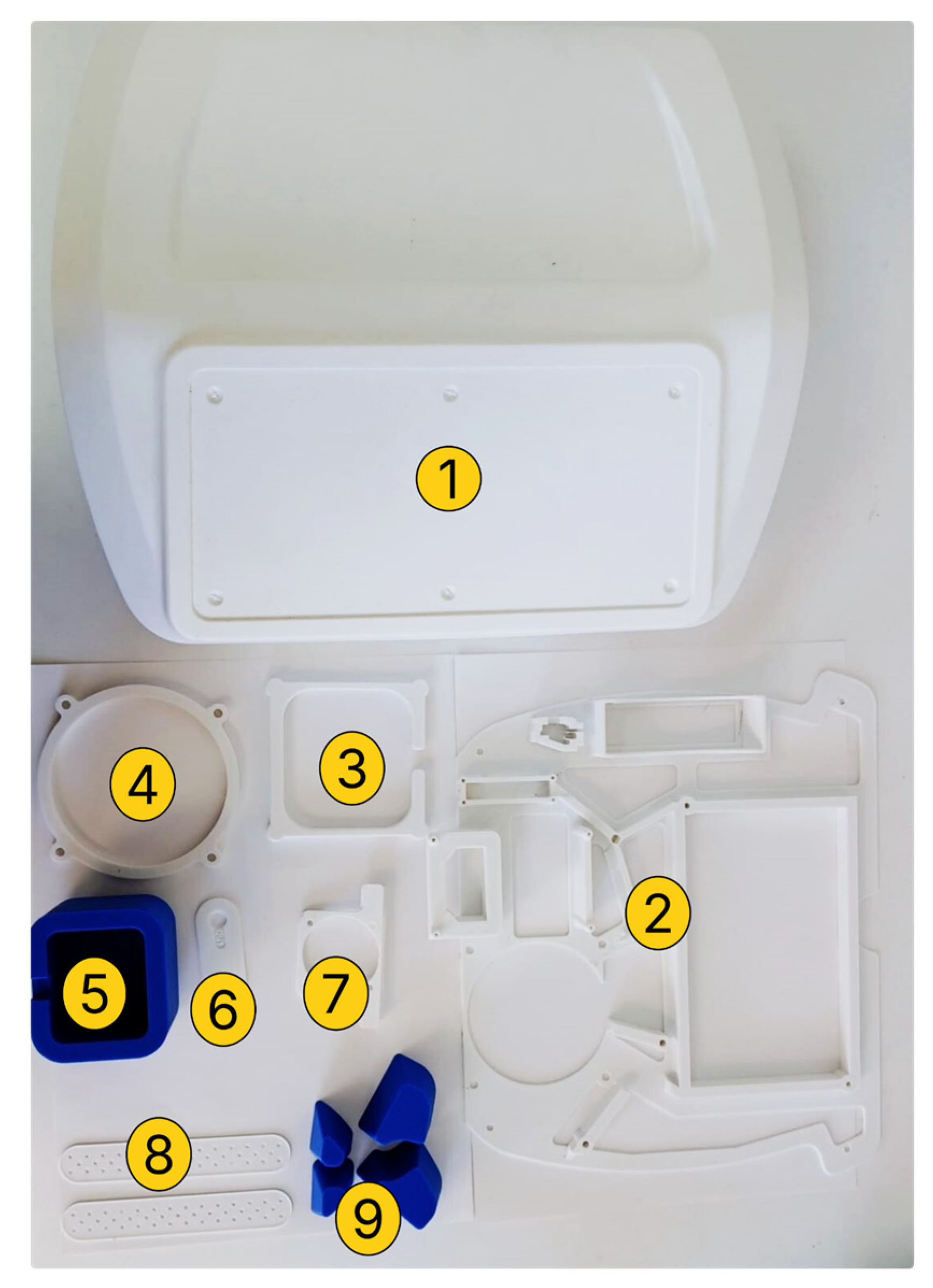
Figure 6. Mode batch. The sample is deposited directly onto the crystal using a micropipette, without circulation.

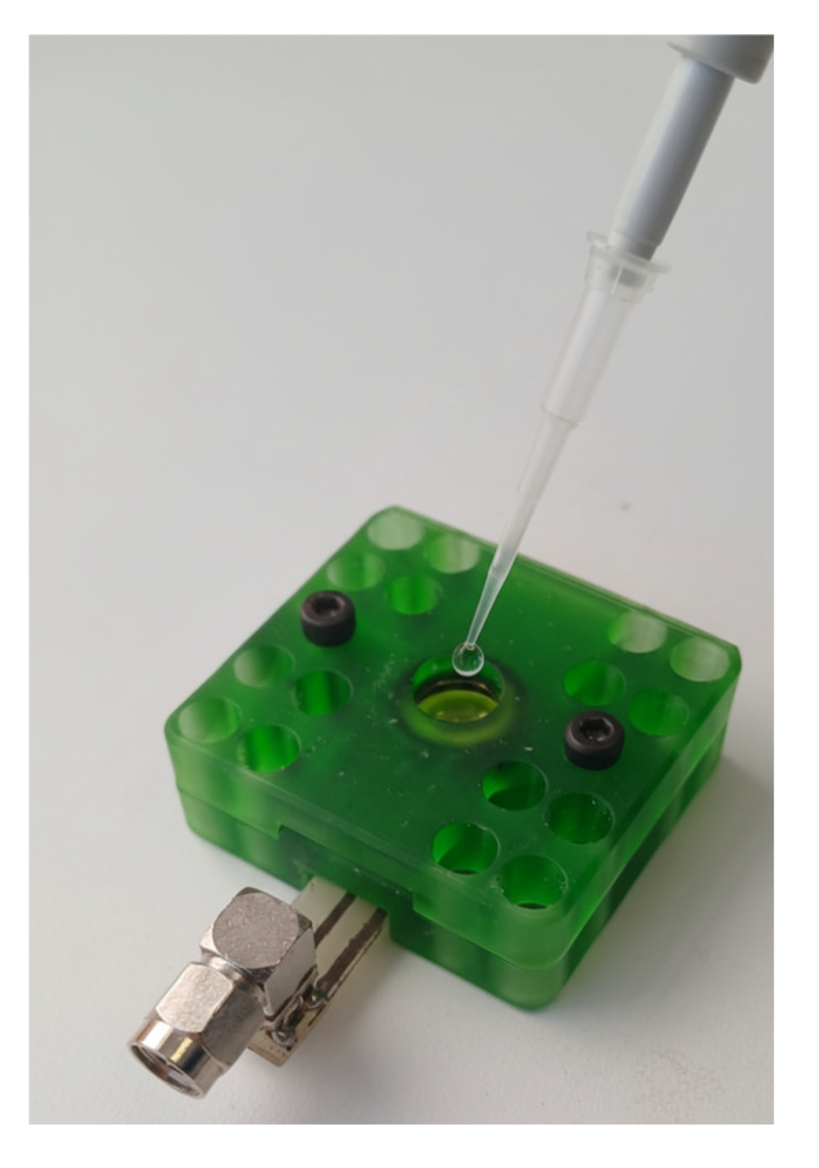
Figure 7. Crystal cleaning procedure. The crystal is immersed in a 2% SDS detergent solution for 5 minutes (A), then thoroughly rinsed with distilled water (B), and dried with pure nitrogen gas (C).

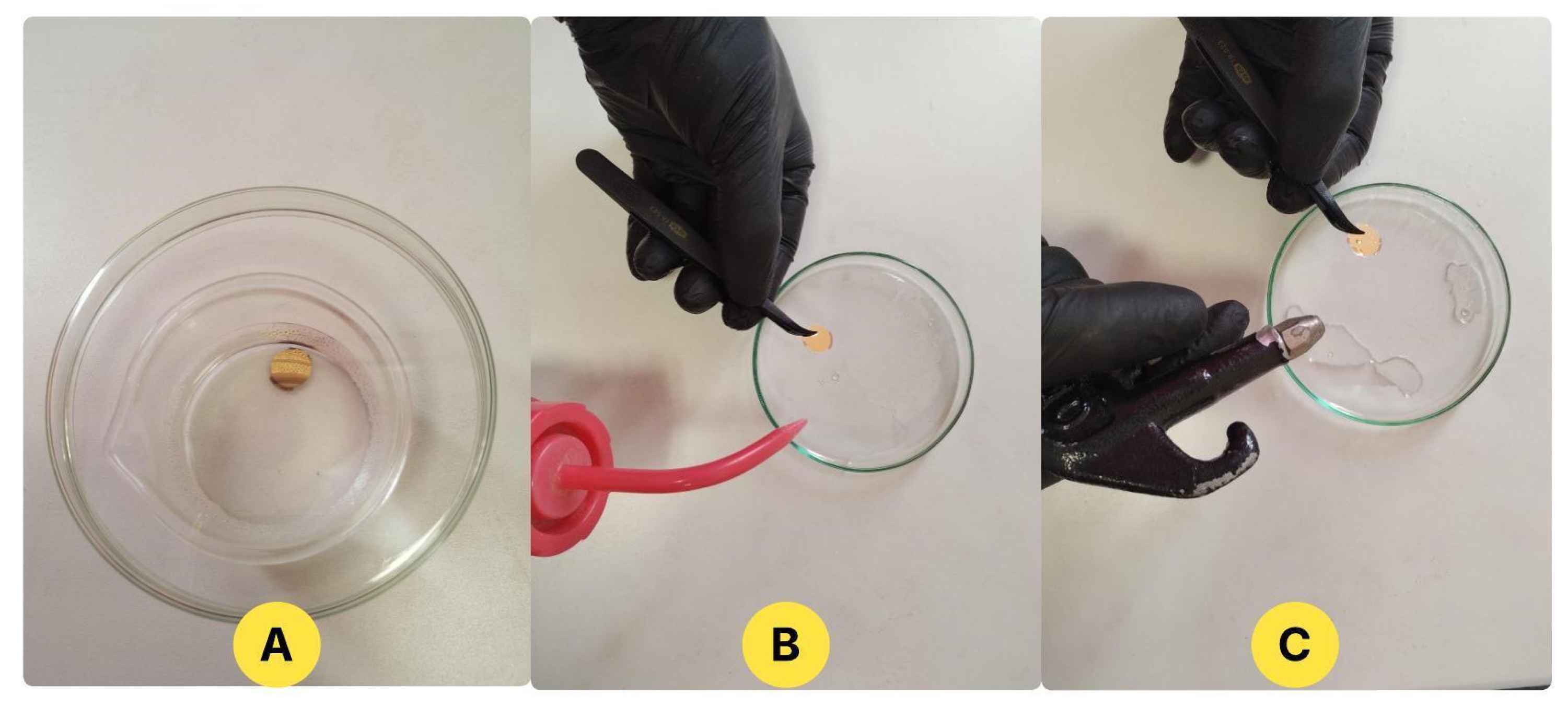
Figure 8. Temperature vs. time profile. The system shows fast response to setpoint changes and maintains temperature with minimal fluctuation during steady-state intervals.

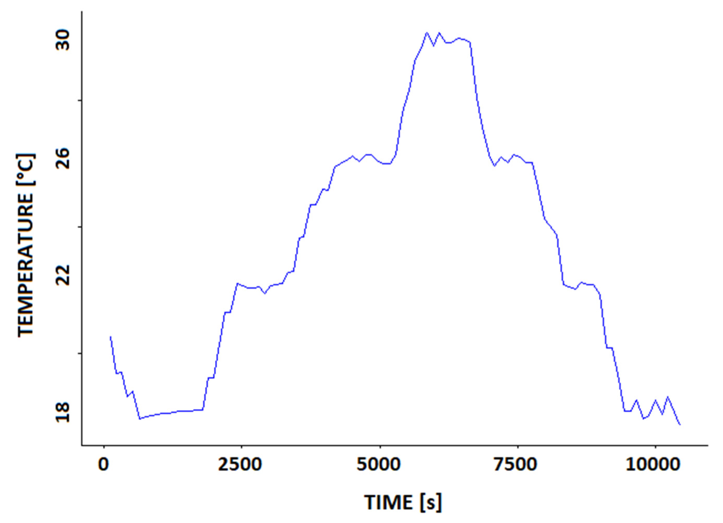
Figure 9. Frequency and dissipation shifts for distilled water and PEG solutions (2%, 5%, 10%) measured over three consecutive days at 26 °C. Bars indicate mean ± SD (n = 20 per condition).

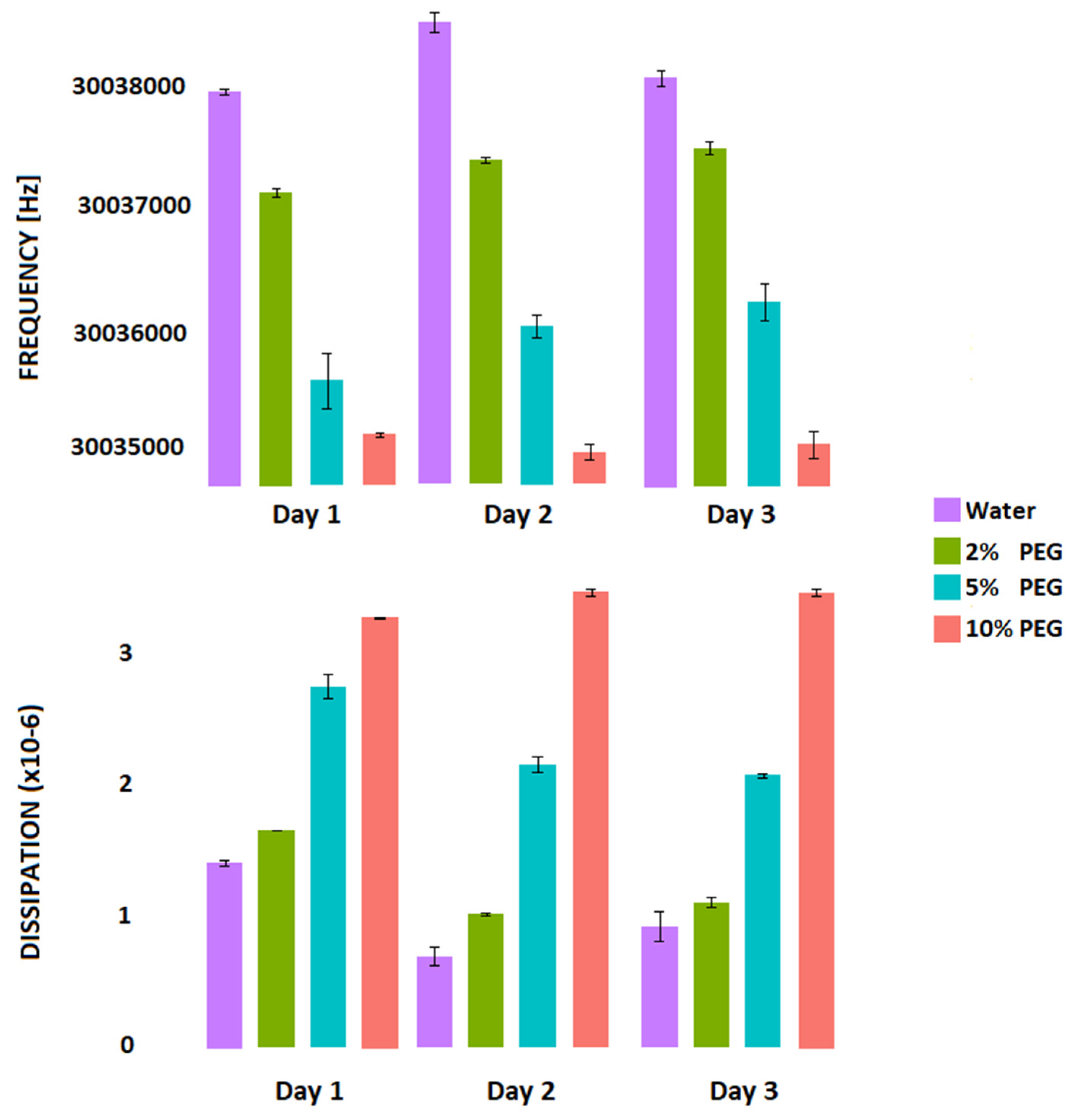
Figure 10. A clear monotonic trend was observed, demonstrating that the sensor reliably detects variations across the tested range. Sensitivity analysis was conducted using data from one representative experimental day, selected based on consistent sensor performance and thermal stability throughout all tested PEG concentrations.

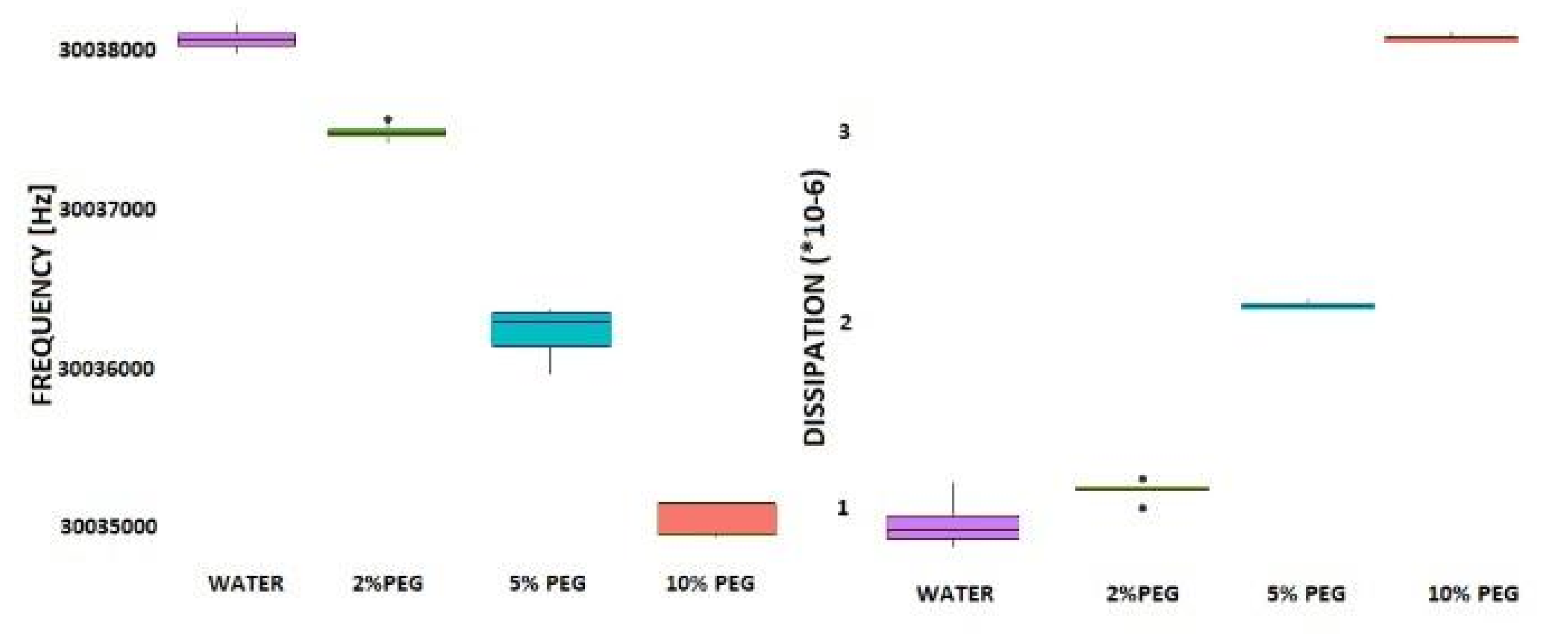
Table 3. Temperature stabilization times and steady-state values during the thermal cycling steps.

Temperature Step [°C]	Stability Time [s]	Stable Temp. (mean ± SD) [°C]
18	639	18.12 ± 0.08
18 to 22	626	22.12 ± 0.10
22 to 26	950	26.12 ± 0.13
26 to 30	560	29.93 ± 0.15
30 to 26	336	26.12 ± 0.13
26 to 22	560	22.12 ± 0.12
22 to 18	448	18.19 ± 0.27

Disclaimer/Publisher’s Note: The statements, opinions and data contained in all publications are solely those of the individual author(s) and contributor(s) and not of MDPI and/or the editor(s). MDPI and/or the editor(s) disclaim responsibility for any injury to people or property resulting from any ideas, methods, instructions or products referred to in the content.

© 2025 by the authors. Licensee MDPI, Basel, Switzerland. This article is an open access article distributed under the terms and conditions of the Creative Commons Attribution (CC BY) license (http://creativecommons.org/licenses/by/4.0/).

Copyright: This open access article is published under a Creative Commons CC BY 4.0 license, which permit the free download, distribution, and reuse, provided that the author and preprint are cited in any reuse.