
Submitted:
29 September 2025
Posted:
30 September 2025
You are already at the latest version
Abstract
Mining activities are conducted to extract valuable minerals from the Earth, used in the manufacture of many objects. However, these operations have been associated with significant landform alterations, such as deep excavations, artificial embankments, and landscape reshaping. In this study, remote sensing (RS) and geographic information systems (GIS) techniques were applied to verify landform changes induced by open-pit mining in Mazapil, Zacatecas, Mexico. Multi-temporal Landsat 5 and 8 satellite images, along with digital elevation models (DEMs) from 1998 and 2014, were used to detect variations in land cover and terrain shape. Analyses revealed ground depressions greater than −333 m and waste accumulations greater than +152 m, with an average standard deviation of ±3.6 m. A total excavation volume of 413,524,124 m³ and an embankment volume of 431,194,785 m³ were quantified, with an estimated standard deviation of ±810 m³. Despite limitations related to DEM resolution, data availability, and restricted mine access, the proposed method proved effective for the remote quantification of large-scale topographic alterations in open-pit mining areas. The integration of satellite imagery, multi-temporal DEMs, and geospatial analysis constitutes a cost-effective and replicable methodology for environmental monitoring, landscape modeling, and hydrological risk assessment in both active and post-mining environments.
Keywords:
mining
; landform
; remote sensing
; gis
; environmental monitoring
The study reveals that mining activities in Mazapil, Zacatecas,
Mexico, have caused significant changes in the terrain, with ground depressions
greater than -333 m and waste accumulations greater than +152 m.
Remote sensing (RS) techniques were used, with multi-temporal
Landsat 5 and 8 images, as well as Digital Elevation Models (DEM) from 1998 and
2014.
The analysis quantified a total excavation volume of 413,524,124
m³ and an embankment volume of 431,194,785 m³, with an estimated standard
deviation of ±810 m³.
Despite limitations related to DEM resolution and data
availability, the method used proved to be effective for remote quantification
of large-scale topographic alterations.
1. Introduction
Mining is one of the most important economic activities globally, enabling the extraction of minerals and materials essential for the manufacture of many products. However, mining operations generate a series of negative physical, environmental, and social impacts [1,2]. Among the most obvious effects are direct alterations to the Earth's crust, such as excavations, accumulation of waste material, and tailings dams, which cause deforestation, erosion, modification of natural hydrology, and the generation of solid and liquid toxic waste [3,4]. These mining wastes can contaminate the air, soil, and water if not properly treated [5,6].
Due to mining-induced impacts, extensive research has been conducted worldwide. Studies conducted in Africa, Europe, and Asia have shown that multi-temporal satellite imagery, DEMs, photogrammetric techniques, and other sensors can effectively detect landscape disturbances, changes in water bodies, and changes in vegetation cover [7,8,9,10]. For example, [7] assessed environmental changes in southwestern Sierra Leone, West Africa, using multi-date Landsat infrared imagery, complemented by field hydrological and biophysical data, to monitor the temporal and spatial dynamics of mining area features. [8] evaluated the use of multi-temporal Landsat 5 and 7 imagery, Panchromatic SPOT (Satellite Pour l'Observation de la Terre) data, and ASTER (Advanced Spaceborne Thermal Emission and Reflection Radiometer) data to map the natural environment and assess the impact of mining activities on land and water resources in Greece. [11] conducted a first-order risk assessment in the Witwatersrand Basin in South Africa to help identify vulnerable land use in the vicinity of gold and uranium mining, generating risk maps using RS and GIS. [12] evaluated the use of DEMs from the Shuttle Radar Topography Mission (SRTM) and ASTER space-based missions to identify changes in local topography and surface hydrology around the Geita gold mine in Tanzania. [13] assessed environmental conditions and developed a monitoring system for potential areal and perimeter changes in acidic lakes in the Canakkale open-pit lignite mining area in Turkey, using RS at the regional scale. More recent approaches have integrated machine learning (ML) algorithms with RS and GIS, to perform automatic and scalable assessments of mining-driven transformations. In this direction [10], they performed large-scale automatic detection of open-pit mining areas by integrating multi-temporal DEMs and multi-spectral images, using object analysis and the “Random Forest” algorithm in Inner Mongolia, China. [9], investigated on the environmental impact of underground coal mining at the Bogdanka mine, Poland, using spectral indices, satellite radar interferometry, GIS tools, and ML algorithms, from optical, radar, geological, hydrological, and meteorological data, to develop a spatial model and determine the statistical significance of the individual impact of factors related to the presence of wetlands. In Mexico, efforts have been made to assess the environmental externalities associated with mining activities, such as those observed at the Peñasquito mine in Mazapil, Zacatecas, where land use change, vegetation loss, and groundwater dynamics have been analyzed [14].
Conventional land surveys, which previously relied on mechanical instruments such as theodolites, tape measures, and leveling devices [15], have been replaced by robotic total stations, Global Navigation Satellite Systems (GNSS), terrestrial laser scanners, and Light Detection and Ranging (LiDAR) sensors [16,17]. However, these methods are often limited by high operational costs and limited temporal coverage. In contrast, recent advances in RS, including airborne and satellite photogrammetry and radar interferometry [18,19,20], have enabled continuous, large-scale, and non-invasive monitoring of terrain morphology, offering an effective alternative to traditional ground-based measurements. Despite these advances, satellite information has been underutilized due to a lack of awareness of its potential and its limitations related to geometric resolution. However, for environmental monitoring in mining areas, satellite imagery is a highly cost-effective and replicable technique.
Within this framework, the overall objective of this study was to detect and measure mining-induced relief alterations in Mazapil, Zacatecas, Mexico, using satellite imagery and GIS processing. This approach was designed to overcome the limitations of field surveying by combining multi-temporal satellite imagery and DEMs to detect relief changes and estimate material extraction volumes.
2. Materials and Methods
2.1. Study Area
This research was conducted in a mining region located in the municipality of Mazapil, in the state of Zacatecas, Mexico. The study area is geographically located between latitudes 24°33'57.57" and 24°42'14.56" north, and between longitudes 101°50'45.10" and 101°27'10.32" west (Figure 1). This area is part of two physiographic provinces: the Sierra Madre Occidental (52.7%) and the Mesa del Centro (47.3%), which include the sub provinces of Sierras Transversals and Río Grande [21].
Mazapil is characterized by a highly variable landform that includes flat terrain, peaks, ridges, slopes, and valleys. Elevations range from 1,300 to 3,200 meters above mean sea level. The climate is classified as dry temperate, semi-dry temperate, very dry semi-warm, and semi-cold sub-humid, with a mean annual temperature of approximately 17 °C and annual precipitation between 200 and 600 mm, concentrated during the summer months. The dominant vegetation cover consists of shrubland (95.28%), forest (1.68%), grassland (0.90%), mesquite woodland (0.04%), and areas with no clear vegetation (0.09%) [21].
Mazapil is located within the Mexican Silver Belt, one of the most important metallogenic provinces in the country, home to large poly-metallic deposits of gold, silver, lead, and zinc [23]. This mineral wealth has driven the development of large open-pit mining complexes, including the Peñasquito Mining Unit, whose open-pit operation has generated significant transformations in the terrain through excavations, waste dumps, tailings dams, and haul roads [14].
2.2. Methodology
A mixed-methodological approach was implemented, integrating quantitative techniques for the analysis of altimetric differences and volumetric estimation, and a qualitative approach for the characterization of landforms. This strategy was designed based on the general methodology for change detection proposed by [24] and incorporating change detection and classification techniques such as those described by [25]. The method is structured into five stages:
- Acquisition of satellite images and DEM.
- Radiometric and geometric corrections and information preparation.
- Change detection and analysis.
- Evaluation of the reliability of the obtained data.
- Generation of results.
This methodology provides a replicable workflow, allowing the integration of RS and GIS techniques to assess the physical impacts of mining on the landscape.
2.2.1. Acquisition of Satellite Images and DEMs Before and After Mining Activity
In the first stage, multi-temporal satellite images were acquired from 1998 and after the development of mining activity in 2014. The images were obtained from the medium-resolution Landsat 5 and Landsat 8 satellites, widely recognized for their reliability in environmental monitoring. To extract altimetric information, DEMs were acquired from various sources, such as the National Institute of Statistics and Geography (INEGI) from 1998, the ASTER satellite from 1999, the SRTM space mission from 2000, the Advanced Land Observing Satellite (ALOS PALSAR) from 2006, and the Copernicus mission from 2011 to 2015, with a geometric resolution of 15, 30, 30, and 17 m, respectively. All data was downloaded from official websites such as INEGI, the United States Geological Survey (USGS), Copernicus Browser, and the National Aeronautics and Space Administration (NASA). These data sets provide us with temporal and redundant information for statistical analysis of the errors and standard deviation of the detected elevation differences.
2.2.2. Radiometric and Geometric Corrections and Preparation of Satellite Images and DEM
Satellite image preprocessing included radiometric and geometric corrections, as well as the transformation of the datasets to the WGS84 UTM reference coordinate system, Zone 14 North. This process was performed using GIS software QGIS v3.40.5, ensuring homogenization and spatial compatibility of the inputs. For radiometric corrections, the conversion from Digital Numbers (DN) to Upper Atmospheric Reflectance (TOA) was performed using the standard equation provided by the data source [26]. This step allowed for the normalization of pixel values, reducing the influence of atmospheric conditions, sensor-specific differences, and acquisition dates, thereby improving the comparability of the multitemporal images. The DEMs were projected to the WGS84 UTM Zone 14 North reference coordinate system to obtain coordinates in meters. They were interpolated to a pixel resolution of 15x15 m to ensure uniformity and subsequently cropped to the extent of the mining area of interest.
In this preprocessing stage, the reflectance values of the satellite images were calibrated, the DEMs were interpolated to the same pixel resolution, the dataset was projected to the same reference coordinate system and cropped to the extent of the area of interest. This homogenization of the dataset allowed for pixel-to-pixel correspondence, an essential requirement for the subsequent detection of changes in relief and for volumetric calculation.
2.2.3. Detection of Changes in Satellite Images and DEMs
To visualize changes in the mining area using satellite imagery, combinations of Shortwave Infrared (SWIR), Near Infrared (NIR), and Red bands were used. This false-color band combination is used for vegetation analysis and shows greater differences between soil, vegetation, and water bodies [27].
The monitoring of relief changes in the mining area was conducted by classifying the different relief forms before and after mining activity. The relief type classification method was based on the approach proposed by [28], which allows for the segmentation of relief types from the DEM. This process facilitated the identification of significant geomorphological transformations due to mining operations.
Topographic changes were detected using the Difference DEM technique. A pixel-by-pixel algebraic subtraction was performed between the 2014 Copernicus DEM [29] and the 1998 INEGI DEM [30], the 1999 ASTER DEM [31], and the 2000 SRTM DEM [32]. This procedure generated elevation change detection maps and allowed for the correct delineation of excavation and waste material accumulation zones.
In addition, pixel-by-pixel excavation and fill volumes, as well as total volumes for the area of interest, were calculated. The grid method was applied to calculate the volume (equations 1, 2, and 3), which consists of calculating the area of each pixel and multiplying it by the excavation thickness (negative sign) or fill (positive sign). This method, adapted from [15,33], provided a quantification of the volumetric changes associated with mining-induced relief alterations.
∆ Elevations =Recent DEM - Oldest DEM,
Pixel area = (DEM resolution)2,
Volume = Pixel area× ∆ Elevations,
The negative values of Delta Elevation were interpreted as excavation zones, while positive values corresponded to fill zones. These equations allowed for pixel-by-pixel estimation of excavation and fill volumes across the study area, ensuring accurate quantification of topographic changes resulting from mining activities.
2.2.4. Evaluation of Data Reliability
The results obtained were validated by visually comparing Landsat 5 and Landsat 8 images with historical topographic maps from the INEGI (National Institute of Statistics and Geography). The positional and altimetric accuracy of the DEMs was also evaluated by calculating root mean square (RMS) errors. Basic statistical analyses were applied to verify the spatial consistency of the results and reduce the margin of error in interpretation.
To measure the magnitude of the differences between the DEMs, a comparison was made, and the Vertical Error (∆h), Mean Error (ME), Standard Deviation (SD), and Root Mean Square Error (RMSE) were calculated pixel by pixel [34]. The INEGI DEM was considered the true value, as it is a model obtained with aerial photogrammetry, field information, and higher resolution, using the following equations:
Error Vertical (∆h):
Where ∆h is the vertical error of a measurement is, DEMx is a digital elevation model x and DEMINEGI is the INEGI DEM.
Mean Error (ME):
Standard Deviation (SD):
Root Mean Square Error (RMSE):
2.2.5. Generation of Final Maps of Terrain Alterations
Finally, cartographic products were generated to represent the main relief alterations induced by mining, including comparative maps of Landsat images, elevation difference maps, and volume maps. The maps were generated from the collected dataset and processed using different algorithms in QGIS v3.40.5 software. This methodology represents an efficient, replicable, and low-cost alternative to traditional field methods and constitutes a strategic tool for the continuous monitoring of the morphological impact in regions affected by mining activities.
3. Results
3.1. Vertical error, standard deviation, and mean square error for the different DEM.
The ALOS, ASTER, and SRTM DEMs were compared with the INEGI DEM on a pixel-by-pixel basis, and then the average across all pixels was obtained. Table 1 presents a summary of the results for the mean vertical error, mean standard deviation, and mean square error.
The ASTER-INEGI and SRTM-INEGI DEMs present mean vertical errors (ME) close to zero (1,259 m and 1,272 m, respectively), showing strong altimetric agreement. In contrast, the ALOS DEM displays a significant negative mean vertical error (-14,420 m), reflecting a systematic bias associated with differences in elevation reference surfaces. The standard deviation (SD) and root mean square error (RMSE) further support this pattern: ASTER (SD = 8,560 m; RMSE = 8,652 m) and SRTM (SD = 6,372 m; RMSE = 6,498 m) present moderate variability and adequate alignment for the study area, whereas ALOS (SD = 5,685 m; RMSE = 15,501 m) combines relatively low dispersion with pronounced vertical bias. This behavior justifies the exclusion of the ALOS DEM from the final analysis.
3.2. Detection of Physical Changes in the Mining Area Using Satellite Images and DEMs
3.2.1. Detection of Changes in Satellite Images
To identify physical changes induced by mining activities in the Mazapil region, false-color composites of multispectral bands were employed. Bands 5, 4, and 3 of Landsat 5 (1998) and bands 6, 5, and 4 of Landsat 8 (2014) were used. This spectral configuration is widely recognized for vegetation analysis, detection of exposed surfaces, and identification of water bodies (Figure 2). In these composites, vegetation is shown in various shades of green, urban areas and bare soil appear in shades of pink, and water bodies are represented in black and light blue [27].
3.2.2. Detection of Relief Changes Using Multitemporal DEM.
The detection of mining-induced relief alterations was conducted by classifying relief types for the years 1998 and 2014, comparing pre- and post-mining conditions. The method applied was based on the approach proposed by [28], which uses a computer vision algorithm to calculate Geomorphons (landforms) and their associated geometry. For this study, multiple tests were conducted with variable search radio, and the best results were obtained using an outer radius of 30 units, an inner radius of 15 units, and a flatness threshold of 2°. This configuration resulted in a classification of the terrain into the following relief types: flat, peak, ridge, shoulder, spur, slope, hollow, toe of slope, valley, and pit [28].
As illustrated in Figure 3, in 1998, the study area was dominated by flat surfaces and gentle slopes, with minimal evidence of anthropogenic alteration. However, the 2014 classification reveals the appearance of large depressions (pits) in the central sector, accompanied by the formation of artificial mounds visible as newly developed ridges and shoulders, resulting from excavation activities and spoil deposition. These transformations are particularly evident in the vicinity of the open-pit mine, where the flat areas have been replaced by extensive depressions and the surrounding terrain has been reshaped into raised spoil piles. These changes are of such magnitude that they are clearly detectable from space, demonstrating the ability of remote sensing and Geomorphons-based classification to capture large-scale geomorphological transformations.
3.2.3. Detection of Elevation Changes Using Multi-Temporal DEMs
To detect mining-induced land elevation changes, multitemporal DEMs obtained from diverse sources were used. The procedure consisted of performing pixel-by-pixel algebraic subtraction between the 2014 Copernicus DEM and three historical DEMs: the 1998 INEGI DEM, the 1999 ASTER DEM, and the 2000 SRTM DEM. This analysis allowed us to identify the accumulated altimetric differences between 1998 and 2014 (Figure 4).
Figure 4 shows consistent spatial patterns of relief alteration, directly associated with areas of intense mining activity. Negative elevation differences, reaching −318 m with Copernicus-INEGI, −320 m with Copernicus-SRTM, and −323 m with Copernicus-ASTER, are represented in blue, green, and yellow shades, showing deep excavations such as open-pit mines. Conversely, positive elevation changes, up to +128 m in Copernicus–SRTM, +133 m in Copernicus–INEGI, and +130 m in Copernicus–ASTER, appear in orange and red tones, corresponding to waste rock piles and tailings dams created during mining operations.
3.3. Evaluation of the Reliability of Elevation Differences through Standard Deviation Analysis
To assess the reliability and spatial consistency of the elevation difference data, three topographic change maps were generated for the DEM pairs Copernicus–INEGI, Copernicus–ASTER, and Copernicus–SRTM (Figure 4). This redundancy provided a robust comparative basis between DEMs derived from diverse sources and spatial resolutions. The variability was quantified using pixel-by-pixel standard deviation (SD) calculations across the three different maps. For this analysis, the Copernicus–INEGI model was considered the “reference dataset,” due to its higher spatial resolution and generation from aerial photogrammetry supported by field-based topographic control, thereby ensuring superior cartographic accuracy. Based on this reference, the standard deviation map shown in Figure 5 was produced.
The map reveals that most of the study area is characterized by SD values ≤12 m (green), which correspond primarily to flat or gently sloping surfaces, where the three DEMs exhibit strong altimetric agreement. Moderate SD values, between 12 and 25 m (yellow), are observed in areas with intermediate slopes, while the highest SD values >25 m (red) are sparsely distributed and concentrated in mountainous areas, especially along ridgetops and steep slopes. This spatial distribution shows that the greatest altimetric discrepancies between DEMs are associated with steep topographic gradients, where interpolation and sensor-related geometric errors are most likely to occur.
3.4. Generation of the Final Maps
3.4.1. Average map of Topographic Alterations in the Mining Area
To reduce the uncertainty associated with differences between digital elevation models (DEMs) derived from various sources, an average map of topographic alterations was generated for the study area. This map was produced by calculating the pixel-by-pixel arithmetic meaning of the three elevation difference maps previously obtained: Copernicus-INEGI, Copernicus-ASTER, and Copernicus-SRTM, which were presented in Figure 4.
The result of this integration is shown in Figure 6, where the cumulative average elevation differences between 1998 and 2014 are represented. The color scale is sequential, where dark tones (violet and blue) indicate the greatest reductions in elevation (≤ −320 m), corresponding to deep excavation zones, while orange and red tones represent increases in elevation (> +129 m), associated with mine waste accumulation or tailings dam construction.
As seen, the areas with the most intense topographic changes are concentrated in the middle part of the map, where the main pits and mining deposits are found. These zones show maximum excavation depths of −361 m, showing a considerable volume of material removed from the subsurface during the analysis period. In contrast, artificially elevated regions, with a maximum increase of +170 m, were found and are linked to waste rock storage zones.
3.4.2 Delimitation of the active mining area
Complementarily, the active mining activity polygon was delineated based on the visual interpretation of the Landsat 8 satellite image obtained on February 5, 2014 (Figure 7). This polygon was traced using the visible boundaries of open-pit mines, tailing dams, artificial water bodies, and haul roads. The overlay of this mining zone on the altimetric analysis products allowed for the spatial validation of the correspondence between the areas showing the greatest topographic alterations and the geographic footprint of industrial mining.
3.4.3. Elevation Changes within the Mining Footprint
To isolate only the topographic changes directly associated with mining activity, the average elevation difference map was cropped using the polygon corresponding to the delimited mining area as a mask (Figure 7). The results are presented in Figure 8, which shows only the elevation changes that occurred within the mining perimeter.
Figure 8 shows substantial transformations in the natural terrain. Areas shaded from dark blue to yellow represent deep excavations, with elevation losses greater than −333 m relative to the original terrain, while areas ranging from orange to deep brown correspond to waste deposits, where an elevation increase of more than +152 m has been recorded. These values confirm a drastic modification of the landscape, consistent with the removal and accumulation patterns characteristic of large-scale open-pit mining.
Table 2 presents quantitative data on the area affected by elevation changes within the mining zone. The deep excavation area covers 2,587 km2, the moderately or undisturbed areas cover 29,281 km2, and the area affected by mining waste dumping is 12,632 km2.
3.4.4. Calculation of Excavation and Filling Volumes Within the Mining Area.
Based on the average map of relief alterations, the total volume of excavated material (cut) and accumulated material (fill) within the mining polygon was calculated. The procedure involved computing the volume of each pixel by multiplying its area by the corresponding elevation difference. This approach was adapted from methodologies proposed by [15,33]. The spatial result of the volume calculation is presented in Figure 9, showing volumetric variations distributed within the mining area, expressed in cubic meters per pixel.
The highest excavation zones are concentrated in the northeast sector of the polygon, reaching unit volumes greater than −71,940 m³ per pixel, while the largest fill values exceed +30,985 m³ per pixel in tailings dam and deposition platform areas. Subsequently, a summation of all negative (excavation) and positive (fill) pixel values yielded a total excavation volume of 413,524,124 m³ and a total fill volume of 431,194,785 m³. To incorporate the uncertainty associated with the elevation differences used in the calculation, an average standard deviation of ±3.6 m (obtained in section 3.3) was considered. From this, an estimated volumetric standard deviation of ±810 m³ was calculated as the expected variability threshold in the volumetric estimates per pixel (Table 3).
4. Discussion
Detecting land cover and land use changes using satellite imagery is a technique that has been widely used in various research projects [41,42,43,44]. Therefore, this study used multi-temporal imagery to detect land cover and land use changes. For example, Figure 2 (a) from February 9, 1998, shows natural vegetation and soil cover due to limited mining activity in the study area. In contrast, Figure 2 (b) from February 5, 2014, shows a marked transformation of the landscape. Large areas of bright pink and light blue dominate the central part of the image, corresponding to tailing dams, artificial water bodies, and active mining areas.
Multi-temporal DEMs were used to detect landform changes, as Landsat images do not provide terrain elevation information. Therefore, the different landform classes were obtained according to the classification by [28] between 1998 and 2014. This allowed for the observation of anthropogenic changes in the landscape and can assist in the planning of rehabilitation of affected lands.
These landform changes were measured through elevation changes between 1998 and 2014, using the multi-temporal DEMs in Figure 4. The maximum negative elevation differences were -361 m, represented in shades of blue, green, and yellow, associated with deep excavations. On the other hand, the maximum positive elevation changes were +170 m, appearing in orange and red hues, corresponding to waste rock piles and tailing dams. Similar alterations have been documented in other mining regions around the world. These include those reported by [12], who detected topographic changes greater than -250 m at the Geita gold mine in Tanzania using multi-temporal DEM differences. Similarly, [10] reported elevation variations between -258 m and +162 m in Inner Mongolia associated with large-scale open-pit mining. The results obtained in Mazapil and elsewhere around the world reinforce the validity of the method and reveal its applicability to diverse mining sites.
These results clearly illustrate the physical impact of open-pit mining on the local topography in less than two decades. The magnitude of the detected altimetric differences shows substantial volumes of removed material, which not only reshapes the original landscape but also has the potential to change hydrological processes, erosion dynamics, and surface runoff patterns.
To assess the reliability of the detected altimetric differences, the standard deviation (SD) of the three generated maps was calculated. The generated SD map shows that the largest altimetric discrepancies between the DEMs are associated with steep topographic gradients, where interpolation, geometric, and sensor-related errors are more likely to occur. The average SD for the entire study area was ±3.6 m, a value considered statistically low for regional-scale elevation change studies. Previous evaluations of the SRTM DEM have reported vertical errors of ±10 m for lowlands and up to ±36 m in mountainous regions [37]. Similarly, ASTER DEMs shows errors ranging from ±7 m to ±26 m depending on elevation and topography [38]. The accuracy of DEMs varies considerably depending on the terrain type and product used, so it is essential to consider these margins of error when interpreting and using the data in scientific or land management applications.
From the three elevation difference maps obtained, an average elevation difference map was created to smooth out possible local errors present in the individual models and improve the spatial representation of actual topographic changes. This approach has been used in previous studies with similar purposes. For example, [36] compared and examined the accuracy of six freely available global DEMs (ASTER, AW3D30, MERIT, TanDEM-X, SRTM, and NASADEM) in four geographic regions with different topographic and land-use conditions. They used high-precision local elevation models (LiDAR and Pleiades-1A) as reference models. They estimated the accuracy by generating error raster’s by subtracting each reference model from the corresponding global DEM and calculated descriptive statistics such as mean, median, and root mean square error (RMSE) for this difference.
Since not all relief changes correspond to mining activities, the mining area was delimited by a polygon, covering approximately 44.5 km² and encompassing all associated mining infrastructure. In particular, the tailings dam covers almost 4.9 km², while the main excavation area of the pit occupies approximately 2.5 km². This spatial correlation reinforces the validity of the altimetric change detection results, demonstrating that the areas of greatest elevation loss and gain accurately correspond to the operational footprint of mining activities.
After delineating the mining area, the volume of excavation and fill was calculated. The method used has been validated in other international studies on open-pit mining. For example, [39] conducted a study in Central Java Province, Indonesia, to measure the extent of minerals and calculate the extracted volumes using a more ecological approach. Drones (unmanned aerial vehicles) and DEMs were used to measure and calculate the volumetric properties of the minerals, yielding volume deviations of ±768 m3. For this reason, a certain degree of error in volume calculations is normal, and they are suitable for some uses and not for others.
5. Conclusions
The applied methodology proved effective in detecting and quantifying relief changes in an active mining area by integrating satellite imagery and multi-temporal DEM. It was possible to clearly identify excavation and fill zones; calculate excavation and fill material volumes; and generate reliable geospatial products, even without access to the mine. This demonstrates the robustness of the approach for remote monitoring of large-scale mining landscapes.
However, the methodology is limited by the availability, resolution, and accuracy of DEMs for a specific date. Furthermore, the lack of access to active mines limits in-situ measurements. These restrictions must be considered when implementing this methodology in other regions or scales.
Despite these limitations, the approach is particularly suitable for open-pit mines, where relief changes are larger and more visible from satellite sensors. The application of the methodology is recommended for areas where the relief changes are greater than ±3.6 m in elevation, since smaller elevation differences may not be detected.
The integration of remote sensing and GIS offers a replicable and low-cost tool for the remote environmental assessment of mining landscapes. These methodologies can be implemented to characterize watersheds, landscapes, and geotechnical risk models in future work. Furthermore, the multi-temporal analysis demonstrated the ability to show changes over time in mining areas, roads, buildings, deforestation, and soil changes over time. These findings suggest that the technique can be adapted for continuous monitoring of mining's secondary impacts.
The findings of this research are expected to contribute to a comprehensive understanding of mining-related landscape transformations and provide a replicable and cost-effective framework to support sustainable environmental management and planning, evidence-based environmental planning, and long-term landscape restoration in mining-affected regions.
Author Contributions
Conceptualization, S.D-C. and A-G.C-M.; methodology, S.D-C. and A-G.C-M.; validation, C-F.B-C., E-D.M-V. and V-I.R-A.; formal analysis, C-O.R-R. and L-A.P-T.; investigation, S.D-C. and A.G. C-M.; data curation, S.D-C. and A.G. C-M.; writing—original draft preparation, S.D-C. and A-G. C-M.; writing—review and editing, S.D-C. and A-G. C-M.; visualization, E-D.M-V. and V-I.R-A.; supervision, A.R-T and S.I-D. All authors have read and agreed to the published version of the manuscript.” Please turn to the CRediT taxonomy for the term explanation. Authorship must be limited to those who have contributed substantially to the work reported.
Funding
This research received no external funding.
Data Availability Statement
The original contributions presented in this study are included in the article. Further inquiries can be directed to the corresponding author(s).
Acknowledgments
The authors thank the National Council for Humanities, Sciences and Technologies (CONAHCYT) of Mexico for the scholarship awarded to Master of Science Saúl Dávila Cisneros to pursue doctoral studies and generate this research.
Conflicts of Interest
The authors declare no conflicts of interest.
Abbreviations
The following abbreviations are used in this manuscript:
| RS | Remote Sensing |
| GIS | Geographic Information Systems |
| DEM | Digital Elevation Models |
| SPOT | Satellite Pour l’Observation de la Terre |
| ASTER | Advanced Spaceborne Thermal Emission and Reflection Radiometer |
| SRTM | Shuttle Radar Topography Mission |
| ML | Machine Learning |
| GNSS | Global Navigation Satellite Systems |
| LiDAR | Light Detection and Ranging |
| INEGI | National Institute of Statistics and Geography |
| ALOS | Advanced Land Observing Satellite |
| USGS | United States Geological Survey |
| NASA | National Aeronautics and Space Administration. |
References
- Werner, T.T.; Bebbington, A.; Gregory, G. Assessing impacts of mining: Recent contributions from GIS and remote sensing. The Extractive Industries and Society 2019, 6, 993–1012. [Google Scholar] [CrossRef]
- Seloa, P.; Ngole-Jeme, V. Community Perceptions on Environmental and Social Impacts of Mining in Limpopo South Africa and the Implications on Corporate Social Responsibility. Journal of Integrative Environmental Sciences 2022, 19, 189–207. [Google Scholar] [CrossRef]
- Sengupta, M. Environmental impacts of mining: Monitoring, Restoration, and Control, 2 ed.; CRC Press: Boca Raton, London y New york, 2021. [Google Scholar]
- Laker, M.C. Environmental Impacts of Gold Mining—With Special Reference to South Africa. Mining 2023, 3, 205–220. [Google Scholar] [CrossRef]
- Jiménez, C.; Huante, P.; Rincón, E. Restauración de minas superficiales en México; SEMARNAT, 2006.
- Khobragade, K. Impact of Mining Activity on environment: An Overview. International journal of scientific and research publications 2020, 10, 784–791. [Google Scholar] [CrossRef]
- Akiwumi, F.A.; Butler, D.R. Mining and environmental change in Sierra Leone, West Africa: a remote sensing and hydrogeomorphological study. Environmental Monitoring and Assessment 2008, 142, 309–318. [Google Scholar] [CrossRef] [PubMed]
- Charou, E.; Stefouli, M.; Dimitrakopoulos, D.; Vasiliou, E.; Mavrantza, O.D. Using Remote Sensing to Assess Impact of Mining Activities on Land and Water Resources. Mine Water and the Environment 2010, 29, 45–52. [Google Scholar] [CrossRef]
- Kope´c, A.; Trybała, P.; Gł ˛abicki, D.; Buczy´nska, A.; Owczarz, K.; Bugajska, N.; Kozi´nska, P.; Chojwa, M.; Gattner, A. Application of Remote Sensing, GIS and Machine Learning with Geographically Weighted Regression in Assessing the Impact of Hard Coal Mining on the Natural Environment. Sustainability 2020, 12, 9338. [Google Scholar] [CrossRef]
- Wu,Q.;Song, C.; Liu, K.; Ke, L. Integration of TanDEM-X and SRTM DEMs and Spectral Imagery to Improve the Large-Scale Detection of Opencast Mining Areas. Remote Sensing 2020, 12. [CrossRef]
- Sutton, M.W. Use of remote sensing and GIS in a risk assessment of gold and uranium mine residue deposits and identification of vulnerable land use. PhD Thesis, University of the Witwatersrand, Johannesburg, 2012. [Google Scholar]
- Emel, J.; Plisinski, J.; Rogan, J. Monitoring geomorphic and hydrologic change at mine sites using satellite imagery: The Geita Gold Mine in Tanzania. Applied Geography 2014, 54, 243–249. [Google Scholar] [CrossRef]
- Yucel, D.S.; Yucel, M.A.; Baba, A. Change detection and visualization of acid mine lakes using time series satellite image data in geographic information systems (GIS): Can (Canakkale) County, NW Turkey. Environmental Earth Sciences 2014, 72, 4311–4323. [Google Scholar] [CrossRef]
- Esparza Ramos, I.A.; Pech Canché, J.M.; Escobar León, M.C. Externalidades ambientales generadas por la Unidad minera Peñasquito, Mazapil, Zacatecas, México 2021.
- Schofield, W.; Breach, M. Engineering Surveying, 6 ed.; CRC Press, 2007.
- Kavanagh, B.F.; Slattery, D. Surveying with Construction Applications; 2014.
- Ghilani, C.D.; Wolf, P.R. Elementary Surveying. An Introduction to Geomatics, 13 ed.; Pearson Education, 2015.
- Chang,K.J.; Tseng, C.W.; Tseng, C.M.; Liao, T.C.; Yang, C.J. Application of Unmanned Aerial Vehicle (UAV)-Acquired Topography for Quantifying Typhoon-Driven Landslide Volume and Its Potential Topographic Impact on Rivers in Mountainous Catchments. Applied Sciences 2020, 10. [CrossRef]
- Facciolo, G.; De Franchis, C.; Meinhardt-Llopis, E. Automatic 3D Reconstruction from Multi-date Satellite Images. In Proceedings of the 2017 IEEE Conference on Computer Vision and Pattern Recognition Workshops (CVPRW); 2017; pp. 1542–1551. [Google Scholar]
- Weissman, I. Corrected Precision of Topographic Measurements by Radar Interferometry 2023. [CrossRef]
- INEGI. Compendio de Información Geográfica Municipal 2010. Mazapil, Zacatecas, 2010.
- INEGI. MARCOGEOESTADÍSTICOINTEGRADO,DICIEMBRE,2021.
- OlmedoNeri, R.A. El impacto social de la megaminería en Mazapil, Zacatecas. Contextualizaciones Latinoamericanas 2022, 2, 1–16. [Google Scholar] [CrossRef]
- RuizFernández, L. Métodos de detección de cambios en teledetección, 2017.
- Angeles, G.R.; Geraldi, A.M.; Marini, M.F. PROCESAMIENTO DIGITAL DE IMÁGENES SATELITALES. METODOLOGÍAS Y TÉCNICAS; 2020.
- USGS. Landsat 8 (L8) Data Users Handbook, 2019.
- USGS. What are the band designations for the Landsat satellites?, 2025.
- Jasiewicz, J.; Stepinski, T.F. Geomorphons — a pattern recognition approach to classification and mapping of landforms. Geomorphology 2013, 182, 147–156. [Google Scholar] [CrossRef]
- Copernicus.; ESA. Copernicus Data Space Ecosystem (CDSE), 2023.
- INEGI. Continuo de elevaciones mexicano y modelos digitales de elevación, 1998.
- ASA/METI/AIST/Japan Spacesystems and, U.S. Team. ASTER DEM Product, 1999. [CrossRef]
- Earth Resources Observation and Science Center. Digital Elevation- Shuttle Radar Topography Mission (SRTM) 1 Arc-Second 551 Global, 2000. [CrossRef]
- Hui, K.; Dan, W. Study on Calculation of Earthwork Filling and Excavation Based on ModelBuilder. Scientific Journal of Intelligent Systems Research Volume 2021, 3. [Google Scholar]
- Earth Resources Observation and Science Center. Landsat 8-9 Operational Land Imager / Thermal Infrared Sensor Level-1, Collection 2, 2020. [CrossRef]
- Uuemaa,E.; Ahi, S.; Montibeller, B.; Muru, M.; Kmoch, A. Vertical Accuracy of Freely Available Global Digital Elevation Models (ASTER, AW3D30, MERIT, TanDEM-X, SRTM, and NASADEM). Remote Sensing 2020, 12. [CrossRef]
- Huggel, C.; Schneider, D.; Miranda, P.J.; Granados, H.D.; Kääb, A. Evaluation of ASTER and SRTM DEM data for lahar modeling: A case study on lahars from Popocatépetl Volcano, Mexico. Journal of Volcanology and Geothermal Research 2008, 170, 99–110. [Google Scholar] [CrossRef]
- Hirano, A.; Welch, R.; Lanh, H. Mapping from ASTER Stereo Image Data: DEM Validation and Accuracy. Journal of Photogrammetry and Remote Sensing 2003, 5, 256–370. [Google Scholar] [CrossRef]
- Allobunga, S.; Putri, R.; Siamashari, M.; Julita, I.; Fathoni, A.; Dwiriawan, H. The mined volume calculation in the traditional mining area by using the Unmanned Aerial Vehicle (UAV) approach in the observation area of CV. Sinergi Karya Solutif, Patikraja district, Banyumas regency, East Java province, Indonesia. Journal of Earth and Marine Technology (JEMT) 2022, 2, 87–91. [Google Scholar] [CrossRef]
- Li, C.; Wang, Q.; Shi, W.; Zhao, S. Uncertainty modelling and analysis of volume calculations based on a regular grid digital elevation model (DEM). Computers & Geosciences 2018, 114, 117–129. [Google Scholar] [CrossRef]
- Majeed, M.; Tariq, A.; Anwar, M.M.; Khan, A.M.; Arshad, F.; Mumtaz, F.; Farhan, M.; Zhang, L.; Zafar, A.; Aziz, M.; et al. Monitoring of land use–land cover change and potential causal factors of climate change in Jhelum district, Punjab, Pakistan, through GIS and multi-temporal satellite data. Land 2021, 10, 1026. [Google Scholar] [CrossRef]
- Mashala, M.J.; Dube, T.; Mudereri, B.T.; Ayisi, K.K.; Ramudzuli, M.R. A systematic review on advancements in remote sensing for assessing and monitoring land use and land cover changes impacts on surface water resources in semi-arid tropical environments. Remote Sensing 2023, 15, 3926. [Google Scholar] [CrossRef]
- Taiwo,B. E.; Kafy, A.A.; Samuel, A.A.; Rahaman, Z.A.; Ayowole, O.E.; Shahrier, M.; Duti, B.M.; Rahman, M.T.; Peter, O.T.; Abosede, O.O. Monitoring and predicting the influences of land use/land cover change on cropland characteristics and drought severity using remote sensing techniques. Environmental and Sustainability Indicators 2023, 18, 100248.
- Yuh, Y.G.; Tracz, W.; Matthews, H.D.; Turner, S.E. Application of machine learning approaches for land cover monitoring in northern Cameroon. Ecological informatics 2023, 74, 101955.Author 1, A.B.; Author 2, C.D. Title of the article. Abbreviated Journal Name.
Figure 1.
Location map of the study area (Source: Own elaboration based on maps from [22]).
Figure 1.
Location map of the study area (Source: Own elaboration based on maps from [22]).
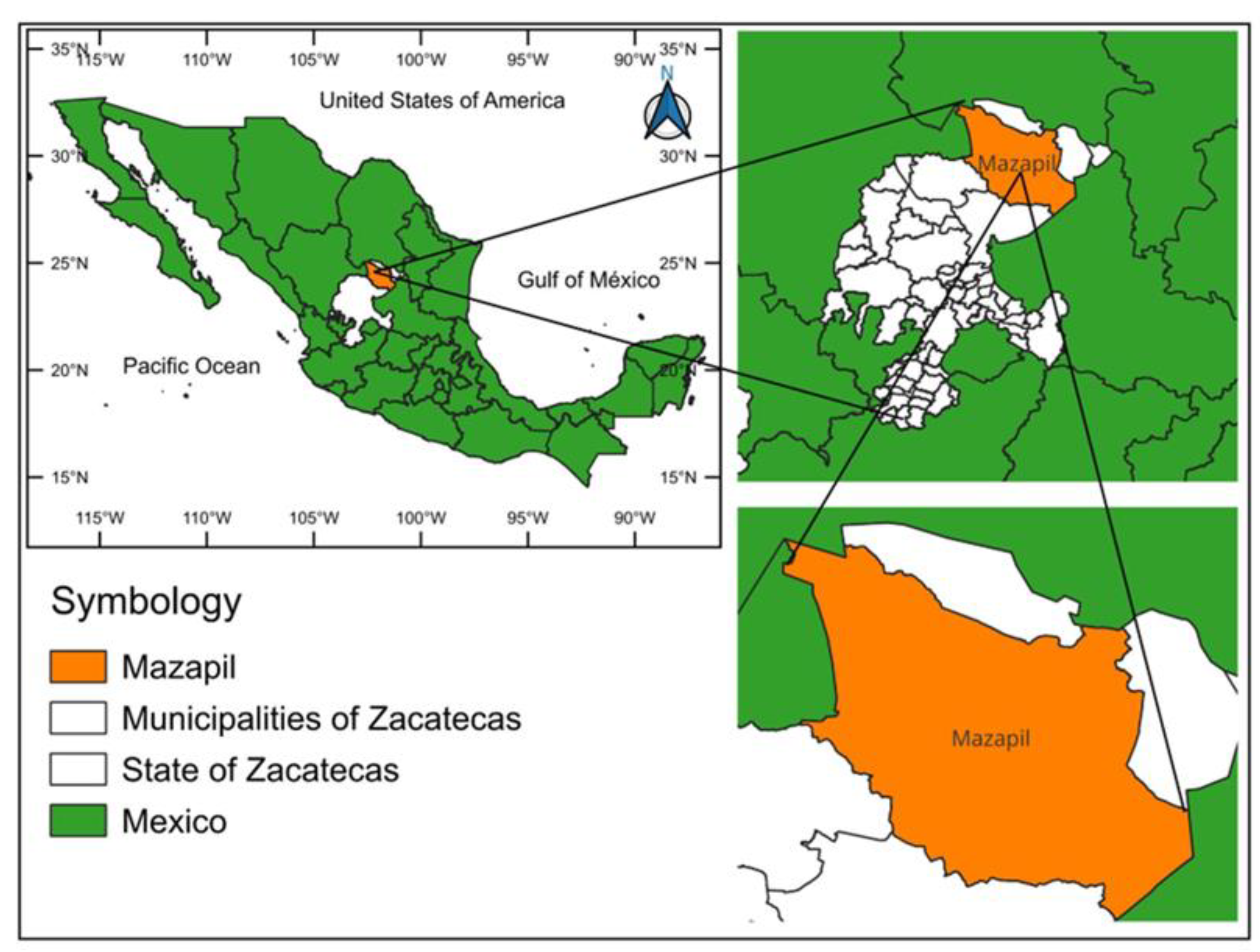
Figure 1.
a) Combination of bands B5 (SWIR 1), B4 (NIR), and B3 (Red) from Landsat 5 imagery gotten on 09/02/1998. b) Combination of bands B6 (SWIR 1), B5 (NIR), and B4 (Red) from Landsat 8 imagery gotten on 05/02/2014 [35].
Figure 1.
a) Combination of bands B5 (SWIR 1), B4 (NIR), and B3 (Red) from Landsat 5 imagery gotten on 09/02/1998. b) Combination of bands B6 (SWIR 1), B5 (NIR), and B4 (Red) from Landsat 8 imagery gotten on 05/02/2014 [35].
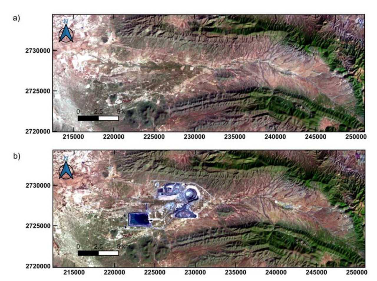
Figure 3.
(a) Landforms prior to mining activity derived from the 1998 INEGI DEM. (b) Landforms after mining activity generated from the 2014 Copernicus DEM.
Figure 3.
(a) Landforms prior to mining activity derived from the 1998 INEGI DEM. (b) Landforms after mining activity generated from the 2014 Copernicus DEM.
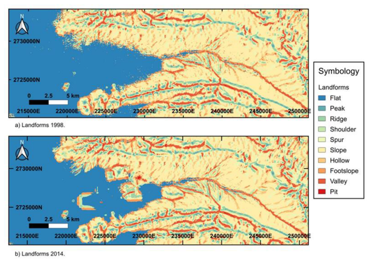
Figure 4.
Elevation differences between a) 2014 Copernicus DEM and the 1998 INEGI DEM, b) 2014 Copernicus DEM and the 1999 SRTM DEM, and c) 2014 Copernicus DEM and 2000 ASTER DEM.
Figure 4.
Elevation differences between a) 2014 Copernicus DEM and the 1998 INEGI DEM, b) 2014 Copernicus DEM and the 1999 SRTM DEM, and c) 2014 Copernicus DEM and 2000 ASTER DEM.
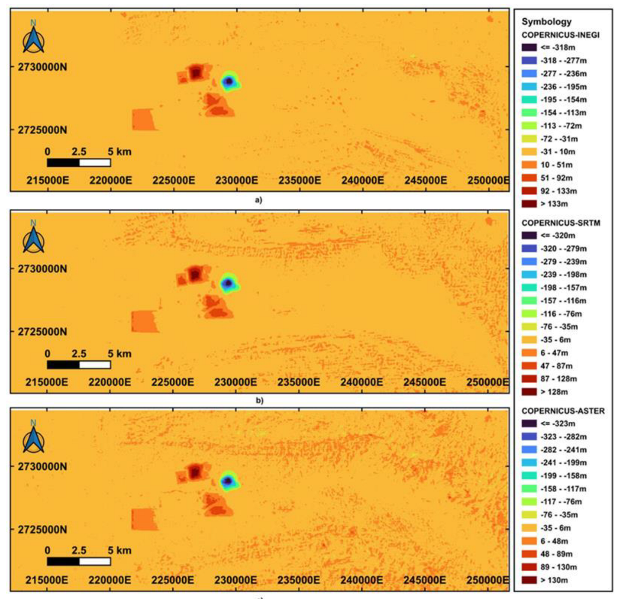
Figure 5.
Standard deviation map of the Copernicus–INEGI, Copernicus–ASTER, and Copernicus–SRTM DEM comparisons.
Figure 5.
Standard deviation map of the Copernicus–INEGI, Copernicus–ASTER, and Copernicus–SRTM DEM comparisons.
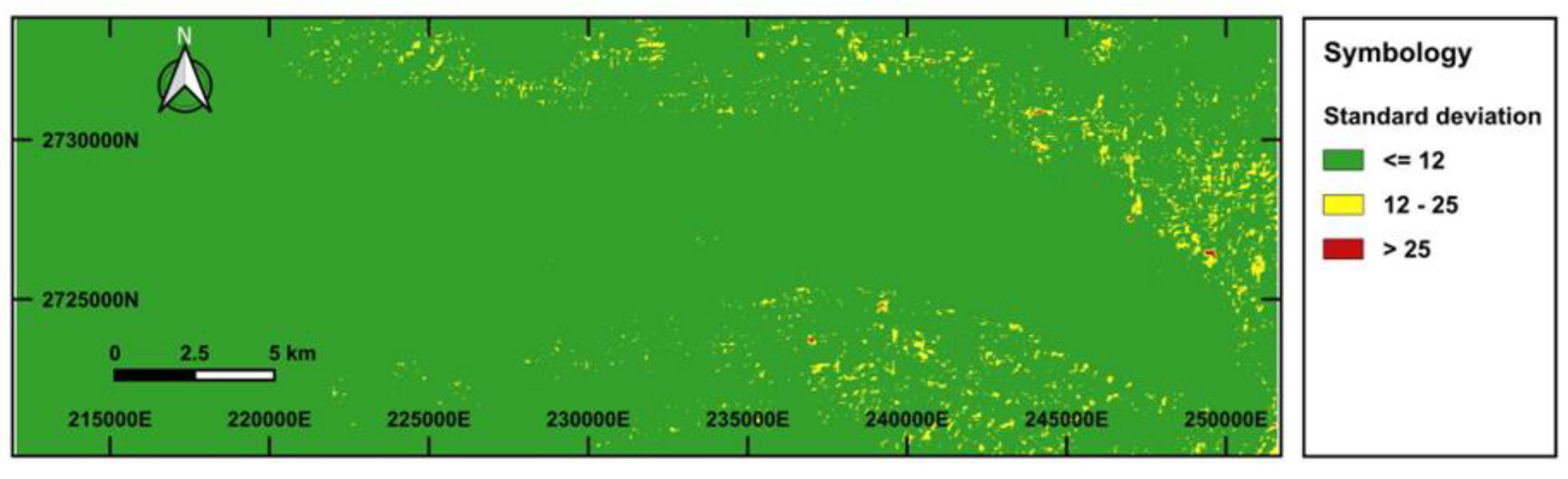
Figure 6.
Average elevation difference map derived from the Copernicus, INEGI, ASTER, and SRTM DEM.
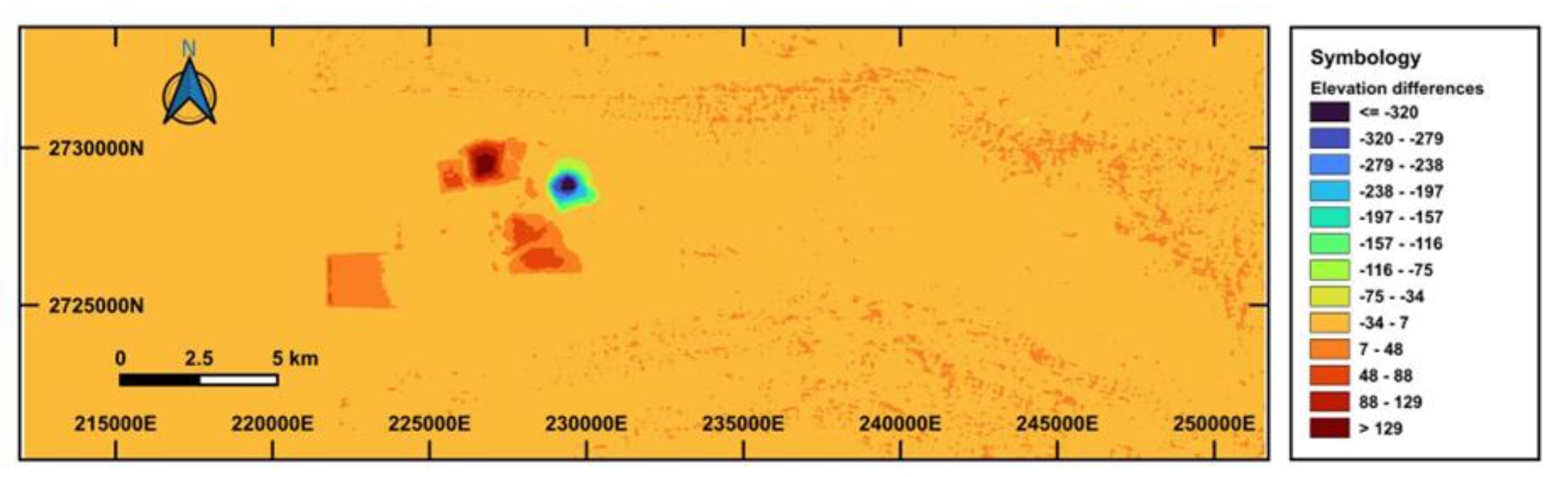
Figure 7.
Map of the mining area over Landsat 8 imagery from 2014.
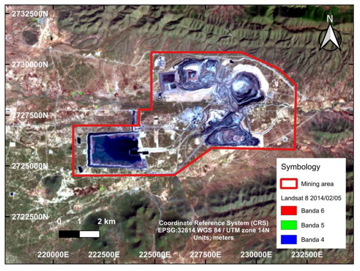
Figure 8.
Map of terrain alterations within the mining area.
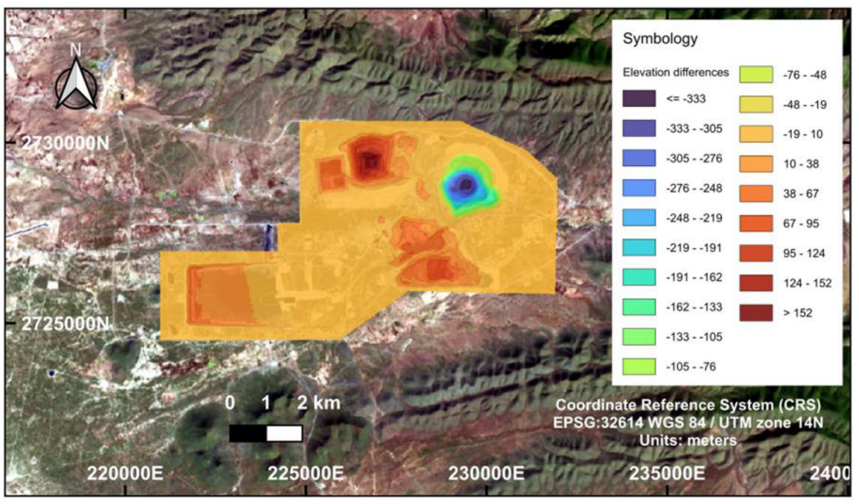
Figure 9.
Map of excavation and fill volumes within the mining area.
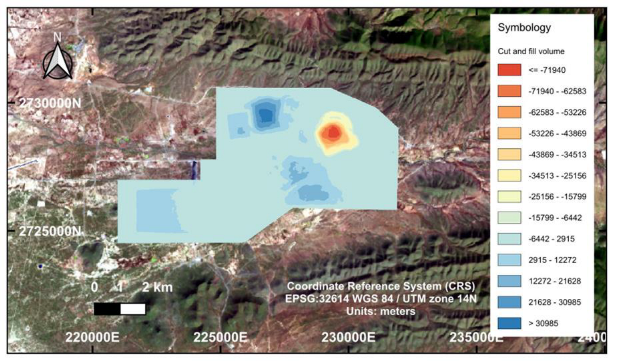

Table 1.
Mean vertical error, mean standard deviation, and mean square error for the ALOS, ASTER, and SRTM DEMs with the INEGI DEM.
Table 1.
Mean vertical error, mean standard deviation, and mean square error for the ALOS, ASTER, and SRTM DEMs with the INEGI DEM.
| Differences | ME (m) | SD (m) | RMSE (m) |
| ALOS-INEGI | -14.420 | 5.685 | 15.501 |
| ASTER-INEGI | 1.259 | 8.560 | 8.652 |
| SRTM-INEGI | 1.272 | 6.372 | 6.498 |
Table 2.
Mean vertical error, mean standard deviation, and mean square error for the ALOS, ASTER, and SRTM DEMs with the INEGI DEM.
Table 2.
Mean vertical error, mean standard deviation, and mean square error for the ALOS, ASTER, and SRTM DEMs with the INEGI DEM.
| Elevation range (m) | Area (km²) | Percentage (%) | Dominant feature |
| < -19 | 2.587 | 5.82% | Deep excavation |
| -19 to +10 | 29.281 | 65.8% | Areas of moderate and no alteration |
| > +10 | 12.632 | 28.38% | Waste or tailings deposit |
Table 3.
Volumetric calculation of excavation and fill within the mining footprint.
| Parameter | Volume |
| Excavation volume | 413,524,124 m³ |
| Fill volume | 431,194,785 m³ |
| Std. deviation per pixel | ±810 m³ |
| Max. excavation volume per pixel | −71,940 m³ |
| Max. fill volume per pixel | +30,985 m³ |
Disclaimer/Publisher’s Note: The statements, opinions and data contained in all publications are solely those of the individual author(s) and contributor(s) and not of MDPI and/or the editor(s). MDPI and/or the editor(s) disclaim responsibility for any injury to people or property resulting from any ideas, methods, instructions or products referred to in the content. |
© 2025 by the authors. Licensee MDPI, Basel, Switzerland. This article is an open access article distributed under the terms and conditions of the Creative Commons Attribution (CC BY) license (http://creativecommons.org/licenses/by/4.0/).
Copyright: This open access article is published under a Creative Commons CC BY 4.0 license, which permit the free download, distribution, and reuse, provided that the author and preprint are cited in any reuse.


