A Machine Learning Approach for Estimating Person Counts Using Anonymous WiFi Data in a University Library

1. Introduction

Smart campuses are emerging as a technological evolution of the smart city paradigm, driven by digital transformation and the integration of cyber-physical systems in higher education environments [1,2,3]. Within this framework, university libraries represent critical infrastructures where occupancy monitoring plays a central role in enabling dynamic space allocation, improving user experience, and supporting sustainable operations [4,5].

Indoor people monitoring operates basically at three hierarchical levels [6]: (1) presence, (2) people counting, and (3) individual identification. While presence detection and counting preserve anonymity, identification raises privacy concerns under regulations like the General Data Protection Regulation (GDPR) in the European Union, requiring strict compliance measures. Our work focuses on the counting level as it balances operational utility with privacy preservation.

Building occupancy monitoring systems employ diverse methodologies for person counting [7]: (1) environmental/presence sensors (e.g., CO₂, PIR), which are sensitive to ventilation and room typology, and therefore offer limited spatiotemporal resolution [8,9,10]; (2 computer vision, which can be highly accurate but entails higher deployment/maintenance costs and privacy risks [11,12]; and (3) wireless signals (Wi-Fi/BLE), which often provide the best trade-off between accuracy, cost, and anonymity.

Within wireless approaches, we distinguish two strategies: (1) passive detection (Wi-Fi probe requests, BLE advertisements), which does not require association but does require deploying sensors/probes and specialized hardware (thereby increasing implementation costs, especially at scale) [13], and (2) leveraging the existing Wi-Fi infrastructure, where APs act as soft sensors and provide more stable, persistent telemetry without installing additional sensors, reusing the already-deployed network and reducing deployment and maintenance costs. Nevertheless, Wi-Fi–infrastructure–based methods face key challenges: (1) the difficulty of obtaining reliable ground truth at scale in an automated and sustained manner over time; and (2) the prevalence of short temporal windows (weeks/months) in prior studies, which hinders capturing seasonal behaviors and assessing long-term viability and robustness against temporal drift.

In this work, we analyze the long-term viability of Wi-Fi telemetry for occupancy estimation. To this end, we build an eight-month labeled dataset (November 2024–June 2025) using a continuous, automated pipeline that integrates institutional Wi-Fi telemetry with a computer-vision system that provides automatic and reliable ground truth. The feature vector is enriched by distinguishing randomized vs. static MAC addresses to infer device class (mobile vs. laptop/desktop) in aggregate, while preserving anonymization and privacy compliance. Our primary goal is to evaluate the temporal robustness of the models (to detect potential performance degradation over time) and to validate their behavior when trained and tested across extended, heterogeneous conditions, confirming stable performance over the course of an academic term. Additionally, we conduct a systematic comparison of regression families (linear (Ridge), instance-based (KNN), margin-based (SVR), tree ensembles (Random Forest, ExtraTrees, XGBoost), and neural networks (MLP)) to determine which approaches are best suited to this task under a common training/validation protocol.

The rest of the paper is organized as follows. Section 2 surveys related work on Wi-Fi–based occupancy estimation and adjacent approaches. Section 3 describes the case study site. Section 4 details the dataset generation pipeline and feature engineering. Section 5 presents the training methodology. Section 6 reports the results, including comprehensive performance metrics and validation against ground-truth occupancy. Finally, Section 7 concludes and outlines directions for future work.

2. Related Work

One of the main obstacles in Wi-Fi–infrastructure–based occupancy estimation is obtaining large-scale labeled data, that is, reliable and continuous measurements of true occupancy (ground truth) for training and validating models. On-site manual counting is costly and unsustainable, which restricts studies to short temporal windows and exposes them to human error.

In response to this challenge, many studies have adopted calibration heuristics based on device-to-person conversion factors. Typically, during a short calibration period (one or two weeks), both headcounts and the number of connected devices per area are recorded; the average ratio is then used as a multiplier to estimate occupancy thereafter. For example,[14] estimated campus occupancy at the University of New South Wales by counting Wi-Fi devices over four weeks and applying a fixed factor of 1.3, achieving a correlation of r = 0.85 with observed occupancy. While pragmatic, this approach fails to capture real-world variability: the device-to-person ratio shifts with the academic calendar (exams, holidays), usage patterns, and other contextual factors.

In parallel, some authors have explored capture–recapture methods to infer the number of individuals from observed identifiers [15], with reported Mean Absolute Error (MAE), defined as the average absolute difference between estimated and actual values, ranging from 3 to 40 people depending on the occupancy level. However, applying this approach to Wi-Fi is constrained by MAC address randomization, which introduces time-varying identifiers and detection biases. These effects violate key assumptions of capture–recapture (e.g., persistent and independent “marks”), making consistent estimation difficult.

To mitigate the lack of labels, another line of work integrates computer vision as an automated source of ground truth. The most common systems use top-view cameras with line-based counting to tally entries and exits, synchronizing these data with Wi-Fi telemetry to train supervised models. In this vein, studies in offices with peaks of 48–74 people over 5 weeks categorize devices by connection time [16]; other work in classrooms (maximum capacity ≈80) with 1 week of data reports R² = 0,703 [17]; and 6-week studies in conference rooms (capacity ≈100) report R² = 0,958 [18]. Additionally, [19] presents models trained on 9 weeks of Wi-Fi logs from a Montreal university library (maximum capacity ≈2200), using variables such as number of MACs, day, and hour, achieving R² values between 0.92 and 0.96.

This hybridization reduces manual effort and improves labeling fidelity, yet most studies remain constrained to short periods (≈2–3 months). This limitation prevents observing seasonal phenomena (start of term, exam periods, holidays) and hinders a solid assessment of the model’s temporal robustness. In this regard, [4] shows that distinct occupancy patterns can be identified over a full academic year, underscoring the need for longer data series to ensure the validity of the estimates.

The main contributions of this work are as follows:

• Longitudinal evaluation: We conduct an eight-month study (November 2024–June 2025) spanning multiple seasonal regimes, providing a broader temporal scope than prior short-term evaluations.
• Methodological design: We leverage institutional Wi-Fi telemetry combined with a top-view, line-based computer vision counter as continuous ground truth, and enforce a strict non-overlapping split (four months for training, four months for testing) without intermediate retraining, to emulate real production conditions.
• Detailed performance analysis: Beyond reporting global metrics, we assess temporal robustness by tracking weekly MAE to detect performance drift and analyze errors by occupancy level, covering low, medium, and high loads.
• Comparative modeling study: We benchmark multiple regression families (including linear/margin-based, instance-based, tree ensembles, and neural models) to identify the most suitable approaches for the occupancy estimation problem.

3. Methodology and Case Study

The use case is Antigones Library, located in the building of the School of Telecommunications Engineering. It is the main library of the Universidad Politécnica de Cartagena (UPCT). The library is equipped with a top-view, line-based counting system at its main entrance, which provides an automated and continuous ground truth of occupancy with high accuracy. This setup enables sustained data generation over time and supports the supervised validation of occupancy-estimation models using logs from the existing Wi-Fi infrastructure.

3.1. Process Framework: CRISP-ML(Q)

We follow the CRISP-ML(Q) process model to structure the study and embed quality assurance [20]. The framework comprises business and data understanding, data engineering, model engineering, evaluation, deployment, and monitoring and maintenance. In this feasibility setting we instantiate the first four phases; deployment and monitoring are emulated offline (train once, evaluate on a four-month holdout, weekly MAE and drift checks). The subsequent sections cover each phase in context: Section 3.2, Section 3.3, Section 3.4 (understanding and data sources), Section 4 (data engineering), Section 5 (model engineering), and Section 6 (models’ evaluation).

3.2. Study Area

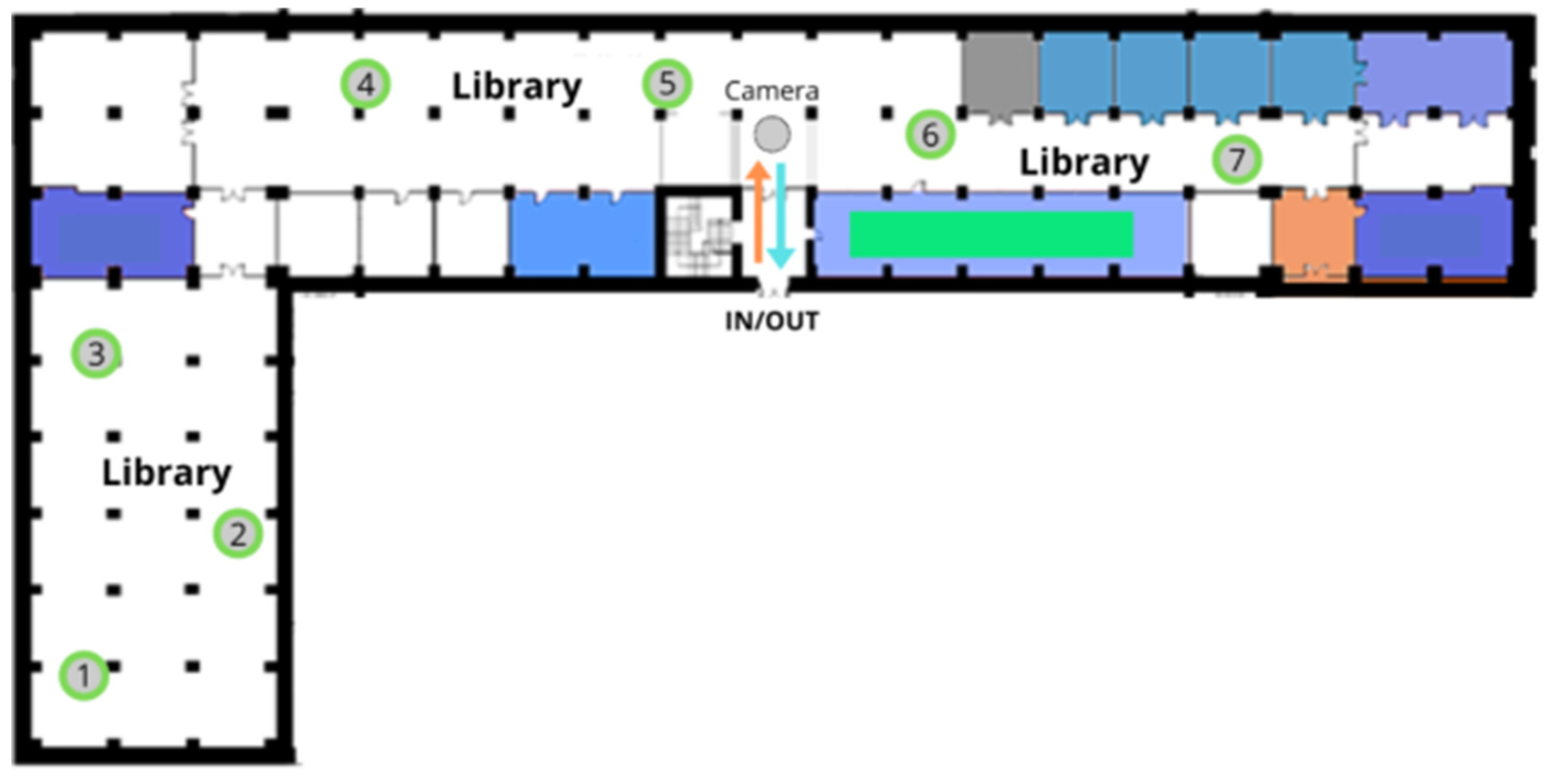
The library is a university venue of approximately 1.900 m², with a maximum capacity of 270 people. Inside the building, seven Wi-Fi access points (APs) are deployed; these APs act as soft sensors, providing counts and telemetry of the devices connected within the facility.

Operationally, the library is open Monday–Friday, 08:00–21:30 (closed on weekends). The analysis period spans November 2024 to June 2025, which yields observations across low (vacation), medium (regular term), and high (exam periods) occupancy regimes.

Assumptions for this environment:

• Seasonality and prolonged stays. As a study space, users typically remain for extended intervals, leading to relatively stable occupancy over time and persistent Wi-Fi sessions across sampling intervals.
• Multiple devices per user. A single user may carry 0, 1, 2, or more devices (e.g., smartphone, laptop, tablet). This non-one-to-one device person relationship adds complexity to occupancy estimation (the ultimate target), which we address through feature engineering and modeling.

3.3. Wi-Fi Infrastructure

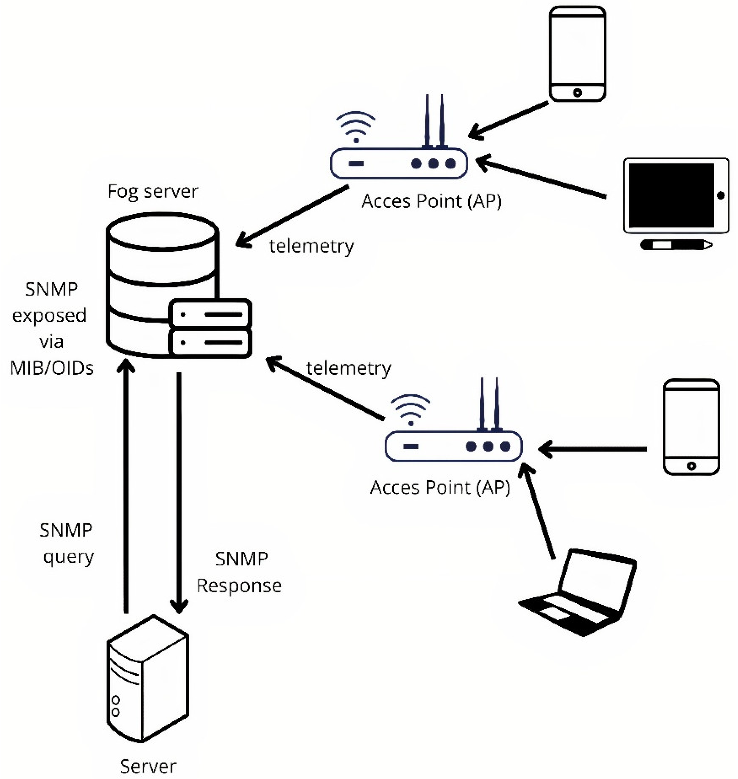
As shown in Figure 1, the library contains seven Wi-Fi access points (APs) distributed across the floor area. Beyond providing wireless coverage, these APs act as soft sensors: they record signals from associated devices that serve as proxies to estimate occupancy. All telemetry is centralized by a controller (hereafter, Fog Server), which stores the data reported by the APs and exposes it via SNMP through its MIB. Each metric is available as an object identified by an OID (Object Identifier). This design enables remote querying of the variables of interest without needing direct access to each individual AP.

Figure 2. Data flow in the Wi-Fi infrastructure.

Figure 2. Data flow in the Wi-Fi infrastructure.

3.4. Computer-Vision System

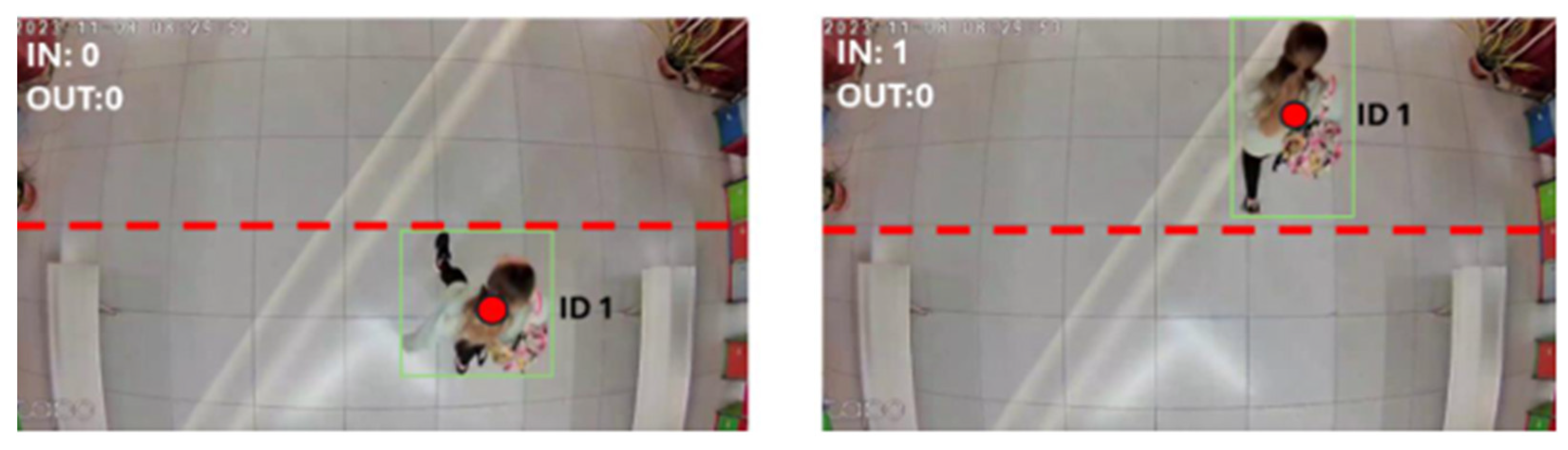
The library employs a line-based counting system installed in the entrance corridor. The method defines a virtual line on the top-view image and counts entries and exits according to the crossing direction. From these events, the system integrates the instantaneous occupancy of the room, producing an automated and continuous ground truth during operating hours.

The detector is based on a YOLO person detector coupled with a tracking algorithm, which preserves object identity while crossing the line. In internal validations, the system achieves >94% accuracy in counting entries and exits [21].

Figure 3. Example of automated entry/exit detection.

Figure 3. Example of automated entry/exit detection.

The system exposes a REST API that provides per-minute occupancy (timestamp and cumulative occupancy) for a given day, enabling automated ground-truth collection.

4. Dataset Generation

4.1. Features Selection

As part of the Exploratory Data Analysis (EDA), we audited 18 telemetry fields exposed by the Fog Server via SNMP and evaluated them under four criteria: (i) proxy relevance for occupancy, (ii) data quality, measured by missingness and temporal stability across access points and time slots, (iii) portability across sites, avoiding highly site-specific fields, and (iv) privacy compliance under GDPR.

We keep a minimal, high-quality set that serves as robust proxies while preserving privacy: (1) device MAC address, (2) associated AP IP, (3) bytes transmitted per device, (4) bytes received per device and (5) association uptime.

EDA indicated that several fields fail at least one criterion:

• Operating system type, more than 40% unknown and with unclear derivation, which undermines data quality and interpretability.
• User device IP adds no information beyond device counts inferred from MACs and increases privacy exposure.
• Human-readable names or labels, potentially identifying, therefore excluded for anonymization.
• Wlan ID and similar network configuration fields, too site dependent, low external validity.
• Redundant traffic transformations, alternative encodings of the same byte counters that add no new signal.
• Packet retry counters, noisy and driven by RF conditions rather than headcount, weak occupancy proxy in this setting.
• Constant or non-discriminative fields, for example link type wired versus Wi-Fi when all sessions are Wi-Fi.

Table 1. Selected Telemetry Features: Usage and Rationale.

Telemetry field (example)	Used	Rationale
Device MAC	Yes	Aggregate counts and randomized vs static split; raw MAC not modeled
Associated AP IP	Yes	AP-level aggregation and device–AP association
Bytes TX / Bytes RX	Yes	Direct activity proxies with low missingness
Association uptime	Yes	Session persistence proxy
OS type	No	>40% unknown; unclear derivation
Device IP	No	Redundant for counting; privacy exposure
Human-readable name/label	No	Privacy-sensitive
Wlan ID	No	Site-specific; low portability
Packet retries (TX/RX)	No	RF-driven noise; weak proxy
Alternative traffic formats	No	Redundant transformations

Table 1. Selected Telemetry Features: Usage and Rationale.

Telemetry field (example)	Used	Rationale
Device MAC	Yes	Aggregate counts and randomized vs static split; raw MAC not modeled
Associated AP IP	Yes	AP-level aggregation and device–AP association
Bytes TX / Bytes RX	Yes	Direct activity proxies with low missingness
Association uptime	Yes	Session persistence proxy
OS type	No	>40% unknown; unclear derivation
Device IP	No	Redundant for counting; privacy exposure
Human-readable name/label	No	Privacy-sensitive
Wlan ID	No	Site-specific; low portability
Packet retries (TX/RX)	No	RF-driven noise; weak proxy
Alternative traffic formats	No	Redundant transformations

4.2. Feature Engineering

To make the collected information useful for predictive modeling, we apply a transformation and enrichment process. In particular, the MAC addresses exposed by the controller allow us to infer indirect information about the device type. To this end, each MAC is classified into one of two mutually exclusive categories:

• Randomized MACs: addresses generated dynamically by the operating system to preserve privacy. These addresses change frequently and are identified because the second hexadecimal digit of the first byte takes the value 2, 6, A, or E (i.e., the locally administered bit is set).
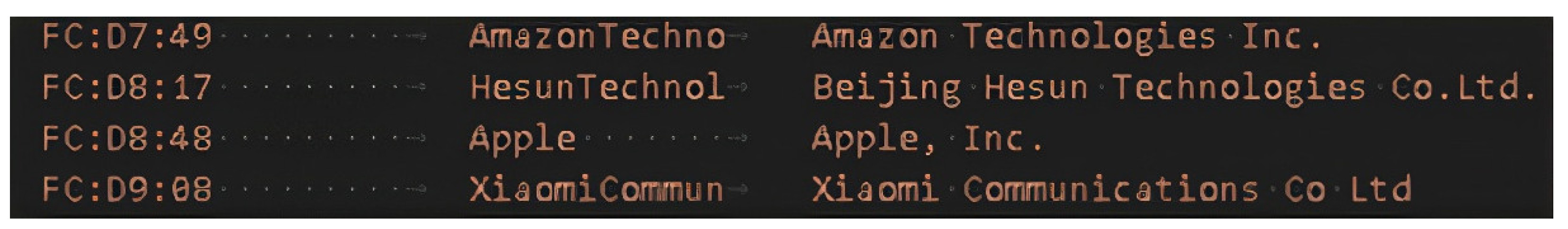
• Static MACs: globally unique addresses assigned by the manufacturer that retain a valid OUI (Organizationally Unique Identifier). Classification is performed by matching the first three bytes against a manufacturer database (e.g., the Wireshark Manufacturer Database).

Figure 4. Extract from the Wireshark Manufacturer Database.

Figure 4. Extract from the Wireshark Manufacturer Database.

4.3. Data Pipeline Architecture: Wi-Fi Ingestion and Feature-Vector Construction

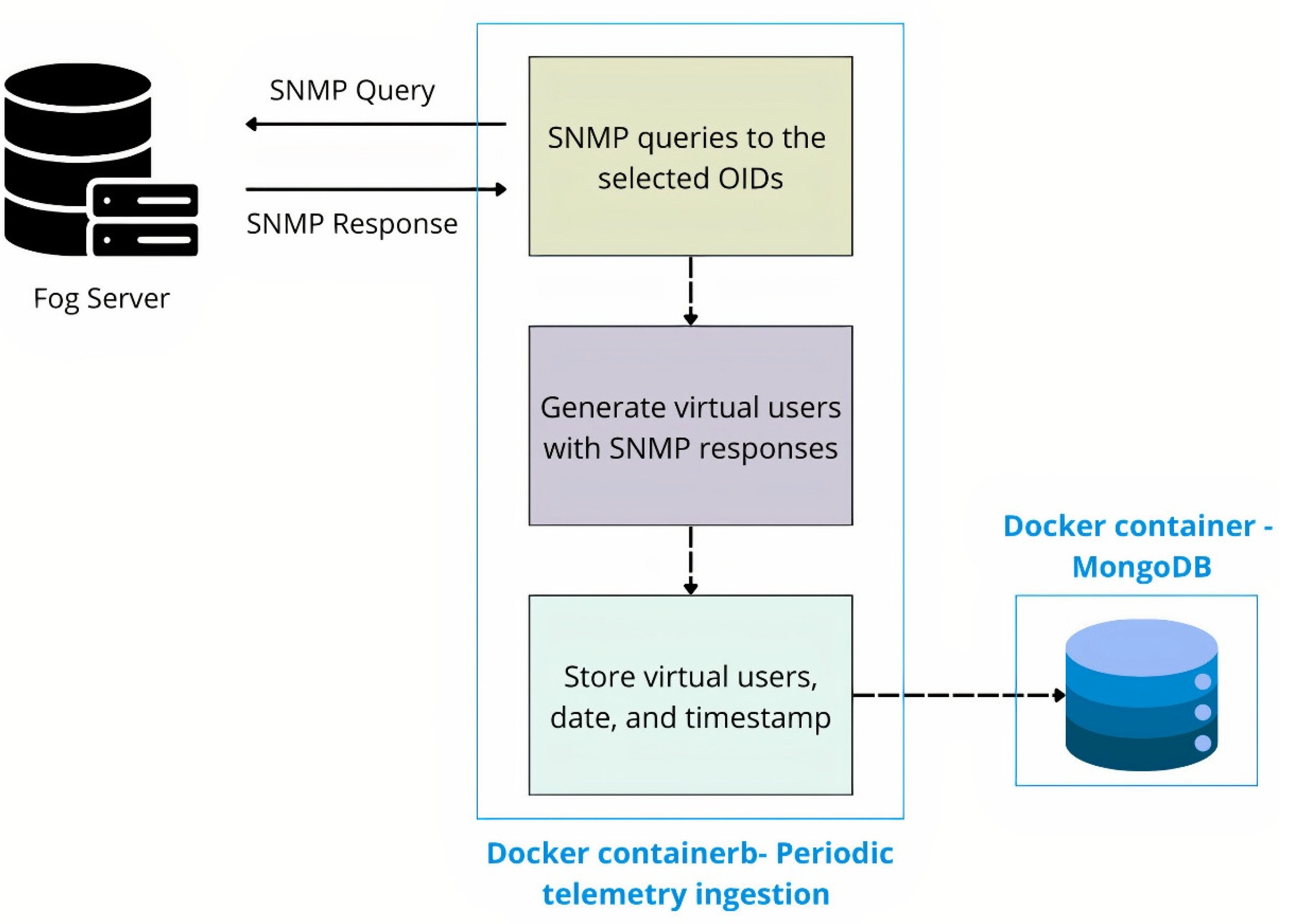
4.3.1. Module I — Periodic Telemetry Ingestion (Historical)

This module issues periodic SNMP queries to the Fog Server to build a history of associated devices and the selected variables. In each cycle, the defined OIDs are queried, and the telemetry is consolidated by linking all variables for the same device (MAC, AP IP, transmitted bytes, received bytes, and association uptime) to obtain a unified per-device view at each interval. The resulting snapshot is stored in the database with its timestamp. A 3-minute cadence is used to complete queries and writes without overlapping, ensuring regular sampling over time.

Figure 5. Periodic telemetry ingestion pipeline.

Figure 5. Periodic telemetry ingestion pipeline.

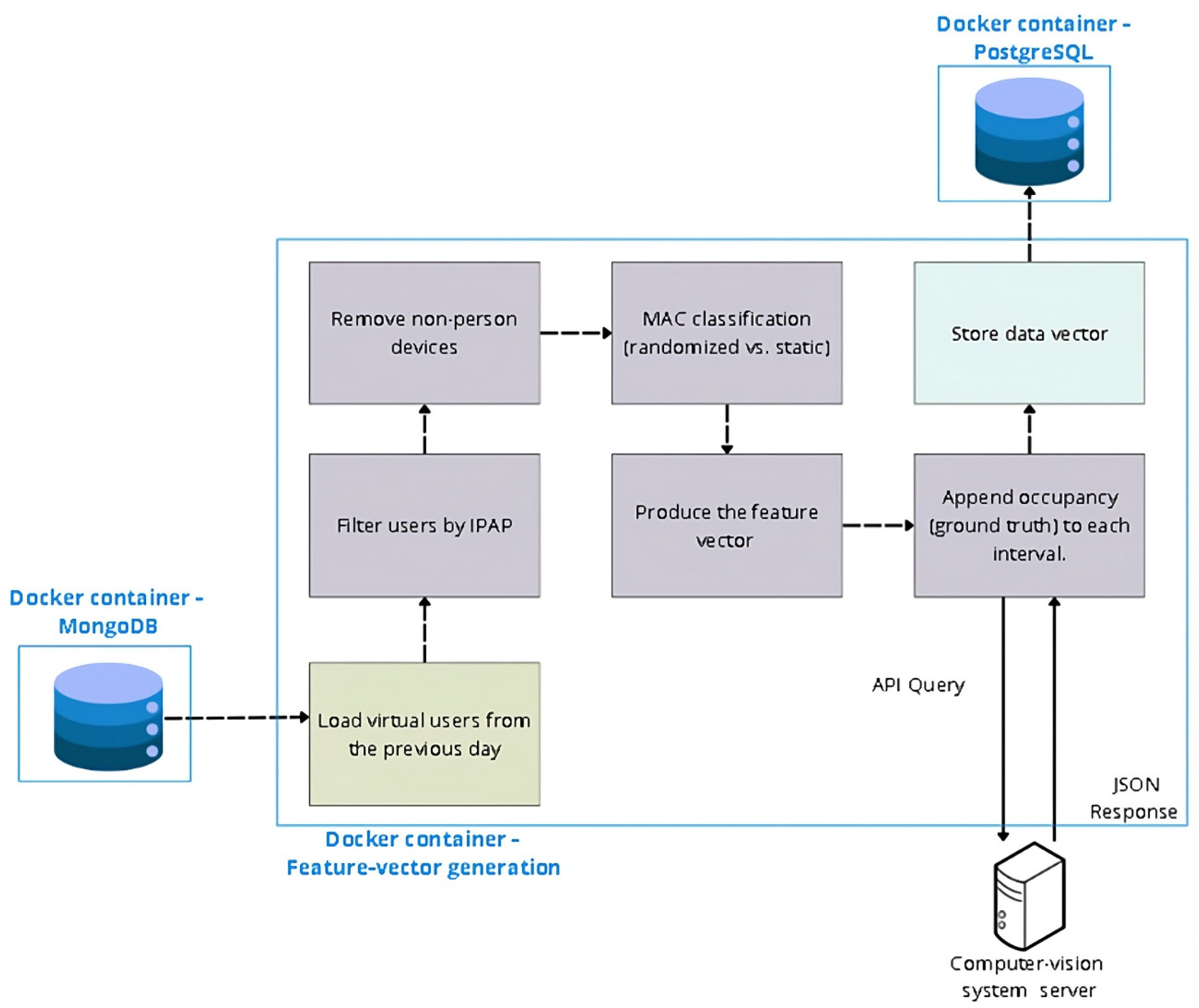
4.3.2. Module II — Feature-Vector Generation

Once per day, using the previous day’s history, we generate the data (feature) vector that describes the library’s state at each 3-minute timestamp. First, all ingestion records from the previous day are loaded; then they are filtered by AP to restrict the scope to the study area. Next, non-person devices are pruned, removing activity outside opening hours (overnight presence). On the resulting set we apply feature engineering, including MAC classification (randomized vs. static), and produce the feature vector for each time interval. Finally, the REST API of the computer-vision system is queried to append the corresponding occupancy (ground truth) to each interval.

Figure 1. Feature-vector generation pipeline.

Figure 1. Feature-vector generation pipeline.

4.4. Feature Vector

The pipeline in Section 4.3.2 produces a structured, consistent, and representative dataset to feed occupancy-prediction models on campus spaces. Each row captures the aggregate state of the study area at a 3-minute timestamp, combining features derived from Wi-Fi telemetry with the target variable (ground-truth occupancy from the vision system).

Table 2. Feature vector.

Variable	Type	Description
day_of_week	Categorical	Day of week (1 = Monday, …, 7 = Sunday).
timeslot_id	Categorical	Numeric ID of the 3-minute time slot within the day (e.g., 0: 08:00; 1: 08:03; …).
devices_total	Numeric	Total number of unique devices detected.
devices_randomized_mac	Numeric	Number of devices with randomized MAC.
devices_static_mac	Numeric	Number of devices with static MAC (valid OUI).
devices_persisting	Numeric	Devices present in both the previous and current interval (t−1 and t).
devices_new	Numeric	Devices present in t but not in t−1.
bytes_tx	Numeric	Bytes transmitted during the interval.
bytes_rx	Numeric	Bytes received during the interval.
bytes_total	Numeric	Sum of transmitted and received bytes.

Table 2. Feature vector.

Variable	Type	Description
day_of_week	Categorical	Day of week (1 = Monday, …, 7 = Sunday).
timeslot_id	Categorical	Numeric ID of the 3-minute time slot within the day (e.g., 0: 08:00; 1: 08:03; …).
devices_total	Numeric	Total number of unique devices detected.
devices_randomized_mac	Numeric	Number of devices with randomized MAC.
devices_static_mac	Numeric	Number of devices with static MAC (valid OUI).
devices_persisting	Numeric	Devices present in both the previous and current interval (t−1 and t).
devices_new	Numeric	Devices present in t but not in t−1.
bytes_tx	Numeric	Bytes transmitted during the interval.
bytes_rx	Numeric	Bytes received during the interval.
bytes_total	Numeric	Sum of transmitted and received bytes.

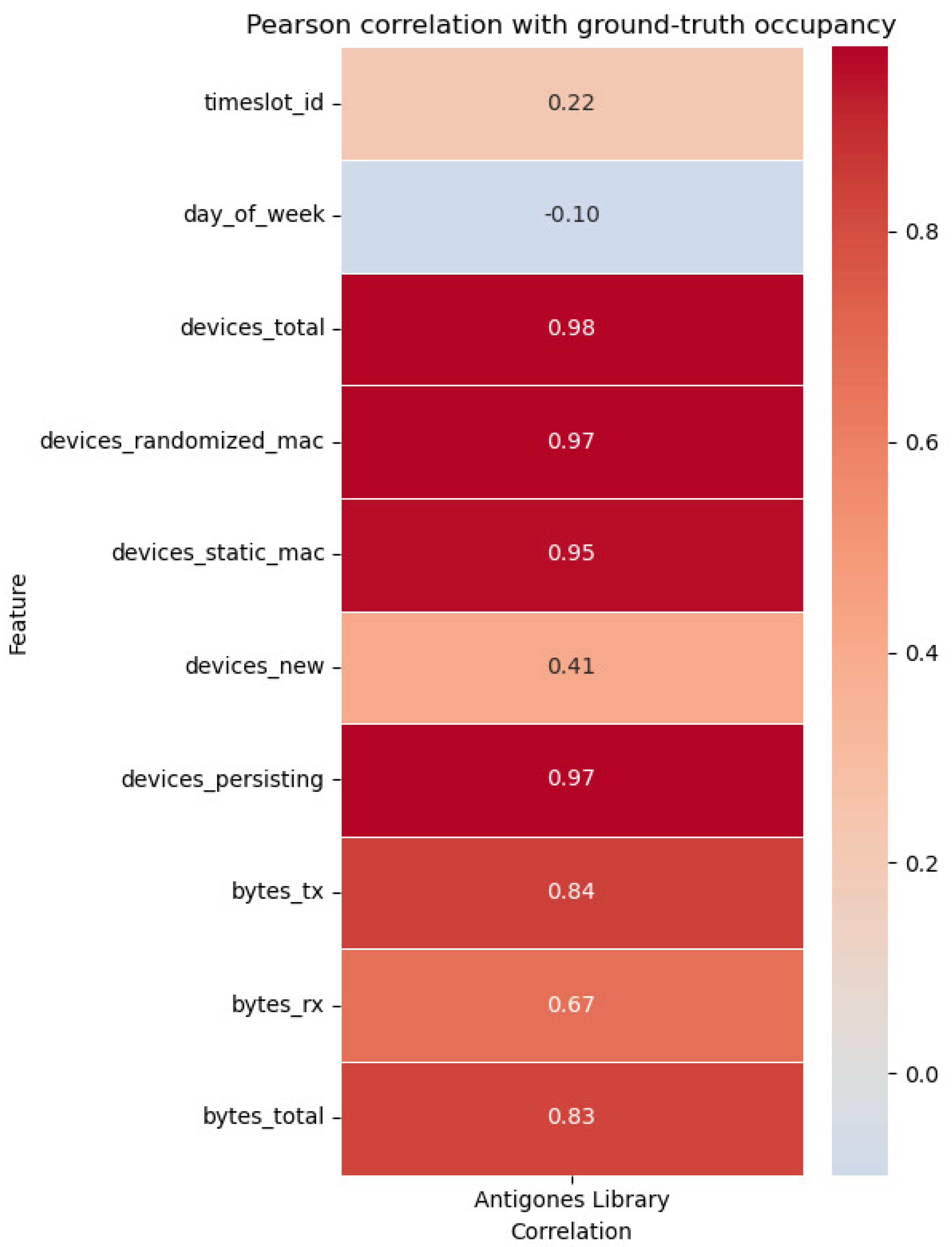
To further assess the representativeness of the feature vector, we computed Pearson correlations between each candidate feature and the ground-truth occupancy. As shown in Figure 7, device-based features exhibit the highest correlation values (≈0.95–0.98), while traffic-based variables (bytes transmitted/received) also correlate positively (≈0.67–0.84).

Figure 7. Pearson Correlation of Telemetry Features with Ground-Truth Occupancy.

Figure 7. Pearson Correlation of Telemetry Features with Ground-Truth Occupancy.

4.5. Temporal Scope of the Dataset

The dataset was built from eight months of data (November to late June) and split into two nonoverlapping temporal blocks to ensure diversity and robustness:

• Training set: 86 days from November 2024 to February 2025, used to train the models.
• Test set: 91 days from March 2025 to June 2025, used to simulate production conditions without intermediate retraining.

Both periods include heterogeneous usage scenarios (low-activity days, typical term days, and exam-period peaks) allowing performance to be assessed across varied contexts and reducing bias tied to specific days or situations. Days when the vision system’s cameras were inoperative were excluded, as the ground-truth occupancy label could not be guaranteed.

5. Training Methodology

This study evaluates seven algorithms spanning complementary families: a linear model (Ridge), an instance-based method (KNeighborsRegressor), a margin-based model (Support Vector Regression, SVR), three tree ensembles (RandomForestRegressor, ExtraTreesRegressor, XGBRegressor), and a multilayer perceptron (MLP). This selection contrasts different inductive biases to identify which approach best fits occupancy estimation from Wi-Fi telemetry.

Preprocessing was identical across models and implemented with pipelines to prevent data leakage. The categorical variables day_of_week and timeslot_id were encoded via one-hot encoding, while the continuous variables bytes_tx and bytes_rx were standardized (zero mean, unit variance) to stabilize scale-sensitive algorithms such as KNN, SVR, and MLP. All transformations were fitted only on the training folds and then applied to their corresponding validation folds.

Training used 86 days of data spanning November 2024 to February 2025. For each algorithm, we performed hyperparameter optimization with Optuna, using stratified 5-fold cross-validation. In this context, the stratification variable was timeslot_id, which groups samples by their timestamp. Stratification ensures that each fold contains a representative distribution of these time slots, so that training and validation sets reflect similar temporal patterns. This is important because occupancy strongly depends on the time of day (e.g., morning vs. evening), and a naive split could lead to hour-of-day bias, where the model is trained predominantly on one set of hours but evaluated on another, artificially inflating or deflating performance. By preserving the temporal distribution of time slots across folds, we obtain a fairer assessment of model generalization.

The objective function was the Root Mean Squared Error (RMSE), defined as the square root of the average of squared differences between predicted and actual values, which penalizes larger errors more heavily than MAE. The mean RMSE across folds was minimized to select the best hyperparameters for each model, after which the final version was retrained on the full training set.

Table 3. Hyperparameter Search Space for Each Mode.

Model	Hyperparameter	Search type / range
SVR	C	Float in [1e−4, 1]
	epsilon	Float in [1e−5, 5]
	kernel	Categorical: linear, poly, rbf}
Ridge	alpha	Float in [1e−4, 1]
Random Forest	n_estimators	Integer in [10, 50]
	max_depth	Integer in [5, 30]
XGBoost	n_estimators	Integer in [3, 25]
	max_depth	Integer in [2, 30]
	learning_rate	Float in [0.01, 0.1]
	subsample	Float in [0.2, 0.6]
	colsample_bytree	Float in [0.5, 1.0]
Extra Trees	n_estimators	Integer in [10, 100]
	max_depth	Integer in [5, 30]
	min_samples_split	Integer in [2, 10]
	min_samples_leaf	Integer in [1, 5]
KNN	n_neighbors	Integer in [3, 30]
	weights	Categorical: uniform, distance}

Table 3. Hyperparameter Search Space for Each Mode.

Model	Hyperparameter	Search type / range
SVR	C	Float in [1e−4, 1]
	epsilon	Float in [1e−5, 5]
	kernel	Categorical: linear, poly, rbf}
Ridge	alpha	Float in [1e−4, 1]
Random Forest	n_estimators	Integer in [10, 50]
	max_depth	Integer in [5, 30]
XGBoost	n_estimators	Integer in [3, 25]
	max_depth	Integer in [2, 30]
	learning_rate	Float in [0.01, 0.1]
	subsample	Float in [0.2, 0.6]
	colsample_bytree	Float in [0.5, 1.0]
Extra Trees	n_estimators	Integer in [10, 100]
	max_depth	Integer in [5, 30]
	min_samples_split	Integer in [2, 10]
	min_samples_leaf	Integer in [1, 5]
KNN	n_neighbors	Integer in [3, 30]
	weights	Categorical: uniform, distance}

6. Results

After training the models with four months of data (November 2024–February 2025), we evaluated their performance on an independent 91-day test set (March–June 2025) covering low, medium, and high occupancy regimes.

6.1. Metrics (Mar–Jun 2025)

For each model we report metrics over the four test months:

• MAE (Mean Absolute Error): average error in number of people; indicates how many people, on average, the predictions deviate from the true occupancy.
• RMSE (Root Mean Squared Error): also an average error measure but penalizes large errors more strongly, making it sensitive to peaks/outliers.
• SMAPE (Symmetric Mean Absolute Percentage Error): a variation of the Mean Absolute Percentage Error (MAPE), which computes the average percentage difference between predicted and actual values. While MAPE is widely used due to its interpretability, it becomes unstable when actual values are close to zero. SMAPE addresses this issue by symmetrizing the denominator, making it more robust for low or near-zero occupancies and therefore more suitable for occupancy estimation.
• R² (coefficient of determination): fraction of the variance of true occupancy explained by the model relative to a baseline that predicts the test-set mean. In our context, we interpret R² as the model’s ability to track day-to-day rises and falls in occupancy. A high R² indicates good tracking of the temporal shape; R² ≈ 0 suggests no improvement over the mean; a indicates performance worse than that baseline.

Overall, the models achieve competitive metrics over an extended validation horizon. SVR delivers the best overall performance (lowest RMSE/MAE and the lowest SMAPE, with R² = 0.955). Ridge and MLP are very close, also with high R² ≈ 0.95. KNN, Random Forest, and Extra Trees form a second tier with similar results. XGBoost lags behind in this setting (higher RMSE and MAE, R² = 0.907). In sum, linear/margin-based approaches and MLP tend to perform slightly better, whereas tree ensembles show somewhat lower performance on this dataset.

Table 4. Performance Comparison of Models on the Test Set.

Model	RMSE	MAE	SMAPE	R2
Ridge	10.367	8.068	19.34	0.953
KNN	11.451	8.781	18.96	0.943
SVR	10.178	7.775	15.29	0.955
Random Forest	11.181	8.645	18.36	0.946
Extra Trees	11.393	8.790	18.85	0.944
XGBoost	14.696	10.508	19.21	0.907
MLP	10.64	8.40	19.98	0.95

Table 4. Performance Comparison of Models on the Test Set.

Model	RMSE	MAE	SMAPE	R2
Ridge	10.367	8.068	19.34	0.953
KNN	11.451	8.781	18.96	0.943
SVR	10.178	7.775	15.29	0.955
Random Forest	11.181	8.645	18.36	0.946
Extra Trees	11.393	8.790	18.85	0.944
XGBoost	14.696	10.508	19.21	0.907
MLP	10.64	8.40	19.98	0.95

6.2. Error by Occupancy Range

Figure 8 reports the Mean Absolute Error (MAE) across occupancy ranges, grouped in 20-person bins (from 0–20 up to 240–260). As expected, the absolute error increases with the number of users in the room, since prediction deviations naturally accumulate at higher occupancies. Three distinct patterns can be observed:

• XGBoost shows the steepest error growth. This behavior may be related to its strong sensitivity to hyperparameter tuning; the chosen configuration may not be optimal for this dataset, or the model may overfit medium ranges and generalize poorly in the extremes.
• ExtraTrees, KNN, and Random Forest (tree-based families) perform comparably well at low and medium ranges but deteriorate noticeably at high occupancies. This is likely explained by the scarcity of training samples in those ranges: high occupancy situations are less frequent and occur only on specific peak days.
• SVR, Ridge, and MLP achieve the most robust performance at high occupancies. Their linear (or margin-based) components allow them to extrapolate more gracefully when training data is sparse, making them less dependent on having many examples of extreme scenarios.

Figure 8. Mean Absolute Error (MAE) by occupancy interval.

Figure 8. Mean Absolute Error (MAE) by occupancy interval.

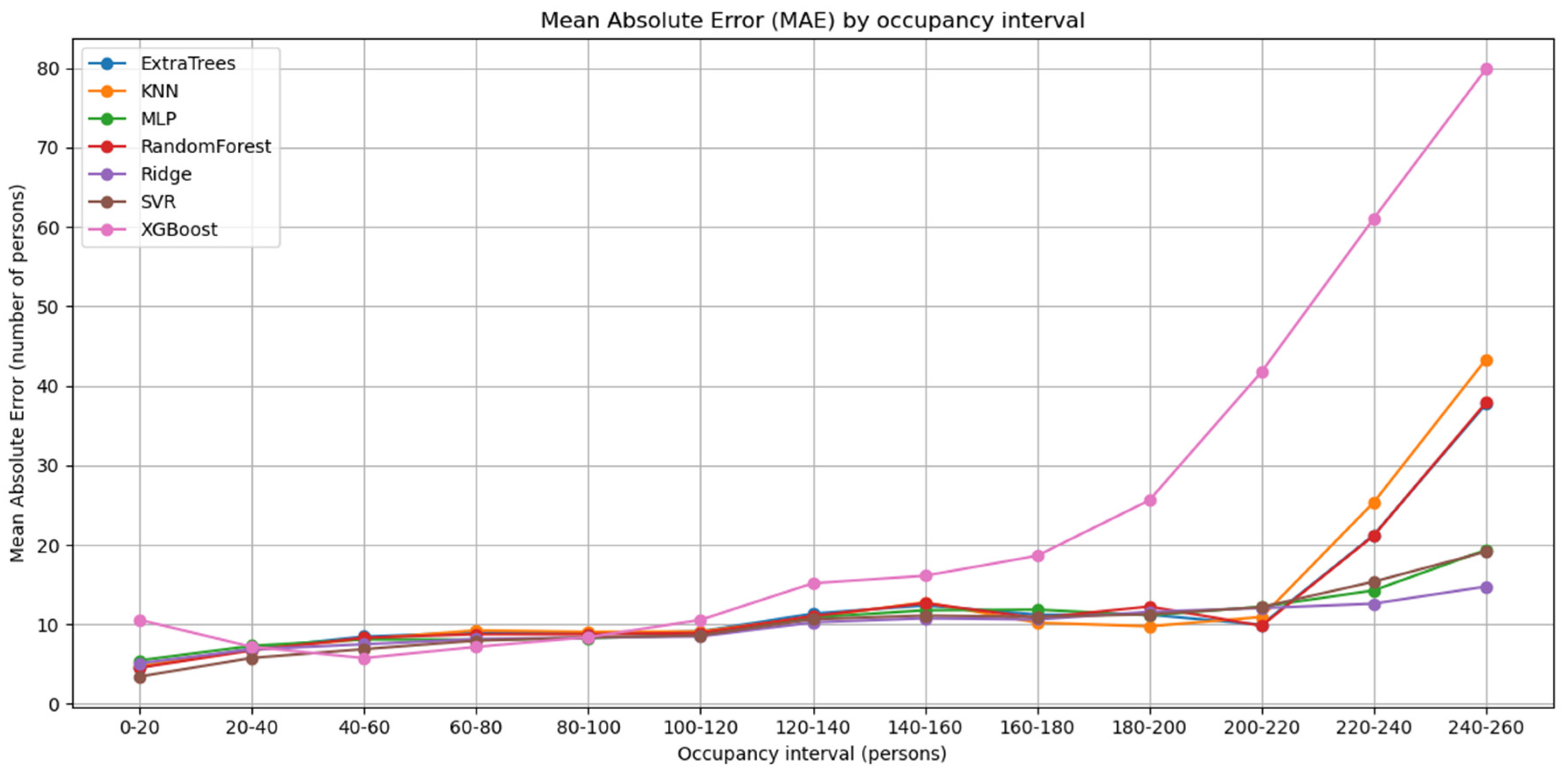
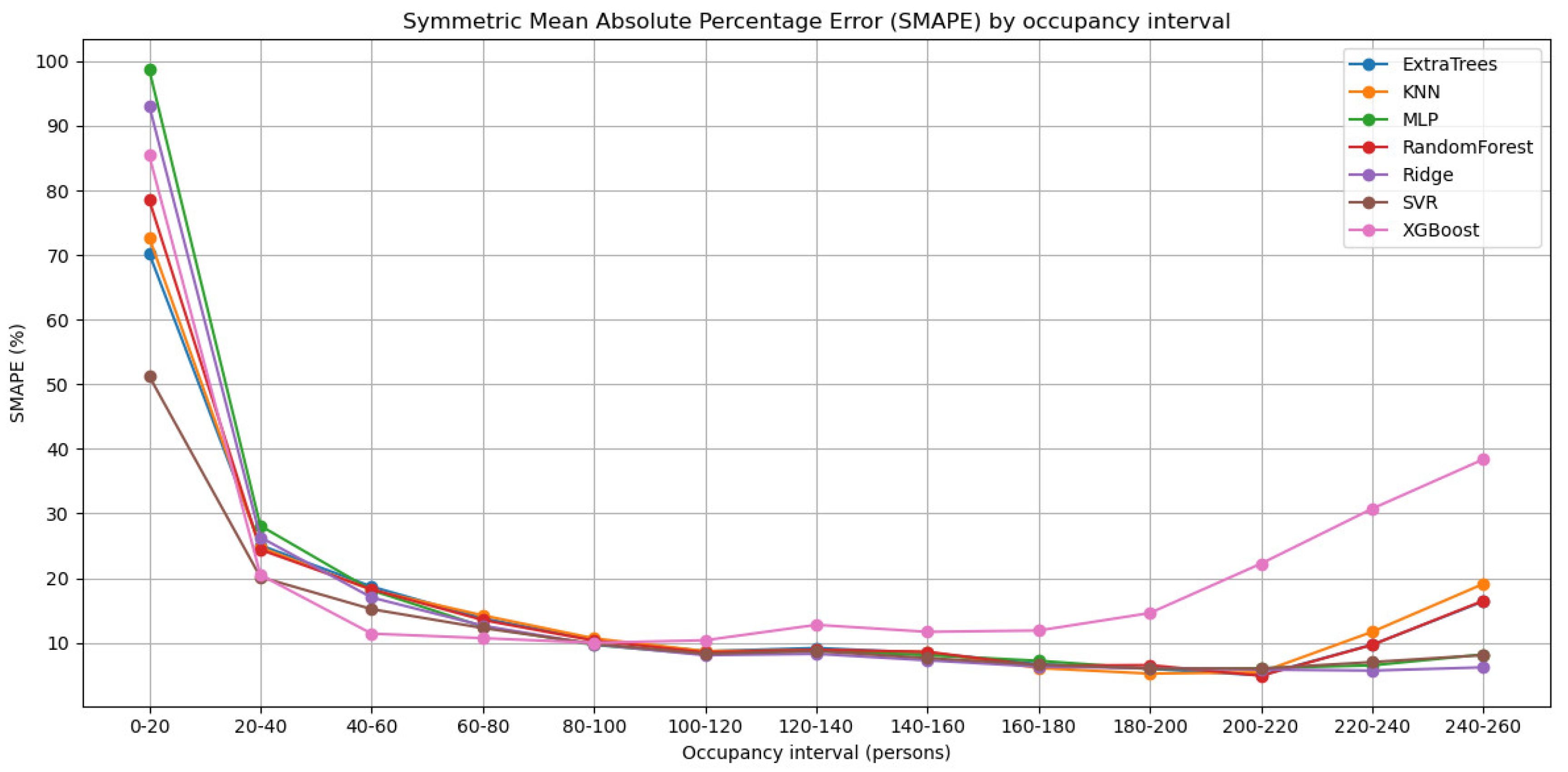
Figure 9 shows the Symmetric Mean Absolute Percentage Error (SMAPE) for the same occupancy ranges. Again, the three model families emerge. At very low occupancies, the relative error is high, in some cases approaching 100%. This is due to the variability in the device–person ratio: with only a few people in the room, a single individual carrying multiple devices (or none at all) can heavily distort the signal. Nevertheless, SVR already achieves relatively lower SMAPE values (≈50%), compared to 70–100% for the other models. As occupancy increases beyond ≈40 persons, the relative error rapidly stabilizes around 10% or lower for SVR, Ridge, and MLP, while tree-based ensembles degrade, and XGBoost shows the poorest behavior at the upper extremes. Overall, the analysis highlights that linear/margin-based models and MLP are more resilient to data scarcity at high occupancy, whereas tree ensembles are more dependent on sufficient training samples and prone to error amplification in rare extreme cases.

Figure 9. Symmetric Mean Absolute Percentage Error (SMAPE) by occupancy interval.

Figure 9. Symmetric Mean Absolute Percentage Error (SMAPE) by occupancy interval.

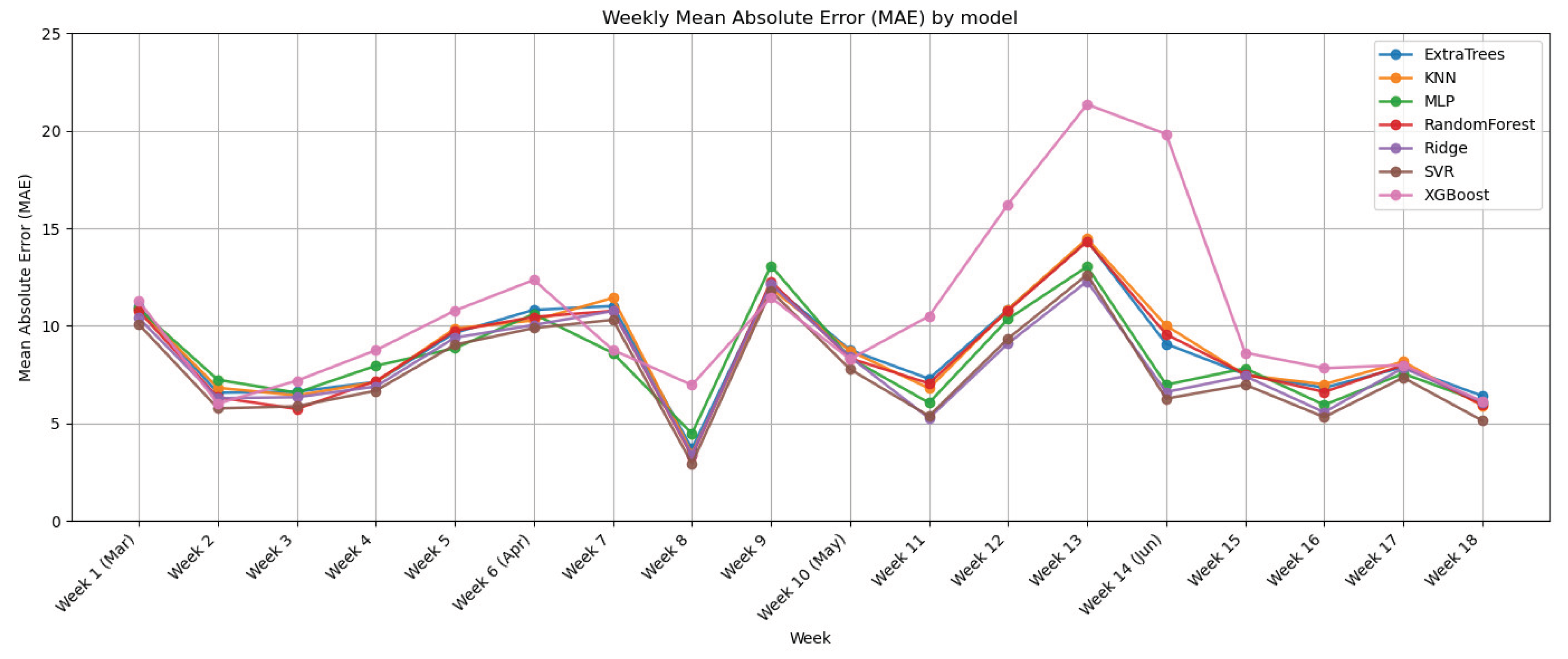
6.3. Temporal Stability (Weekly MAE)

To assess whether the models degrade over time (whether performance worsens as we move away from the training period), we aggregate errors by calendar week and plot the weekly MAE across the four test months. This aggregation reduces day-to-day noise and makes trends easier to spot. As shown in Figure X, there is no upward trend: the error remains around 8–10 people on average, with isolated peaks linked to specific situations. Consequently, we find no evidence of systematic degradation during March–June. Consistent with previous analyses, SVR, Ridge, and MLP achieve the lowest and most stable weekly MAE, while XGBoost stands out as the least robust, particularly in weeks with higher occupancy.

Figure 2. Weekly trend of mean absolute error (MAE).

Figure 2. Weekly trend of mean absolute error (MAE).

7. Discussion

This study presented a comparison of machine learning models for occupancy estimation from Wi-Fi telemetry, supported by an end-to-end automated pipeline that produced eight months of labeled data. The infrastructure enabled training on four months (Nov–Feb) and validation on an additional four months (Mar–Jun), thus significantly extending the evaluation horizon relative to prior work.

The results confirm competitive performance on the test set. As expected, absolute error (MAE) increases with occupancy, while relative error (SMAPE) stabilizes at around 10% for medium and high ranges. The main challenge appears at low occupancies, where the small number of people combined with the variable number of devices per person (from none to several) introduces high variability, making percentage-based metrics less reliable in these conditions.

Across model families, Ridge, SVR, and MLP consistently achieve the best performance, maintaining robustness across all occupancy levels. Their linear or margin-based nature allows them to extrapolate more effectively in rarely observed scenarios such as high-occupancy peaks, where tree ensembles (Random Forest, ExtraTrees, XGBoost) tend to degrade. Importantly, no temporal degradation was observed during the four-month validation period: MAE fluctuations reflected week-to-week variations in library usage (low vs. high occupancy days) rather than a systematic decline in model accuracy.

As future work, we plan to extend the validation horizon to longer periods (ideally a full year) to further confirm stability, evaluate the approach in additional buildings with different capacity ranges (including smaller venues where SMAPE challenges are most pronounced) and investigate prediction intervals to strengthen operational decision-making.

References

- Shihao, L.; Dahnil, D.P.; Saad, S. A Survey of Smart Campus Resource Information Management in Internet of Things. IEEE Access 2025, 13, 66622–66645. [Google Scholar] [CrossRef]
- Haggag, M.; Oulefki, A.; Amira, A.; Kurugollu, F.; Mushtaha, E.S.; Soudan, B.; Hamad, K.; Foufou, S. Integrating Advanced Technologies for Sustainable Smart Campus Development: A Comprehensive Survey of Recent Studies. Advanced Engineering Informatics 2025, 66, 103412. [Google Scholar] [CrossRef]
- Polin, K.; Yigitcanlar, T.; Limb, M.; Washington, T. The Making of Smart Campus: A Review and Conceptual Framework. Buildings 2023, 13, 891. [Google Scholar] [CrossRef]
- Alfalah, B.; Shahrestani, M.; Shao, L. Identifying Occupancy Patterns and Profiles in Higher Education Institution Buildings with High Occupancy Density – A Case Study. Intelligent Buildings International 2023, 15, 45–61. [Google Scholar] [CrossRef]
- Wang, Q.; Patel, H.; Shao, L. A Longitudinal Study of the Occupancy Patterns of a University Library Building Using Thermal Imaging Analysis. Intelligent Buildings International 2023, 15, 62–77. [Google Scholar] [CrossRef]
- Azimi, S.; O’Brien, W. Fit-for-Purpose: Measuring Occupancy to Support Commercial Building Operations: A Review. Building and Environment 2022, 212, 108767. [Google Scholar] [CrossRef]
- Chen, Z.; Jiang, C.; Xie, L. Building Occupancy Estimation and Detection: A Review. Energy and Buildings 2018, 169, 260–270. [Google Scholar] [CrossRef]
- Khan, I.; Cicirelli, F.; Greco, E.; Guerrieri, A.; Mastroianni, C.; Scarcello, L.; Spezzano, G.; Vinci, A. Leveraging Distributed AI for Multi-Occupancy Prediction in Cognitive Buildings. Internet of Things 2024, 26, 101181. [Google Scholar] [CrossRef]
- Vanus, J.; M. Gorjani, O.; Bilik, P. Novel Proposal for Prediction of CO2 Course and Occupancy Recognition in Intelligent Buildings within IoT. Energies 2019, 12, 4541. [Google Scholar] [CrossRef]
- Colace, S.; Laurita, S.; Spezzano, G.; Vinci, A. Room Occupancy Prediction Leveraging LSTM: An Approach for Cognitive and Self-Adapting Buildings. In IoT Edge Solutions for Cognitive Buildings. In IoT Edge Solutions for Cognitive Buildings; Cicirelli, F., Guerrieri, A., Vinci, A., Spezzano, G., Eds.; Internet of Things; Springer International Publishing: Cham, 2023; ISBN 978-3-031-15159-0. [Google Scholar]
- Konrad, J.; Cokbas, M.; Ishwar, P.; Little, T.D.C.; Gevelber, M. High-Accuracy People Counting in Large Spaces Using Overhead Fisheye Cameras. Energy and Buildings 2024, 307, 113936. [Google Scholar] [CrossRef]
- Choi, H.; Um, C.Y.; Kang, K.; Kim, H.; Kim, T. Application of Vision-Based Occupancy Counting Method Using Deep Learning and Performance Analysis. Energy and Buildings 2021, 252, 111389. [Google Scholar] [CrossRef]
- De Blasio, G.S.; Rodríguez-Rodríguez, J.C.; García, C.R.; Quesada-Arencibia, A. Beacon-Related Parameters of Bluetooth Low Energy: Development of a Semi-Automatic System to Study Their Impact on Indoor Positioning Systems. Sensors 2019, 19, 3087. [Google Scholar] [CrossRef] [PubMed]
- Mohottige, I.P.; Sutjarittham, T.; Raju, N.; Gharakheili, H.H.; Sivaraman, V. Role of Campus WiFi Infrastructure for Occupancy Monitoring in a Large University. In Proceedings of the 2018 IEEE International Conference on Information and Automation for Sustainability (ICIAfS); IEEE: Colombo, Sri Lanka, December, 2018; pp. 1–5. [Google Scholar]
- Park, J.Y.; Nweye, K.; Mbata, E.; Nagy, Z. CROOD: Estimating Crude Building Occupancy from Mobile Device Connections without Ground-Truth Calibration. Building and Environment 2022, 216, 109040. [Google Scholar] [CrossRef]
- Wang, Z.; Hong, T.; Piette, M.A.; Pritoni, M. Inferring Occupant Counts from Wi-Fi Data in Buildings through Machine Learning. Building and Environment 2019, 158, 281–294. [Google Scholar] [CrossRef]
- Ouf, M.M.; Issa, M.H.; Azzouz, A.; Sadick, A.-M. Effectiveness of Using WiFi Technologies to Detect and Predict Building Occupancy. Sust. Build. 2017, 2, 7. [Google Scholar] [CrossRef]
- Jagadeesh Simma, K.C.; Mammoli, A.; Bogus, S.M. Real-Time Occupancy Estimation Using WiFi Network to Optimize HVAC Operation. Procedia Computer Science 2019, 155, 495–502. [Google Scholar] [CrossRef]
- Alishahi, N.; Ouf, M.M.; Nik-Bakht, M. Using WiFi Connection Counts and Camera-Based Occupancy Counts to Estimate and Predict Building Occupancy. Energy and Buildings 2022, 257, 111759. [Google Scholar] [CrossRef]
- Studer, S.; Bui, T.B.; Drescher, C.; Hanuschkin, A.; Winkler, L.; Peters, S.; Müller, K.-R. Towards CRISP-ML(Q): A Machine Learning Process Model with Quality Assurance Methodology. MAKE 2021, 3, 392–413. [Google Scholar] [CrossRef]
- Martínez-Sala, A.S.; Hernando-Cánovas, L.; Sánchez-Aarnoutse, J.C.; Alcaraz, J.J. Resource-Efficient Fog Computing Vision System for Occupancy Monitoring: A Real-World Deployment in University Libraries. Internet of Things 2025, 34, 101748. [Google Scholar] [CrossRef]
Figure 1.
Spatial layout of access points within the library.
Disclaimer/Publisher’s Note: The statements, opinions and data contained in all publications are solely those of the individual author(s) and contributor(s) and not of MDPI and/or the editor(s). MDPI and/or the editor(s) disclaim responsibility for any injury to people or property resulting from any ideas, methods, instructions or products referred to in the content. |
© 2025 by the authors. Licensee MDPI, Basel, Switzerland. This article is an open access article distributed under the terms and conditions of the Creative Commons Attribution (CC BY) license (http://creativecommons.org/licenses/by/4.0/).
Copyright: This open access article is published under a Creative Commons CC BY 4.0 license, which permit the free download, distribution, and reuse, provided that the author and preprint are cited in any reuse.