Submitted:
24 September 2025
Posted:
26 September 2025
Read the latest preprint version here
Abstract
This paper develops the linear-algebraic foundations of the Convex Least Squares Programming (CLSP) estimator and constructs its modular two-step convex optimization framework, capable of addressing ill-posed and underdetermined problems. After reformulating a problem in its canonical form, A(r)z(r)=b, Step~1 yields an iterated (if r>1) minimum-norm least-squares estimate z^(r)=(AZ(r))†b on a constrained subspace defined by a symmetric idempotent Z (reducing to the Moore-Penrose pseudoinverse when Z=I). The optional Step~2 corrects z^(r) by solving a convex program, which penalizes deviations using a Lasso/Ridge/Elastic net-based scheme parameterized by α∈[0,1] and yields z^∗. The second step guarantees a unique solution for α∈(0,1] and coincides with the Minimum-Norm BLUE (MNBLUE) when α=1. This paper also proposes an analysis of numerical stability and CLSP-specific goodness-of-fit statistics, such as partial R2, normalized RMSE (NRMSE), Monte Carlo t-tests for the mean of NRMSE, and condition-number-based confidence bands. The three special CLSP problem cases are then tested in a 50,000-iteration Monte Carlo experiment and on simulated numerical examples. The estimator has a wide range of applications, including interpolating input-output tables and structural matrices.
Keywords:
convex optimization
; modular estimators
; least-squares
; generalized inverse
; regularization
; normalized RMSE
; Monte Carlo simulation
MSC: 90C25; 65F22; 65F20; 65F35; 65C05
1. Introduction
As existing literature on optimization — for example, Nocedal and Wright [1], pp. 1–9 and Boyd and Vandenberghe [2], pp. 1–2 — points out, constrained optimization plays an important role not only in natural sciences, where it was first developed by Euler, Fermat, Lagrange, Laplace, Gauss, Cauchy, Weierstrass, and others, but also in economics and its numerous applications, such as econometrics and operations research, including managerial planning at different levels, logistics optimization, and resource allocation. The history of modern constrained optimization began in the late 1940s to 1950s, when economics, already heavily reliant on calculus since the marginalist revolution of 1871–1874 [3], pp. 43–168, and the emerging discipline of econometrics, standing on the shoulders of model fitting [4] (pp. 438–457), internalized a new array of quantitative methods referred to as programming after the U.S. Army’s logistic jargon. Programming — including classical, linear, quadratic, and dynamic variants — originated with Kantorovich in economic planning in the USSR and was independently discovered and developed into a mathematical discipline by Dantzig in the United States (who introduced the bulk of terminology and the simplex algorithm) [5] [6], pp. 1–51. Since the pivotal proceedings published by Koopmans [7], programming became an integral part of mathematical economics [8,9,10], in both microeconomic analysis (an overview is provided in Intriligator and Arrow [11], pp. 76–91) and macroeconomic modeling, such as Leontief’s input-output framework outlined in Koopmans [7], pp. 132–173 and, in an extended form, in Dorfman et al. [12], pp. 204–264.
Calculus, model fitting, and programming are, however, subject to strong assumptions, including function smoothness, full matrix ranks, well-posedness, well-conditionedness, feasibility, non-degeneracy, and non-cycling (in the case of the simplex algorithm), as summarized by Nocedal and Wright [1], pp. 304–354, 381–382 and Intriligator and Arrow [11], pp. 15–76. These limitations have been partially circumvented by developing more strategy-based than analysis-based, computationally intensive constraint programming algorithms; consult Frühwirth and Abdennadher [13] and Rossi et al. [14] for an overview. Still, specific cases of constrained optimization problems in econometric applications, such as incorporating the textbook two-quarter business-cycle criterion into a general linear model [15] or solving underdetermined linear programs to estimate an investment matrix [16], remain unresolved within the existing methodologies and algorithmic frameworks. In response, this text develops a modular two-step convex programming methodology to formalize such problems as a linear system of the form , including linear(ized) constraints , with , where is a partitioned matrix, and are its submatrices, is a known vector, and is the vector of unknowns, which includes both the target solution subvector and an auxiliary slack-surplus subvector , introduced to accommodate inequalities in constraints. The focus is on its linear algebra foundations with corresponding theorems and lemmas, followed by a discussion of numerical stability, goodness of fit, and potential applications.
The text is organized as follows. Section 2 summarizes the historical development and recent advances in convex optimization, motivating the formulation of a new methodology. Section 3 presents the formalization of the estimator, while Section 4 develops a sensitivity analysis for . Section 5 introduces goodness-of-fit statistics, including the normalized root mean square error (NRMSE) and its sample-mean test. Section 6 presents special cases, and Section 7 reports the results of a Monte Carlo experiment and solves simulated problems via CLSP-based Python 3 modules. Section 8 concludes with a general discussion. Throughout, the following notation is used: bold uppercase letters (e.g., ) denote matrices; bold lowercase letters (e.g., ) denote column vectors; italic letters (e.g., ) denote scalars; the transpose of a matrix is denoted by the superscript ⊤ (e.g., ); the inverse by (e.g., ); generalized inverses are indexed using curly braces (e.g., ); the Moore-Penrose pseudoinverse is denoted by dagger (e.g., ); norms, where , are denoted by double bars (e.g., ); and condition numbers by . All functions, scalars, vectors, and matrices are defined over the real numbers ().
2. Historical and Conceptual Background of the CLSP Framework
Convex optimization — formally, , subject to convex inequality constraints and affine equality constraints [2], pp. 7, 127–129, encompassing, among others, least squares, linear programming, and quadratic programming — has its roots in differential calculus, a concept developed independently by Newton — who was influenced by Wallis and Barrow — in 1665–1666 (published posthumously in 1736), and by Leibniz, who drew among others on Pascal, in 1673–1675 (published in 1684 and 1686) [17], and, in its constrained form, by Lagrange in the 1760s. Calculus-based optimization dominated analytical methods in mathematics and physics until the 19th century, during which period it was superseded in specific applications by model-fitting techniques, driven by empirical inconsistencies in classical mechanics, particularly in celestial motion [18], pp. 11–61. Subsequent contributions by Euler, Laplace, Cauchy, and Weierstrass helped shape the modern algorithmic treatment of calculus-based optimization, as presented in, for example, Nocedal and Wright [1], pp. 10–29 and, for economic applications, in Intriligator and Arrow [11], pp. 53–72 and Ok [19], pp. 670–745. In (micro)economic theory, Lagrangian optimization was introduced by Edgeworth, who applied it in 1877 to utility maximization, in 1879 to utilitarian welfare distribution, and in 1881 to general equilibrium via the contract curve [20]. Since the 19th century, optimizing differentiable scalar-valued functions has become the foundation for the fitting techniques in mathematical statistics [4], pp. 494–510.
Stigler [18], pp. 11–61 traced the pre-19th century history leading to the invention of the least squares method (named after the original French term la méthode des moindres carrés, henceforth abbreviated as LS) by Legendre in 1805, Adrain in 1808-1809, and independently by Gauss in 1809 (although the latter claimed to have been using the method since 1795; a rigorous discussion of the priority dispute between Gauss and Legendre, a well-known case study in the history of scientific priority, is provided in Plackett [21] and Stigler [22] [23], pp. 320–331). The method’s formalism evolved from Gauss’s, Yule’s, and Laplace’s pre-matrix notations to Pearson’s, Fisher’s, Frisch’s, Aitken’s (who is believed to anticipate the Gauss-Markov theorem [24]), and Bartlett’s use of Cayley’s 1850s and subsequent methodologies, with the modern notation, where is a matrix and are vectors, introduced around 1950 and already in use by Durbin and Watson, among others [25]. LS became an essential tool at the dawn of modern econometrics and its application in linear regression (ordinary least squares, OLS) intensified with the creation of the Cowles Commission in the 1930s–1940s U.S. and the works of Fisher, Koopmans, Haavelmo, Stone, Prest, and others [26], pp. 117–145, [27], pp. 7–12. Contrary to the stricter assumptions of pure calculus-based optimization, LS (a) enabled modeling over discrete or irregular data, and (b) incorporated residuals, moving beyond exact curve fitting, while still ensuring minimum variance among unbiased linear estimators under the Gauss–Markov theorem.
Early efforts to estimate the normal equations , where is the sum-of-squares and cross-products matrix, spurred the development of generalized inverses, numerically stable matrix decompositions, and regularization techniques to tackle rank-deficient and ill-posed problems; consult Gentle [4], pp. 126–154, 217–301 for a comprehensive modern overview. Their interconnection — namely, for the Moore-Penrose pseudoinverse , which has been computed predominantly through singular value decomposition (SVD) since the 1960s, as introduced by Golub and Kahan [28] (a numerical algorithm for the weighted pseudoinverse was provided in the 1980s by Eldén [29]) and was demonstrated, among others, in the 1970s by Ward [30], p. 34 and, more profoundly, in the 2010s by Barata and Hussein [31], pp. 152–154 to be the limit of a Tikhonov regularization formula , where is an identity matrix for and is a parameter (for a detailed presentation of the regularization in its original notation, consult Tikhonov et al. [32], pp. 10–67) — has become a standard perspective in modern numerical analysis and forms the foundation of the CLSP framework, the first step of which is , where is either or a constrained reflexive inverse .
As documented in the seminal works of Rao and Mitra [33], pp. vii–viii and Ben-Israel and Greville [34], pp. 4–5, 370–374, the first pseudoinverses (original term, now typically reserved for ) or generalized inverses (current general term) emerged in the theory of integral operators — introduced by Fredholm in 1903 and further developed by Hurwitz in 1912 — and, implicitly, in the theory of differential operators by Hilbert in 1904, whose work was subsequently extended by Myller in 1906, Westfall in 1909, Bounitzky in 1909, Elliott in 1928, and Reid in 1931. The cited authors attribute their first application to matrices to Moore in 1920 under the term general reciprocals[35] (though some sources suggest he may have formulated the idea as early as 1906), with independent formulations by Siegel in 1937 and Rao in 1955, and generalizations to singular operators by Tseng in 1933, 1949, and 1956, Murray and von Neumann in 1936, and Atkinson in 1952–1953. A theoretical consolidation occurred with Bjerhammar’s [36] rediscovery of Moore’s formulation, followed by Penrose’s [37,38] introduction of four conditions defining the unique least-squares minimum-norm generalized inverse , which, for , can be expressed in the following way:
In econometrics, it led to conditionally unbiased (minimum bias) estimators [39] and a redefinition of the Gauss-Markov theorem [40] in the 1960s, superseding earlier efforts [41].
Further contributions to the theory, calculation, and diverse applications of were made in the 1950s–early 1970s by Rao and Mitra [33], Rao and Mitra [42] (a synthesis of the authors’ previous works from 1955–1969), Golub and Kahan [28], Ben-Israel and Greville [34], Greville [43], Greville [44], Greville [45], Greville [46], Cline [47], Cline and Greville [48], Ben-Israel and Cohen [49], and Lewis and Newman [50] (the most cited sources on the topic in the Web of Science database, although the list is not exhaustive; consult Rao and Mitra [33], pp. vii–viii for an extended one), which, among others, introduced the concept of a -generalized inverse , where is the space of the -generalized inverses of , — hereafter, -inverses for , -inverses, Drazin inverses, and higher-order are disregarded because of their inapplicability to the CLSP framework — by satisfying a subset or all of the (i)–(iv) conditions in Equation (1), as described in Table 1. Formally, for , , , and arbitrary matrices , any -inverse, including all -inverses and , can be expressed as , out of which only and a constrained — here, the Bott-Duffin inverse [51], expressed in modern notation as , where and are orthogonal (perpendicular) projectors onto the rows and columns defined by an orthonormal matrix — can be uniquely defined ( under certain conditions) and qualify as minimum-norm unbiased estimators in the sense of Chipman [39] and Price [40].
Starting from the early 1960s, Cline [47], Rao and Mitra [33], pp. 64–71, Meyer [54], Ben-Israel and Greville [34], pp. 175–200, Hartwig [55], Campbell and Meyer [52], pp. 53–61, Rao and Yanai [56], Tian [57], Rakha [58], Wang et al. [53], pp. 193–210, and Baksalary and Trenkler [59], among others, extended the formulas for to partitioned (block) matrices, including the general column-wise, , , and — and, equivalently, row-wise, , , , — cases (employed in the numerical stability analysis of the CLSP estimator for in the decomposition given , , and ):
where , with equality iff , and strict inequality iff . For the original definitions and formulations, consult Rao and Mitra [33], pp. 64–66 and Ben-Israel and Greville [34], pp. 175–200.
To sum up, (especially ), SVD, and regularization techniques — namely, Lasso (based on the -norm), Tikhonov regularization (hereafter, referred to as Ridge regression, based on the -norm), and Elastic Net (a convex combination of and norms) [4], pp. 477–479 — have become an integral part of estimation (model-fitting), where can be defined as a minimum-norm best linear unbiased estimator (MNBLUE), reducing to the classical BLUE in (over)determined cases. These methods have been applied in (a) natural sciences since the 1940s [32] (pp. 68–156) [36,51] [60], pp. 85–172 [61,62,63], and (b) econometrics since the 1960s [39,40] [64], pp. 36–157, 174–232 [65], pp. 61–106 [66], pp. 37–338 in both unconstrained and equality-constrained forms, thereby relaxing previous rank restrictions.
The incorporation of inequality constraints into optimization problems during the 1930s–1950s (driven by the foundational contributions of Kantorovich [67], Koopmans [7], and Dantzig [6], along with the later authors [5]) marked the next milestone in the development of convex optimization under the emerging framework of programming, namely for linear cases (LP) — formally, subject to , (with the dual subject to , where , , and — and convex quadratic ones (QP) — formally, subject to (with the dual ), where is symmetric positive definite, , , and — [2] (pp. 146–213) (for a classification of programming, consult Figure 1) [6] (pp. 1–31) [1], pp. 355–597, with Dantzig’s simplex and Karmarkar’s interior-point algorithms being efficient solvers [68,69].
In the late 1950s–1970s, the application of LP and QP extended to LS problems (which can be referred to as a major generalization of mainstream convex optimization methods; consult Boyd and Vandenberghe [2], pp. 291–349 for a comprehensive modern overview) with the pioneering works of Wagner [70] and Sielken and Hartley [71], expanded by Kiountouzis [72] and Sposito [73], who first substituted LS with LP-based (-norm) least absolute (LAD) and (-norm) least maximum (LDP) deviations and derived unbiased (-norm, ) estimators with non-unique solutions; whilst, in the early 1990s, Stone and Tovey [69] demonstrated algorithmic equivalence between LP algorithms and iteratively reweighted LS. Judge and Takayama [74] and Mantel [75] reformulated (multiple) LS with inequality constraints as QP, and Lawson and Hanson [64], pp. 144–147 introduced, among others, the non-negative least squares (NNLS) method. These and further developments are reflected in the second step of the CLSP framework, where is corrected under a regularization scheme inspired by Lasso (), Ridge (), and Elastic Net () regularization, where , subject to .
The final frontier that motivates the formulation of a new framework is the class of ill-posed problems in Hadamard’s sense [4] (pp. 143, 241), i.e., systems with no (i) feasibility, , (ii) uniqueness, , (iii) stability, , or formulation — as a well-posed LS, LP, or QP problem — of solution under mainstream assumptions, where , , and , such as the ones described in Bolotov [15], Bolotov [16]: namely, (a) underdetermined, , and/or ill-conditioned linear systems, , , in cases of LS and LP, where solutions are either non-unique or highly sensitive to perturbations [76,77]; and (b) degenerate, , with cycling behavior, , and , , in all LP and QP problems, where efficient methods, such as the simplex algorithm, may fail to converge [78,79]. Such problems have been addressed since the 1940s–1970s by (a) regularization (i.e., a method of perturbations) and (b) problem-specific algorithms [2] (pp. 455–630). For LS cases, the list includes, among others, Lasso, Ridge regularization, and Elastic Net [4] (pp. 477–479), constrained LS methods [80], restricted LS [81], LP-based sparse recovery approaches [77], Gröbner bases [82], as well as derivatives of eigenvectors and Nelson-type, BD, QR- and SVD-based algorithms [83]. For LS and QP — among others, Wolfe’s regularization-based technique for simplex [84] and its modifications [78,79], Dax’s LS-based steepest-descent algorithm [85], a primal-dual NNLS-based algorithm (LSPD) [86], as well as modifications of the ellipsoid algorithm [87]. A major early attempt to unify (NN)LS, LP, and QP within a single framework to solve both well- and ill-posed convex optimization problems was undertaken by Übi [88], Übi [89], Übi [90], Übi [91], Übi [92], who proposed a series of problem-specific algorithms (VD, INE, QPLS, and LS1). Figure 2 compares all the mentioned methods by functionality.
Therefore, to accommodate all considered problem classes, a modular two-step CLSP consists of (first, compulsory, step) minimum-norm LS estimation, based on or , followed by a (second, optional, step) regularization-based correction, contributing to the generalization of convex optimization methods by eliminating the need for problem-specific algorithms.
3. Construction and Formalization of the CLSP Estimator
Based on the citation and reference counts, as well as in-group relevance (i.e., the number of citations within the examined collection) of the selected sources (consult Figure 3), this text incorporates the seminal studies on the topic, with the exception of historical seminar proceedings (e.g., Nashed) and a few secondary contributions by Ben-Israel, Sergienko, and Grafarend (Lawson and Hanson, erroneously indicated as missing due to incomplete monograph indexing, are already included in the bibliography as a 1995 reprint of the 1976 edition [64]). Hence, it can be claimed that the CLSP framework is grounded in the general algorithmic logic of Wolfe [84] and Dax [85], as further formalized by Osborne [78], who were among the first to introduce an additional estimation step into simplex-based solvers.
The proposed CLSP estimator is modular — i.e., it comprises selectively omittable and repeatable actions for enhanced flexibility — and consists of two steps: (a) the first, grounded in the theory of (constrained) pseudoinverses as summarized in Rao and Mitra [33], Ben-Israel and Greville [34], Lawson and Hanson [64], and Wang et al. [53], is iterable to refine the solution and serves as a mandatory baseline in cases where the second step becomes infeasible (due to mutually inconsistent constraints) — as exemplified by Whiteside et al. [93] for regression-derived constraints and by Blair [76], Blair [94] in systems with either too few or too many effective constraints; — and (b) the second, grounded in the theory of regularization and convex programming as summarized in Tikhonov et al. [32], Gentle [4], Nocedal and Wright [1], and Boyd and Vandenberghe [2], provides an optional correction of the first step, drawing on the logic of Lasso, Ridge, and Elastic Net to address ill-posedness and compensate for constraint violations or residual approximation errors resulting from the first-step minimum-norm LS estimate. This structure ensures that CLSP is able to yield a unique solution under a strictly convex second-step correction and extends the classical LS framework in both scope and precision. The modular algorithmic flow is illustrated in Figure 4.
The first process block in the CLSP algorithmic flow denotes the transformation of the initial problem — , where is the projection onto the coordinates, is the vector of model (target) variables to be estimated (), , , is a vector of latent variables that appear only in the constraint functions and , such that , is the permutation matrix, and and are the linear(ized) inequality and equality constraints, — to the canonical form (a term first introduced in LP [6] (pp. 75–81)), where (a) is the block design matrix consisting of a -and- constraints matrix , a model matrix, a sign slack matrix , and either a zero matrix (if ) or a reverse-sign — i.e., based on — slack matrix (provided ):
and (b) is the full vector of unknowns, comprising (model) and (slack) , and — an equivalent problem [2] (pp. 130–132), where and . The constraint functions and must be linear(ized), so that , .
In practical implementations, for problems with , where E is an estimability limit, the partitioning , , , , and , can be used, leading to a total of , composed of and , , , with a total of :
are then treated as slack rows/columns, i.e., incorporated into , to act as balancing adjustments since the reduced model, by construction, tends to inflate the estimates .
The second process block, i.e., the first step of the CLSP estimator, denotes obtaining an (iterated if ) estimate (alternatively, -times with ) through the (constrained) Bott-Duffin inverse [51][53](pp. 49–64), defined on a subspace specified by a symmetric idempotent matrix (regulating solution-space exclusion through binary entries 0/1, such that restricts the domain of estimated variables to the selected subspace, while leaves the data vector, i.e., the input , unprojected). reduces to the Moore-Penrose pseudoinverse when , and equals the standard inverse iff :
The number of iterations (r) increases until a termination condition is met, such as error or , whichever occurs first. In practical implementations, is efficiently computed using the SVD (see Appendix A.1).
The third process block, i.e., the second step of the CLSP estimator, denotes obtaining a regularized solution (alternatively, -times with ) — unless the algorithmic flow terminates after Step 1, in which case — by penalizing deviations from the (iterated if ) estimate reflecting Lasso (, where ), Ridge (, where , a projector equal to iff is of full column rank, and ), and Elastic Net (, where ) [4] (pp. 477–479), [2] (pp. 306–310):
where the parameter may be selected arbitrarily or determined from the input using an appropriate criterion, such as minimizing prediction error via cross-validation, satisfying model-selection heuristics (e.g., AIC or BIC), or optimizing residual metrics under known structural constraints. Alternatively, may be fixed at benchmark values, e.g., , or based on an error rule, e.g., , . The final value is obtained by solving a convex programming problem, which, in practical implementations, is efficiently computed with the help of numerical solvers.
This formalization of the process blocks ensures that the CLSP estimator yields a unique final solution under regularization weight owing to the strict convexity of the objective function (consult Theorem 1 for a proof). For , the solution remains convex but may not be unique unless additional structural assumptions are imposed. In the specific case of , the estimator reduces to the Minimum-Norm Best Linear Unbiased Estimator (MNBLUE), or, alternatively, to a block-wise -MNBLUE across reduced problems (for a proof, consult Theorem 2 and its corollaries).
Theorem 1.
Let be the r-iterated estimate obtained in the first step of the CLSP algorithm, and let be the second-step correction obtained through convex programming by solving (i.e., the regularization parameter excludes a pure Lasso-type correction), then the final solution is unique.
Proof.
Let denote the linear estimator obtained via the Bott-Duffin inverse, defined on a subspace determined by a symmetric idempotent matrix , and producing a conditionally unbiased estimate over that subspace. The Bott-Duffin inverse is given by , and the estimate is unique if . In this case, is the unique minimum-norm solution in . In all other cases, the solution set is affine and given by , where the null-space component represents degrees of freedom not fixed by the constraint , hence is not unique. At the same time, the second-step estimate is obtained by minimizing the function over the affine (hence convex and closed) constraint set . Under , the quadratic term contributes a positive-definite Hessian to the objective function, making it a strictly convex parabola-like curvature, and, given , the minimizer exists and is unique. Therefore, the CLSP estimator with yields a unique . □
Corollary 1.
Let the final solution be , where denotes the Bott-Duffin inverse on a subspace defined by a symmetric idempotent matrix . Then (one-step) is unique iff . Else, the solution set is affine and given by , which implies that the minimizer is not unique, i.e., .
Corollary 2.
Let be the final solution obtained in the second step of the CLSP estimator by solving (i.e., the regularization parameter is set to , corresponding to a Lasso correction). Then the solution exists and the problem is convex. The solution is unique iff the following two conditions are simultaneously satisfied: (1) the affine constraint set intersects the subdifferential of at exactly one point, and (2) the objective function is strictly convex on , which holds when intersects the interior of at most one orthant in . In all other cases, the minimizer is not unique, and the set of optimal solutions forms a convex subset of the feasible region ; that is, the final solution , where is convex and .
Theorem 2.
Let be the r-iterated estimate obtained in the first step of the CLSP algorithm, and let be the second-step correction obtained through convex programming by solving (i.e., the regularization parameter is , corresponding to a Ridge correction), then is the Minimum-Norm Best Linear Unbiased Estimator (MNBLUE) of under the linear(ized) constraints set by the canonical form of the CLSP.
Proof.
Let denote the linear estimator obtained via the Bott-Duffin inverse, defined on a subspace determined by a symmetric idempotent matrix , and producing a conditionally unbiased estimate over that subspace. The Bott-Duffin inverse is and the estimate is unique if . Given the linear model derived from the canonical form , where are residuals with , it follows that . Substituting yields . By the generalized projection identity , one obtains , which proves conditional unbiasedness on (and full unbiasedness if ). Subsequently, the second-step estimate is obtained by minimizing the squared Euclidean distance between and , subject to the affine constraint , which corresponds, in geometric and algebraic terms, to an orthogonal projection of onto the affine (hence convex and closed) subspace . By Theorem 1, the unique minimizer exists and is given explicitly by . This expression satisfies the first-order optimality condition of the convex program and ensures that is both feasible and closest (in the examined -norm) to among all solutions in . Therefore, is (1) linear (being an affine transformation of a linear estimator), (2) unbiased (restricted to the affine feasible space), (3) minimum-norm (by construction), and (4) unique (by strict convexity). By the generalized Gauss-Markov theorem [33] (Chapter 7, Definition 4, p. 139), [34] (Chapter 8, Section 3.2, Theorem 2, p. 287), it follows that is the Minimum-Norm Best Linear Unbiased Estimator (MNBLUE) under the set of linear(ized) constraints . □
Corollary 3.
Let the canonical system be consistent and of full column rank, , , and . Suppose that the CLSP algorithm terminates after Step 1 and that , such that . Then, provided the classical linear model , where and , holds, the CLSP estimator is equivalent to OLS while is the Best Linear Unbiased Estimator (BLUE).
Corollary 4.
Let be the r-iterated estimate obtained via the Bott-Duffin inverse, defined on a subspace determined by a symmetric idempotent matrix , and producing a conditionally unbiased estimate over that subspace. Subsequently, the estimate is obtained by minimizing the squared Euclidean distance between and , subject to the affine constraint , such that . Then each is the Minimum-Norm Best Linear Unbiased Estimator (MNBLUE) under the linear(ized) constraints defined by the canonical form of each reduced system of the CLSP, and is a block-wise-MNBLUEcorresponding to each of the reduced problems.
4. Numerical Stability of the Solutions and
The numerical stability of solutions in each step of the CLSP estimator — both the (iterated if ) first-step estimate (alternatively, ) and the final solution (alternatively, ) — depends on the condition number of the design matrix, , which, given its block-wise formulation in Equation (3), can be analyzed as a function of the “canonical” constraints matrix as a fixed, r-invariant, part of . For both full and reduced problems, sensitivity analysis of with respect to constraints (i.e., rows) in , especially focused on their reduction (i.e., dropping rows), is performed based on the decomposition:
where , denotes the constraint-induced, r-variant, part of , and, when the rows of lie entirely within , i.e., ,
i.e., a change in consists of a (lateral) constraint-side effect, , induced by structural modifications in , an (axial) model-side effect, , reflecting propagation into — where and , , and (for a “partitioned” decomposition of given the structure of , see Appendix A.2), — and the (non-linear) term, .
The condition number of , , the change of which determines the constraint-side effect, , can be itself analyzed with the help of pairwise angular measure between row vectors , where . For any two (alternatively, in a centered form, , with ), , the cosine of the angle between them (alternatively, a Pearson correlation coefficient ), captures their angular alignment — values close to indicate near-collinearity and potential ill-conditioning, whereas values near 0 imply closeness to orthogonality and improved numerical stability:
The pairwise angular measure can be aggregated across j (i.e., for each row ) and jointly across (i.e., for the full set of unique row pairs of ), yielding a scalar summary statistic of angular alignment, e.g., the Root Mean Square Alignment (RMSA):
where captures the average angular alignment of constraint i with the rest, while RMSA evaluates the overall constraint anisotropy of . As with individual cosines (alternatively, ), values near 1 suggest collinearity and potential numerical instability, while values near 0 reflect angular dispersion and reduced condition number . The use of squared cosines (alternatively, ) in contrast with other metrics (e.g., absolute values) maintains consistency with the Frobenius norms in and assigns greater penalization to near-collinear constraints in . Furthermore, a combination of , , and the above-described marginal effects, obtained by excluding row i from — namely, , , and if — together with the corresponding changes in the goodness-of-fit statistics from the solutions and (consult Section 5), can be visually presented over either all i, or a filtered subset, such that , as depicted in Figure 5.
5. Goodness of Fit of the Solutions and
Given the hybrid structure of the CLSP estimator — comprising a least-squares-based (iterated if ) initial estimate (or ), followed by a regularization-based final solution (or ) — and the potentially ill-posed or underdetermined nature of the problems it addresses, standard goodness-of-fit methodology — such as explained variance measures (e.g., the coefficient of determination, ), error-based metrics (e.g., Root Mean Square Error, RMSE, for comparability with the above-described RMSA), hypothesis tests (e.g., F-tests in the analysis of variance and t-tests at the coefficient level), or confidence intervals (e.g., based on Student’s t- and the normal distribution) — requires appropriate adaptation to be uniformly applied to both full and reduced problems, with some statistics applicable only to Step 1 and/or under specific conditions (namely, the ANOVA F- tests, t-tests, and confidence intervals). In response, several more robust metrics are developed below: partial , normalized RMSE, t-test for the mean of the NRMSE, and a diagnostic interval based on the condition number.
For the explained variance measures, the block-wise formulation of the full vector of unknowns , — obtained from (where is the vector of model (target) variables and , , is a vector of latent variables present only in the constraints) and a vector of slack variables , — the design matrix , where is the “canonical” model matrix, and the input , all necessitate a “partial” to isolate the estimated variables , where, given the vector ,
provided that , , i.e., applicable strictly to (over)determined problems. If , then and reduces to the classical .
Next, for the error-based metrics, independent of and thus more robust across underdetermined cases (in contrast to ), a Root Mean Square Error (RMSE) can be defined for both (a) the full solution , via , serving as an overall measure of fit, and (b) its variable component , via , quantifying the fit quality with respect to the estimated target variables only (in alignment with ). Then, to enable cross-model comparisons and especially its use in hypothesis testing (see below), RMSE must be normalized — typically by the standard deviation of the reference input, or , — yielding the Normalized Root Mean Square Error (NRMSE) comparable across datasets and/or models (e.g., in the t-test for the mean of the NRMSE):
The standard deviation is preferred in statistical methodology over the alternatives (e.g., max-min scaling or range-based metrics) because it expresses residuals in units of their variability, producing a scale-free measure analogous to the standard normal distribution. It is also more common in practical implementations (such as Python’s sklearn or MATLAB).
Also, for the hypothesis tests, classical ANOVA-based F-tests and coefficient-level t-tests — relying on variance decomposition and residual degrees of freedom — are applicable exclusively to the least-squares-based (iterated if ) first-step estimate and to the final solution , given a strictly overdetermined , i.e., , (an OLS case), and under the assumption of homoscedastic and normally distributed residuals. Then, in the case of the F-tests, the test statistics follow the distributions (a) and (b) , a Wald-type test on a linear restriction — with the degrees of freedom and if is a vector of coefficients from a linear(ized) model with an intercept and and otherwise, — yielding (a) and (b) , where is a restriction matrix:
In the case of the t-tests, (a) (n test statistics) and (b) (p test statistics), given that the partial result or is a subvector of length p of (also ), yielding (a) and (b) :
An alternative hypothesis test — robust to both and the step of the CLSP algorithm, i.e., valid for the final solution (in contrast to the classical ANOVA-based F-tests or coefficient-level t-tests) — can be a -test for the mean of the NRMSE, comparing the observed (as ), both full and partial, to the mean of a simulated sample , generated via Monte Carlo simulation, typically from a uniformly (a structureless baseline) or normally (a “canonical” choice) distributed random input or — both the distributions being standard, — for , where T is the sample size, yielding with and for the two-sided test and for the one-sided one:
justified when is normally distributed or approximately normally distributed based on the Lindeberg-Lévy Central Limit Theorem (CLT), i.e., when (as a rule of thumb) for . Then, denotes a good fit for in the sense that does not significantly deviate from the simulated distribution, i.e., should not be rejected for the CLSP model to be considered statistically consistent. In practical implementations (such as Python, R, Stata, SAS, Julia, and MATLAB/Octave), T typically ranges from 50 to 50,000.
Finally, for the confidence intervals, classical formulations for (a) , , and (b) , , — based on Student’s t- and, asymptotically, the standard normal distribution, and , — are equivalently exclusively applicable to the least-squares-based (iterated if ) first-step estimate and to the final solution under a strictly overdetermined , i.e., , (an OLS case), and assuming homoscedastic and normally distributed residuals. Then, provided , such as , the confidence intervals for (a) and (b) are:
given that the partial result or is a subvector of length p of or . For , the distribution of the test statistic, , approaches a standard normal one, , based on the CLT, yielding an alternative notation for the confidence intervals:
An alternative “confidence interval” — equivalently robust to both and the step of the CLSP algorithm, i.e., valid for the final solution (in contrast to the classical Student’s t- and, asymptotically, the standard normal distribution-based formulations) — can be constructed deterministically via condition-weighted bands, relying on componentwise numerical sensitivity. Let the residual vector be a (backward) perturbation in , i.e., . Then, squaring both sides of the classical first-order inequality yields , where — and being the biggest and smallest singular values of — iff . Under a uniform relative squared perturbation (a heuristic allocation of error across components as a simplification, not an assumption) of , rearranging terms and taking square roots of both sides gives and a condition-weighted “confidence” band:
which is a diagnostic interval based on the condition number for , consisting of (1) a canonical-form system conditioning, , (2) a normalized model misfit, , and (3) the “scale” of the final solution, , without probabilistic assumptions. A perturbation in one or more of these three components, e.g., caused by a change in RMSA resulting from dropping selected constraints (consult Section 4), will affect the limits of . Under a perfect fit, the interval collapses to and, for , tends to be very wide.
To summarize, the CLSP estimator requires a goodness-of-fit framework that reflects both its algorithmic structure and numerical stability. Classical methods remain informative but are valid only under strict overdetermination (), full-rank design matrix , and distributional assumptions (primarily, homoscedasticity and normality of residuals). In contrast, the proposed alternatives — (a) partial , (b) NRMSE and , (c) t-tests for the mean of NRMSE with the help of Monte Carlo sampling, and (d) condition-weighted confidence bands — are robust to rank deficiency and ill-posedness, making them applicable in practical implementations (namely, CLSP packages in Python, R, and Stata).
6. Special Cases of CLSP Problems: APs, CMLS, and LPRLS/QPRLS
The structure of the design matrix in the CLSP estimator, as defined in Equation (3) (consult Section 3), allows for accommodating a selection of special-case problems, out of which three cases are covered, but the list may not be exhaustive. Among others, the CLSP estimator is, given its ability to address ill-posed or underdetermined problems under linear(ized) constraints, efficient in addressing what can be referred to as allocation problems (APs) (or, for flow variables, tabular matrix problems, TMs) — i.e., in most cases, underdetermined problems involving matrices of dimensions to be estimated, subject to known row and column sums, with the degrees of freedom (i.e., nullity) equal to , where is the number of active (non-zero) slack variables and is the number of known model (target) variables (e.g., a zero diagonal), — whose design matrix, , comprises a (by convention) row-sum-column-sum constraints matrix (where ), a model matrix — in a trivial case, — a sign slack matrix, and either a zero matrix (if ) or a (standard) reverse-sign slack matrix (provided ):
where and denote groupings of the m rows and p columns, respectively, into i and j homogeneous blocks (when no grouped row or column sums are available, ); with real-world examples including: (a) input-output tables (national, inter-country, or satellite); (b) structural matrices (e.g., trade, country-product, investment, or migration); (c) financial clearing and budget-balancing; and (d) data interpolations (e.g., quarterly data from annual totals). Given the available literature in 2025, the first pseudoinverse-based method of estimating input-output tables was proposed in Pereira-López et al. [95] and the first APs (TMs)-based study was conducted in Bolotov [16], attempting to interpolate a world-level (in total, 232 countries and dependent territories) “bilateral flow” matrix of foreign direct investment (FDI) for the year 2013, based on known row and column totals from UNCTAD data (aggregate outward and inward FDI). The estimation employed a minimum-norm least squares solution under APs (TMs)-style equality constraints, based on the Moore-Penrose pseudoinverse of a “generalized Leontief structural matrix”, rendering it equivalent to the initial (non-regularized) solution in the CLSP framework, . As a rule of thumb, AP (TM)-type problems are rank deficient for with the CLSP being a unique (if ) and an MNBLUE (if ) estimator (consult Section 3).
In addition to the APs (TMs), the CLSP estimator is also efficient in addressing what can be referred to as constrained-model least squares (CMLS) (or, more generally, regression problems, RPs) — i.e., (over)determined problems involving vectors of dimension p to be estimated with (standard) OLS degrees of freedom, subject to, among others, linear(ized) data matrix -related (in)equality constraints, , where is a transformation matrix of , such as the i-th difference or shift (lag/lead), and , — whose design matrix, , consists of a u-block constraints matrix (), , a data matrix as the model matrix , a (standard) sign slack matrix , and either a zero matrix (if ) or a (standard) reverse-sign slack matrix (when ):
with real-world examples including: (a) previously infeasible textbook-definition econometric models of economic (both micro and macro) variables (e.g., business-cycle models), (b) additional constraints applied to classical econometric models (e.g., demand analysis). Given the available literature in 2025, the first studies structurally resembling CMLS (RPs) were conducted in Bolotov [15], Bolotov [96], focusing on the decomposition of the long U.S. GDP time series into trend () and cyclical () components — using exponential trend, moving average, Hodrick-Prescott filter, and Baxter-King filter — under constraints on its first difference, based on the U.S. National Bureau of Economic Research (NBER) delimitation of the U.S. business cycle. was then modeled with the help of linear regression (OLS), based on an n-th order polynomial with extreme values smoothed via a factor of and simultaneously penalized via an n-th or ()-th root, , where are the model parameters, are the values of the (externally given) stationary points, and is the error. The order of the polynomial and the ad-hoc selection of smoothing and penalizing factors, however, render such a method inferior to the CLSP. Namely, the unique (if ) and an MNBLUE (if ) CLSP estimator (consult Section 3) allows (a) presence of inequality constraints and (b) their ill-posed formulations.
Finally, the CLSP estimator can be used to address (often unsolvable using classical solvers) underdetermined and/or ill-posed — caused by too few and/or mutually inconsistent or infeasible constraints, as in the sense of Whiteside et al. [93] and Blair [76], Blair [94], — LP and QP problems, an approach hereafter referred to as linear/quadratic programming via regularized least squares (LPRLS/QPRLS): CLSP substitutes the original objective function of the LP/QP problem with the canonical form (i.e., focusing solely on the problem’s constraints, without distinguishing between the LP and QP cases) with being the solution of the original problem — where is a permutation matrix, and and represent the linear(ized) inequality and equality constraints, — and the degrees of freedom being equal — under the classical formalization of a primal LP/QP problem (consult Section 2) — to , where p is the length of , is the number of introduced slack variables, while , , and denote the numbers of upper-bound, equality, and non-negativity constraints, respectively (under the standard assumption that all model variables are constrained to be non-negative). In the LPRLS/QPRLS, the design matrix, , by the definition of LP/QP, is r-invariant and consists of a block constraints matrix , where , , and , a (standard) sign slack matrix , and :
Given the available literature in 2025, the first documented attempts to incorporate LS into LP and QP included, among others, Dax’s LS-based steepest-descent algorithm [85] and the primal-dual NNLS-based algorithm (LSPD) [86], whose structural restrictions — in terms of well-posedness and admissible constraints — can be relaxed through LPRLS/QPRLS, still guaranteeing a unique (if ) and an MNBLUE (if ) solution (consult Section 3).
7. Monte Carlo Experiment and Numerical Examples
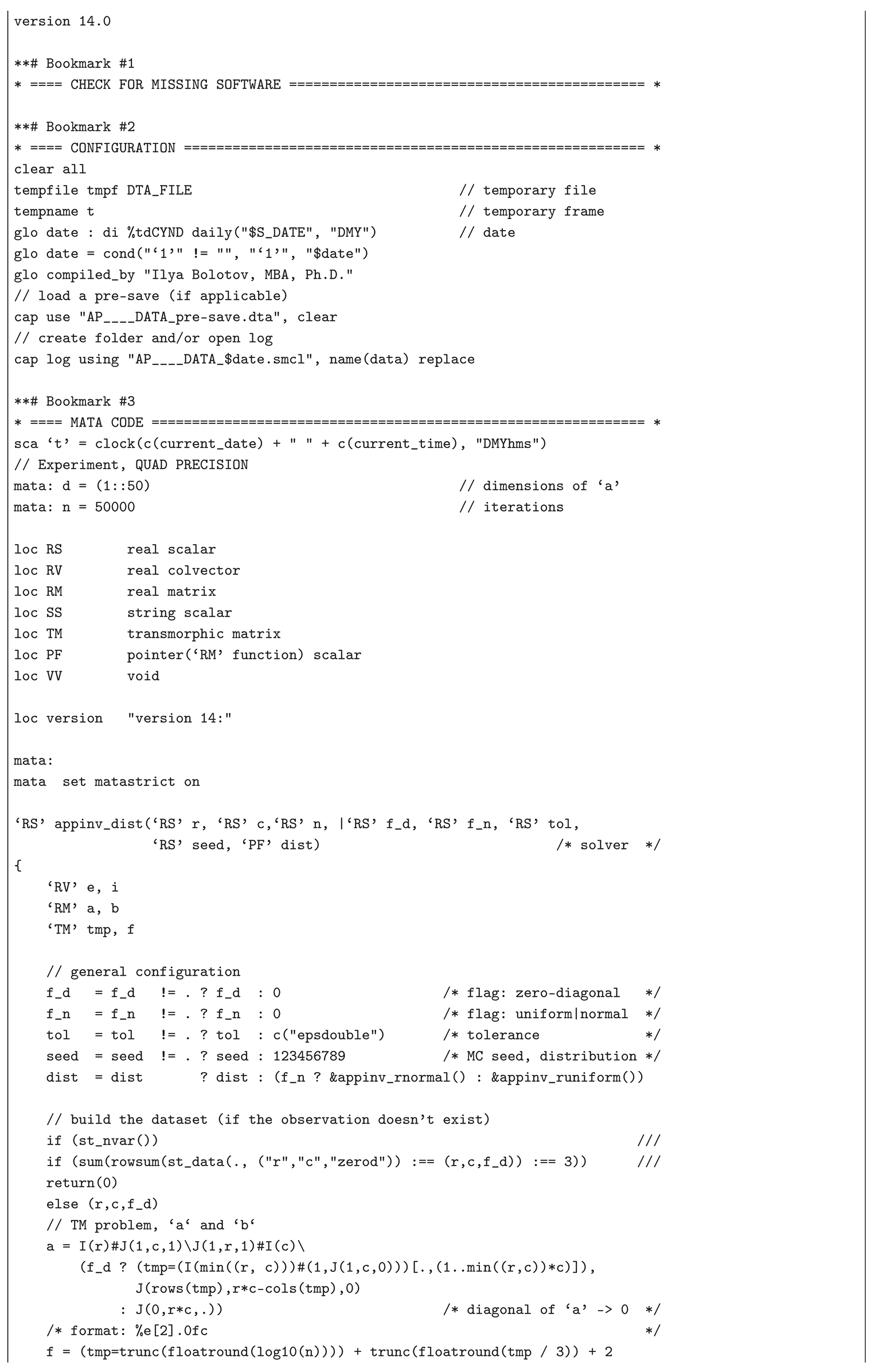
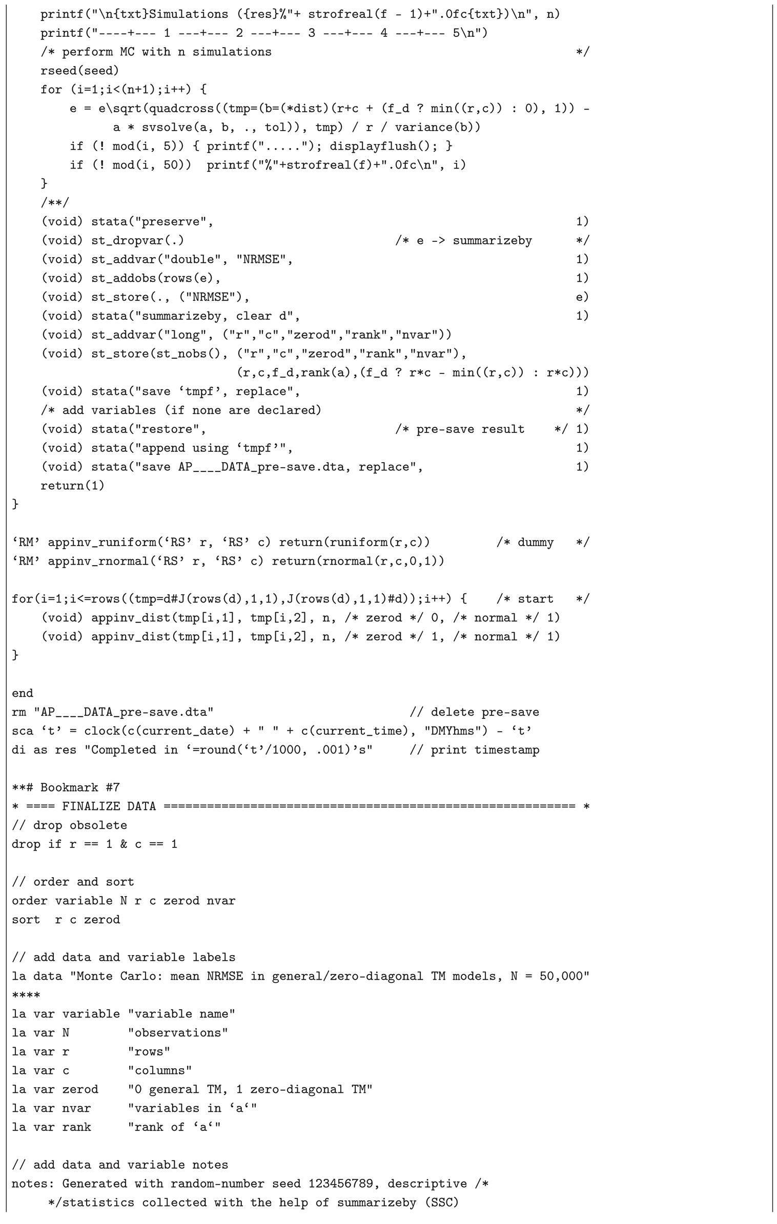
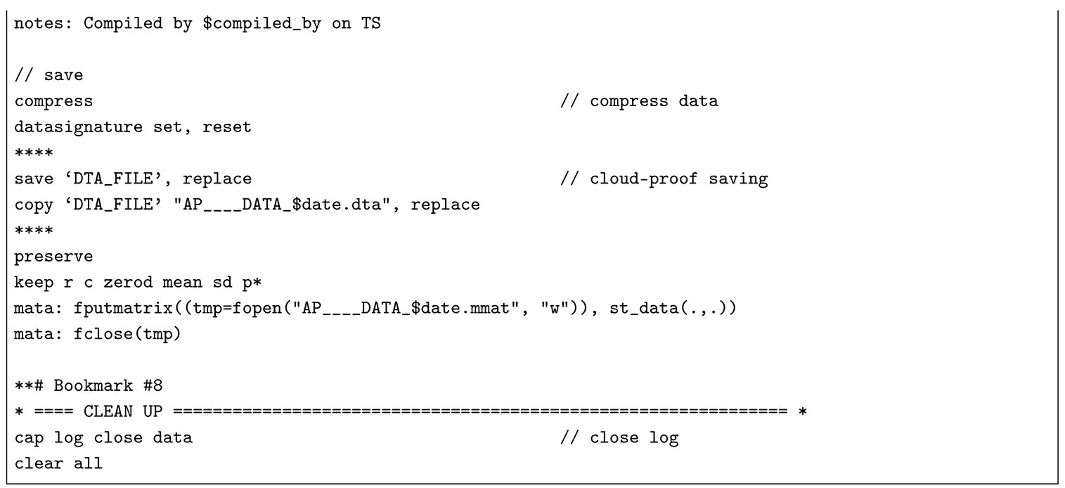
The Monte Carlo experiment and the simulated examples presented below illustrate the applicability of the CLSP to the AP (TM), CMLS (RP), and LPRLS/QPRLS problems. The standardized form of in the APs (TMs), i.e., , with given and r, enables large-scale simulation of the distribution of NRMSE — a robust goodness-of-fit metric for the CLSP — through repeated random trials under varying matrix dimensions , row and column group sizes i and j, and composition of , inferring asymptotic percentile means and standard deviations for practical implementations (e.g., the t-test for the mean). This text presents the results of a simulation study on the distribution of the NRMSE from the first-step estimate (implementable in standard econometric software without CLSP modules) for , , , , and , conducted in Stata/MP (set to version 14.0) with the help of Mata’s 128-bit floating-point cross-product-based quadcross() for greater precision and SVD-based svsolve() with a strict tolerance of c("epsdouble") for increased numerical stability, and a random-variate seed 123456789 (see Appendix B.1 containing a list of dependencies [97] and the Stata .do-file). In this 50,000-iterations Monte Carlo simulation study, spanning matrix dimensions from 1×2 and 2×1 up to 50×50, random normal input vectors were generated for each run, applied with and without zero diagonals (i.e., if, under , is reshaped into a ()-matrix , then ). Thus, a total of 249.9 million observations () was obtained via the formula , resulting in 4,998 aggregated statistics of the asymptotic distribution, assuming convergence: mean, sd, skewness, kurtosis, min, max, as well as p1–p99, as presented in Figure 6 (depicting the intensity of its first two moments, mean and sd) and Table 2 (reporting a subset of all thirteen statistics for ).
From the results of the Monte Carlo experiment, it is observable that: (1) the NRMSE from the first-step estimate and its distributional statistics exhibit increasing stability and boundedness as matrix dimensions increase — specifically, for , both the mean and sd of NRMSE tend to converge, indicating improved estimator performance (e.g., under no diagonal restrictions, at , and , while at , and ); (2) the zero-diagonal constraints () reduce the degrees of freedom and lead to a much more uniform and dimensionally stable distribution of NRMSE across different matrix sizes (e.g., at , mean drops to and sd to , while at , mean rises slightly to and sd to ); and (3) the distribution of NRMSE exhibits mild right skew and leptokurtosis — less so for the zero-diagonal case: under no diagonal restriction, the average skewness is with a coefficient of variation of (i.e., ), and the average kurtosis is with a variation of ; whereas under the zero-diagonal constraint, skewness averages with only variation, and kurtosis averages with variation (i.e., ). To sum up, the larger and less underdetermined (i.e., in an AP (TM) problem, the larger the block of ) the canonical system , the lower the estimation error (i.e., the mean NRMSE) and its variance, and, provided a stable limiting law for NRMSE exists, the skewness and kurtosis from the simulations drift toward 0 and 3, respectively, consistent with — but not proving — a convergence toward a standard-normal distribution.
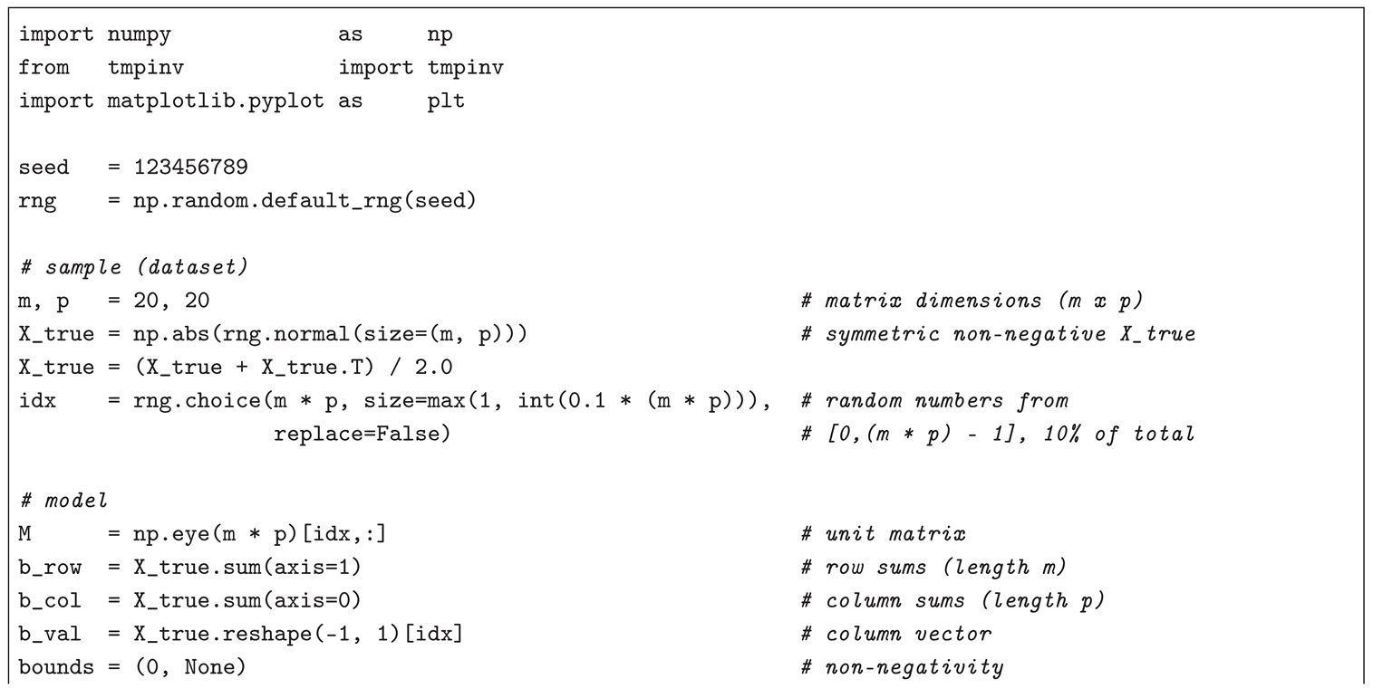
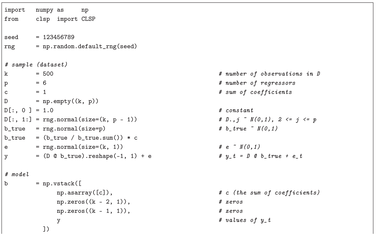
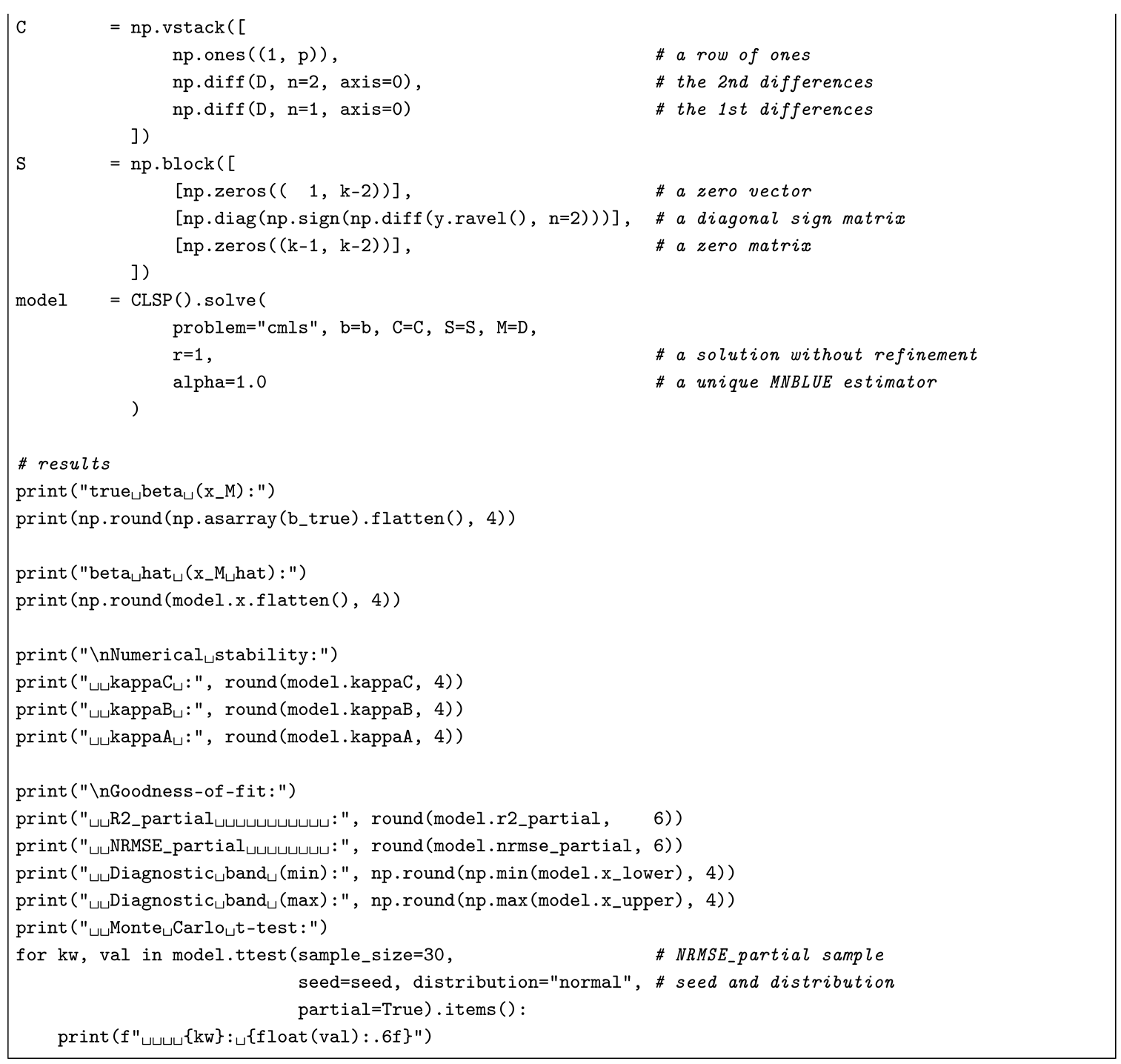
For an illustration of the applicability of the CLSP to the APs (TMs), CMLS (RPs), and LPRLS/QPRLS, the author-developed cross-platform Python 3 module, pyclsp (version ≥ 1.3.0, available on PyPI) [98], — together with its interface co-modules for the APs (TMs), pytmpinv (version ≥ 1.2.0, available on PyPI) [99], and the LPRLS/QPRLS, pylppinv (version ≥ 1.3.0, available on PyPI) [100] (a co-module for the CMLS (RPs) is not provided, as the variability of within the , , block of prevents efficient generalization), — is employed for a sample (dataset) of i random elements (scalars, vectors, or matrices depending on context) and their transformations, drawn independently from the standard normal distribution, i.e., , under the mentioned random-variate seed 123456789 (configured for consistency with the above-described Monte Carlo experiment). Thus, using the cases of (a) a (non-negative symmetric) input-output table and (b) a (non-negative) zero-diagonal trade matrix as two AP (TM) numerical examples, this text simulates problems similar to the ones addressed in Pereira-López et al. [95] and Bolotov [16]: an underdetermined is estimated — from row sums, column sums, and k known values of two randomly generated matrices (a) and (b) , , subject to (a) and (b) — via CLSP assuming , , , and . The Python 3 code, based on pytmpinv and two other modules, installable by executing pip install matplotlib numpy pytmpinv==1.2.0, for (a) and and (b) — estimated with the help of -MNBLUE across reduced models assuming an estimability constraint of — and , with a non-iterated (), unique (), and MNBLUE () (two-step) CLSP solution, is implemented in (a) Listing and (b) Listing (e.g., to be executed in a Jupyter Notebook).
| Listing 1. Simulated numerical example for a symmetric input-output-table-based AP (TM) problem. |
 |
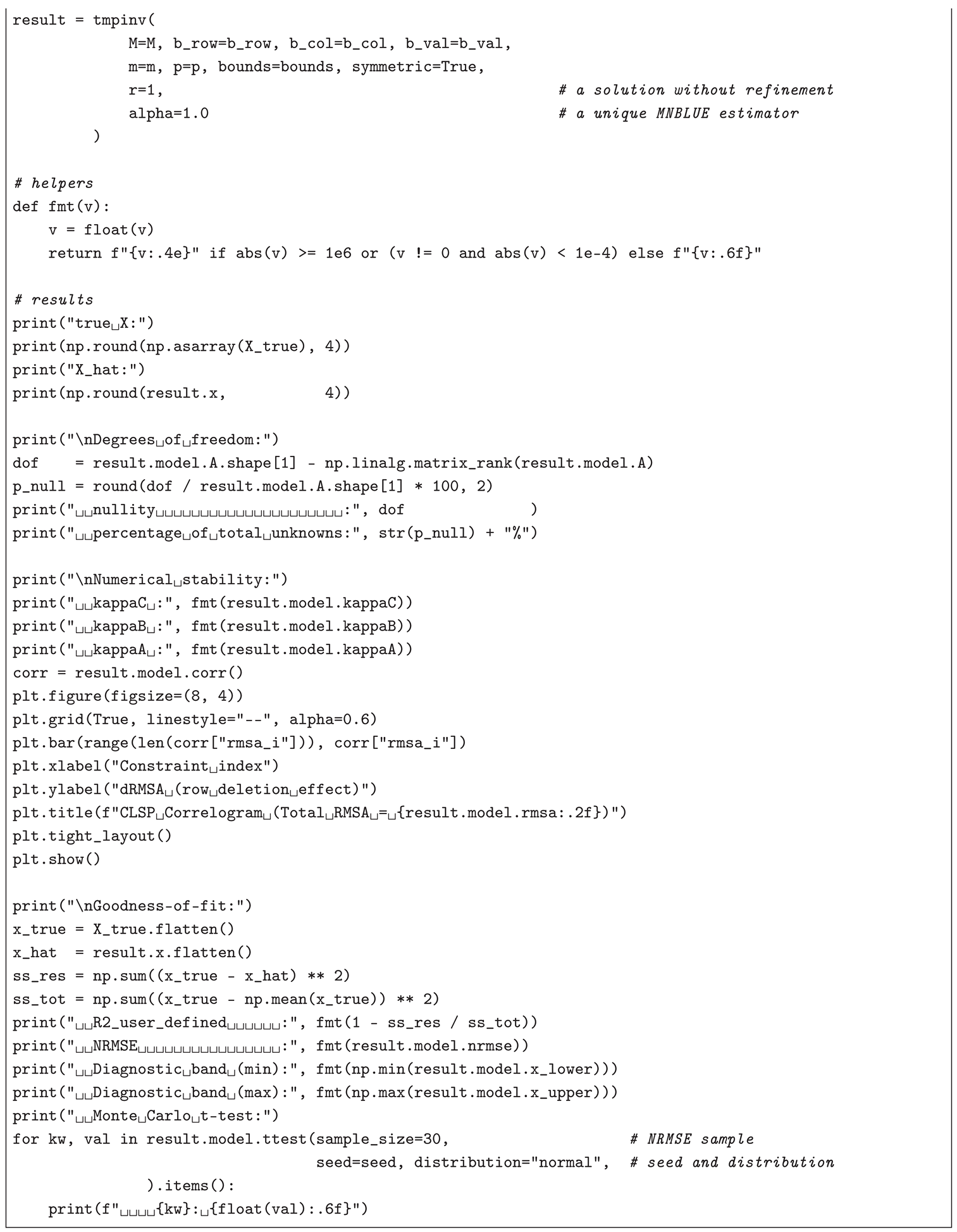 |
In case (a) (see Listing for code), the number of model (target) variables is with a nullity of , corresponding to 80.25% of the total unknowns. Given the simulation of , a matrix unknown in real-world applications, — i.e., CLSP is used to estimate the elements of an existing matrix from its row sums, , column sums, , and a randomly selected 10% of its entries, , — the model’s goodness of fit can be measured by a user-defined (i.e., CLSP achieves an improvement of over a hypothetical naïve predictor reproducing the known 10% entries of and yielding a , but still a modest value of , i.e. a relatively large error, ) with lying within wide condition-weighted diagnostic intervals reflecting the ill-conditioning of the strongly rectangular , , and only the left-sided Monte Carlo-based t-test for the mean of the NRMSE (on a sample of 30 NRMSE values obtained by substituting with ) suggesting consistency with expectations (i.e., with the ). In terms of numerical stability, with a low , as confirmed by the correlogram produced in matplotlib, indicating a well-chosen constraints matrix, even given the underdeterminedness of the model (which also prevents a better fit).
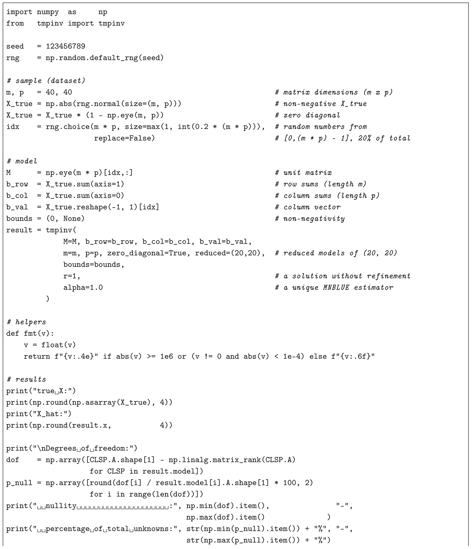
| Listing 2. Simulated numerical example for a (non-negative) trade-matrix-based AP (TM) problem. |
 |
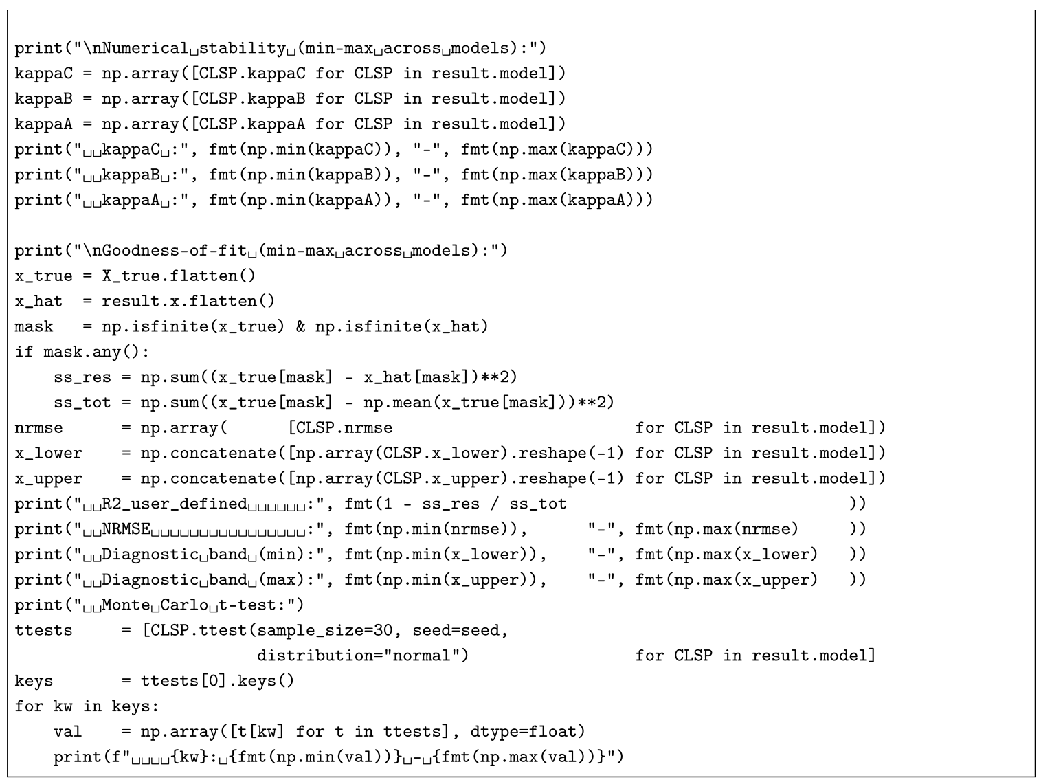 |
In case (b) (see Listing for code), the corresponding number of model (target) variables in each of the reduced design submatrices , , is — where and , one row and one column being reserved for and , which enter as and the vector of slack variables , so that (i.e., the slack matrix compensates for the unaccounted row and column sums in the reduced models as opposed to the full one, such as case (a)) — with a nullity (per reduced model), corresponding to 25.00%–72.68% of the total unknowns (per reduced model) — to compare, a full model, under the same inputs and no computational constraints (i.e., ), would have a nullity , corresponding to 73.00% of the total unknowns. In the examined example, — based on , , and a randomly selected 20% of entries of the true matrix , — the reduced-model block solution’s goodness of fit could not be efficiently measured by a user-defined (i.e., the block matrix constructed from reduced-model estimates led to , but to an error proportionate to the one in case (a), (per reduced model)) — in contrast, a full model would achieve , but at a cost of a greater error, — with lying within strongly varying condition-weighted diagnostic intervals , where (per reduced model) and (per reduced model), and varying results of Monte Carlo-based t-tests for the mean of the (on a sample of 30 values obtained by substituting with ), where p-values range –1.000000 (left-sided), 0.000000–1.000000 (two-sided), and –1.000000 (right-sided) (per reduced model) — alternatively, a full model would lead to wider condition-weighted diagnostic intervals (i.e., reflecting the ill-conditioning of the strongly rectangular , ) and only the left-sided Monte Carlo-based t-test for the mean of the NRMSE (on a sample of 30 NRMSE values obtained by substituting with ) suggesting consistency with expectations (i.e., with the ). In terms of numerical stability, (per reduced model), which indicates well-conditioning of all the reduced models — conversely, in a full model, (therefore, a full model ensures an overall better fit but a lower fit quality, i.e., a trade-off).
As the CMLS (RP) numerical example, this text addresses a problem similar to the one solved in Bolotov [15], Bolotov [96]: a coefficient vector from a (time-series) linear regression model in its classical (statistical) notation with denoting n-th order differences (i.e., the discrete analogue of ) — where is the dependent variable, is the vector of regressors with a constant, is the model’s error (residual), c is a constant, and is the set of stationary points — is estimated on a simulated sample (dataset) with the help of CLSP assuming and , . The Python 3 code, based on numpy and pyclsp modules, installable by executing pip install numpy pyclsp==1.3.0, for , , , , where , , , , , , , , , and , with a non-iterated (), unique (), and MNBLUE () two-step CLSP solution (consistent with the ones from cases (a) and (b) for APs (TMs)), is implemented in Listing (e.g., for a Jupyter Notebook).
| Listing 3. Simulated numerical example for a (time-series) stationary-points-based CMLS (RP) problem. |
 |
 |
Compared to the true values , the CMLS (RP) estimate is with a modest (i.e., a greater error, ), moderate condition-weighted diagnostic intervals , and only the right-sided Monte Carlo-based t-test for the mean of the (on a sample of 30 values obtained by substituting with ) — in the example under scrutiny, is preferable to NRMSE due to — suggesting consistency with expectations (i.e., with the ). Similarly, in terms of numerical stability, , indicating that the constraint block is ill-conditioned, most likely, because of the imposed data- (rather than theory-) based definition of stationary points, which rendered Step 2 infeasible () (limiting the fit quality).
Finally, in the case of a LPRLS/QPRLS numerical example, this text simulates potentially ill-posed LP (QP) problems, similar to the ones addressed in Whiteside et al. [93] and Blair [76], Blair [94]: a solution in its classical LP (QP) notation (), — where is a symmetric positive definite matrix, , , and — is estimated from two randomly generated (coefficient) matrices , , and , , and two (right-hand-side) vectors , , and , , via CLSP assuming , , and , where and are permutation matrices, while omitting and . The Python 3 code, based on numpy and pylppinv modules, installable by executing pip install numpy pylppinv==1.3.0, for , , and , with a non-iterated (), unique (), and MNBLUE () (two-step) CLSP solution (analogously consistent with the ones from cases (a) and (b) for APs (TMs) and the one from CMLS (RPs)), is implemented in Listing (e.g., for a Jupyter Notebook).
| Listing 4. Simulated numerical example for a underdetermined and potentially infeasible LP (QP) problem. |
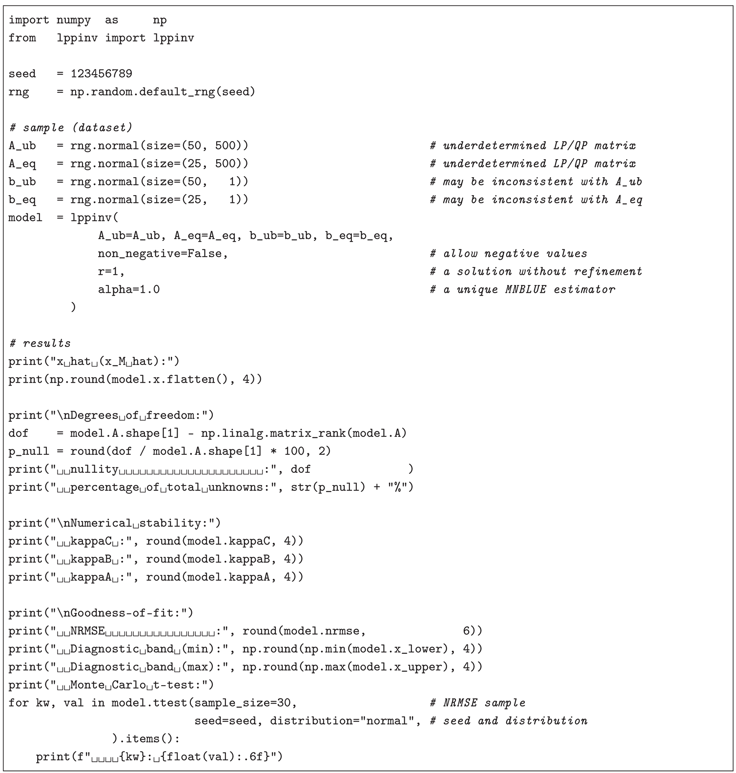 |
The nullity (i.e., underdeterminedness) of the CLSP design matrix, , is , corresponding to 86.36% of the total unknowns, accompanied by a greater (relatively high) error, , moderate condition-weighted diagnostic intervals , and only the right-sided Monte Carlo-based t-test for the mean of the NRMSE (on a sample of 30 NRMSE values obtained by substituting with ) suggesting consistency with expectations (i.e., with the ). Similarly, in terms of numerical stability, , indicating that the constraint block is well-conditioned despite a strongly rectangular . Hence, CLSP can be efficiently applied to AP (TM), CMLS (RP), and LPRLS/QPRLS special cases using Python 3, and the reader may wish to experiment with the code in Listings – by relaxing its uniqueness (setting ) or the MNBLUE characteristic (setting ).
8. Discussion and Conclusions
The proposed modular two-step Convex Least Squares Programming (CLSP) estimator attempts to supersede historical efforts developed mainly in the 1960s–1990s to address ill-posed problems in both LS and LP (QP) — namely, the mentioned Wolfe [84], Stoer [80], Waterman [81], Dax [85], Osborne [78], George and Osborne [79], Barnes et al. [86], Donoho and Tanner [77], Grafarend and Awange [82], Bei et al. [87], and Qian et al. [83] — by correcting (1) the estimation, based on a Moore-Penrose pseudoinverse (which has already been applied in an ad hoc manner in the field, particularly in econometrics in the 2010s; consult Pereira-López et al. [95] and Bolotov [16]) and a Bott-Duffin inverse (based on the literature research, this text may be the first to consider a constrained generalized inverse to generalize an -based estimator) with the help of a (2) regularization-based correction [4] (pp. 477–479), achieving greater fit quality in terms of ensuring strict satisfaction of problem constraints (previously infeasible under an -based solution), while yielding a (potentially) unique and MNBLUE solution (by setting ). At the same time, CLSP is well grounded in the algorithmic logic of the works in question, such as Wolfe [84] and Dax [85], as further formalized by, e.g., Osborne [78]. However, the primary strength of the framework in question lies in its “generality”: in contrast to the (individual) problem-specific algorithms, such as the ones developed by Übi [88], Übi [89], Übi [90], Übi [91], Übi [92] — routines combining (NN)LS, LP, and QP within a single framework to solve both well- and ill-posed convex optimization problems, — CLSP provides a unified estimator with a proper methodology for numerical stability and goodness-of-fit assessment, centered around RMSA and NRMSE. A secondary strength is its practical “versatility”: through at least three classes of special cases — APs (TMs), CMLS (RPs), and LPRLS/QPRLS, — it allows estimation of (rectangular) input-output tables (national, inter-country, or satellite), structural matrices (such as trade, country-product, investment, or migration data), and previously infeasible textbook-definition models of economic variables and/or LP (QP) problems. Furthermore, the inclusion of allows probabilistic and Bayesian applications, since its subspace restrictions can be interpreted in terms of random variables, prior distributions, as well as Monte Carlo-based inference. To conclude, CLSP has already been fully implemented in Python 3 (pyclsp, pytmpinv, and pylppinv) and is to be ported into R and Stata in the future, making it a readily available alternative to purely theoretical or not freely accessible algorithms or proprietary packages, and applicable in a real-world setting (such as econometric research, replacing [15,16,95] with the two-step corrected estimation).
Author Contributions
The manuscript was prepared by a sole author.
Funding
This research received no external funding.
Institutional Review Board Statement
Not applicable.
Informed Consent Statement
Not applicable.
Data Availability Statement
The numerical examples used in the manuscript are based on simulated data. The Python 3.10 and Stata 14 code for replication purposes is provided in Listings – and .
Acknowledgments
All arguments, structure, and conclusions in this manuscript are the author’s own. During the preparation of the manuscript, the author recurred to ChatGPT-5 (OpenAI) solely to improve clarity and language, including refinement of style, formal precision in proofs of theorems, and assistance with interpretation of data and results. No content was adopted without the author’s review and editing, and the author claims full responsibility for the final content of the manuscript.
Conflicts of Interest
The author declares no conflicts of interest.
Abbreviations
The following abbreviations are used in this manuscript (in order of their appearance in the sections):
| CLSP | Convex Least Squares Programming |
| LS | Least Squares |
| OLS | Ordinary Least Squares |
| NNLS | Non-Negative Least Squares |
| SVD | Singular Value Decomposition |
| LP | Linear Programming |
| QP | Quadratic Programming |
| Lasso | Least Absolute Shrinkage and Selection Operator |
| Ridge | Ridge Regression (Tikhonov regularization) |
| MNBLUE | Minimum-Norm Best Linear Unbiased Estimator |
| BLUE | Best Linear Unbiased Estimator |
| RMSA | Root Mean Square Alignment |
| RMSE | Root Mean Square Error |
| NRMSE | Normalized Root Mean Square Error |
| ANOVA | Analysis of Variance |
| CLT | Lindeberg-Lévy Central Limit Theorem |
| APs | Allocation Problems |
| TMs | Tabular Matrix Problems |
| UNCTAD | UN Trade and Development |
| CMLS | Constrained-Model Least Squares |
| RPs | Regression Problems |
| NBER | U.S. National Bureau of Economic Research |
| LPRLS | Linear Programming via Regularized Least Squares |
| QPRLS | Quadratic Programming via Regularized Least Squares |
| iid | independent and identically distributed |
Appendix A
This appendix presents (a) an equation of the Bott-Duffin inverse, , based on the singular value decomposition (SVD), as well as (b) a partitioned decomposition of .
Appendix A.1
Let be a real matrix, and let be a symmetric idempotent matrix (i.e., ) defining a subspace restriction. Then, the Bott-Duffin inverse is given by the formula , as defined in Equation (5), where the projected Gram matrix is computable via its SVD:
where are orthogonal (since the projected Gram matrix is symmetric positive semidefinite, ), and contains the singular values. Hence, for , substitutes :
Appendix A.2
Let in the analysis of numerical stability of the first estimate , as defined in Equation (2). Then a decomposition of reveals how the interaction of constraints and slack structure forms the curvature of the solution space:
While the block captures the contribution of the constraints and reflects the curvature introduced by slack variables, the off-diagonal blocks and encode cross-interactions between constraints and slacks: if these off-diagonal blocks vanish, the effects are orthogonal and additive (in the column space sense since implies ); otherwise, is orthogonalized with respect to , which is effected by . Hence, the presence of in can improve or worsen the ill-posedness of the canonized problem: namely, tends to worsen the condition number .
Appendix B
This appendix presents Stata code, i.e., a .do-file, for the Monte Carlo experiment, compatible with version 14.0 and above (Stata/MP with at least four CPUs is recommended for replication — specifically, 50,000 iterations require substantial CPU time and memory).
- Stata/MP 14.0 dependencies:
- TITLE
’SUMMARIZEBY’: module to use statsby functionality with summarize
- DESCRIPTION/AUTHOR(S)
This routine combines the summarize command with statsby. It iteratively collects summarize results for each variable with statsby and saves the result to memory or to a Stata .dta file.
KW: data management
KW: summarize
KW: statsby
Requires: Stata version 8
Distribution–Date: 20221012
Author: Ilya Bolotov, Prague University of Economics and Business
Support: email ilya.bolotov@vse.cz
- INSTALLATION FILES
summarizeby.ado
summarizeby.sthlp
- (type ssc install summarizeby to install)
Appendix B.1
| Listing B.1. Stata code from the Monte Carlo experiment dedicated to mapping the distribution of NRMSE. |
 |
 |
 |
 |
References
- Nocedal, J.; Wright, S.J. Numerical Optimization, 2 ed.; Springer Series in Operations Research; Springer: New York, NY, 2006; p. 664. [Google Scholar] [CrossRef]
- Boyd, S.; Vandenberghe, L. Convex Optimization, 1 ed.; Cambridge University Press: Cambridge, 2004; p. 727. [Google Scholar] [CrossRef]
- Sydsæter, K.; Hammond, P.; Seierstad, A.; Strøm, A. Further Mathematics for Economic Analysis, 2 ed.; FT Prentice Hall: Harlow; München, 2011; p. 616.
- Gentle, J.E. Matrix Algebra: Theory, Computations and Applications in Statistics, 3 ed.; Springer Texts in Statistics, Springer: Cham, 2024; p. 725. [Google Scholar] [CrossRef]
- Dantzig, G.B. Reminiscences about the Origins of Linear Programming. Memoirs of the American Mathematical Society 1984, 48, 1–11. [Google Scholar] [CrossRef]
- Dantzig, G.B. Linear Programming and Extensions, 1 (reprint of 1963) ed.; Princeton Landmarks in Mathematics and Physics, Princeton University Press: Princeton, NJ, 1998; p. 656. [Google Scholar]
- Koopmans, T.C. Activity Analysis of Production and Allocation: Proceedings of a Conference, 1 ed.; Wiley: New York, NY, 1951; p. 404. [Google Scholar]
- Allen, R.G.D. Mathematical Economics, 2 (reprint of 1959) ed.; Palgrave Macmillan: London, 1976; p. 812. [Google Scholar] [CrossRef]
- Lancaster, K. Mathematical Economics, 1 ed.; Dover Publications: New York, NY, 1987; p. 411. [Google Scholar]
- Intriligator, M.D. Mathematical Optimization and Economic Theory, 1 (reprint of 1971) ed.; Classics in Applied Mathematics, SIAM: Philadelphia, PA, 2002; p. 508. [Google Scholar] [CrossRef]
- Intriligator, M.D.; Arrow, K.J. Handbook of Mathematical Economics, 1 ed.; Handbooks in Economics, North-Holland: Amsterdam; New York, NY, 1981; p. 378.
- Dorfman, R.; Samuelson, P.A.; Solow, R.M. Linear Programming and Economic Analysis, 1 (reprint of 1958) ed.; Dover Books on Advanced Mathematics, Dover Publications: New York, NY, 1987; p. 525. [Google Scholar]
- Frühwirth, T.; Abdennadher, S. Essentials of Constraint Programming, 1 ed.; Cognitive Technologies, Springer: Berlin; Heidelberg, 2003; p. 144. [CrossRef]
- Rossi, F.; van Beek, P.; Walsh, T., Eds. Handbook of Constraint Programming, 1 ed.; Vol. 2, Foundations of Artificial Intelligence, Elsevier: Amsterdam; Boston, MA, 2006; p. 955.
- Bolotov, I. Modeling of Time Series Cyclical Component on a Defined Set of Stationary Points and Its Application on the U.S. Business Cycle. In Proceedings of the The 8th International Days of Statistics and Economics. Melandrium, Sep 11–13 2014, pp. 151–160.
- Bolotov, I. Modeling Bilateral Flows in Economics by Means of Exact Mathematical Methods. In Proceedings of the The 9th International Days of Statistics and Economics. Melandrium, Sep 10–12 2015; pp. 199–208. [Google Scholar]
- Rosenthal, A. The History of Calculus. The American Mathematical Monthly 1951, 58, 75–86. [Google Scholar] [CrossRef]
- Stigler, S.M. The History of Statistics: The Measurement of Uncertainty Before 1900, 1 (reprint of 1986) ed.; Harvard University Press: Cambridge, MA, 2003; p. 410. [Google Scholar]
- Ok, E.A. Real Analysis with Economic Applications, 1 ed.; Princeton University Press: Princeton, NJ, 2007; p. 802. [Google Scholar]
- Creedy, J. The Early Use of Lagrange Multipliers in Economics. The Economic Journal 1980, 90, 371–376. [Google Scholar] [CrossRef]
- Plackett, R.L. Studies in the History of Probability and Statistics. XXIX: The Discovery of the Method of Least Squares. Biometrika 1972, 59, 239. [Google Scholar] [CrossRef]
- Stigler, S.M. Gauss and the Invention of Least Squares. Annals of Statistics 1981, 9, 465–474. [Google Scholar] [CrossRef]
- Stigler, S.M. Statistics on the Table: The History of Statistical Concepts and Methods, 1 (reprint of 1999) ed.; Harvard University Press: Cambridge, MA, 2002; p. 488. [Google Scholar]
- Aitken, A.C. IV. —On Least Squares and Linear Combination of Observations. Proceedings of the Royal Society of Edinburgh 1936, 55, 42–48. [Google Scholar] [CrossRef]
- Aldrich, J. Doing Least Squares: Perspectives from Gauss and Yule. International Statistical Review 1998, 66, 61–81. [Google Scholar] [CrossRef]
- Mills, T.C.; Patterson, K., Eds. Palgrave Handbook of Econometrics: Volume 1: Econometric Theory, 1 ed.; Palgrave Macmillan: Basingstoke; New York, NY, 2006; p. 1097.
- Mills, T.C.; Patterson, K., Eds. Palgrave Handbook of Econometrics: Volume 2: Applied Econometrics, 1 ed.; Palgrave Macmillan: Basingstoke; New York, NY, 2009; p. 1385.
- Golub, G.H.; Kahan, W. Calculating the Singular Values and Pseudo-Inverse of a Matrix. SIAM Journal on Numerical Analysis 1965, 2, 205–224. [Google Scholar] [CrossRef]
- Eldén, L. A Weighted Pseudoinverse, Generalized Singular-Values, and Constrained Least-Squares Problems. BIT Numerical Mathematics 1982, 22, 487–502. [Google Scholar] [CrossRef]
- Ward, J.F. Limit Formula for Weighted Pseudoinverses. SIAM Journal on Applied Mathematics 1977, 33, 34–38. [Google Scholar] [CrossRef]
- Barata, J.C.A.; Hussein, M.S. The Moore-Penrose Pseudoinverse: A Tutorial Review of the Theory. Brazilian Journal of Physics 2012, 42, 146–165. [Google Scholar] [CrossRef]
- Tikhonov, A.N.; Goncharskiy, A.V.; Stepanov, V.V.; Yagola, A.G. Chislennyye metody resheniya nekorrektnykh zadach, 2 ed.; Nauka: Moscow, 1990; p. 232. [Google Scholar]
- Rao, C.R.; Mitra, S.K. Generalized Inverse of Matrices and Its Applications, 1 ed.; Wiley Series in Probability and Mathematical Statistics; Wiley: New York, NY, 1971; p. 240. [Google Scholar] [CrossRef]
- Ben-Israel, A.; Greville, T.N.E. Generalized Inverses: Theory and Applications, 2 (reprint of 2003) ed.; CMS Books in Mathematics, Springer: New York, NY, 2006; p. 420. [Google Scholar] [CrossRef]
- Dresden, A. The Fourteenth Western Meeting of the American Mathematical Society. Bulletin of the American Mathematical Society 1920, 26, 385–397. [Google Scholar] [CrossRef]
- Bjerhammar, A. Rectangular Reciprocal Matrices, With Special Reference to Geodetic Calculations. Bulletin géodésique 1951, 20, 188–220. [Google Scholar] [CrossRef]
- Penrose, R. A Generalized Inverse for Matrices. Mathematical Proceedings of the Cambridge Philosophical Society 1955, 51, 406–413. [Google Scholar] [CrossRef]
- Penrose, R. On Best Approximate Solutions of Linear Matrix Equations. Mathematical Proceedings of the Cambridge Philosophical Society 1956, 52, 17–19. [Google Scholar] [CrossRef]
- Chipman, J.S. On Least Squares with Insufficient Observations. Journal of the American Statistical Association 1964, 59, 1078–1111. [Google Scholar] [CrossRef]
- Price, C.M. The Matrix Pseudoinverse and Minimal Variance Estimates. SIAM Review 1964, 6, 115–120. [Google Scholar] [CrossRef]
- Plackett, R.L. Some Theorems in Least Squares. Biometrika 1950, 37, 149–157. [Google Scholar] [CrossRef]
- Rao, C.R.; Mitra, S.K., Generalized Inverse of a Matrix and Its Applications. In Theory of Statistics: Proceedings of the Sixth Berkeley Symposium on Mathematical Statistics and Probability, Volume I, 1 ed.; Le Cam, L.M.; Neyman, J.; Scott, E.L., Eds.; University of California Press: Berkeley, CA, 1972; pp. 601–620.
- Greville, T.N.E. The Pseudoinverse of a Rectangular Matrix and Its Statistical Applications. In Proceedings of the Annual Meeting of the American Statistical Association. American Statistical Association, Dec 27–30 1958; pp. 116–121. [Google Scholar]
- Greville, T.N.E. The Pseudoinverse of a Rectangular or Singular Matrix and Its Application to the Solution of Systems of Linear Equations. SIAM Review 1959, 1, 38–43. [Google Scholar] [CrossRef]
- Greville, T.N.E. Some Applications of the Pseudoinverse of a Matrix. SIAM Review 1960, 2, 15–22. [Google Scholar] [CrossRef]
- Greville, T.N.E. Note on Fitting of Functions of Several Independent Variables. Journal of the Society for Industrial and Applied Mathematics 1961, 9, 109–115. [Google Scholar] [CrossRef]
- Cline, R.E. Representations for the Generalized Inverse of a Partitioned Matrix. Journal of the Society for Industrial and Applied Mathematics 1964, 12, 588–600. [Google Scholar] [CrossRef]
- Cline, R.E.; Greville, T.N.E. An Extension of the Generalized Inverse of a Matrix. SIAM Journal on Applied Mathematics 1970, 19, 682–688. [Google Scholar] [CrossRef]
- Ben-Israel, A.; Cohen, D. On Iterative Computation of Generalized Inverses and Associated Projections. SIAM Review 1966, 8, 410–419. [Google Scholar] [CrossRef]
- Lewis, T.O.; Newman, T.G. Pseudoinverses of Positive Semidefinite Matrices. SIAM Journal on Applied Mathematics 1968, 16, 701–703. [Google Scholar] [CrossRef]
- Bott, R.; Duffin, R.J. On the Algebra of Networks. Transactions of the American Mathematical Society 1953, 74, 99–109. [Google Scholar] [CrossRef]
- Campbell, S.L.; Meyer, C.D. Generalized Inverses of Linear Transformations, 1 (reprint of 1979) ed.; Classics in Applied Mathematics, SIAM: Philadelphia, PA, 2009; p. 272. [Google Scholar] [CrossRef]
- Wang, G.; Wei, Y.; Qiao, S. Generalized Inverses: Theory and Computations, 1 ed.; Vol. 53, Developments in Mathematics, Springer: Singapore, 2018; p. 397. [Google Scholar] [CrossRef]
- Meyer, Carl D. , J. Generalized Inverses and Ranks of Block Matrices. SIAM Journal on Applied Mathematics 1973, 25, 597–602. [Google Scholar] [CrossRef]
- Hartwig, R.E. Block Generalized Inverses. Archive for Rational Mechanics and Analysis 1976, 61, 197–251. [Google Scholar] [CrossRef]
- Rao, C.R.; Yanai, H. Generalized Inverses of Partitioned Matrices Useful in Statistical Applications. Linear Algebra and Its Applications 1985, 70, 105–113. [Google Scholar] [CrossRef]
- Tian, Y. The Moore-Penrose Inverses of m x n Block Matrices and Their Applications. Linear Algebra and Its Applications 1998, 283, 35–60. [Google Scholar] [CrossRef]
- Rakha, M.A. On the Moore-Penrose Generalized Inverse Matrix. Applied Mathematics and Computation 2004, 158, 185–200. [Google Scholar] [CrossRef]
- Baksalary, O.M.; Trenkler, G. On Formulae for the Moore-Penrose Inverse of a Columnwise Partitioned Matrix. Applied Mathematics and Computation 2021, 403, 1–10. [Google Scholar] [CrossRef]
- Albert, A.E. Regression and the Moore-Penrose Pseudoinverse, 1 ed.; Mathematics in Science and Engineering, Academic Press: New York, NY, 1972; p. 180. [Google Scholar]
- Dokmanić, I.; Kolundžija, M.; Vetterli, M. Beyond Moore-Penrose: Sparse Pseudoinverse. In Proceedings of the IEEE International Conference on Acoustics, Speech, May 26–31 2013, and Signal Processing (ICASSP). IEEE; pp. 6526–6530. [CrossRef]
- Baksalary, O.M.; Trenkler, G. The Moore-Penrose Inverse: A Hundred Years on a Frontline of Physics Research. European Physical Journal H 2021, 46, 1–10. [Google Scholar] [CrossRef]
- Mortari, D. Least-Squares Solution of Linear Differential Equations. Mathematics 2017, 5, 48. [Google Scholar] [CrossRef]
- Lawson, C.L.; Hanson, R.J. Solving Least Squares Problems, 1 (reprint of 1974) ed.; Classics in Applied Mathematics, SIAM: Philadelphia, PA, 1995; p. 337. [Google Scholar] [CrossRef]
- Getson, A.J.; Hsuan, F.C. {2}-Inverses and Their Statistical Application, 1 (reprint of 1988) ed.; Lecture Notes in Statistics, Springer: New York, NY, 2012; p. 110. [Google Scholar] [CrossRef]
- Björck, A. Numerical Methods for Least Squares Problems, 1 ed.; SIAM: Philadelphia, PA, 1996; p. 408. [Google Scholar]
- Kantorovich, L.V. Matematicheskiye metody organizatsii i planirovaniia proizvodstva, , reprint ed.; Izdatel’skiy dom S.-Peterb. gos. un-ta: Saint Petersburg, 2012; p. 96. [Google Scholar]
- Shamir, R. The Efficiency of the Simplex Method: A Survey. Management Science 1987, 33, 301–334. [Google Scholar] [CrossRef]
- Stone, R.E.; Tovey, C.A. The Simplex and Projective Scaling Algorithms as Iteratively Reweighted Least Squares Methods. SIAM Review 1991, 33, 220–237. [Google Scholar] [CrossRef]
- Wagner, H.M. Linear Programming Techniques for Regression Analysis. Journal of the American Statistical Association 1959, 54, 206–212. [Google Scholar] [CrossRef]
- Sielken, R.L.; Hartley, H.O. Two Linear Programming Algorithms for Unbiased Estimation of Linear Models. Journal of the American Statistical Association 1973, 68, 639–641. [Google Scholar] [CrossRef]
- Kiountouzis, E.A. Linear Programming Techniques in Regression Analysis. Applied Statistics 1973, 22, 69. [Google Scholar] [CrossRef]
- Sposito, V.A. On Unbiased Lp Regression Estimators. Journal of the American Statistical Association 1982, 77, 652–653. [Google Scholar] [CrossRef]
- Judge, G.G.; Takayama, T. Inequality Restrictions in Regression Analysis. Journal of the American Statistical Association 1966, 61, 166–181. [Google Scholar] [CrossRef]
- Mantel, N. Restricted Least Squares Regression and Convex Quadratic Programming. Technometrics 1969, 11, 763–773. [Google Scholar] [CrossRef]
- Blair, C. Random Linear Programs with Many Variables and Few Constraints. Mathematical Programming 1986, 34, 62–71. [Google Scholar] [CrossRef]
- Donoho, D.L.; Tanner, J. Sparse Nonnegative Solution of Underdetermined Linear Equations by Linear Programming. Proceedings of the National Academy of Sciences of the United States of America 2005, 102, 9446–9451. [Google Scholar] [CrossRef]
- Osborne, M.R. Degeneracy: Resolve or Avoid? Journal of the Operational Research Society 1992, 43, 829–835. [Google Scholar] [CrossRef]
- George, K.; Osborne, M.R. On Degeneracy in Linear Programming and Related Problems. Annals of Operations Research 1993, 46-47, 343–359. [Google Scholar] [CrossRef]
- Stoer, J. On the Numerical Solution of Constrained Least-Squares Problems. SIAM Journal on Numerical Analysis 1971, 8, 382–411. [Google Scholar] [CrossRef]
- Waterman, M.S. A Restricted Least Squares Problem. Technometrics 1974, 16, 135–136. [Google Scholar] [CrossRef]
- Grafarend, E.W.; Awange, J.L., Algebraic Solutions of Systems of Equations. In Linear and Nonlinear Models, 1 ed.; Springer: Berlin; Heidelberg, 2012; pp. 527–569. [CrossRef]
- Qian, J.; Andrew, A.L.; Chu, D.; Tan, R.C.E. Methods for Solving Underdetermined Systems. Numerical Linear Algebra with Applications 2018, 25, 17. [Google Scholar] [CrossRef]
- Wolfe, P. A Technique for Resolving Degeneracy in Linear Programming. Journal of the Society for Industrial and Applied Mathematics 1963, 11, 205–211. [Google Scholar] [CrossRef]
- Dax, A. Linear Programming via Least Squares. Linear Algebra and Its Applications 1988, 111, 313–324. [Google Scholar] [CrossRef]
- Barnes, E.; Chen, V.; Gopalakrishnan, B.; Johnson, E.L. A Least-Squares Primal-Dual Algorithm for Solving Linear Programming Problems. Operations Research Letters 2002, 30, 289–294. [Google Scholar] [CrossRef]
- Bei, X.; Chen, N.; Zhang, S. Solving Linear Programming with Constraints Unknown. In Proceedings of the 42nd International Colloquium, Jul 6–10 2015, Vol. 9134, ICALP 2015. Springer; pp. 129–142. [Google Scholar] [CrossRef]
- Übi, E. Exact and Stable Least Squares Solution to the Linear Programming Problem. Central European Journal of Mathematics 2005, 3, 228–241. [Google Scholar] [CrossRef]
- Übi, E. On Stable Least Squares Solution to the System of Linear Inequalities. Open Mathematics 2007, 5, 373–385. [Google Scholar] [CrossRef]
- Übi, E. A Numerically Stable Least Squares Solution to the Quadratic Programming Problem. Open Mathematics 2008, 6, 171–178. [Google Scholar] [CrossRef]
- Übi, E. Mathematical Programming via the Least-Squares Method. Open Mathematics 2010, 8. [Google Scholar] [CrossRef]
- Übi, E. Linear Inequalities via Least Squares. Proceedings of the Estonian Academy of Sciences 2013, 62, 238–248. [Google Scholar] [CrossRef]
- Whiteside, M.M.; Choi, B.; Eakin, M.; Crockett, H. Stability of Linear Programming Solutions Using Regression Coefficients. Journal of Statistical Computation and Simulation 1994, 50, 131–146. [Google Scholar] [CrossRef]
- Blair, C. Random Inequality Constraint Systems with Few Variables. Mathematical Programming 1986, 35, 135–139. [Google Scholar] [CrossRef]
- Pereira-López, X.; Fernández-Fernández, M.; Carrascal-Incera, A. Rectangular Input-output Models by Moore-Penrose Inverse. Revista Electrónica De Comunicaciones Y Trabajos De ASEPUMA 2014, 15, 13–24. [Google Scholar]
- Bolotov, I. The Problem of Relationships Between Conditional Statements and Arithmetic Functions. Mundus Symbolicus 2012, 20, 5–12. [Google Scholar]
- Bolotov, I. SUMMARIZEBY: Stata Module to Use Statsby Functionality With Summarize (version 1.1.2), 2022.
- Bolotov, I. PYCLSP: Modular Two-Step Convex Optimization Estimator for Ill-Posed Problems (version 1.3.0), 2025.
- Bolotov, I. PYTMPINV: Tabular Matrix Problems via Pseudoinverse Estimation (version 1.2.0), 2025.
- Bolotov, I. PYLPPINV: Linear Programming via Pseudoinverse Estimation (version 1.3.0), 2025.
Figure 1.
LP and QP in programming. Adapted from Dantzig (1990, Figure 1.4.1, p. 8) [6] (pp. 1–11).
Figure 1.
LP and QP in programming. Adapted from Dantzig (1990, Figure 1.4.1, p. 8) [6] (pp. 1–11).
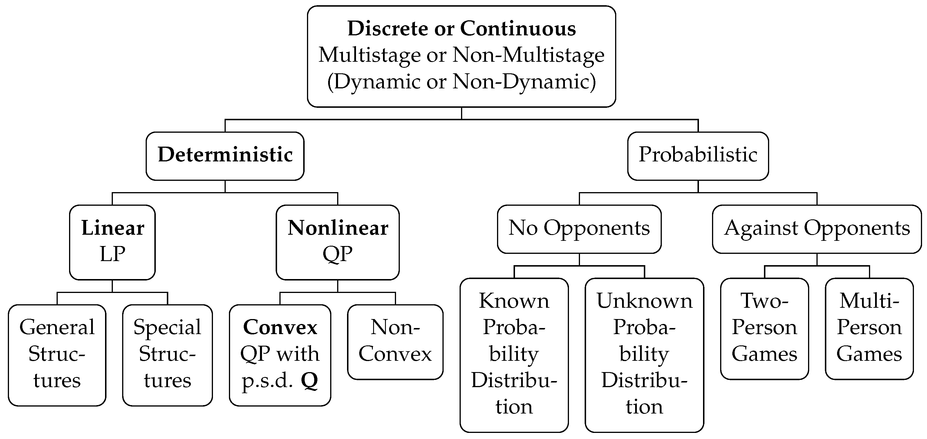
Figure 2.
Applicability of selected types of convex optimization methods across problem classes.
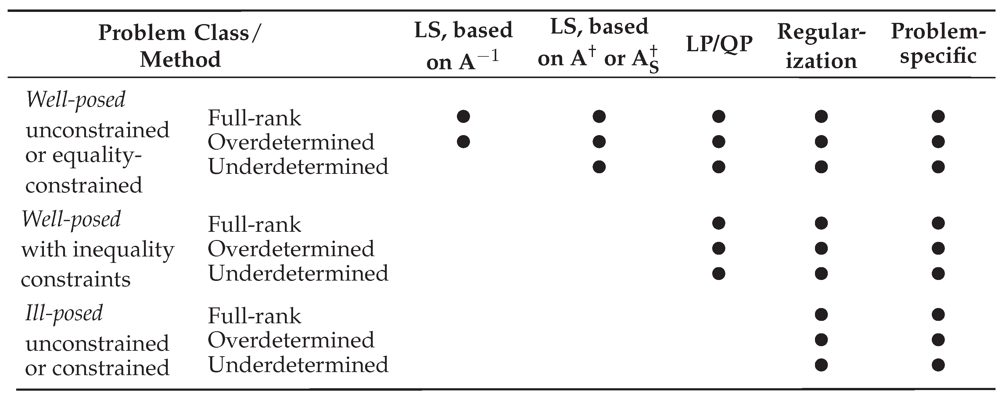
Figure 3.
Map of citation and reference counts for the above-cited sources, where hollow circles are suggested items. Monographs not indexed in the database are denoted as (?). Adapted from Litmaps (Shared Citations & References), available at https://www.litmaps.com/ (accessed on June 30, 2025).
Figure 3.
Map of citation and reference counts for the above-cited sources, where hollow circles are suggested items. Monographs not indexed in the database are denoted as (?). Adapted from Litmaps (Shared Citations & References), available at https://www.litmaps.com/ (accessed on June 30, 2025).
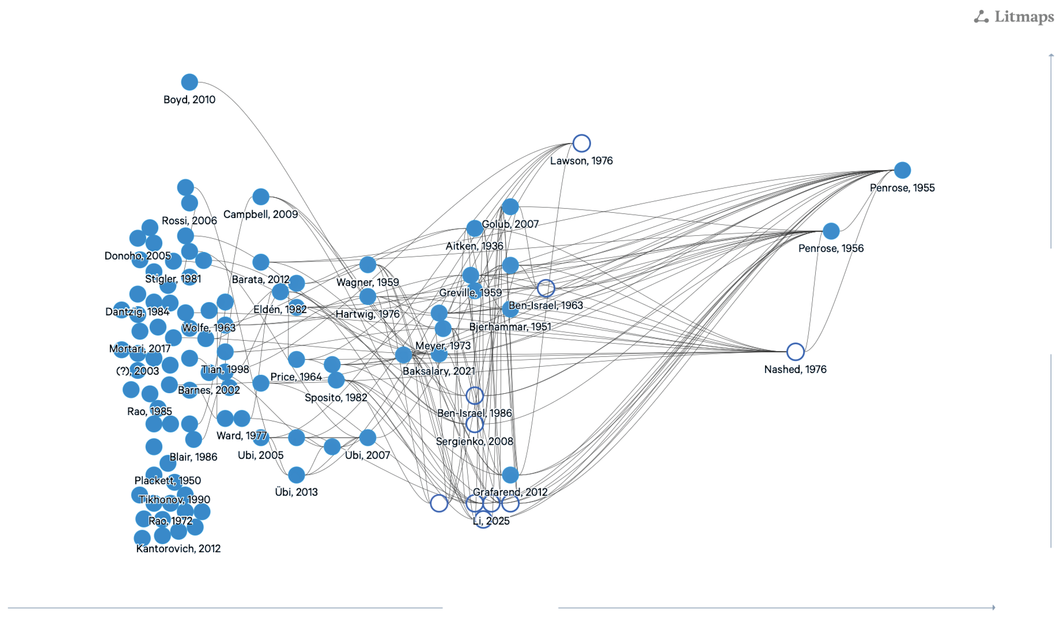
Figure 4.
Algorithmic flow of the CLSP Estimator. Decision nodes (diamonds) indicate modularity.
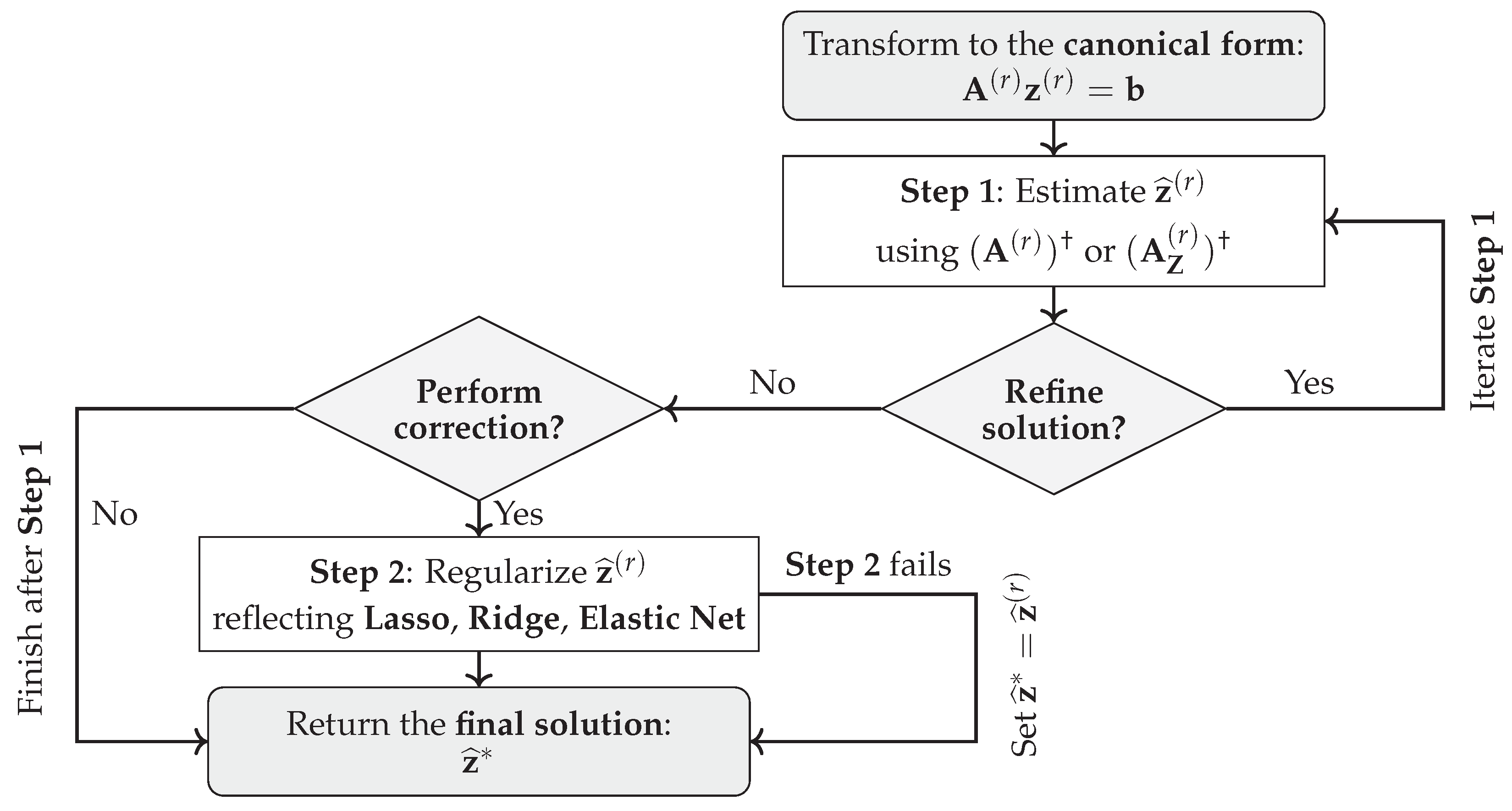
Figure 5.
Schematic correlogram of constraint rows i with high alignment (). Each row encodes directional alignment and symbolic marginal effects on model conditioning and fit.
Figure 5.
Schematic correlogram of constraint rows i with high alignment (). Each row encodes directional alignment and symbolic marginal effects on model conditioning and fit.
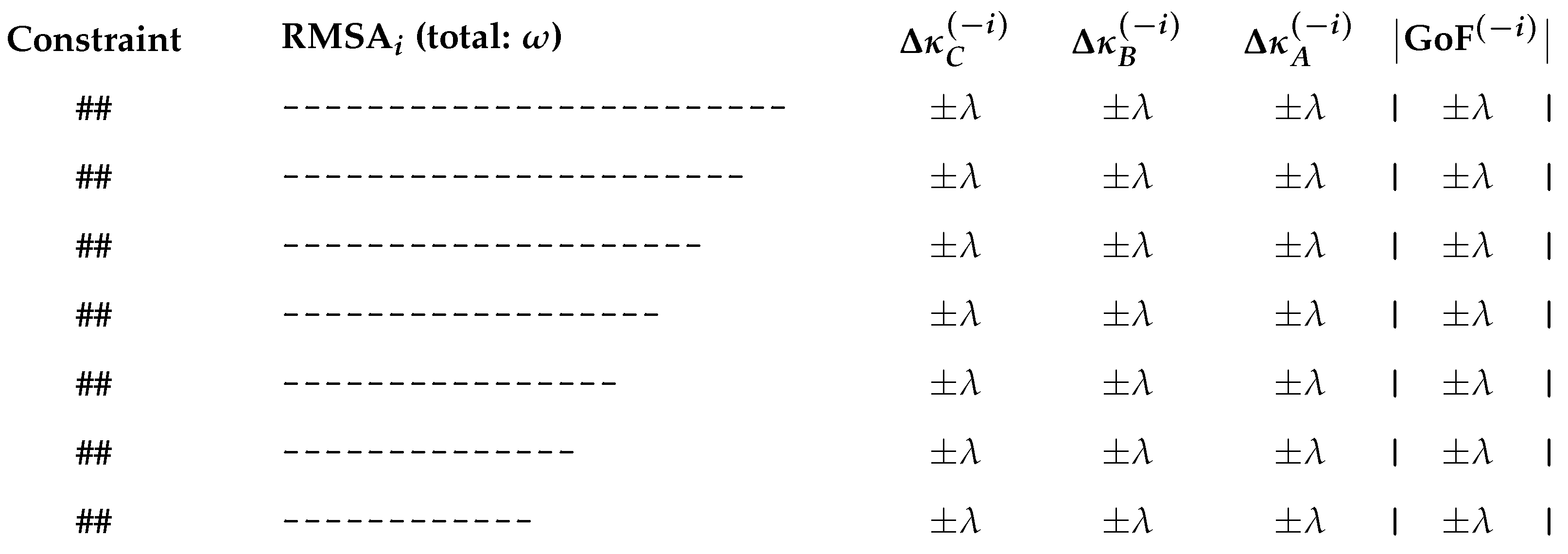
Figure 6.
Heatmaps (based on seaborn’s viridis colormap) of means, , and standard deviations, , computed from the NRMSE of , where , under two structural variants: with and without a zero diagonal (). Color reflects the magnitude of the statistic, with lighter shades indicating higher values. The figure was prepared using matplotlib in Python 3.
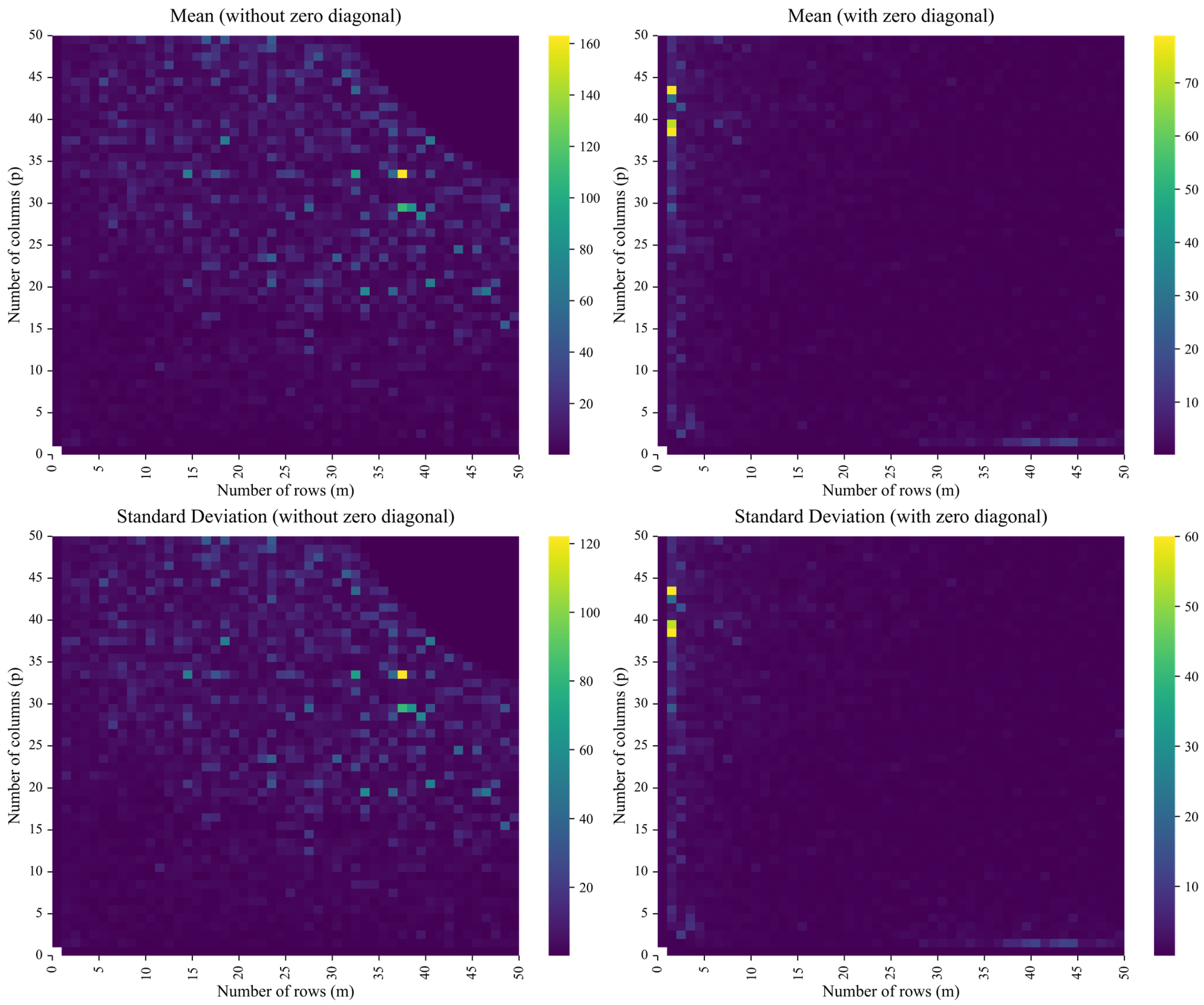

Table 1.
Selected types of generalized inverses , where , , and .
| Type of Inverse | Terminology | Properties |
|---|---|---|
| Equation Solving Inverse | iff . Hence, is a solution to for all . | |
| Reflexive Inverse | iff and . Each -inverse defines a direct sum , . For complementary subspaces , is unique, with and . | |
| Least Squares Inverse | iff and . Hence, is the least-squares solution minimizing the norm . | |
| Minimum Norm Inverse | iff and . Hence, is the minimum-norm solution of for all . | |
| Moore-Penrose Inverse | The unique is the least-squares minimum-norm solution. |
Table 2.
Subset (at ) of the summary statistics for NRMSE from the Simulation Study.
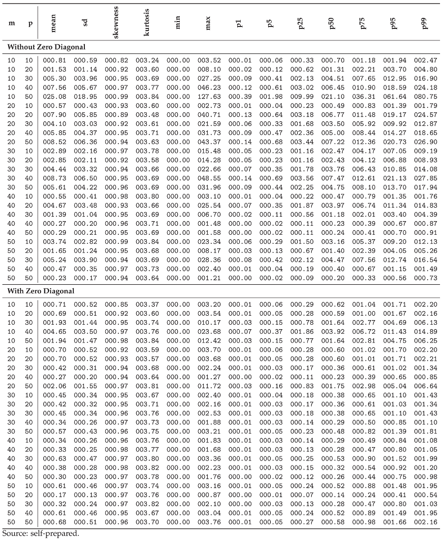 |
Disclaimer/Publisher’s Note: The statements, opinions and data contained in all publications are solely those of the individual author(s) and contributor(s) and not of MDPI and/or the editor(s). MDPI and/or the editor(s) disclaim responsibility for any injury to people or property resulting from any ideas, methods, instructions or products referred to in the content. |
© 2025 by the authors. Licensee MDPI, Basel, Switzerland. This article is an open access article distributed under the terms and conditions of the Creative Commons Attribution (CC BY) license (http://creativecommons.org/licenses/by/4.0/).
Copyright: This open access article is published under a Creative Commons CC BY 4.0 license, which permit the free download, distribution, and reuse, provided that the author and preprint are cited in any reuse.


