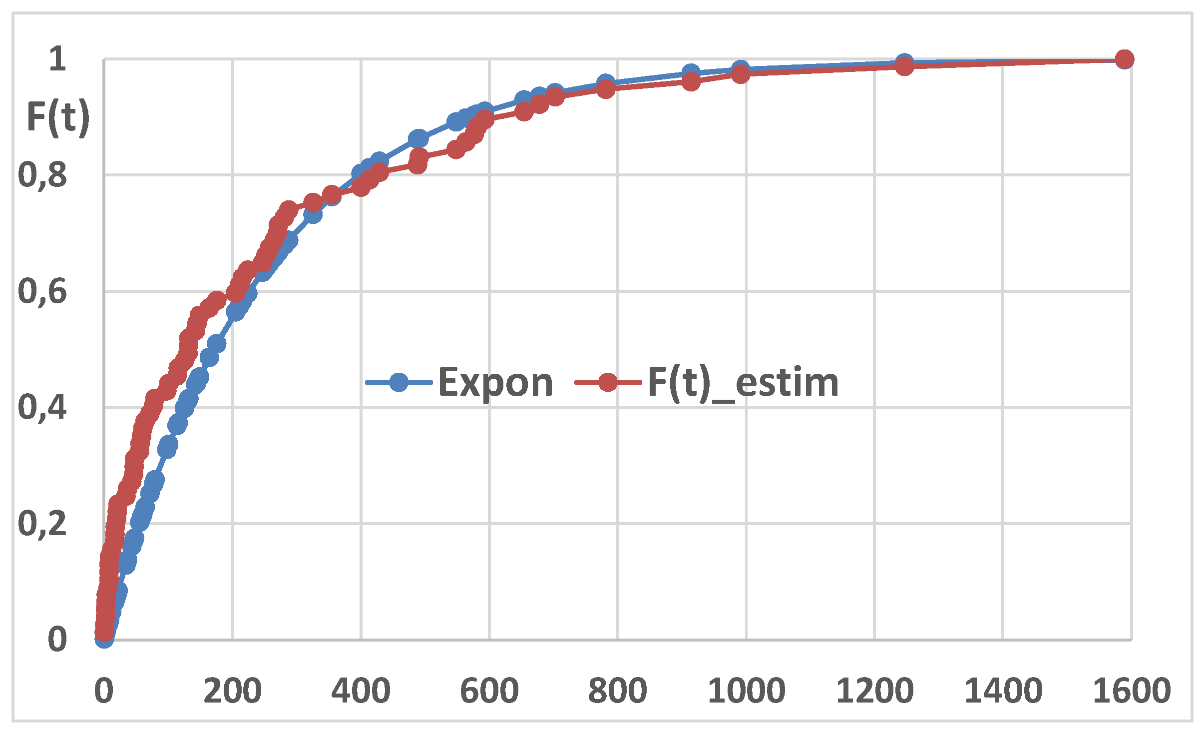
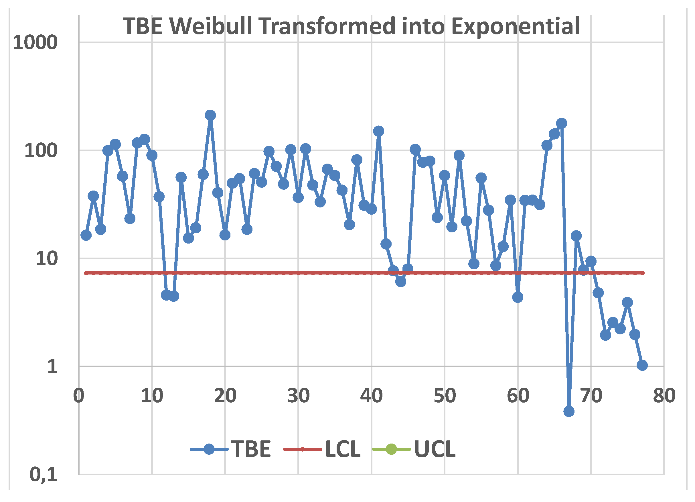
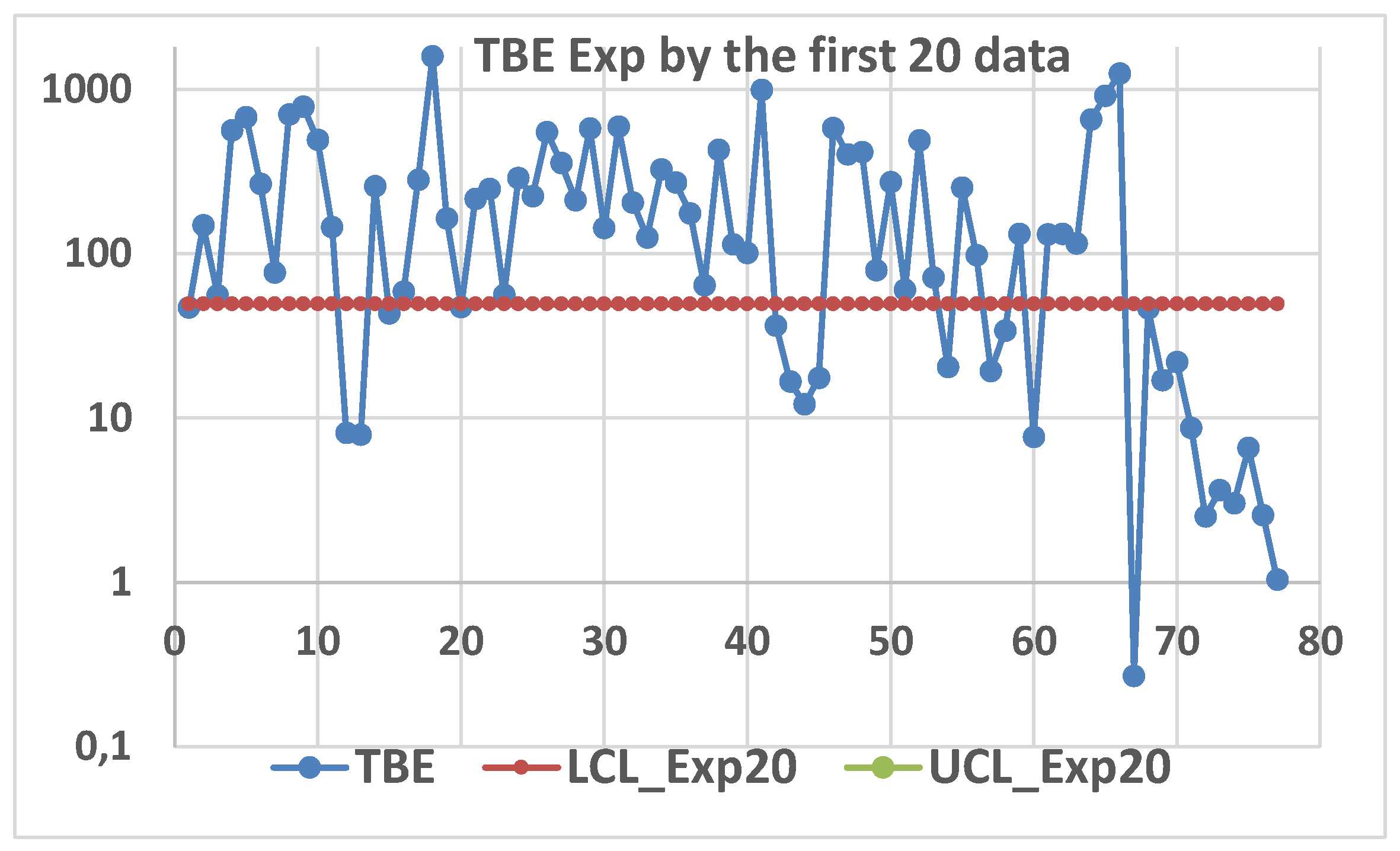
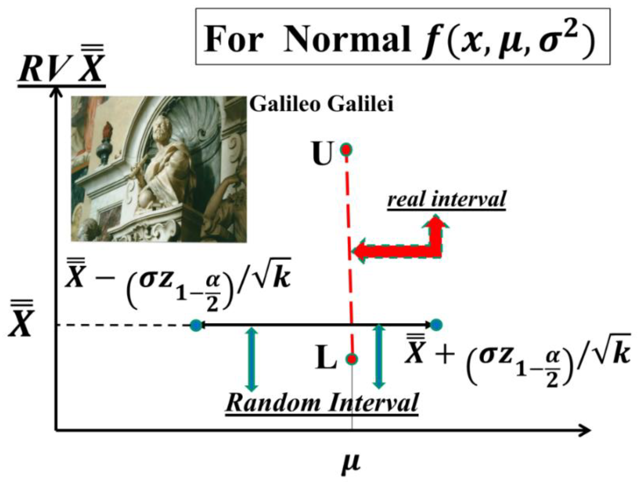
2.1. A Reduced Background of Statistical Concepts
After the ideas given in the Introduction, we provide the following ones essential to understand the “problems related to I-CC” as we found in the literature. We suggest it for the formulae given and for the difference between the concepts of PI (
Probability Interval) and CI (
Confidence Interval): this is overlooked in “
The Garden … [
19]”
Engineering Analysis is related to the investigation of phenomena underlying products and processes; the analyst can communicate with the phenomena only through the observed data, collected with sound experiments (designed for the purpose): any phenomenon, in an experiment, can be considered as a measurement-generating process [MGP, a black box that we do not know] that provides us with information about its behaviour through a measurement process [MP, known and managed by the experimenter], giving us the observed data (the “message”).
It is a law of nature that the data are variable, even in conditions considered fixed, due to many unknown causes.
MGP and MP form the Communication Channel from the phenomenon to the experimenter.
The information, necessarily incomplete, contained in the data, has to be extracted using sound statistical methods (the best possible, if we can). To do that, we consider a statistical model F(x|θ) associated with a random variable (RV) X giving rise to the measurements, the “determinations” D={x1, x2, …, xn} of the RV, constituting the “observed sample” D; n is the sample size. Notice the function F(x|θ) [a function of real numbers, whose form we assume we know] with the symbol θ accounting for an unknown quantity (or some unknown quantities) that we want to estimate (assess) by suitably analysing the sample D.
We indicate by the pdf (probability density function) and by the Cumulative Function, where is the set of the parameters of the functions.
We state in the
Table 2 a sample of models where θ is a set of parameters:
Two important models are the Normal and the Exponential, but we consider also the others for comparison. When
we have the
Normal model, written as
(x|
), with (parameters) mean E[X]=μ and variance Var[X]=σ
2 with pdf
When we have Exponential model, E(x|θ), with (the single parameter) mean E[X]= (variance Var[X]=2), whose pdf is written in two equivalent ways .
When we have the observed sample D={x1, x2, …, xn}, our general problem is to estimate the value of the parameters of the model (representing the parent population) from the information given by the sample. We define some criteria which we require a "good" estimate to satisfy and see whether there exist any "best" estimates. We assume that the parent population is distributed in a form, the model, which is completely determinate but for the value θ0 of some parameter, e.g. unidimensional, θ, or bidimensional θ={μ, σ2}, or θ={β,η,ω}) as in the GIW(x|β,η,ω), or θ={β,η,ω,}) as in the MPGW(x|β,η,ω,.
We seek some function of θ, say τ(θ), named inference function, and we see if we can find a RV T which can have the following properties: unbiasedness, sufficiency, efficiency. Statistical Theory allows us the analysis of these properties of the estimators (RVs).
We use the symbols and for the unbiased estimators T1 and T2 of the mean and the variance.
Luckily, we have that T
1, in the
Exponential model , is efficient [
23,
24,
25,
26,
27,
28,
29,
30,
31,
32,
33,
34,
35,
36,
37,
38,
39,
40,
41,
42,
43,
44,
45,
46,
47,
48,
49,
50,
51,
52,
53,
54], and it extracts the total available information from any random sample, while the couple T
1 and T
2, in the
Normal model, are jointly sufficient statistics for the inference function τ(θ)=(μ, σ
2), so extracting the maximum possible of the total available information from any random sample. The estimators (which are RVs) have their own “distribution” depending on the parent model F(x|θ) and on the sample D: we use the symbol
for that “distribution”. It is used to assess their properties. For a given (collected) sample D the estimator provides a value t (real number) named the
estimate of τ(θ), unidimensional.
A way of finding [
23,
24,
25,
26,
27,
28,
29,
30,
31,
32,
33,
34,
35,
36,
37,
38,
39,
40,
41,
42,
43,
44,
45,
46,
47,
48,
49,
50,
51,
52,
53,
54] the estimate is to compute the
Likelihood Function [LF] and to maximise it: the solution of the equation
=0 is termed
Maximum Likelihood Estimate [MLE]. Both are used also for sequential tests.
The LF is important because it allows us finding the MVB (
Minimum Variance Bound, Cramer-Rao theorem) [
23,
24,
25,
26,
27,
28,
29,
30,
31,
32,
33,
34,
35,
36,
37,
38,
39,
40,
41,
42,
43,
44,
45,
46,
47,
48,
49,
50,
51,
52,
53,
54] of an unbiased RV T [related to the inference function τ(θ)], such that
The inverse of the MVB(T) provides a measure of the total available amount of information in D, relevant to the inference function τ(θ) and to the statistical model F(x|θ).
Naming I
T(T) the information extracted by the RV T we have that [
23,
24,
25,
26,
27,
28,
29,
30,
31,
32,
33,
34,
35,
36,
37,
38,
39,
40,
41,
42,
43,
44,
45,
46,
47,
48,
49,
50,
51,
52,
53,
54]
If T is an Efficient Estimator there is no better estimator able to extract more information from D.
The estimates considered before were “point estimates” with their properties, looking for the “best” single value of the inference function τ(θ).
We recap the very important concept of
Confidence Interval (CI) and Confidence Level (CL) [
23,
24,
25,
26,
27,
28,
29,
30,
31,
32,
33,
34,
35,
36,
37,
38,
39,
40,
41,
42,
43,
44,
45,
46,
47,
48,
49,
50,
51,
52,
53,
54].
The “interval estimates” comprise all the values between τL (Lower confidence limit) and τU (Upper confidence limit); the CI is defined by the numerical interval CI={τL-----τU}, where τL and τU are two quantities computed from the observed sample D: when we make the statement that τ(θ)∈CI, we accept, before any computation, that, doing that, we can be right, in a long run of applications, (1-α)%=CL of the applications, BUT we cannot know IF we are right in the single application (CL=Confidence Level).
We know, before any computation, that we can be wrong α% of the times but we do not know when it happens.
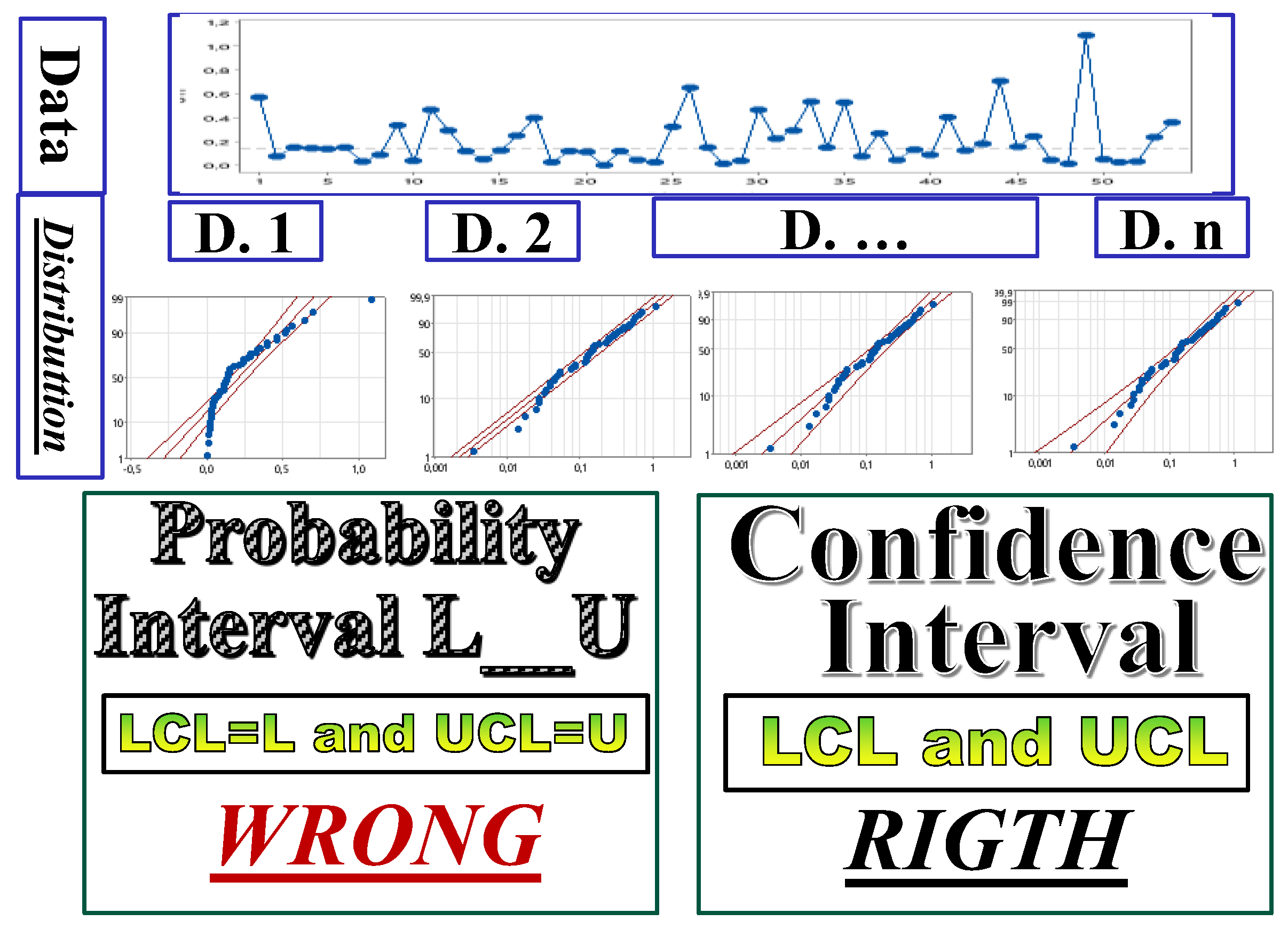
The reader must be very careful to distinguish
between the
Probability Interval PI={L
-----U}, where the endpoints L and U depends on the distribution
of the estimator T (that we decide to use, which
does not depend on the “observed sample” D) and, on the probability π=1-α (that we fix before any computation), as follows by the probabilistic statement (9) [se the
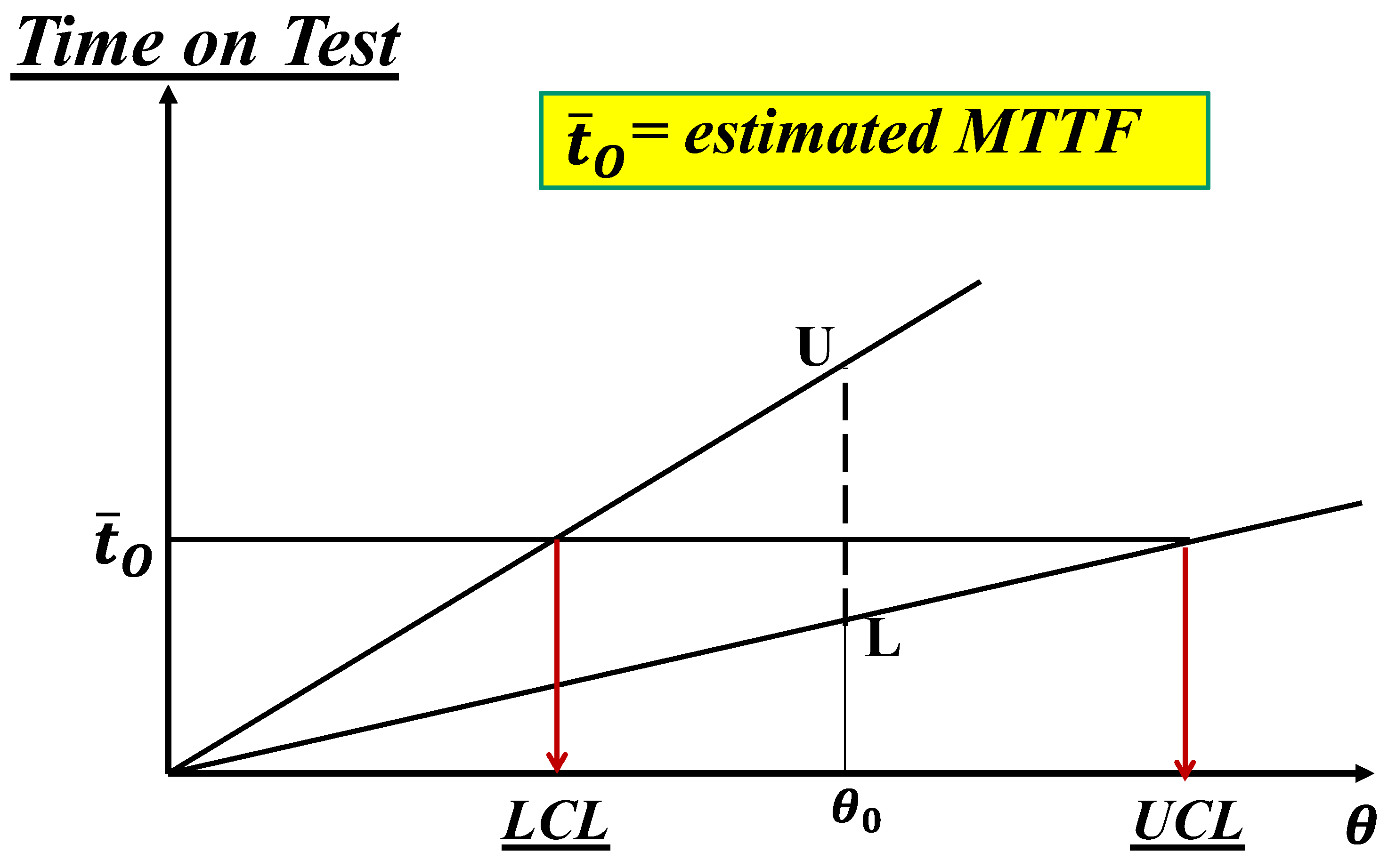
Figure 2 for the exponential density, when n=1]
and the Confidence Interval CI={τL-----τU} which depends on the “observed sample” D.
Notice that the Probability Interval PI={L
-----U}, given in the formula (9),
does not
depend on the data D, as you can pictorially see in
Figure 2: L and U are the Probability Limits. Notice that, on the contrary, the Confidence Interval CI={τ
L-----τ
U}
does depend on the data D, pictorially seen in
Figure 2. This point is essential for all the papers in the References.
Shewhart identified this approach, L and U, on page 275 of [
40] where he states:
| “For the most part, however, we never know [this is the symbols of Shewhart for our ] in sufficient detail to set up such limit… We usually chose a symmetrical range characterised by limits symmetrically spaced in reference to . Tchebycheff’s Theorem tells us that the probability P that an observed value of will lie within these symmetric limits so long as the quality standard is maintained satisfies the inequality P>1-1/t2. We are still faced with the choice of t. Experience indicated that t=3 seems to be an acceptable economic value”. See the excerpts 3,… |
The Tchebycheff Inequality: IF the RV X is arbitrary with density f(x) and finite variance THEN we have the probability , where . This is a “Probabilistic Theorem”.
It can be transferred into
Statistics. Let’s suppose that we want to determine experimentally the unknown mean
within a “stated error ε”. From the above (Probabilistic) Inequality we have
; IF
THEN the event
is “very probable” in an experiment: this means that the observed value
of the RV X can be written as
and hence
. In other words, using
as an estimate of
we commit an error that “most likely” does not exceed
. IF, on the contrary,
, we need n data in order to write
, where
is the RV “mean”; hence we can derive
., where
is the “empirical mean” computed from the data. In other words, using
as an estimate of
we commit an error that “most likely” does not exceed
. See the
Excerpts 3,
3a,
3b.
Notice that, when we write
, we consider the Confidence Interval CI [
23,
24,
25,
26,
27,
28,
29,
30,
31,
32,
33,
34,
35,
36,
37,
38,
39,
40,
41,
42,
43,
44,
45,
46,
47,
48,
49,
50,
51,
52,
53,
54], and no longer the Probability Interval PI [
23,
24,
25,
26,
27,
28,
29,
30,
31,
32,
33,
34,
35,
36,
37,
38,
39,
40,
41,
42,
43,
44,
45,
46,
47,
48,
49,
50,
51,
52,
53,
54].
These statistical concepts are very important for our purpose when we consider the Sequential tests and the Control Charts, especially with Individual data.
Notice that the error made by several authors [
1,
2,
3,
4,
5,
6,
7,
8,
9,
10,
11,
12,
13,
14,
15,
16,
17,
18,
19] is generated by
lack of knowledge of the difference between PI and CI [
23,
24,
25,
26,
27,
28,
29,
30,
31,
32,
33,
34,
35,
36,
37,
38,
39,
40,
41,
42,
43,
44,
45,
46,
47,
48,
49,
50,
51,
52,
53,
54]: they think
wrongly that CI=PI, a diffused disease [
1,
2,
3,
4,
5,
6,
7,
8,
9,
10,
11,
12,
13,
14,
15,
16,
17,
18,
19]! They should study some of the books/papers [
23,
24,
25,
26,
27,
28,
29,
30,
31,
32,
33,
34,
35,
36,
37,
38,
39,
40,
41,
42,
43,
44,
45,
46,
47,
48,
49,
50,
51,
52,
53,
54] and remember the Deming statements (excerpt 2).
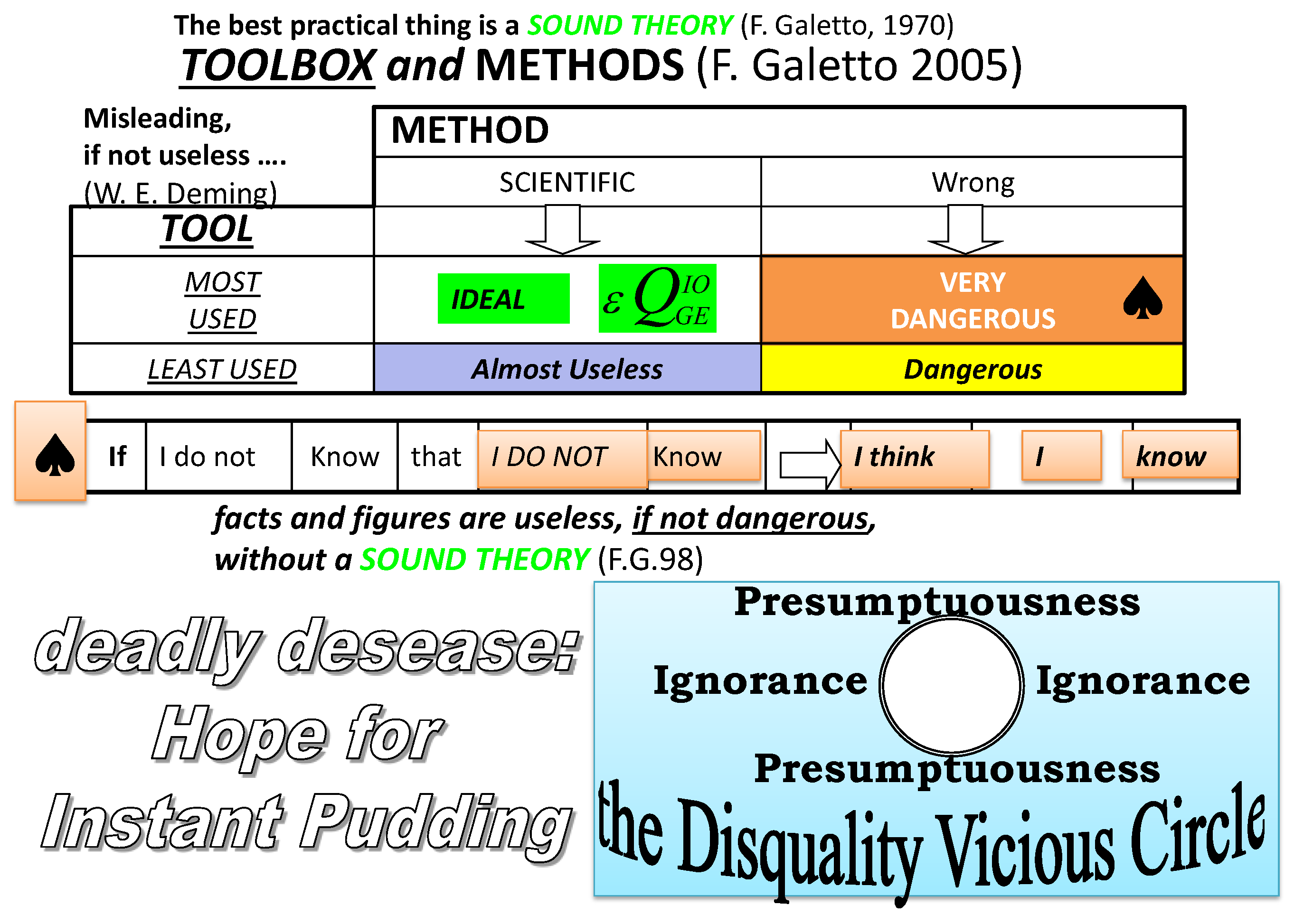
The Deming statements are important for Quality. Managers, scholars; the professors must learn Logic, Design of Experiments and Statistical Thinking to draw good decisions. The authors must, as well. Quality must be their number one objective: they must learn
Quality methods as well, using Intellectual Honesty [
1,
2,
6,
7,
8,
9,
10,
11,
12,
13,
14,
15,
16,
17,
18,
19,
20,
21,
25,
26,
27,
28,
29,
30,
31,
32,
33]. Using (9),
those authors do not
extract the maximum information from the data in the Process Control. To
extract the maximum information from the data one needs statistical valid Methods [
1,
2,
6,
7,
8,
9,
10,
11,
12,
13,
14,
15,
16,
17,
18,
19,
20,
21,
25,
26,
27,
28,
29,
30,
31,
32,
33].
As you can find in any good book or paper [
23,
24,
25,
26,
27,
28,
29,
30,
31,
32,
33,
34,
35,
36,
37,
38,
39,
40,
41,
42,
43,
44,
45,
46,
47,
48,
49,
50,
51,
52,
53,
54] there is a strict relationship between CI and Test Of Hypothesis, known also as Null Hypothesis Significance Testing Procedure (NHSTP). In Hypothesis Testing (see the Introduction), the experimenter wants to assess if a “thought” value of a parameter of a distribution is confirmed (or rejected) by the collected data: for example,
for the mean μ (parameter) of the Normal (x|
) density, he sets the “null hypothesis” H
0={μ=μ
0} and the probability P=α of being wrong if he decides that the “null hypothesis” H
0 is true, when actually it is opposite: H
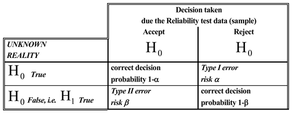
0 is wrong. When we analyse, at once, the
observed sample D={x
1, x
2, …, x
n} and we compute the
empirical (observed)
mean and the
empirical (observed)
standard deviation , we define the
Acceptance interval, which
is the CI
Notice that the interval (for the Normal model,
assumed)
is the Probability Interval such that .
A fundamental reflection is in order: the formulae (10) and (11) tempt the unwise guy to think that he can get the
Acceptance interval, which is
the CI [
23,
24,
25,
26,
27,
28,
29,
30,
31,
32,
33,
34,
35,
36,
37,
38,
39,
40,
41,
42,
43,
44,
45,
46,
47,
48,
49,
50,
51,
52,
53,
54], by substituting the assumed values
of the parameters with the
empirical (observed)
mean and
standard deviation .
This trick is valid only for the Normal distribution.
The formulae (10) can be used sequentially to test H0={μ=μ0} versus H1={μ=μ1<μ0}; for any value 2<k≤n; we obtain n-2 CIs, decreasing in length; we can continue until either μ1<LCL or UCL<μ0, or both (verify) μ1<LCL and UCL<μ0.
More ideas about these points can be found in [
23,
24,
25,
26,
27,
28,
29,
30,
31,
32,
33,
34,
35,
36,
37,
38,
39,
40,
41,
42,
43,
44,
45,
46,
47,
48,
49,
50,
51,
52,
53,
54].
In the field of Control Charts, with Shewhart, instead of the formula (10), we use (12)
where the t distribution value
is replaced by the value
of the Normal distribution, actually
=3, and a coefficient
is used to make “unbiased” the estimate of the standard deviation, computed from the information given by the sample.
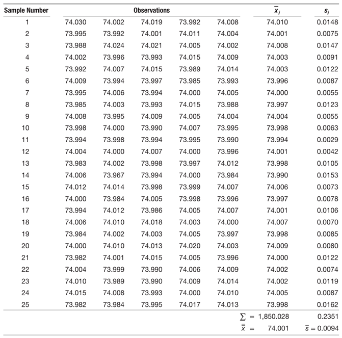
Actually, Shewhart does not use the coefficient is as you can see from page 294 of Shewhart book (1931), where is the “Grand Mean”, computed from D [named here empirical (observed) mean ], is “estimated standard of each sample” (named here s, with sample size n=20, in excerpt 3)
Excerpt 3.
From Shewhart book (1931), on page 294.
Excerpt 3.
From Shewhart book (1931), on page 294.
2.2. Control Limits by AI Versus Sound Theory
In the first part of this section we provide the ideas of the Statistical Theory, while in the second one we see what AI tells us.
Statistical Process Management (SPM) entails Statistical Theory and tools used for monitoring any type of processes, industrial or not. The Control Charts (CCs) are the tool used for monitoring a process, to assess its two states: the first, when the process, named
IC (In Control), operates under the
common causes of variation (variation is always naturally present in any phenomenon) and the second, named
OOC (Out Of Control), when the process operates under some
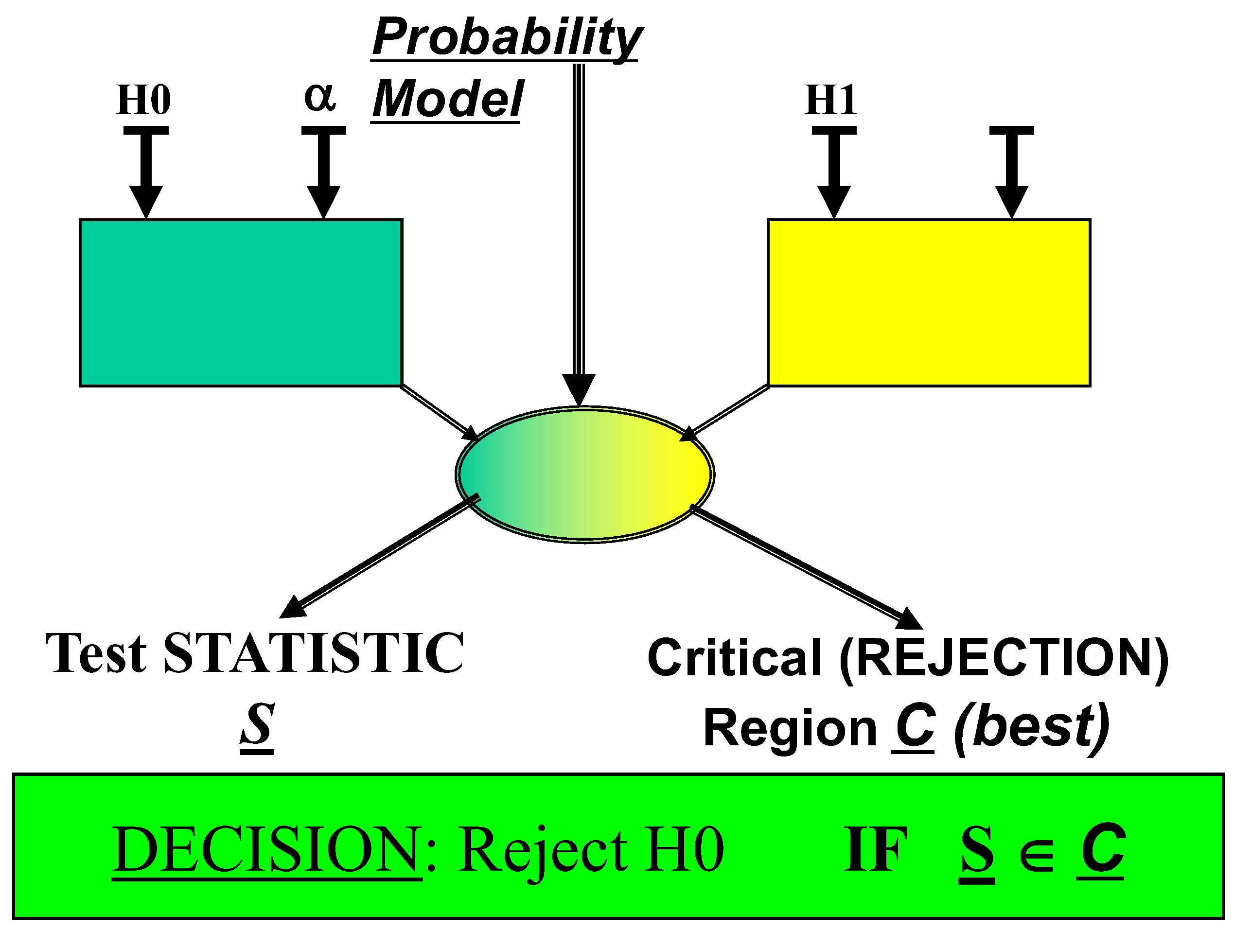
assignable causes of variation. The CCs, using the observed data, allow us to decide if the process is IC or OOC. CCs are a statistical test of hypothesis for the process null hypothesis H
0={IC} versus the alternative hypothesis H
1={OOC}. Control Charts were very considered by Deming [
29,
30] and Juran [
32] after Shewhart invention [
40,
41].
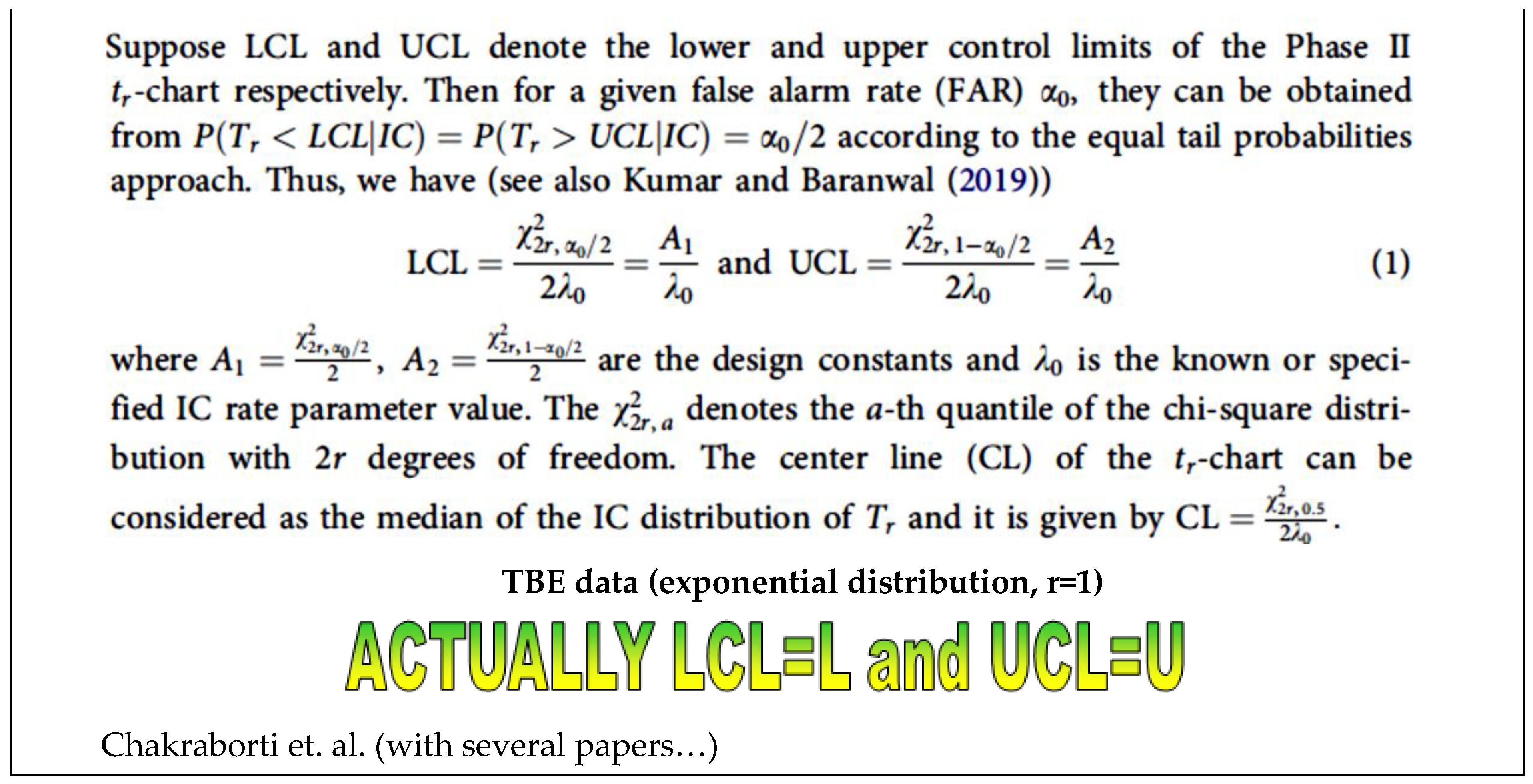
In the excerpts,
is the (experimental) “Grand Mean”, computed from D (we, on the contrary, use the symbol
),
is the (experimental) “estimated standard of each sample” (we, on the contrary, use the symbol s, with sample size n=20, in
Excerpts 3a,
3b),
is the “estimated mean standard deviation of all the samples” (we, on the contrary, use the symbol
).
Excerpt 3a.
From Shewhart book (1931), on page 89.
Excerpt 3a.
From Shewhart book (1931), on page 89.
On page 95, he also states that
Excerpt 3b.
From Shewhart book (1931), on page 294.
Excerpt 3b.
From Shewhart book (1931), on page 294.
So, we clearly see that Shewhart, the inventor of the CCs,
used the data to compute the Control Limits, LCL (Lower Control Limit, which is the Lower
Confidence Limit) and UCL (Upper Control Limit, the Upper
Confidence Limit) both for the mean
(1
st parameter of the Normal pdf) and for
(2
nd parameter of the Normal pdf). They are considered the limits comprising 0.9973n of the observed data. Similar ideas can be found in [
23,
24,
25,
26,
27,
28,
29,
30,
31,
32,
33,
34,
35,
36,
37,
38,
39,
40,
41,
42,
43,
44,
45,
46,
47,
48,
49,
50,
51,
52,
53,
54] (with Rozanov, 1975, we see the idea that CCs can be viewed as a Stochastic Process).
We invite the readers to consider that if one assumes that the process is In Control (IC) and if he knows the parameters of the distribution he can test if the assumed known values of the parameters are confirmed or disproved by the data, then he does not need the Shewhart Control Charts; it is sufficient to use NHSTP or the Sequential Test Theory!
Remember the ideas in the previous section and compare
Excerpts 3,
3a,
3b (where
LCL, UCL depend on the data) with the following
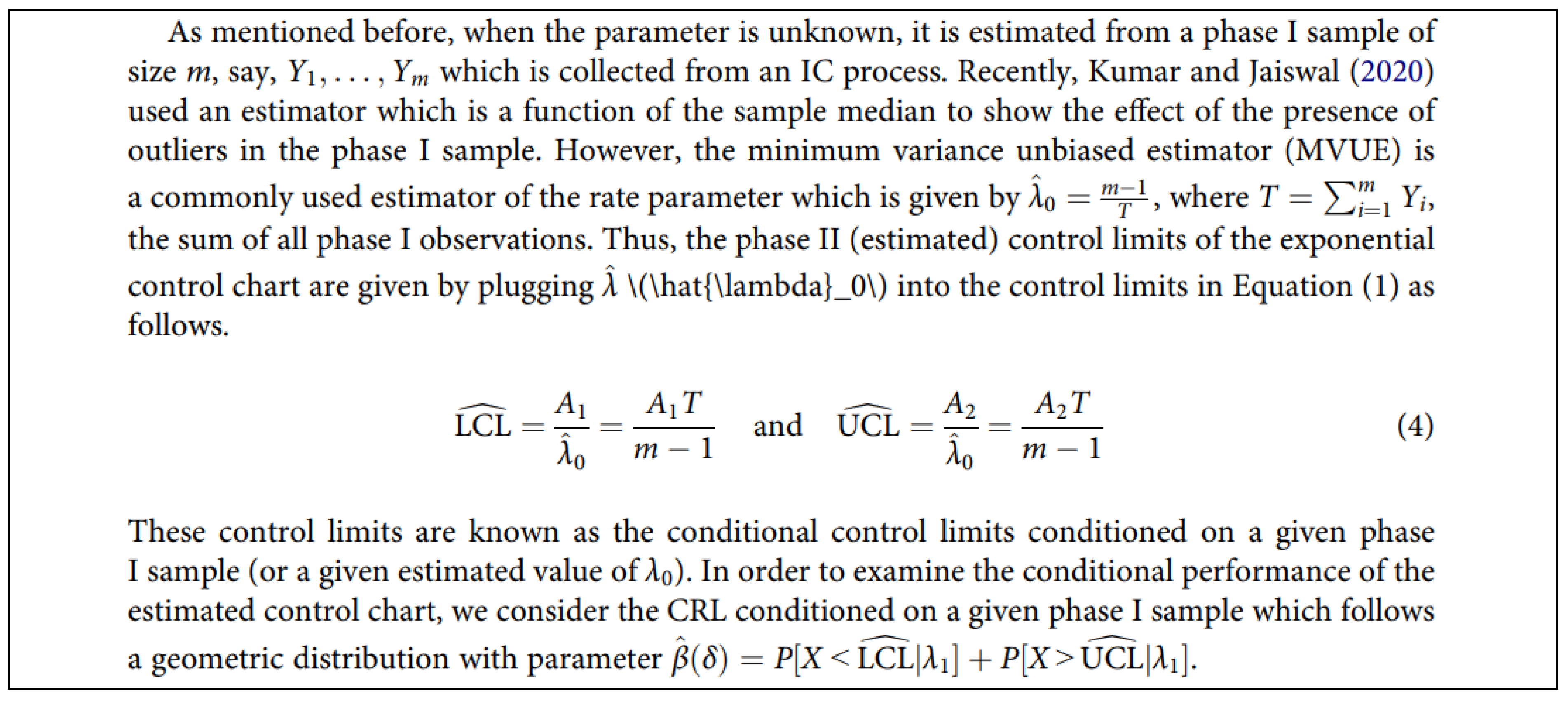
Excerpt 4 (where
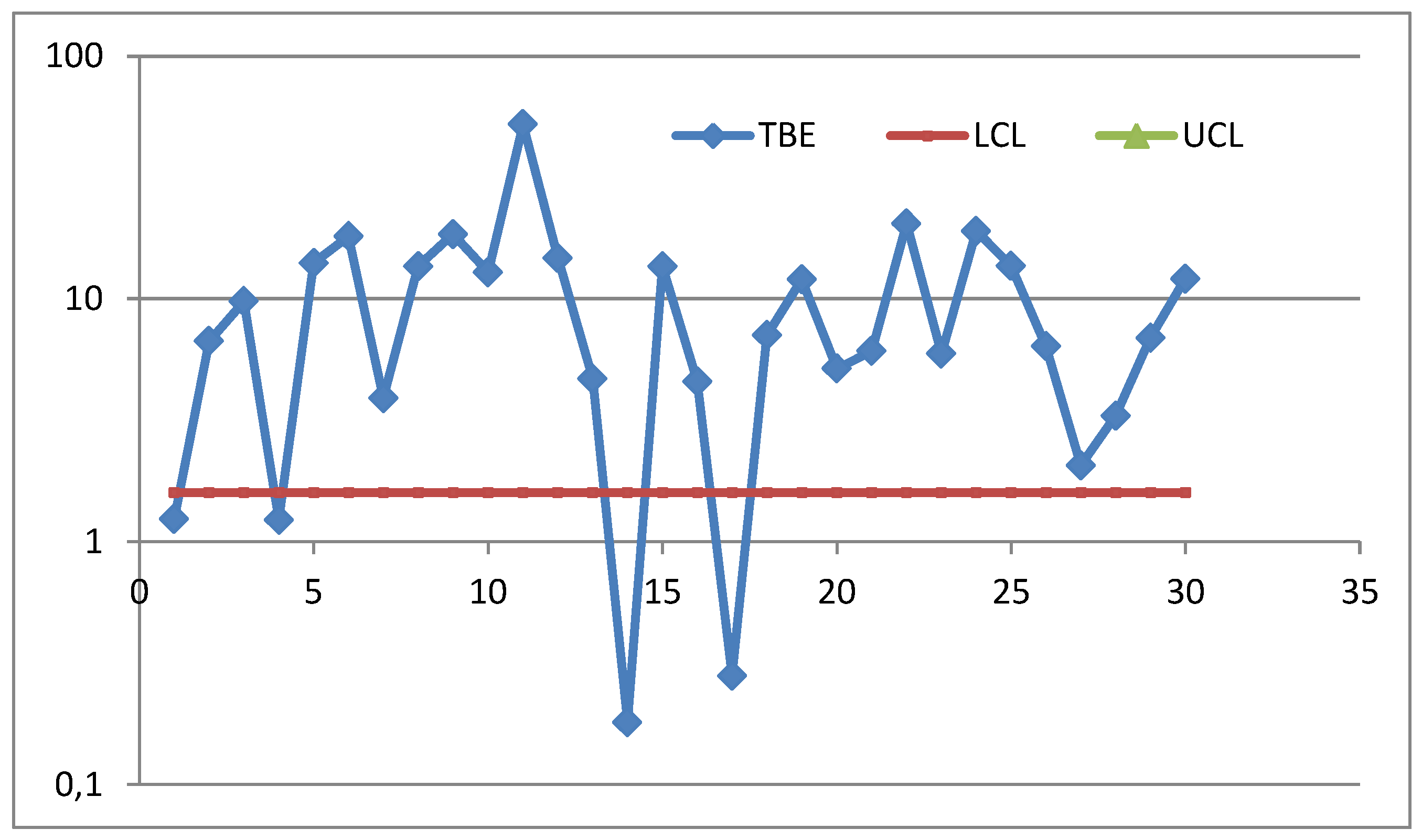
LCL, UCL depend on the Random Variables) and appreciate the profound “logic” difference: this is the cause of the many errors in the CCs for TBE [Time Between Events (see [
19,
42,
43,
44,
45,
46,
47,
48,
49,
50,
51,
52,
53,
54]).
The formulae, in the excerpt 4, LCL
1 and UCL
1 are
actually the
Probability Limits (
L and U) of the
Probability Interval PI in the formula (9), when
is the pdf of the Estimator T, related to the Normal model F(x; μ, σ
2). Using (9),
those authors do not extract the maximum information from the data in the Process Control. From the Theory [
6,
7,
8,
9,
10,
11,
12,
13,
14,
15,
16,
17,
18,
19,
20,
21,
22,
23,
24,
25,
26,
27,
28,
29,
30,
31,
32,
33,
34,
35,
36] we derive that the interval L=
μY-3σY------μY+3
σY=U is the PI such that the RV Y=
and it is not the CI of the mean
μ=
μY [as wrongly said in the
Excerpt 4, where actually (LCL
1-----UCL
1)=PI].
The same error is in other books and papers (not shown here but the reader can see in [
19,
20,
21,
22,
23]).
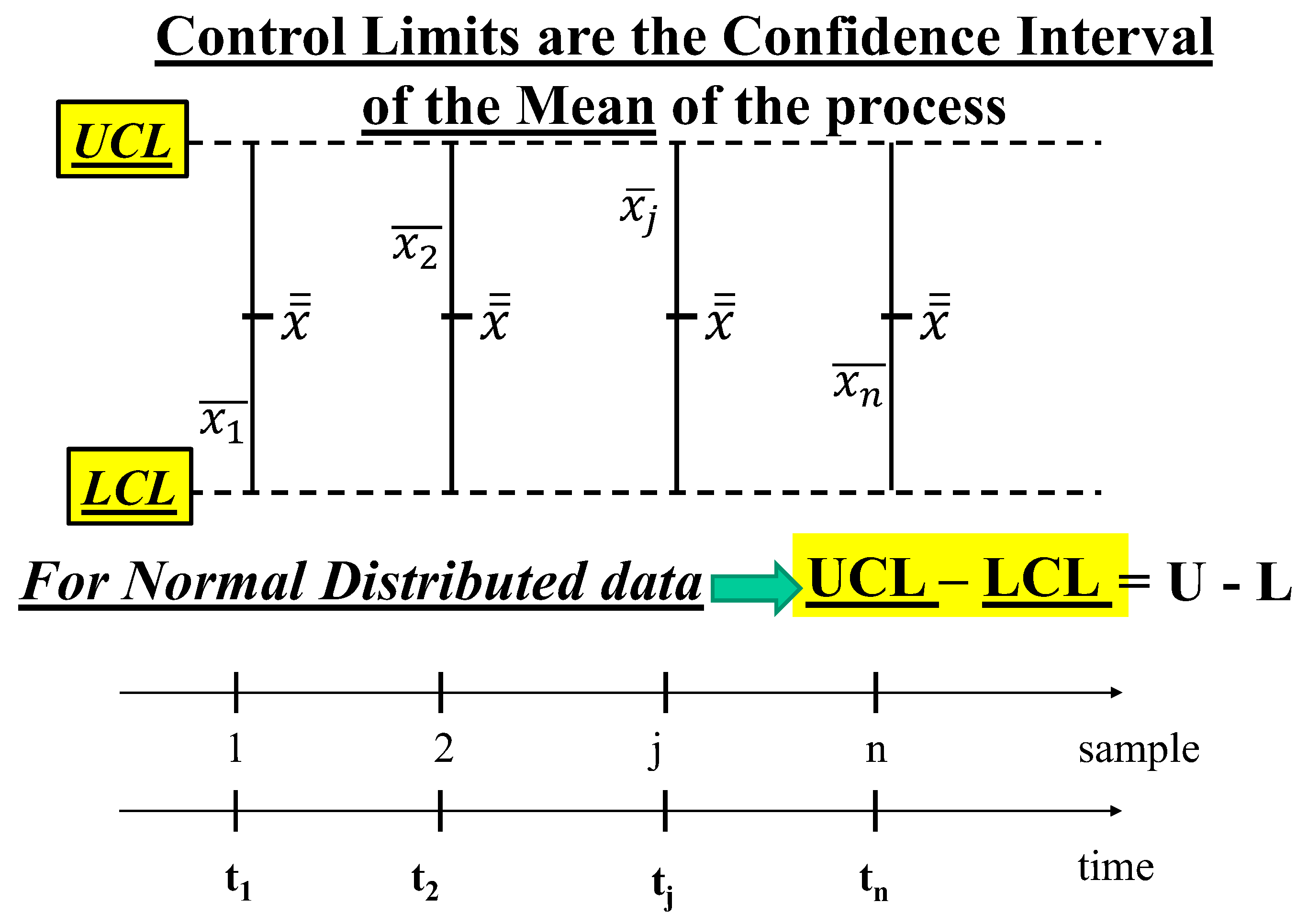
Figure 3.
Control Limits LCLX----UCLX=L----U (Probability interval), for Normal data (Individuals xij, sample size k) “sample means” and “grand mean”
Figure 3.
Control Limits LCLX----UCLX=L----U (Probability interval), for Normal data (Individuals xij, sample size k) “sample means” and “grand mean”
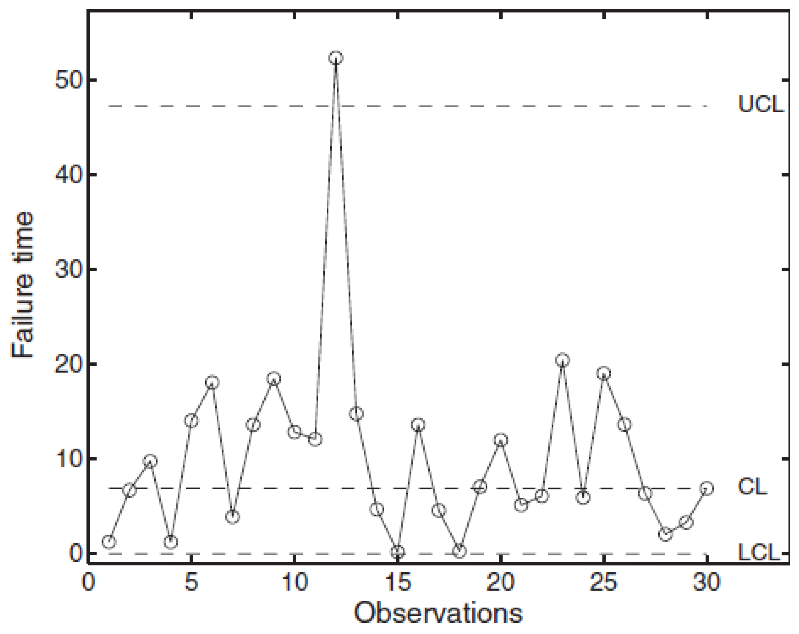
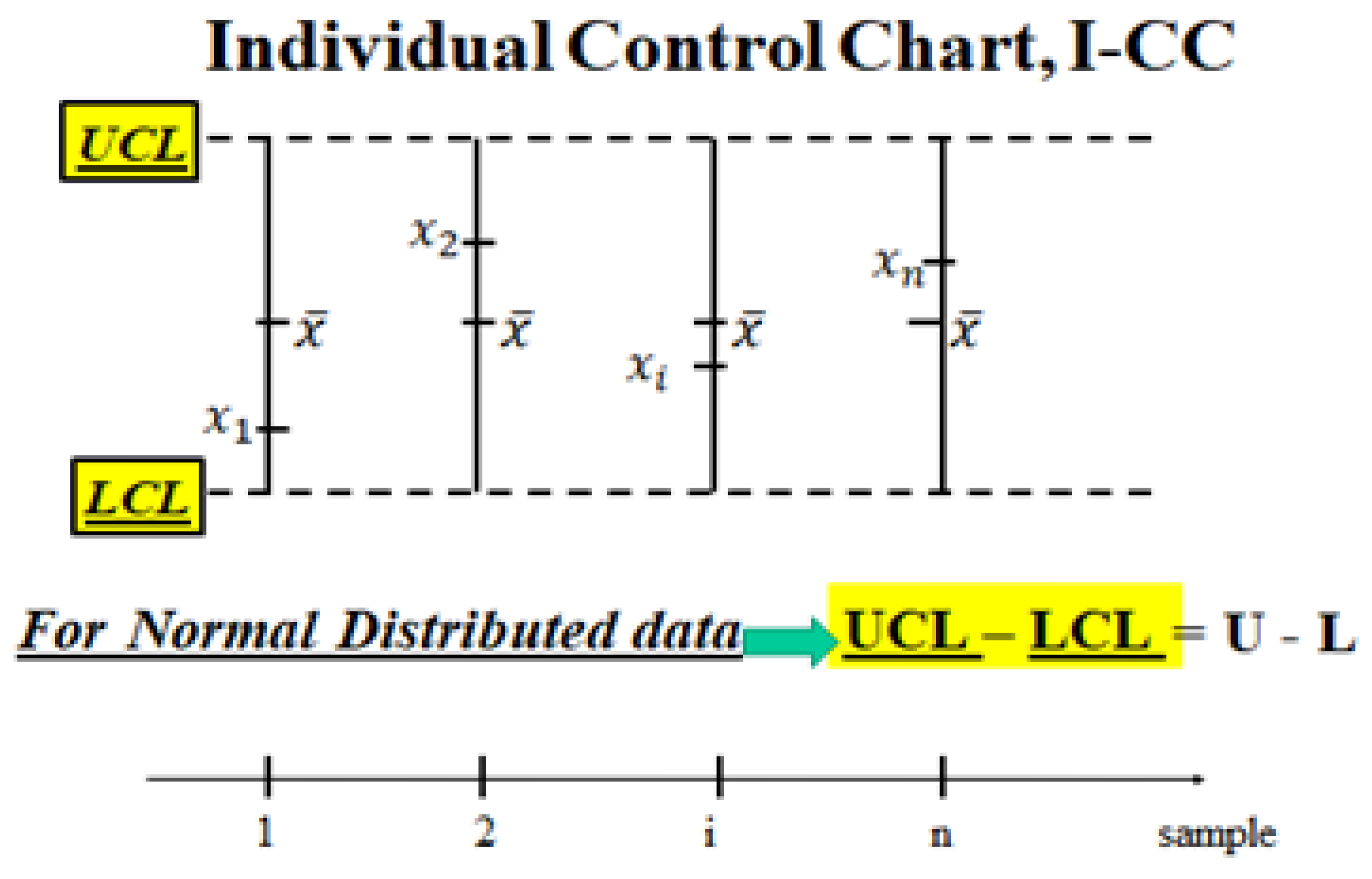
Figure 4.
Individual Control Chart (sample size k=1). Control Limits LCL----UCL=L----U (Probability interval), for Normal data (Individuals xi) and “grand mean”
Figure 4.
Individual Control Chart (sample size k=1). Control Limits LCL----UCL=L----U (Probability interval), for Normal data (Individuals xi) and “grand mean”
The data plotted in the CCs [
23,
24,
25,
26,
27,
28,
29,
30,
31,
32,
33,
34,
35,
36,
37,
38,
39,
40,
41,
42,
43,
44,
45,
46,
47,
48,
49,
50,
51,
52,
53,
54] (see the
Figure 3-
4) are the means
, determinations of the RVs
, i=1, 2, ..., n (n=number of the samples) computed from the
sequentially collected data of the i-th sample D
i={x
ij, j=1, 2, ..., k} (k=sample size)}, determinations of the RVs
at
very close instants t
ij, j=1, 2, ..., k. In other applications I-CC (see the
Figure 3), the data plotted are the Individual Data
, determinations of the Individual Random Variables
, i=1, 2, ..., n (n=number of the collected data), modelling the measurement process (MP) of the “Quality Characteristic” of the product: this model is very general because it is able to consider every distribution of the Random Process
, as we can see in the next section. From the
Excerpts 3,
3a,
3b and formula (10) it is clear that Shewhart was using the Normal distribution, as a consequence of the
Central Limit Theorem (CLT) [
23,
24,
25,
26,
27,
28,
29,
30,
31,
32,
33,
34,
35,
36,
37,
38,
39,
40,
41,
42,
43,
44,
45,
46,
47,
48,
49,
50,
51,
52,
53,
54]. In fact, he wrote on page 289 of his book (1931) “
… we saw that, no matter what the nature of the distribution function of the quality is, the distribution of the arithmetic mean approaches normality rapidly with increase in n (
his n is our k)
, and in all cases the expected value of means of samples of n (our k)
is the same as the expected value of the universe” (CLT in
Excerpt 3,
3a,
3b).
Let k be the sample size; the RVs are assumed to follow a normal distribution and uncorrelated; [ith rational subgroup] is the mean of RVs IID j=1, 2, ..., k, (k data sampled, at very near times tij).
To show our way of dealing with CCs we consider the process as a “
stand-by system whose transition times from a state to the subsequent one” are the collected data. The lifetime of “stand-by system” is the sum of the lifetimes of each unit. The process (modelled by a “stand-by …”) behaves as a Stochastic Process
[
25,
26,
27,
28,
29,
30,
31,
32,
33], that we can manage by the Reliability Integral Theory (RIT): see the next section; this method is very general because it is able to consider every distribution of
.
If we assume that
is distributed as f(x) [probability density function (pdf) of “transitions from a state to the subsequent state” of a stand-by subsystem] the pdf of the (RV) mean
is, due the CLT (page 289 of 1931 Shewhart book),
[experimental mean
] with mean
and variance
.
is the “grand” mean and
is the “grand” variance: the pdf of the (RV) grand mean
[experimental “grand” mean
]. In
Figure 2 we show the determinations of the RVs
and of
.
When the process is Out Of Control (OOC,
assignable causes of variation, some of the means
, estimated by the experimental means
, are “statistically different)” from the others [
23,
24,
25,
26,
27,
28,
29,
30,
31,
32,
33,
34,
35,
36,
37,
38,
39,
40,
41,
42,
43,
44,
45,
46,
47,
48,
49,
50,
51,
52,
53,
54]. We can assess the OOC state of the process via the Confidence Intervals (by the Control Limits) with CL=0.9973.
Remember the
trick valid only for the Normal Distribution ….; consider the PI,
L=
μY-3
σY------μY+3
σY=
U; putting
in place of
and
in place of
we get the CI of
when the sample size k is considered for each
, with CL=0.9973. The quantity
is the mean of the standard deviations of each sample. This allows us to compare each (subsystem) mean
, q=1,2, …, n, to any other (subsystem) mean
r=1,2, …, n, and to the (Stand-by system) grand mean
. If two of them are different, the process is classified as OOC. The quantities
and
are the Control Limits of the CC, which are the
Confidence Limits. When the Ranges R
i=max(x
ij)-min(x
ij) are considered for each sample we have
,
and
, U
, where
is the “mean range” and the coefficients A
2, D
3, D
4 are tabulated and depend on the sample size k [
23,
24,
25,
26,
27,
28,
29,
30,
31,
32,
33,
34,
35,
36,
37,
38,
39,
40,
41,
42,
43,
44,
45,
46,
47,
48,
49,
50,
51,
52,
53,
54].
We stress that the interval LCL
X-------UCL
X is the “
Confidence Interval” with “Confidence Level” CL=1-α=0.9973 for the unknown mean
of the Stochastic Process X(t) [
23,
24,
25,
26,
27,
28,
29,
30,
31,
32,
33,
34,
35,
36,
37,
38,
39,
40,
41,
42,
43,
44,
45,
46,
47,
48,
49,
50,
51,
52,
53,
54]. The interval LCL
R----------UCL
R is the “Confidence Interval” with “Confidence Level” CL=1-α=0.9973 for the unknown Range of the Stochastic Process X(t) [
23,
24,
25,
26,
27,
28,
29,
30,
31,
32,
33,
34,
35,
36,
37,
38,
39,
40,
41,
42,
43,
44,
45,
46,
47,
48,
49,
50,
51,
52,
53,
54].
Notice that, ONLY for normally distributed data, the length of the Control Interval (UCLX-LCLX, which is the Confidence Interval) equals the length of the Probability Interval, PI (U-L): UCLX-LCLX=U-L.
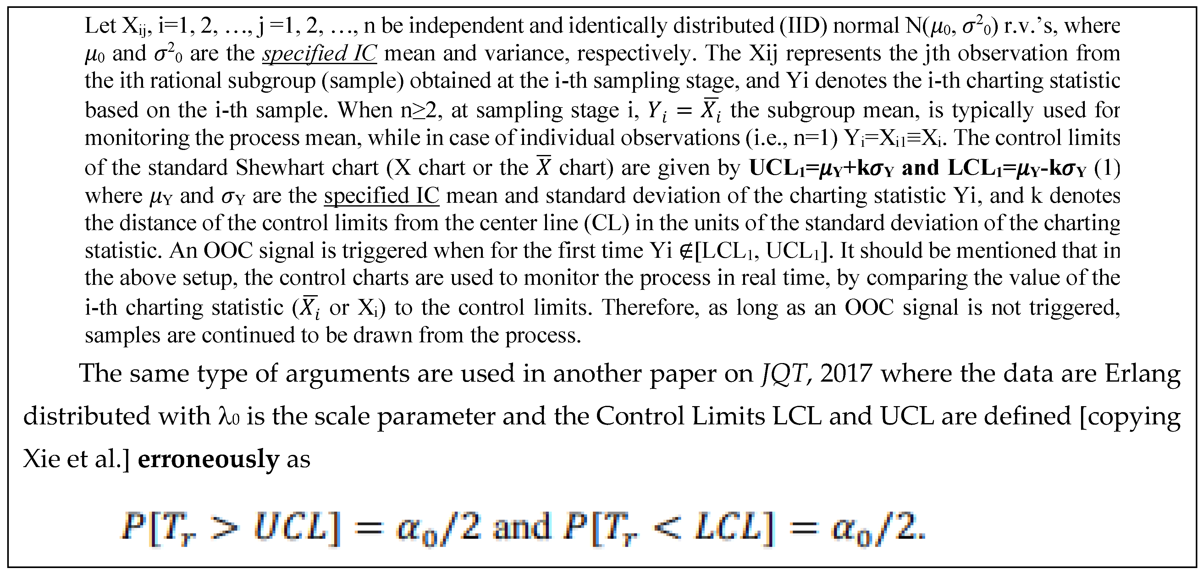
The error highlighted, i.e. the
confusion between the Probability Interval and the Control Limits (Confidence Interval!) has
no consequences for decisions
when the data are
Normally distributed, as considered by Shewhart. On the contrary, it has BIG consequences for decisions
WHEN the data are Non-Normally distributed [
23,
24,
25,
26,
27,
28,
29,
30,
31,
32,
33,
34,
35,
36,
37,
38,
39,
40,
41,
42,
43,
44,
45,
46,
47,
48,
49,
50,
51,
52,
53,
54,
55,
56,
57,
58,
59,
60,
61,
62,
63,
64,
65,
66,
67,
68,
69,
70,
71,
72,
73,
74].
We think that the paper “Quality of Methods for Quality is important”, [
24] appreciated and mentioned by J. Juran at the plenary session of the EOQC (European Organization for Quality Control) Conference (1989), should be considered and meditated.
| ====== Now we see what AI answered to our queries.====== |
First Query: [NOTICE that the answer is like from the Theory!]
How can I compute LCL and UCL in Control Charts for individuals Normally distributed?
ChatGPT says:
To compute the Lower Control Limit (LCL) and Upper Control Limit (UCL) in Control Charts for Individuals (also called Individuals or X Charts), especially when the data is normally distributed, follow this step-by-step process:


1. Understanding Control Charts for Individuals
When you're dealing with individual measurements (i.e. sample size = 1), you usually use:
You don't have subgroups like in X-bar and R charts — you're monitoring single data points.


2. Basic Definitions
: Mean of individual measurements
MR: Moving range (difference between consecutive individual values)
: Average of the moving ranges
d2: A constant depending on subgroup size (for n=2, d2≈1.128)


3. Formulae for Control Limits

Individuals (X) Chart:
To estimate the process standard deviation:
Then: Center Line (CL): , UCL: +3, LCL: -3
Substitute for : UCL= +3, LCL= -3

Moving Range (MR) Chart: CL:
, UCL: D4⋅
, LCL: D3⋅
For moving range of 2 (i.e., MR = |Xᵢ − Xᵢ₋₁|): D4=3.267, D3=0


4. Step-by-Step Example
Suppose you have this data: X=[10,12,11,13,12]
Step 1: Compute , =(10+12+11+13+12)/5
Step 2: Compute Moving Ranges, MR={∣12−10∣,∣11−12∣,∣13−11∣,∣12−13∣}=[2,1,2,1] =(2+1+2+1)/4=1.5
Step 3: Estimate standard deviation =1.5/1.128≈1.33
Step 4: Compute Control Limits
So your X Chart limits are: UCL = 15.59, CL = 11.6, LCL = 7.61


Summary of Constants for n = 2:
| Constant |
Value |
| d2 |
1.128 |
| D3 |
0 |
| D4 |
3.267 |

Notes
This method assumes normality of the data and independence of observations.
If there is autocorrelation, the control chart may not work well.
Avoid using standard deviation directly unless the population SD is known.
Second Query: [NOTICE that the answers are all wrong!]
How can I compute LCL and UCL in Control Charts for individuals Exponentially distributed?
ChatGPT says:
To compute the Lower Control Limit (LCL) and Upper Control Limit (UCL) for individual control charts (I-Charts) when the data follow an exponential distribution, you need to take into account that the usual assumptions for I-Charts (normality, constant variance, etc.) do not hold. However, there are appropriate methods adapted for exponential data.


Overview of the Problem
You have individual observations (i.e., no subgroups).
The data follow an Exponential distribution (e.g., lifetimes, waiting times).
Traditional I-chart (X chart) limits assuming normality may not be appropriate

Approach to Control Charts for Exponentially Distributed Data
The exponential distribution is often used to model the time between events in a Poisson process. It has a probability density function (PDF) given by: f(x∣λ)=λe−λx,x≥0 where λ is the rate parameter, which is the inverse of the mean (i.e., λ=1/μ.
The exponential distribution is not symmetric (it's positively skewed), and has:
Control Charts for Individual Measurements:
For individual measurements from an exponential distribution, you can use Shewhart control charts adapted for exponential data, typically using a transformation or using a non-normal chart like the exponential control chart.
UCL and LCL Formula:
For an exponentially distributed process, the formulas for the UCL and LCL are typically derived from the properties of the exponential distribution.
Center Line (CL): The center line is the expected value (mean) of the exponentially distributed data, i.e., μ.
UCL and LCL are typically calculated as a function of the standard deviation (or sometimes the range) of the individual data points and a constant multiplier (commonly denoted as -3 +3 for a 3-sigma control chart).
Steps to Calculate:
For an exponentially distributed process, the standard deviation of the individual data points is also μ, which is the same as the mean (since for an exponential distribution, the mean and standard deviation are equal); UCL (Upper Control Limit): UCL=μ+3μ=4μ and LCL (Lower Control Limit): LCL=μ−3μ=−2μ
However, since you can't have negative values for exponentially distributed data (because the data cannot go below zero), if the LCL becomes negative, it should be set to 0.
Therefore, the LCL is: LCL=max[0, −2μ]
- 3.
Plotting the Control Chart:
Once you have the UCL, LCL, and mean, you can plot the individual data points and compare them against the control limits. The control chart will signal out-of-control points when they fall outside the UCL or LCL.
Example: Suppose you have the following data points from an exponentially distributed process: 2.1, 3.0, 1.8, 2.5, 3.3, 2.9
Calculate the mean: μ=(2.1+3.0+1.8+2.5+3.3+2.9)/6=2.67
-
Calculate the UCL and LCL:
- ○
UCL: UCL=4x2.67=10.68, LCL:LCL=max (0,−4.01)=0
So, for this dataset, the UCL is 10.68 and the LCL is 0.
This is the basic process for computing control limits for individual exponentially distributed data in a control chart. Would you like to go over an example in more detail or dive into other aspects of control charts?
◇ Method 1: Control Chart Using Transformation (Log Transformation)
You can transform exponential data to approximate normality:
Let Xi∼Exponential(λ)
Then Yi=ln(Xi) is approximately Gumbel distributed, which may still not be normal, but may behave better.
Construct the chart based on Yi, then back-transform control limits if needed.
However, this is approximate and not always reliable.
◇ Method 2: Use of Quantiles – Exact Method for Exponential
Since exponential data is skewed, control limits can be set using quantiles of the exponential distribution. Given:
Then the LCL and UCL are set using percentiles from the exponential distribution:

Control Limits for Individuals (based on quantiles):
If you want to set the control limits at, say, 3-sigma equivalent (which covers ~99.73% of normal data), then instead of standard deviation, use percentiles:
Let’s say your exponential distribution has rate λ, i.e. X∼Exp(λ), with mean μ=1/λ.
Then: LCL = [F(α/2)=]{-1}=−(1/λ)ln(1−α/2) and UCL = [F1-(α/2)=]{-1}=−(1/λ)ln(α/2)
For example, if you want the control limits to cover 99.73% (like ±3σ in normal distribution), set α=1−0.9973=0.0027
So: LCL = −(1/λ)ln(1−0.00135) and UCL = −(1/λ)ln(0.00135)
This gives you asymmetric control limits appropriate for exponential data.

◇ Method 3: Use of Moving Range (I-MR Chart Alternative)
If you still want to use the Individuals-Moving Range (I-MR) chart:
Use mean of individual observations as the center line.
Estimate the average moving range
Estimate process standard deviation: , where d2≈1.128 for moving range of 2.
Then control limits: UCL=+3, and LCL=-3

Caution: This assumes approximate normality, which does not hold for exponential data. Thus, this is not strictly valid unless the exponential is close to symmetric (i.e., large mean).


Recommended: Use Exponential Distribution Quantiles (Method 2)
If you’re confident the process follows an exponential distribution (e.g., lifetimes, waiting times, times between failures), the quantile-based control limits (Method 2) are the most appropriate.

Example: Assume λ=0.5, so μ=2
Using α=0.0027, LCL≈−2ln(0.99865)≈0.0027, and UCL=−2ln(0.00135)≈13.21
So, your control limits would be: CL = 2, LCL ≈ 0.0027, UCL ≈ 13.21

Summary
| Method |
Use when |
Notes |
| Transformation |
Data not too skewed |
Approximate, may not always help |
| Quantiles (recommended) |
Exponential model is appropriate |
Exact, statistically valid |
| I-MR Chart |
Simpler method needed |
Assumes normality; use with caution |
If you'd like, I can help generate control limits for your actual data or simulate an example. Just upload your dataset or specify the λ (or sample of data).
Third Query: [NOTICE that the answers are all wrong!]
How can I compute LCL and UCL in Control Charts for individuals Exponentially distributed?
ChatGPT says:
To compute the Lower Control Limit (LCL) and Upper Control Limit (UCL) for Control Charts for individuals when the data is exponentially distributed, we need to acknowledge that:
The exponential distribution is not symmetric, unlike the normal distribution assumed in traditional Shewhart Individuals (I) charts.
Standard I-MR (Individuals and Moving Range) charts assume normality, so applying them directly to exponential data can lead to incorrect control limits.
However, with appropriate transformation or modified control limits, you can still monitor such processes.

Option 1: Transform the data to normality
If your data X∼Exponential(λ), then:
However, since control charts often require normality, it's common to apply log transformation and then use regular Individuals charts on the transformed data. Here's how:

Steps for Log-Transformed I-chart:
□ 2 Compute:
□ 3 Estimate the standard deviation using:
□ 4 Compute UCL and LCL for the I-chart of logged data:
□ 5 To get control limits in the original scale, exponentiate the limits:
This approach makes the data approximately normal, so standard control chart techniques become valid.

Option 2: Use control charts designed for exponential data
Some practitioners and researchers propose specialized control charts for exponential distributions, like:
1. Exponential EWMA (Exponentially Weighted Moving Average)
2. Cumulative Sum (CUSUM) control charts
3. Exact UCL/LCL for exponential data
If you insist on not transforming the data, here's a rough approximation based on percentiles: Let X∼Exponential(λ), then: Mean: μ=1/λ, Standard deviation: σ=1/λ
If you approximate 3-sigma limits like a normal distribution (though not ideal), then:
But LCL would be negative, which is not possible for exponential data (since it's strictly positive). So we either:
Set LCL = 0 (common in some practices), or
Use percentile-based control limits, like:
where F
−1 is the inverse CDF of the exponential distribution, and p1, p2 are lower and upper percentiles (e.g., 0.0015 and 0.9985 for 3-sigma equivalent).

Recommended Approach
Use the log-transformed individuals chart, which works well in practice and maintains simplicity. Here's a summary:
| Step |
Action |
| 1 |
Take Yi=ln(Xi) |
| 2 |
Compute , MRi , and |
| 3 |
Estimate |
| 4 |
Get UCL and LCL in log scale:
|
| 5 |
Exponentiate limits:
|
Let me know if you'd like a worked example or Excel template for this.
| ====== End of answers of AI to our queries.====== |
NOTICE that the AI answers are wrong for Exponentially distributed data: AI is actually AIG (Artificial IGnorance).
The following section explains why.
2.3. Statistics and Reliability Integral Theory (RIT)
We are going to present the fundamental concepts about RIT (Reliability Integral Theory) that we use for computing the Control Limits (
Confidence Limits) of CCs. RIT is the natural way for Sequential Tests, because the transitions happen
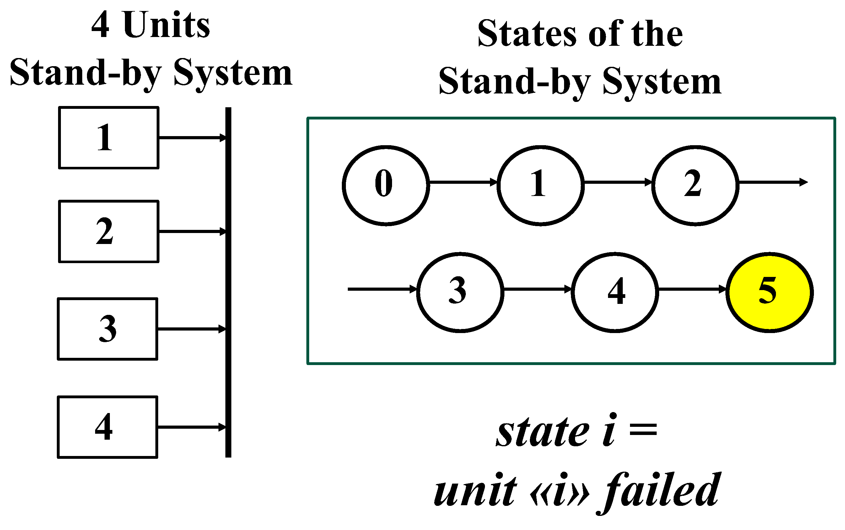
sequentially; to provide the ideas, we use a “4 units Stand-by system”, depicted by 5 states (
Figure 5): 0 is the state with all units not-failed; 1 is the state with the first unit failed; 2 is the state with the second unit failed; and so on, until the system enters the state 5 where all the 4 units are failed (down state, in yellow): any transition provides a datum to be used for the computations. RIT can be found in the author’s books…
RIT can be used for parameters estimation and Confidence Intervals (CI), (Galetto 1981, 1982, 1995, 2010, 2015, 2016), in particular for Control Charts (Deming, 1986, 1997, Shewhart 1931, 1936, Galetto 2004, 2006, 2015). In fact, any Statistical or Reliability Test can be depicted by an “Associated Stand-by System” [
25,
26,
27,
28,
29,
30,
31,
32,
33,
34,
35,
36] whose transitions are ruled by the kernels b
k,j(s); we write the
fundamental system of integral equations for the reliability tests, whose duration t is related to interval 0
-----t; the collected data t
j can be viewed as the times of the various failures (of the units comprising the System) [t
0=0 is the start of the test, t is the end of the test and g is the number of the data (4 in the
Figure 5)]
Firstly, we assume that the kernel
is the pdf of the exponential distribution
(
|
)
, where
is the failure rate of each unit and
:
is the MTTF of each unit. We state that
is the probability that the stand-by system does not enter the state g (5 in
Figure 5), at time t, when it starts in the state j (0, 1, …, 4) at time t
j,
is the probability that the system does not leave the state j,
is the probability that the system makes the transition j→j+1, in the interval s
-----s+ds.
The system reliability
is the solution of the mathematical system of the Integral Equations (13)
With
we obtain the solution (see
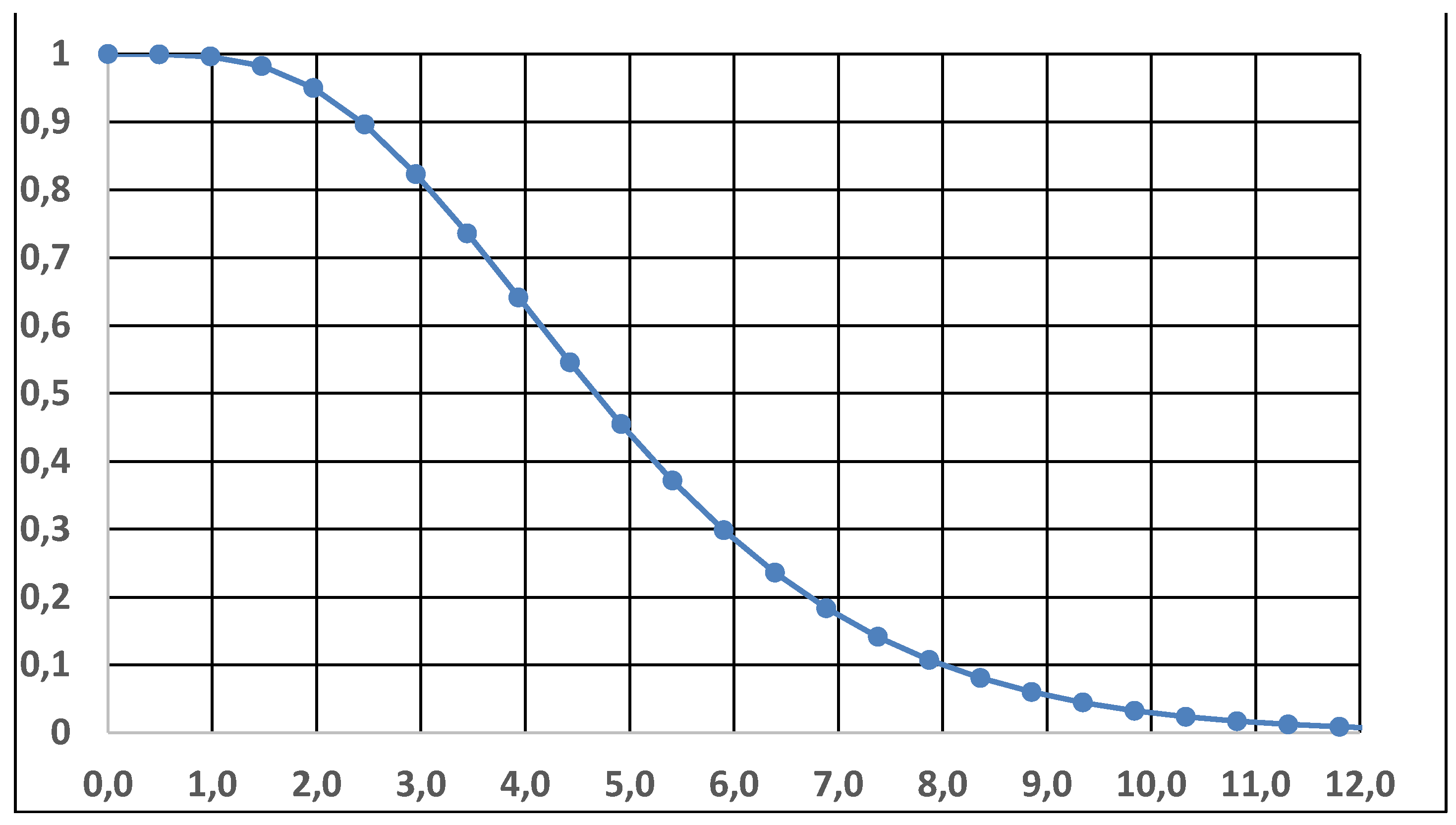
Figure 5, putting the Mean Time To Failure MTTF of each unit=θ,
) (see the
Figure 6)
The reliability system (13) can be written in matrix form,
At the end of the reliability test, at time t, we know the data (the times of the transitions tj) and the “observed” empirical sample D={x1, x2, …, xg}, where xj=tj – tj-1 is the length between the transitions; the transition instants are tj = tj-1 + xj giving the “observed” transition sample D*={t1, t2, …, tg-1, tg, t=end of the test} (times of the transitions tj).
We consider now that we want to estimate the unknown MTTF=θ=1/λ of each item comprising the “associated” stand-by system [
19,
20,
21,
22,
23,
24,
25,
26,
27,
28,
29,
30]: each datum is a measurement from the exponential pdf; we compute the determinant
of the integral system (14), where
is the “Total Time on Test”
[
in the
Figure 5]: the “Associated Stand-by System” [
25,
26,
27,
28,
29,
30,
31,
32,
33] in the Statistics books provides the pdf of the sum of the RV X
i of the “
observed”
empirical sample D={x
1, x
2, …, x
g}. At the end time t of the test, the integral equations, constrained by the
constraint D*, provide the equation
It is important to notice that, in the case of exponential distribution [
11,
12,
13,
14,
15,
16,
25,
26,
27,
28,
29,
30,
31,
32,
33,
34,
35,
36], it is
exactly the same result as the one provided by the MLM Maximum Likelihood Method.
If the kernel is the pdf (|) the data are normally distributed, , with sample size n, then we get the usual estimator such that .
The same happens with any other distribution (e.g. see the
Table 2) provided that we write the kernel
.
The reliability function
, [formula (13)], with the parameter
, of the “Associated Stand-by System” provides the
Operating Characteristic Curve (OC Curve, reliability of the system) [
6,
7,
8,
9,
10,
11,
12,
13,
14,
15,
16,
17,
18,
19,
20,
21,
22,
23,
24,
25,
26,
27,
28,
29,
30,
31,
32,
33,
34,
35,
36] and allows to find the Confidence Limits (
Lower and
Upper) of the “unknown” mean
, to be estimated, for any type of distribution (Exponential, Weibull, Rayleigh, Normal, Gamma, Inverted Weibull, General Inverted Weibull, …); by solving, with (a general) unknown (indicated as)
, the two equations
(
|
)
; we get the two values (
,
) such that
where is the (computed) “total of the length of the transitions x
i=t
j - t
j-1 data of the
empirical sample D” and CL=
is the Confidence Level. CI=
-------- is the Confidence Interval:
and
.
For example, with
Figure 6, we can derive
and
, with CL=0.8. It is quite interesting that the book [
14] Meeker et al., “
Statistical Intervals: A Guide for Practitioners and Researchers”, John Wiley & Sons (2017) use the same ideas of FG (shown in the formula 16) for computing the CI; the only difference is that the author FG defined the procedure in 1982 [
44], 35 years before Meeker et al.
As said before, we can use RIT for the Sequential Tests; we have only to consider the various transitions and the Total Time on Test to the last transition we want to consider.



 1. Understanding Control Charts for Individuals
 2. Basic Definitions
 3. Formulae for Control Limits
 Individuals (X) Chart:
 Moving Range (MR) Chart: CL: , UCL: D4⋅, LCL: D3⋅

 4. Step-by-Step Example
 Summary of Constants for n = 2:
 Notes
Notes
 Overview of the Problem
 Approach to Control Charts for Exponentially Distributed Data
 Control Limits for Individuals (based on quantiles):
 Caution: This assumes approximate normality, which does not hold for exponential data. Thus, this is not strictly valid unless the exponential is close to symmetric (i.e., large mean).
 Recommended: Use Exponential Distribution Quantiles (Method 2)
 Example: Assume λ=0.5, so μ=2
 Summary
 Option 1: Transform the data to normality
 Steps for Log-Transformed I-chart:
 Option 2: Use control charts designed for exponential data
 Recommended Approach