
Submitted:
25 September 2025
Posted:
26 September 2025
You are already at the latest version
Abstract
To ensure that robots can operate reliably in diverse environments, obstacle detection is essential, which requires the acquisition of depth information of the surrounding environment. One approach for obtaining depth information is monocular depth estimation, a technique that predicts scene depth from a single camera input. However, monocular images inherently provide limited cues for depth perception, which restricts estimation accuracy. To address this limitation, we propose R-Depth Net, a monocular depth estimation network that leverages variations in blur intensity with respect to distance and frame-to-frame changes induced by motion as primary cues. Based on the depth maps generated by R-Depth Net, we developed an algorithm that enables a robot to estimate obstacle height and determine whether traversal is feasible. When applied to a quadruped robot platform, the proposed method achieved RMSE 0.30 m and MAE 0.26 m for obstacle distance estimation, and RMSE 0.048 m and MAE 0.040 m for obstacle height estimation. Furthermore, real-world obstacle traversal experiments demonstrated the effectiveness of the proposed monocular camera–based obstacle detection and traversal decision-making framework.
Keywords:
monocular depth estimation
; depth from defocus (DfD)
; optical flow
; obstacle detection
; height estimation
; V-disparity
; legged robots
; quadruped
1. Introduction
With the recent commercialization of various autonomous robots, their adoption in the consumer market has been steadily expanding. Consequently, there is growing demand for cost-effective robotic platforms, which in turn underscores the need to reduce the cost of depth perception sensors—one of the major contributors to the overall price of autonomous robots.
Representative depth perception sensors include LiDAR and stereo cameras. LiDAR offers high depth accuracy but suffers from high cost and low resolution, limiting its ability to detect small obstacles such as curbs [1]. Stereo cameras, by contrast, provide a relatively inexpensive means of obtaining depth information and can detect small obstacles by leveraging high-resolution images. However, stereo vision requires precise calibration and its effective depth range is constrained by the baseline distance [2]. As an alternative to these limitations, monocular depth estimation has emerged as a promising approach. This technique predicts depth information from a single camera image, offering both cost efficiency and applicability across diverse environments [3,4,5].
Monocular depth estimation can be broadly categorized into relative depth estimation and absolute depth estimation [6]. Relative depth estimation predicts the relative distance relationships among objects within a scene, without providing actual distance values, thereby enabling the determination of whether objects are nearer or farther from one another. In contrast, absolute depth estimation predicts the actual distance value of each pixel, making it essential for applications that require quantitative decision-making, such as robot path planning, obstacle avoidance, and terrain analysis.
In this work, we propose R-Depth Net, a deep-learning-based network for depth estimation that integrates the optical characteristics of cameras with the motion properties of robots to enable monocular absolute depth estimation applicable to robotic systems. A camera generally possesses a single focal plane, and objects deviating from this plane appear blurred. Under the assumption of a fixed focal plane, depth can be inferred by analyzing variations in blur intensity [10]. Motion parallax that arises as the robot moves also serves as a key cue for depth estimation. Nearby objects exhibit greater visual changes, and this information can be extracted from frame-to-frame differences in the image sequence.[11].
The proposed R-Depth Net learns variations in blur intensity with respect to distance and the relative motion of objects to generate a depth map. The resulting depth maps were applied to an obstacle detection and height estimation algorithm, upon which experiments were conducted in which the robot selectively adjusted its walking mode according to the estimated obstacle height.
2. Depth Estimation Dataset
To train R-Depth Net, two types of input data are required: a defocus image, which encodes blur information caused by distance variations, and an optical flow image, which reflects the motion characteristics of the robot. Defocus images were obtained by capturing images with a fixed focal length and aperture value. As a result, objects at different distances naturally appear blurred, and this blur serves as a depth cue. The optical flow image was generated using an optical flow algorithm that computes pixel-level changes between consecutive frames. Optical flow represents the intensity of pixel displacements induced by parallax between two frames and is used to capture the relative motion of objects within the scene.
For dataset collection, a dedicated hardware setup, as illustrated in Figure 1, was employed [12]. The system consists of an Intel RealSense D455 and a Canon EOS RP. The Intel RealSense D455 was used to acquire labeled depth data for training, while the Canon EOS RP was utilized to capture defocus images and optical flow images as input data.
In total, 10,967 data samples were collected, of which 9,249 were used for training, 764 for validation, and 954 for testing. To improve the generalization performance of the model, basic geometric data augmentation, such as vertical and horizontal flipping, was applied to the training set. Additionally, 61,499 images from the NYU Depth Dataset were employed as pretraining data [13].
2.1. Defocus Image
Figure 2 shows how blur magnitude increases with distance; notably, blur at 180 cm is stronger than at 60 cm.
Figure 3 depicts the cross-sectional structure of a thin lens. As the distance between the image plane and the image sensor increases, the degree of blur becomes greater, while it decreases as the distance shortens. The extent of blurring can be calculated using the geometric analysis of the lens and the thin lens equation [14]. Table 1 lists the variables used in calculating the degree of blur.
The distance between the lens and the image plane can be obtained using (1). This equation geometrically describes the magnitude of blur, which arises from the variation in the image formation position depending on the difference between the object distance and the focal length.
Equation (2) represents the thin lens equation. The thin lens equation describes the relationship among the distance between the lens and the image plane, the distance between the lens and the object, and the focal length.
By substituting Equation (1) into Equation (2), we derive Equation (3), which expresses the object distance as a function of blur magnitude and lens parameters. Equation (3) indicates that, when the aperture value and focal length are fixed, the object distance can be estimated based on the degree of blur. This enables the optimal aperture value and focal length for depth estimation from blur to be determined experimentally
2.2. Alignment of Depth Map to Defocus Image
To generate a depth map corresponding to the defocus image, it is necessary to align the data obtained from two different camera systems: the Intel RealSense D455 and the Canon EOS RP. Since the two cameras possess different fields of view and coordinate systems, the same object may appear at different positions in the respective images. To address this discrepancy, a feature point–based image registration algorithm was employed in this work [15]. The registration process is performed using feature points extracted from the RGB images of the Intel RealSense D455 and the defocus images of the Canon EOS RP, thereby enabling the generation of a depth map aligned with the defocus image.
2.3. Optical Flow Image
To generate the optical flow images, the Gunnar Farneback algorithm was employed [16]. Unlike sparse optical flow, which computes motion only in regions of interest, the Gunnar Farneback method is a dense optical flow approach that calculates motion across the entire image. Figure 4 illustrates examples of sparse and dense optical flow, where the dense method clearly provides richer information. Although dense optical flow requires longer computation time, this drawback can be sufficiently mitigated through GPU acceleration. For this reason, the Gunnar Farneback algorithm was adopted in this work.
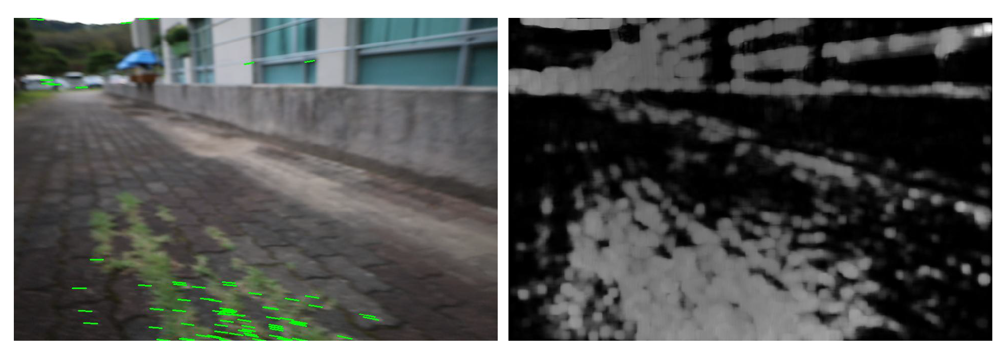
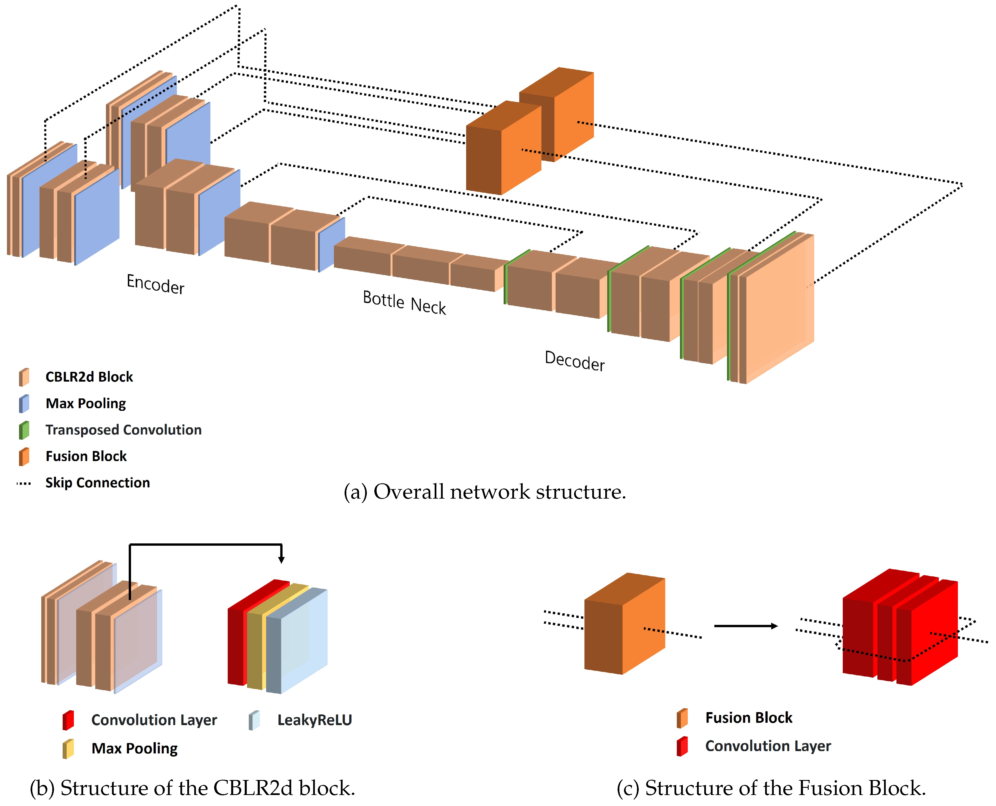
Figure 4.
(Left) Sparse Optical Flow, (Right) Dense Optical Flow.
Figure 5.
Architecture of R-Depth Net. (a) The Defocus Image and Optical Flow are processed by separate encoders, followed by a Fusion Block and a decoder to generate the Depth Map. (b) Structure of the CBLR2d block used in both encoder and decoder, consisting of Convolution, Batch Normalization, and Leaky ReLU. (c) Structure of the Fusion Block that resizes and concatenates the outputs of both encoders before passing to the decoder.
The Gunnar Farneback algorithm outputs both magnitude and direction of motion. While the directional information can be used to estimate the movement direction of the robot, it is less critical for depth estimation. Moreover, incorporating directional data increases the size of the neural network input, thereby raising computational costs. Therefore, in this work, only the magnitude information was utilized.
3. Depth Estimation Network
3.1. R-Depth Net
R-Depth Net takes the defocus image and optical flow image as inputs and produces a depth map representing distance information. As shown in Figure 5a, the network is composed of an encoder, decoder, bottleneck, and fusion block. Skip connections are employed to mitigate information loss between encoder and decoder. Because R-Depth Net incorporates two encoders, the features extracted from both encoders are integrated and dimensionally aligned through the fusion block before being passed to the decoder.
- (1)
- CBLR2d Module
CBLR2d serves as the fundamental building block of R-Depth Net, sequentially performing convolution, batch normalization, and LeakyReLU operations. Figure 5b illustrates the structure of the CBLR2d module.
- (2)
- Fusion Block
To transfer the data extracted from the encoders to the decoder, the outputs of the two encoders must be fused and reshaped into a single representation. In the proposed model, this process is performed by the fusion block, as illustrated in Figure 5c, which integrates the features and adjusts their dimensions before passing them to the decoder.
3.2. Training
R-Depth Net is trained in a supervised learning manner, where the network is optimized to minimize the loss between the predicted depth maps and the ground truth. The Adam (Adaptive Moment Estimation) optimizer was employed for the optimization process.
3.3. Loss Function
The objective of R-Depth Net is to estimate depth maps, and for this purpose, BerHu loss and gradient loss were employed [17,18]. BerHu combines the robustness of L1 with the smoothness of L2. While L1 loss is robust to outliers, it contains non-differentiable points due to its structure. On the other hand, L2 loss is differentiable everywhere but is highly sensitive to outliers. BerHu loss was designed to compensate for the drawbacks of both L1 and L2 losses. Equation (4) represents the L1 loss, Equation (5) represents the L2 loss, and Equation (6) defines the BerHu loss.
Gradient loss is a loss function that computes the difference between the per-pixel gradients of the predicted depth map and those of the ground truth data. To calculate the gradients, the filters defined in Equation (7) were applied, and the differences between gradients were measured using the L1 loss.
To compute the final loss from the BerHu loss and the gradient loss, weighted summation was applied to each component. The final loss, , is defined as in Equation (8), where and .
3.4. Training Result
The training results are visually presented in Figure 6 and were quantitatively evaluated using a test dataset that was not included in the training process. The quantitative outcomes are summarized in Table 2 and Table 3.
Table 2 reports the results based on the accuracy under threshold metric, which measures the percentage of predictions that fall within a multiplicative factor of the ground truth. The proposed model achieved an accuracy of 95
Table 3 evaluates the depth estimation error using three metrics. The absolute relative error (AbsRel) was 0.065, the squared relative error (SqRel) was 0.062, and the root mean square error (RMSE) was 0.55 m. These results demonstrate the effectiveness and potential of R-Depth Net for accurate depth estimation.
4. Obstacle Detection and Height Estimation
4.1. Obstacle Detection
For obstacle detection, a preprocessing step is required to separate the ground from other objects in the input image. In this work, a separation method based on depth variation patterns was adopted. When the camera observes the ground at a fixed angle, the ground depth tends to gradually increase along the vertical direction. In contrast, obstacles exhibit nearly constant depth values at specific positions, showing minimal variation. Leveraging these distance variation characteristics, we designed an obstacle detection algorithm that separates ground and obstacles based on pixel-level depth gradients.
Figure 10 presents an image of obstacle depth. In Figure 10(a), the depth profile along the red line is shown in Figure 10(b). In Figure 10(b), Box 1 corresponds to the obstacle depth values, while Box 2 corresponds to the ground depth values. It can be observed that the ground region exhibits a steeper gradient than the obstacle region.
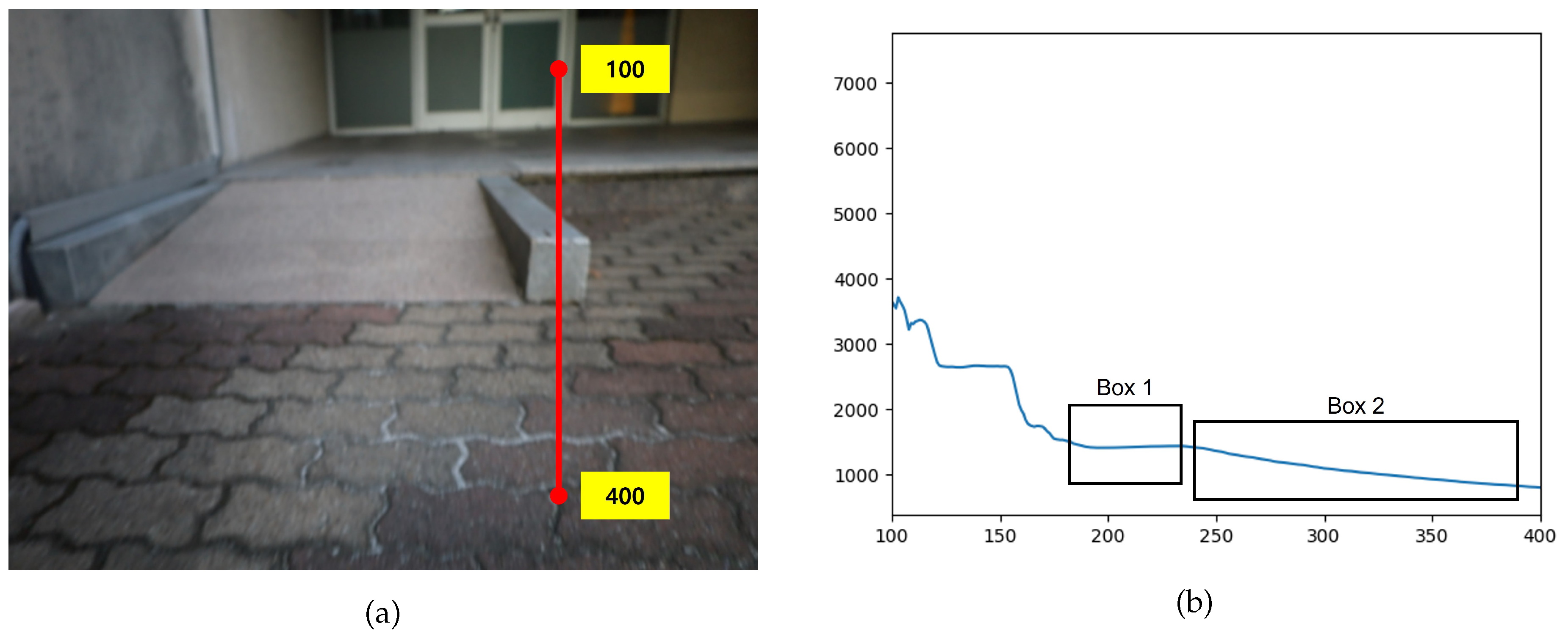
Figure 7.
Depth variation profile for obstacle detection. (a) Sample Column Representing Depth. (b) Depth Profile with Box 1 Representing the Obstacle and Box 2 Representing the Ground (Horizontal Axis: Pixel Coordinates, Vertical Axis: Depth).
Figure 7.
Depth variation profile for obstacle detection. (a) Sample Column Representing Depth. (b) Depth Profile with Box 1 Representing the Obstacle and Box 2 Representing the Ground (Horizontal Axis: Pixel Coordinates, Vertical Axis: Depth).
To analyze these depth variation characteristics, this study generated a V-disparity map [19]. A disparity map is constructed by accumulating the frequency of identical depth values along each horizontal scanline of the image. In the resulting two-dimensional histogram, the vertical axis represents depth values, while the horizontal axis represents the frequency of occurrence of each depth. Figure 8 provides an example. In the first row of Figure 8, a depth value of 3 m appears three times; consequently, the V-disparity map records the value 3 at the position corresponding to a depth of 3 m. In this work, the range of V-disparity map values was normalized to fall between 0 and 500 for depths within 3 m, allowing for a more detailed representation.
Using the ground candidate regions extracted from the V-disparity map, a ground mask was generated. Regions that do not overlap with this mask were classified as obstacles, while the overlapping boundaries were regarded as the lower edges of the obstacles. The resulting mask is shown in Figure 9.
For the upper boundary of obstacles, the regions located above the lower points of the obstacles in the same column of the V-disparity map were identified as obstacle areas. Figure 10 illustrates obstacle region detection using the V-disparity map, where the red boxed areas indicate the detected obstacle regions.
4.2. Height Estimation
The obstacle height must be estimated using the lower and upper boundary information obtained from the obstacle detection algorithm. The actual height is derived as illustrated in Figure 11. The ratio between the real height of the obstacle and the number of pixels in the image corresponds to the distance between the obstacle and the camera, as well as the focal length of the camera. By rearranging this relationship, the actual obstacle height can be expressed as Equation(9).
5. Experiment
The height estimation experiments in this work were conducted using a quadruped robot platform. Specifically, the Go1 platform developed by Unitree Robotics was employed, which supports a step-over mode for obstacle negotiation. As shown in Figure 12, the step-over mode features a higher leg lift, making it advantageous for overcoming relatively large obstacles.
In the experiments, the maximum negotiable obstacle height was set to 18 cm. When the predicted obstacle height was below this threshold, the robot attempted to traverse the obstacle in step-over mode. Conversely, If the predicted height exceeded 18 cm, the robot switched to step-over mode or stopped; otherwise it used normal gait.
All control commands and neural network computations were executed on a processing unit equipped with an Intel Core i5-1135G7 CPU, 16 GB of memory, and an NVIDIA GeForce MX450 GPU. The inference speed achieved was approximately 4 FPS.
5.1. Experiment on the Effects of Depth from Defocus and Optical Flow
This experiment was conducted to assess the impact of defocus images and optical flow information on depth estimation accuracy. The evaluation was carried out under three conditions: (1) using both defocus image data and optical flow data simultaneously, (2) using only defocus image data, and (3) using image data without defocus applied. The evaluation results are summarized in Table 4.
When defocus images were incorporated, the absolute relative error (AbsRel) was significantly reduced from 0.68 to 0.29. Furthermore, the inclusion of optical flow information led to an additional improvement, reducing the error from 0.29 to 0.24.
5.2. Experiment on Obstacle Distance Estimation Accuracy
To evaluate the accuracy of R-Depth Net in predicting the depth between obstacles and the vision camera, measurements were conducted at intervals of 0.5 m from 1 m to 3 m. Figure 13 shows a scene from the experiment, and the results are summarized in Table 5.
In the experiment measuring obstacle distance estimation accuracy, R-Depth Net demonstrated errors of 0.3 m in terms of RMSE and 0.26 m in terms of MAE.
5.3. Experiment on Obstacle Height Estimation Accuracy
An experiment was conducted to evaluate the accuracy of obstacle height estimation using R-Depth Net in conjunction with the obstacle height estimation algorithm. As shown in Figure 14, the experimental setup included step-height obstacles of three different heights: 0.1 m, 0.15 m, and 0.2 m. The results are summarized in Table 6.
The results of obstacle height estimation revealed errors of 4.8 cm in terms of RMSE and 4 cm in terms of MAE. It was observed that the estimation error increased as the obstacle height increased.
5.4. Experiment on Obstacle Overcoming in Real-World Environments
To evaluate the practical applicability of the proposed R-Depth Net and obstacle height estimation algorithm, experiments were conducted on obstacles of varying heights. Figure 15 illustrates the process of detecting obstacles and estimating their heights, Figure 16 shows the robot overcoming an obstacle, and Figure 17 presents a case where the robot stopped upon determining that the obstacle could not be negotiated.
In most cases, the obstacle heights were accurately predicted, and appropriate control actions were executed accordingly. However, some prediction errors were observed. In Case 2 of Figure 15, although the obstacle was detected, errors in distance estimation resulted in its height being underestimated. This was attributed to calibration errors in the distance-based correction during the depth estimation process. In Case 5, the obstacle was too tall, causing the V-disparity–based detection to fail, and as a result, the obstacle was not recognized at all.
5.5. Experiment Result
Experiments were conducted to evaluate the effects of depth from defocus and optical flow, the accuracy of obstacle distance estimation, the accuracy of obstacle height estimation, and the robot’s performance in overcoming obstacles in real environments. In the experiment on the effects of defocus and optical flow, the absolute relative error (AbsRel) decreased from 0.68 to 0.29 when depth from defocus was applied, and further decreased from 0.29 to 0.24 with the addition of optical flow.
The obstacle distance estimation experiment was performed by measuring target distances at 0.5 m intervals within the range of 1 m to 3 m. The results showed that the proposed neural network–based model achieved an error of 0.3 m in terms of RMSE and 0.26 m in terms of MAE. In the obstacle height estimation experiment, overall errors of 0.048 m in terms of RMSE and 0.04 m in terms of MAE were observed.
Finally, obstacle negotiation experiments were conducted in real environments. Depending on the estimated obstacle height, the robot appropriately switched to obstacle-overcoming mode or issued a stop command. Since real-world obstacle negotiation relies on comprehensive analysis of multiple V-disparity maps and references to height values from previous frames, defocus image, the system maintained accurate height estimation and reliable mode switching despite the presence of errors in depth estimation.
Through these experiments, it was demonstrated that the proposed monocular depth estimation method is well suited for robotic applications and is effective for obstacle detection using monocular vision.
6. Conclusion
We presented R-Depth Net, a monocular metric depth estimator that fuses depth-from-defocus and optical-flow cues, and an obstacle height estimation pipeline for traversal decisions on a quadruped. The R-Depth Net, designed for depth estimation, takes defocus images and optical flow information as inputs, and experimental results confirmed that these cues significantly enhance depth estimation performance.
When defocus information was applied, the absolute relative error (AbsRel) decreased from 0.68 to 0.29, and the inclusion of optical flow further reduced the error to 0.24. In obstacle distance estimation experiments, the proposed model achieved an RMSE of 0.30 m and an MAE of 0.26 m, while in obstacle height estimation experiments, it recorded an RMSE of 0.048 m and an MAE of 0.040 m. The proposed depth estimation and height prediction algorithm was successfully implemented on a quadruped robot platform, where the robot autonomously switched walking modes or stopped based on obstacle height. By leveraging multi-frame V-disparity analysis and cumulative prediction, the system maintained stable performance despite occasional depth estimation errors.
The results demonstrates that real-time obstacle detection and traversal decision-making can be achieved solely through monocular vision–based depth estimation, without the need for complex sensors or expensive equipment.
Author Contributions
Conceptualization, S.A. and D.C.; methodology, S.A.; software, S.A. and Y.K.; validation, S.A. and D.C.; formal analysis, D.C.; investigation, D.C.; resources, S.A.; data curation, S.C. and S.A; writing—original draft preparation, S.A.; writing—review and editing, D.C.; visualization, S.C. and Y.K.; supervision, D.C.; project administration, D.C.; funding acquisition, D.C. All authors have read and agreed to the published version of the manuscript.
Funding
This work was supported by the National Research Foundation of Korea(NRF) grant funded by the Korea government(MSIT) (RS-2025-23525689).
Institutional Review Board Statement
Not applicable.
Informed Consent Statement
Not applicable.
Conflicts of Interest
The authors declare no conflict of interest.
Abbreviations
The following abbreviations are used in this manuscript:
| LiDAR | Light Detection and Ranging |
| DfD | Depth from Defocus |
| OF | Optical Flow |
| CBLR2d | Convolution–Batch Normalization–Leaky ReLU (2D) |
| RMSE | Root Mean Squared Error |
| MAE | Mean Absolute Error |
| AbsRel | Absolute Relative Error |
| SqRel | Squared Relative Error |
| FPS | Frames Per Second |
| CPU | Central Processing Unit |
| GPU | Graphics Processing Unit |
| Adam | Adaptive Moment Estimation |
References
- A. Carballo et al., "LIBRE: The Multiple 3D LiDAR Dataset," 2020 IEEE Intelligent Vehicles Symposium (IV), Las Vegas, NV, USA, 2020, pp. 1094–1101. [CrossRef]
- W. Boonsuk, "Investigating effects of stereo baseline distance on accuracy of 3D projection for industrial robotic applications," 5th IAJC/ISAM Joint International Conference, 2016, pp. 94–98.
- Z. Cai and C. Metzler, "Underwater Monocular Metric Depth Estimation: Real-World Benchmarks and Synthetic Fine-Tuning," arXiv preprint arXiv:2507.02148, 2025. [CrossRef]
- X. Dong, M. A. Garratt, S. G. Anavatti and H. A. Abbass, "Towards Real-Time Monocular Depth Estimation for Robotics: A Survey," IEEE Trans. Intell. Transp. Syst., vol. 23, no. 10, pp. 16940–16961, Oct. 2022. [CrossRef]
- A. Gurram, A. F. Tuna, F. Shen, O. Urfalioglu and A. M. López, "Monocular Depth Estimation Through Virtual-World Supervision and Real-World SfM Self-Supervision," IEEE Trans. Intell. Transp. Syst., vol. 23, no. 8, pp. 12738–12751, Aug. 2022. [CrossRef]
- J. Zhang, "Survey on Monocular Metric Depth Estimation," arXiv preprint arXiv:2501.11841, 2025. [CrossRef]
- R. Xiaogang, Y. Wenjing, H. Jing, G. Peiyuan and G. Wei, "Monocular Depth Estimation Based on Deep Learning: A Survey," 2020 Chinese Automation Congress (CAC), Shanghai, China, 2020, pp. 2436–2440. [CrossRef]
- A. Bochkovskii et al., "Depth Pro: Sharp monocular metric depth in less than a second," arXiv preprint arXiv:2410.02073, 2024. [CrossRef]
- S. F. Bhat et al., "ZoeDepth: Zero-shot transfer by combining relative and metric depth," arXiv preprint arXiv:2302.12288, 2023. [CrossRef]
- T. Shiozaki and G. Dissanayake, "Eliminating scale drift in monocular SLAM using depth from defocus," IEEE Robot. Autom. Lett., vol. 3, no. 1, pp. 581–587, Jan. 2018. [CrossRef]
- T. Shimada et al., "Fast and high-quality monocular depth estimation with optical flow for autonomous drones," Drones, vol. 7, no. 2, p. 134, 2023. [CrossRef]
- M. Carvalho et al., "Deep depth from defocus: how can defocus blur improve 3D estimation using dense neural networks?," in Proc. ECCV Workshops, 2018, pp. 1–17.
- N. Silberman, D. Hoiem, P. Kohli and R. Fergus, "Indoor segmentation and support inference from RGBD images," in Computer Vision – ECCV 2012, LNCS, vol. 7576, Springer, Berlin, Heidelberg, pp. 746–760, 2012. [CrossRef]
- M. Subbarao and G. Surya, "Depth from defocus: A spatial domain approach," Int. J. Comput. Vis., vol. 13, no. 3, pp. 271–294, 1994. [CrossRef]
- S. M. Ahn and D. Choi, "Development of image registration algorithms for collecting depth from defocus datasets," Trans. Korean Soc. Mech. Eng. A, vol. 49, no. 1, pp. 11–16, 2025. [CrossRef]
- G. Farnebäck, "Two-frame motion estimation based on polynomial expansion," in Image Analysis, SCIA 2003, LNCS, vol. 2749, Springer, Berlin, Heidelberg, pp. 363–370, 2003. [CrossRef]
- L. Zwald and S. Lambert-Lacroix, "The BerHu penalty and the grouped effect," J. Nonparametric Stat., vol. 28, no. 3, pp. 487–514, 2016. [CrossRef]
- J. Hu, M. Ozay, Y. Zhang and T. Okatani, "Revisiting Single Image Depth Estimation: Toward Higher Resolution Maps With Accurate Object Boundaries," 2019 IEEE Winter Conf. Appl. Comput. Vis. (WACV), Waikoloa, HI, USA, 2019, pp. 1043–1051. [CrossRef]
- H.-C. Huang et al., "An Indoor Obstacle Detection System Using Depth Information and Region Growth," Sensors, vol. 15, no. 10, pp. 27116–27141, 2015. [CrossRef]
Figure 1.
Data collection hardware.
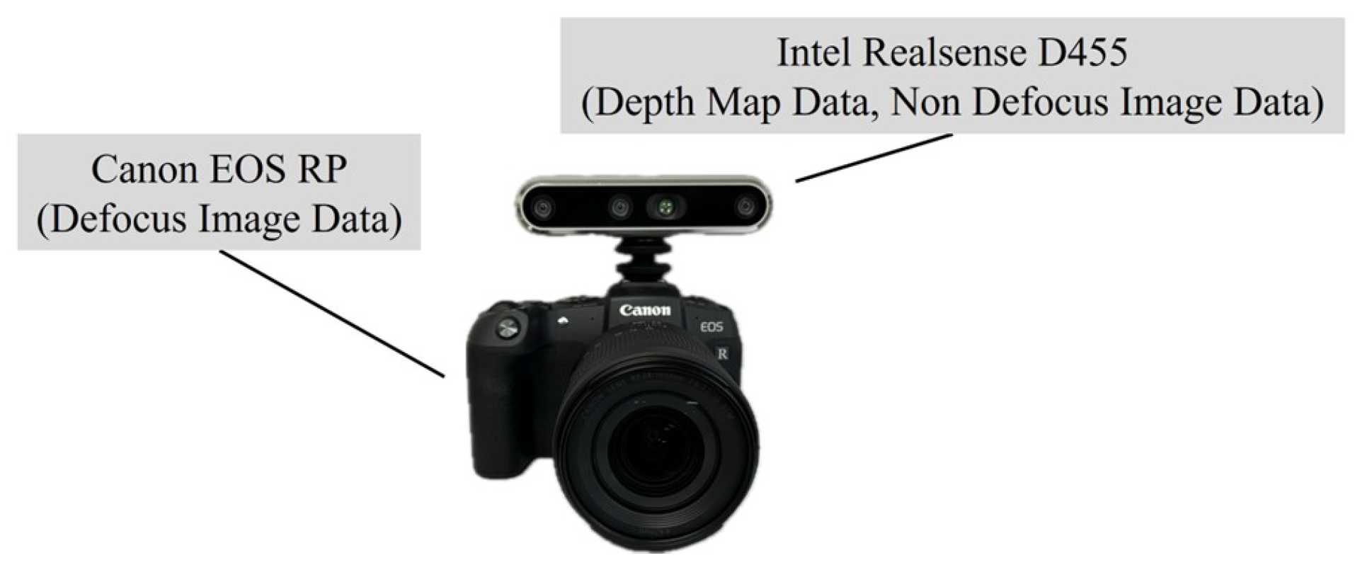
Figure 2.
Compare the degree of blur based on distance (from left to right, 180 cm, 120 cm, 60 cm).
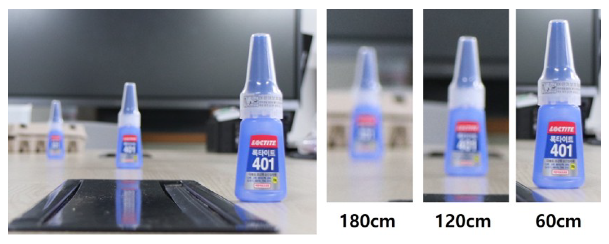
Figure 3.
Cross-section of a thin lens.
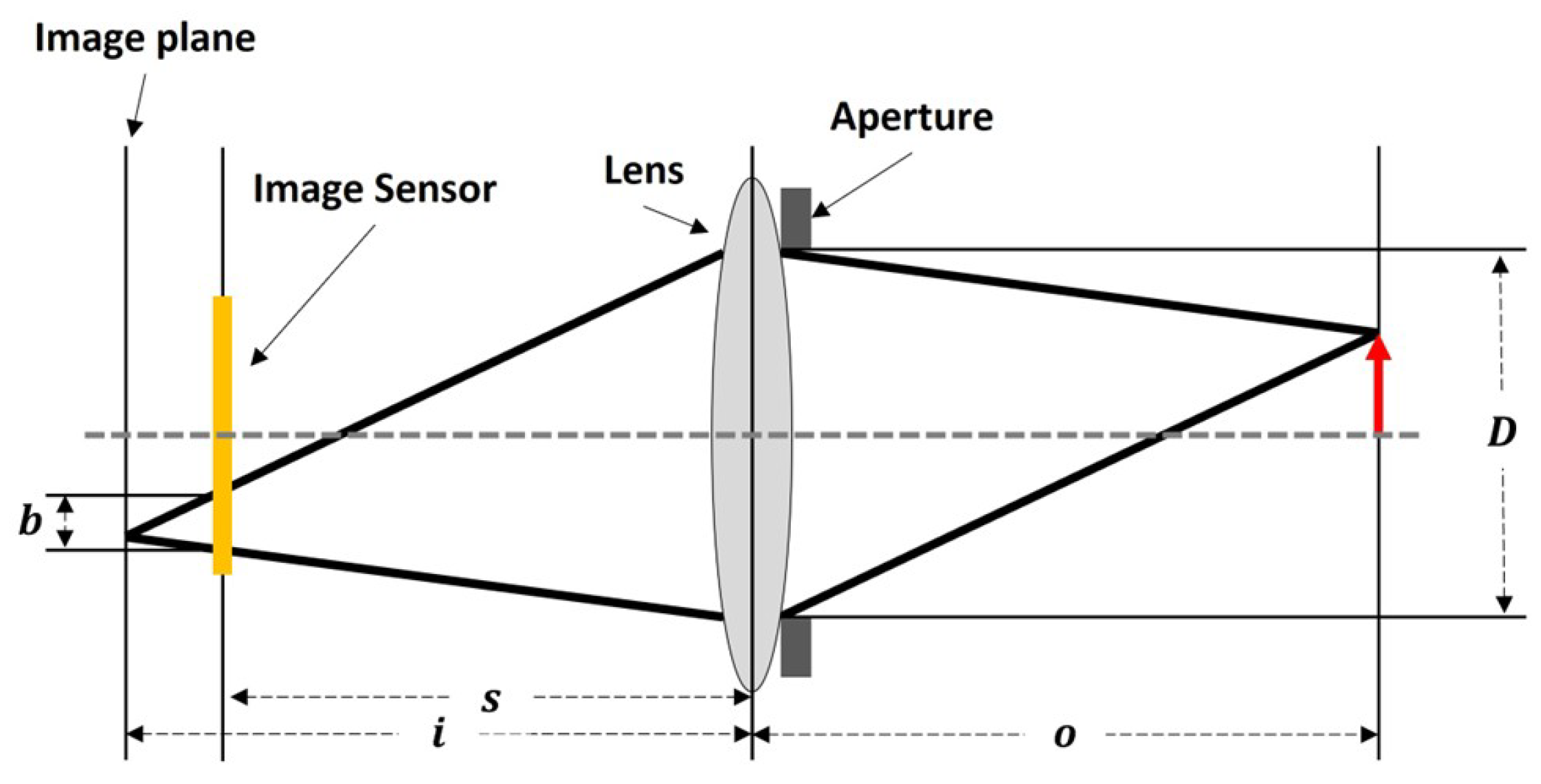
Figure 6.
Training Result
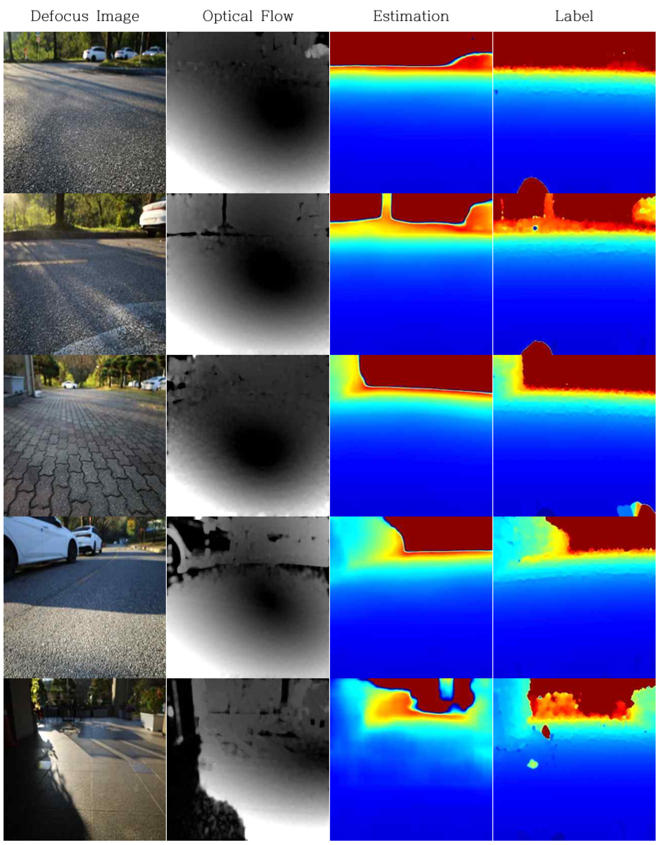
Figure 8.
Example of a V-Disparity Map.
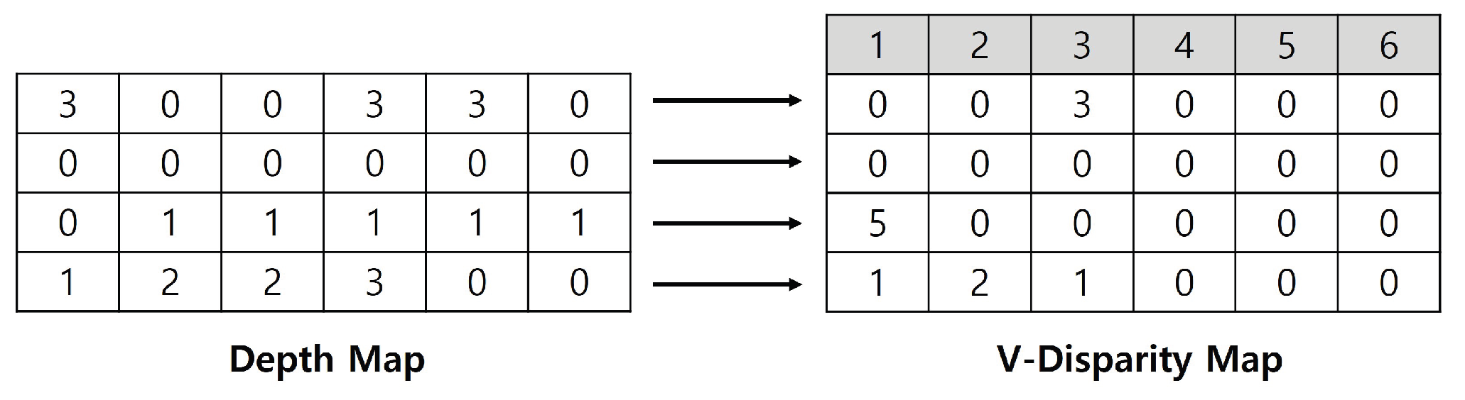
Figure 9.
Example of Ground Mask.

Figure 10.
Detection of obstacle regions using the V-Disparity map.
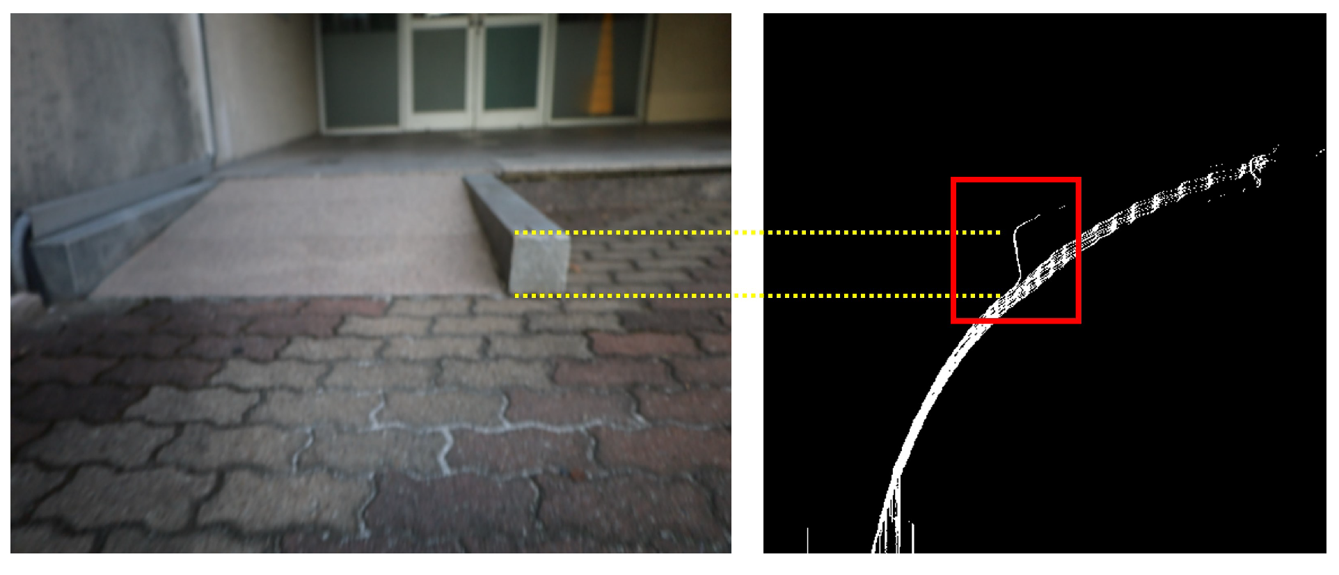
Figure 11.
Relationship Between Camera and Obstacles for Height Calculation.
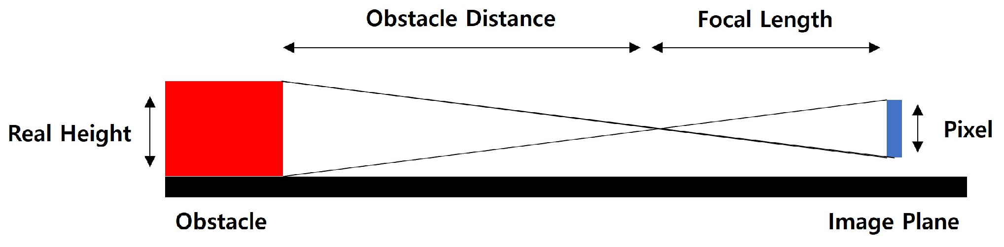
Figure 12.
Unitree Go1 Walking Mode (Left : Normal Walking Mode, Right : Obstacle Overcoming Mode).
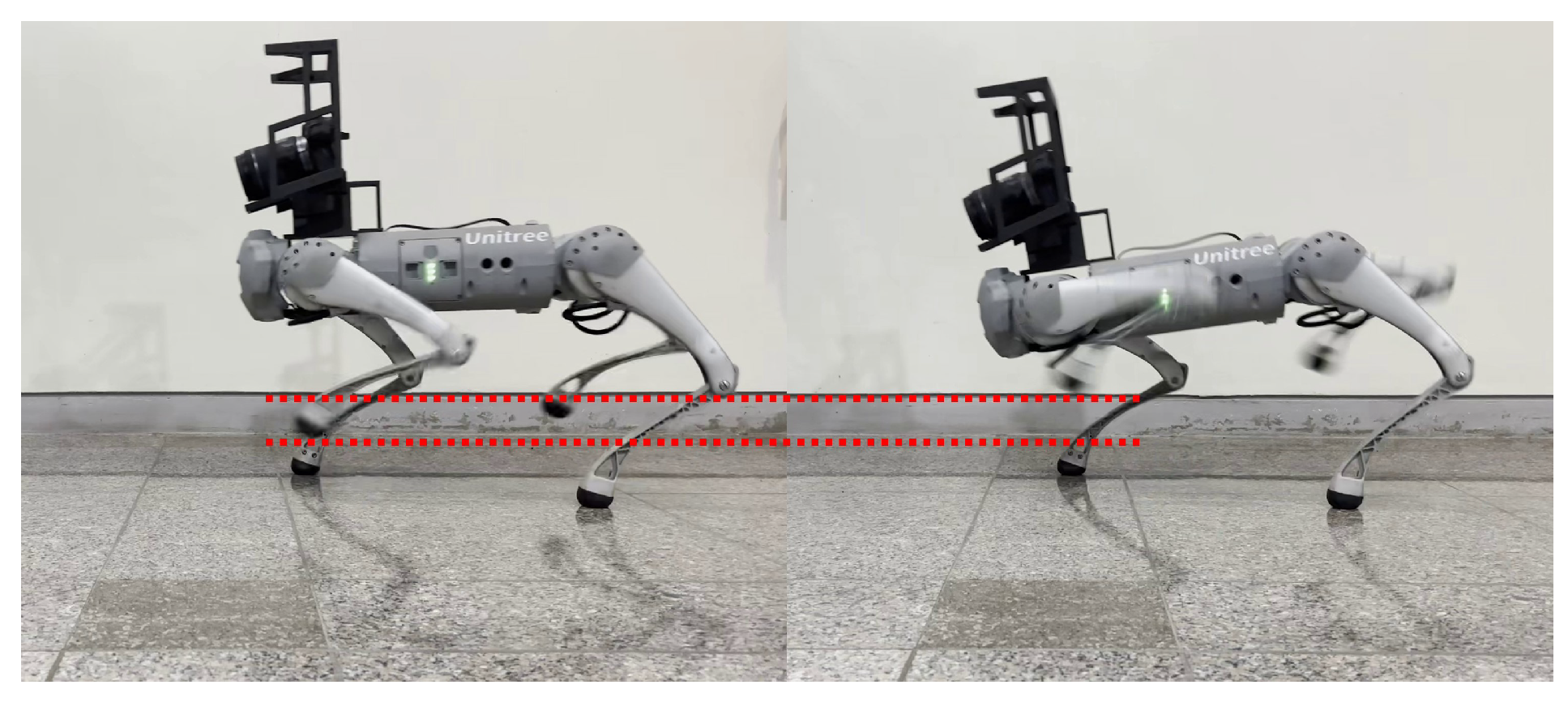
Figure 13.
Experimental Environment for Obstacle Distance Estimation Accuracy.
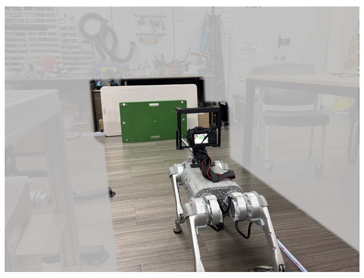
Figure 14.
Experimental Environment for Obstacle Height Estimation Accuracy.
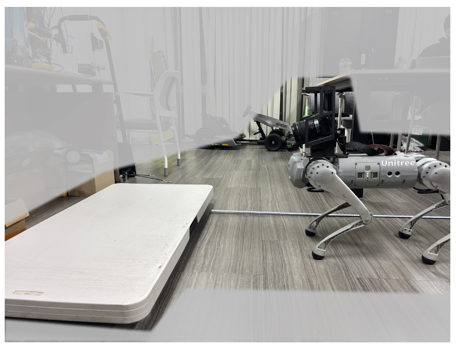
Figure 15.
Obstacle Height Estimation in Real-World Environments (Green dot:obstacle top, Blue dot:obstacle bottom).
Figure 15.
Obstacle Height Estimation in Real-World Environments (Green dot:obstacle top, Blue dot:obstacle bottom).
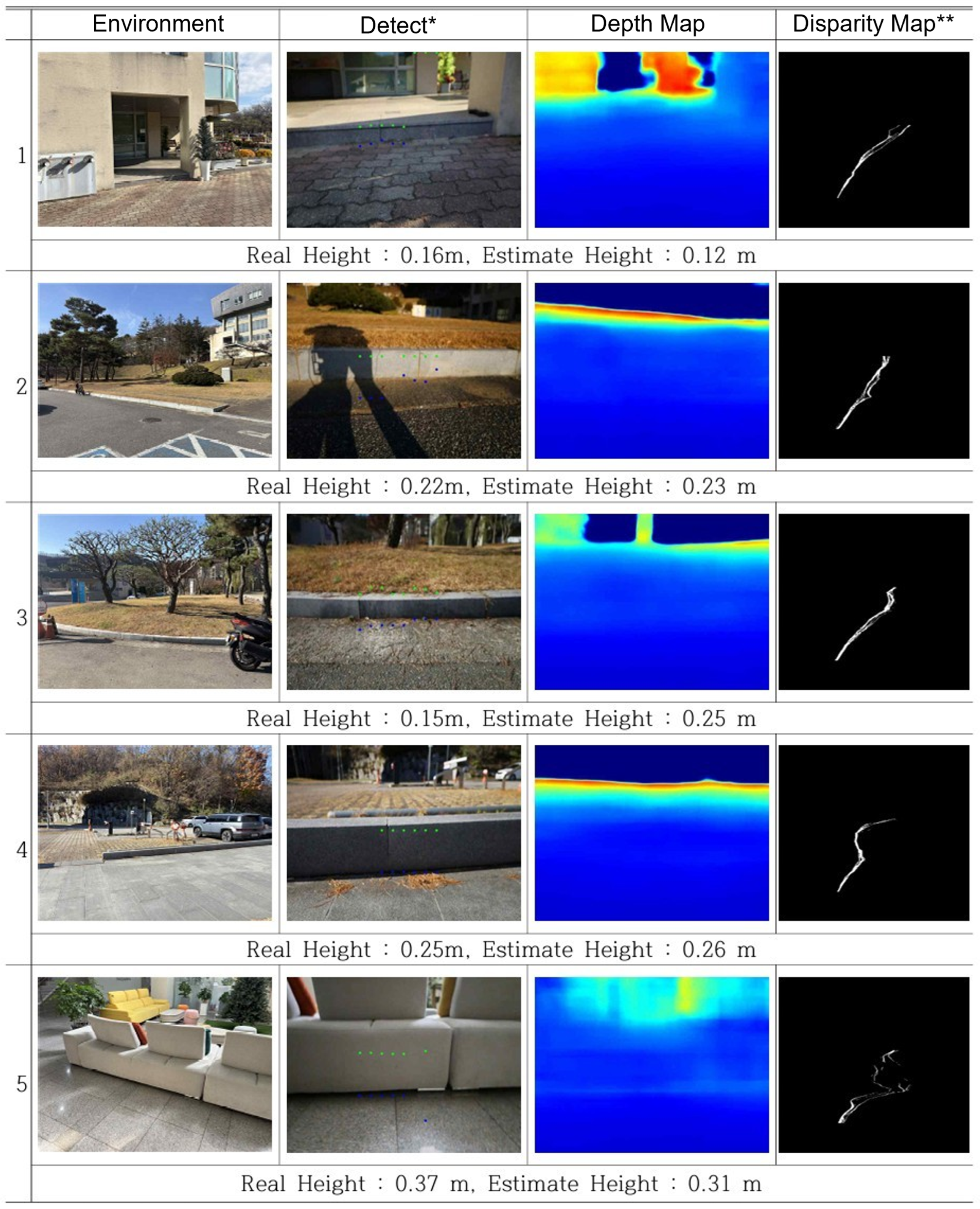
Figure 16.
Obstacle Detection and Overcome Mode Transition in Real-World Environments (1st row:Experimental Environment, 2nd row:Robot View, 3rd row:Optical Flow, 4th row:Predicted Depth Map, 5th row:V-Disparity Map).
Figure 16.
Obstacle Detection and Overcome Mode Transition in Real-World Environments (1st row:Experimental Environment, 2nd row:Robot View, 3rd row:Optical Flow, 4th row:Predicted Depth Map, 5th row:V-Disparity Map).
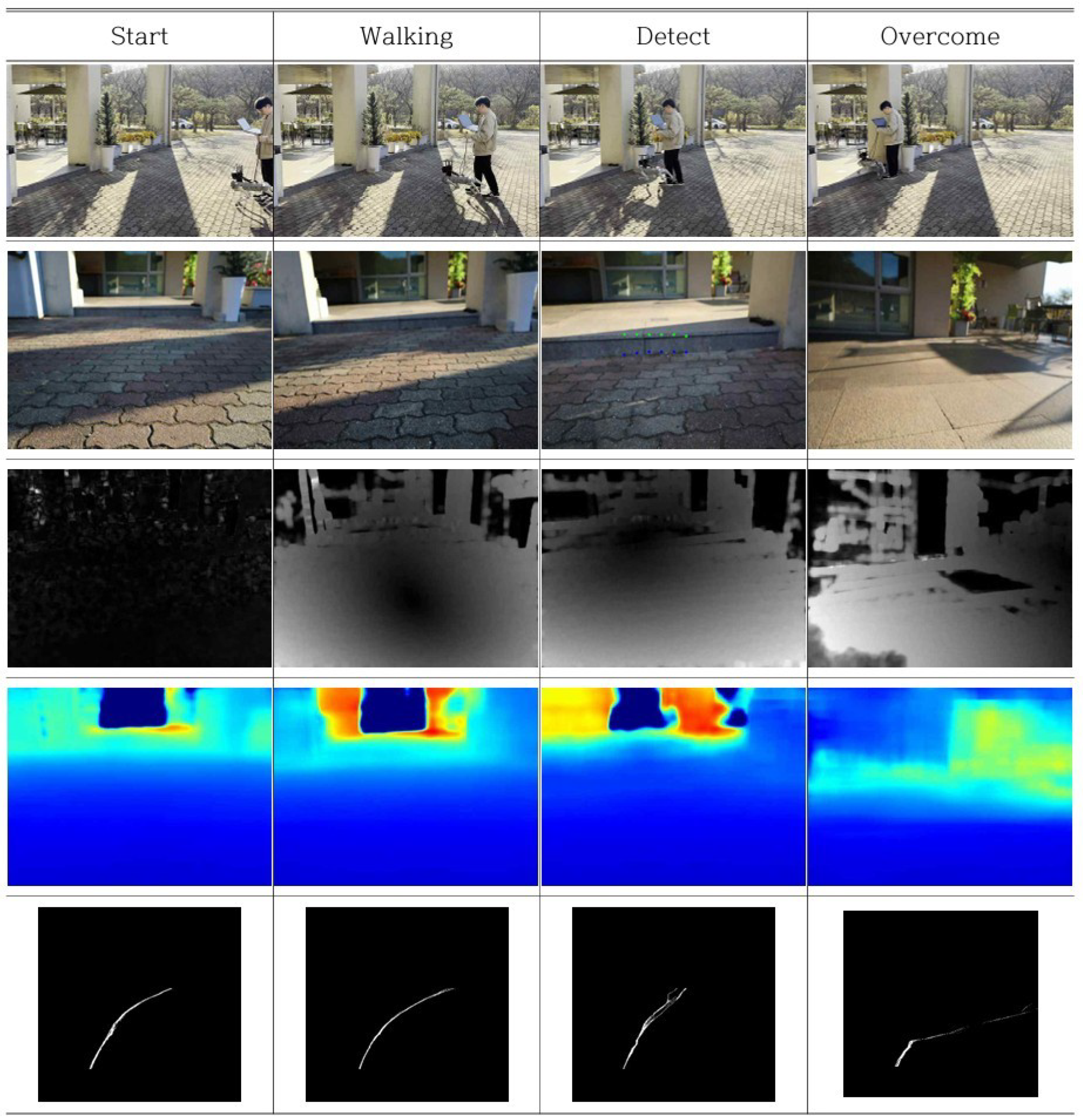
Figure 17.
Obstacle Detection and Stop Mode Transition in Real-World Environments (1st row:Experimental Environment, 2nd row:Robot View, 3rd row:Optical Flow, 4th row:Predicted Depth Map, 5th row:V-Disparity Map).
Figure 17.
Obstacle Detection and Stop Mode Transition in Real-World Environments (1st row:Experimental Environment, 2nd row:Robot View, 3rd row:Optical Flow, 4th row:Predicted Depth Map, 5th row:V-Disparity Map).
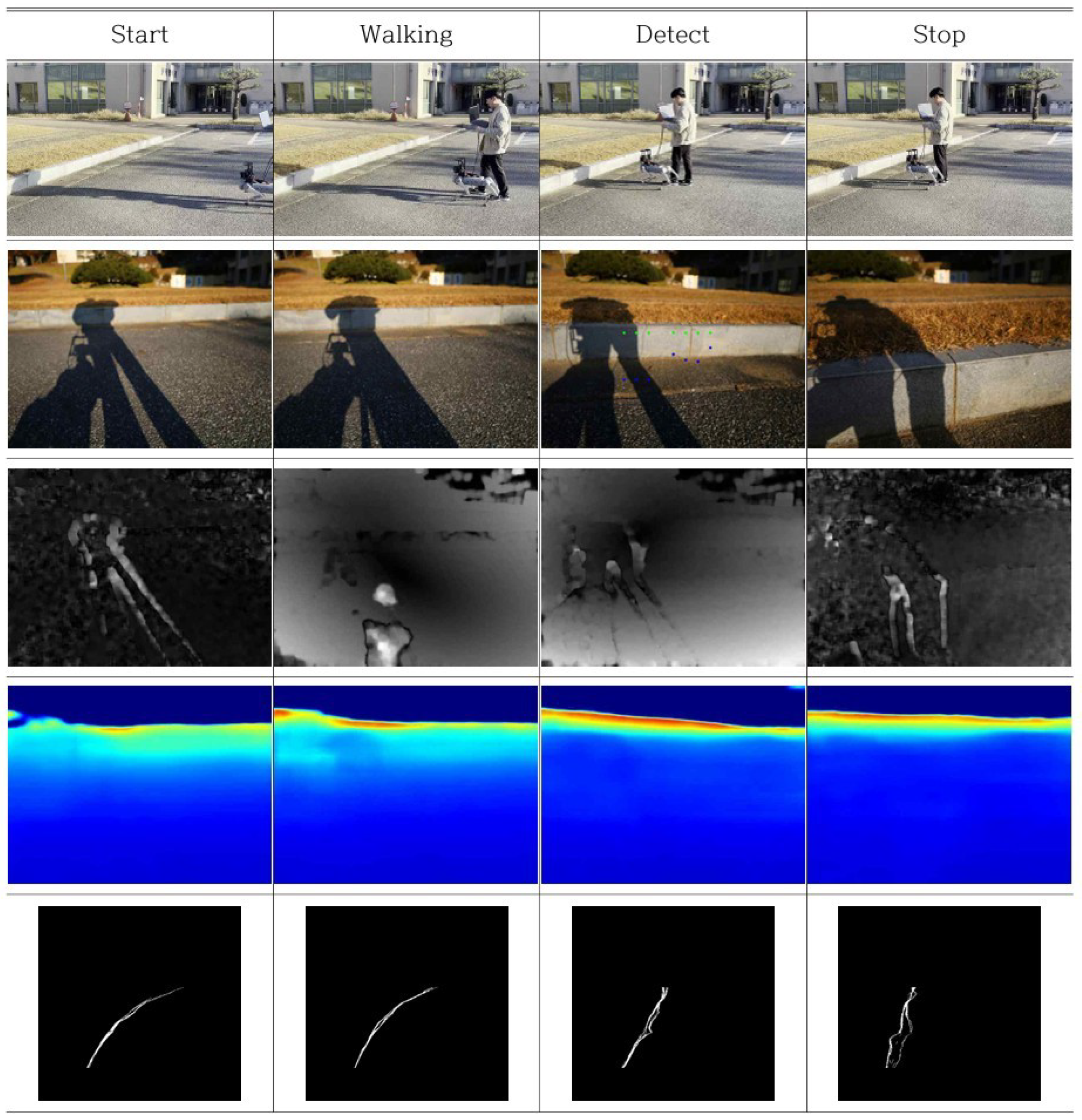

Table 1.
Variables Used to Calculate the degree of blur.
| Symbol | Meaning |
|---|---|
| s | Distance between lens and image sensor |
| f | Focal length |
| i | Distance between lens and image plane |
| b | Amount of blur |
| o | Distance between lens and object |
| D | Aperture diameter |
Table 2.
Training Result – Accuracy.
| Metric | Value |
|---|---|
| 95% | |
| 97% | |
| 98% |
Table 3.
Training Result – Error.
| Metric | Value |
|---|---|
| Absolute Relative Error (AbsRel) | 0.065 |
| Squared Relative Error (SqRel) | 0.062 |
| Root Mean Squared Error (RMSE) | 0.55 m |
Table 4.
Impact of Depth from Defocus and Optical Flow on Test Dataset.
| Method | AbsRel | SqRel |
|---|---|---|
| No Defocus | 0.68 | 0.13 |
| Defocus | 0.29 | 0.05 |
| Defocus + Optical Flow | 0.24 | 0.04 |
Table 5.
Distance Estimation Error of R-Depth Net.
| Distance | RMSE (m) | MAE (m) |
|---|---|---|
| 3 m | 0.45 | 0.45 |
| 2.5 m | 0.06 | 0.05 |
| 2 m | 0.20 | 0.20 |
| 1.5 m | 0.29 | 0.29 |
| 1 m | 0.32 | 0.32 |
| Average | 0.30 | 0.26 |
Table 6.
Obstacle Estimation Error.
| Obstacle Height | RMSE [m] | MAE [m] |
|---|---|---|
| 0.1 m | 0.03 | 0.029 |
| 0.15 m | 0.039 | 0.035 |
| 0.2 m | 0.064 | 0.054 |
| Total | 0.048 | 0.04 |
Disclaimer/Publisher’s Note: The statements, opinions and data contained in all publications are solely those of the individual author(s) and contributor(s) and not of MDPI and/or the editor(s). MDPI and/or the editor(s) disclaim responsibility for any injury to people or property resulting from any ideas, methods, instructions or products referred to in the content. |
© 2025 by the authors. Licensee MDPI, Basel, Switzerland. This article is an open access article distributed under the terms and conditions of the Creative Commons Attribution (CC BY) license (http://creativecommons.org/licenses/by/4.0/).
Copyright: This open access article is published under a Creative Commons CC BY 4.0 license, which permit the free download, distribution, and reuse, provided that the author and preprint are cited in any reuse.


