Submitted:
24 September 2025
Posted:
25 September 2025
You are already at the latest version
Abstract
The Kawahara equation and its modified form are nonlinear dispersive partial differential equations commonly used to model wave propagation in fluids and plasmas. In hemodynamic studies, these equations have been adapted to describe the propagation of pulse waves in large arteries, where dispersive wave effects play an important role in capturing the dynamics of blood flow. In this study, we focus on their time fractional generalizations within the Caputo sense and construct approximate analytical solutions by employing the optimal auxiliary function method (OAFM). This technique generates auxiliary functions with adjustable parameters, which enhances both accuracy and convergence speed. By applying OAFM to the time fractional Caputo Kawahara (TCFKE) and modified Kawahara (MTCFKE) equations, we obtain symmetric approximate solutions and confirm their efficiency through numerical tests and graphical illustrations. Moreover, in the context of fluid flow and shallow water wave propagation, comparative analysis with other existing methods including the homotopy analysis method, residual power series method, and natural transform decomposition technique highlights the robustness and higher accuracy of OAFM.
Keywords:
Kawahara equation
; Caputo operator
; optimal auxiliary function
1. Introduction
The governing equations of wave motion play a crucial role in physics, fluid dynamics, and applied mathematics. Among these, the Kawahara equation, first introduced by Kawahara in 1970 [1], describes solitary wave propagation in different media [2,3]. This equation has been further generalized to explore conservation laws and symmetry properties, particularly in shallow water dynamics and magneto-acoustic wave theory [4]. Applications of the modified Kawahara equation have also been reported in plasma wave studies and capillary-gravity wave problems [5,6,7]. In recent decades, the use of fractional calculus has gained momentum as an effective tool for capturing memory effects and hereditary properties in diverse materials and processes. Fractional partial differential equations provide accurate models across multiple fields, including fluid mechanics, engineering, polymer science, physics, biomedical science, groundwater hydrology, and electrical networks [8,9,10,11]. Partial differential equations (PDEs) also underpin various mathematical concepts, such as the Calabi and Poincaré coefficients, and numerous approximate solution techniques have been developed to study nonlinear PDEs. Researchers have applied different analytical and semi-analytical methods to investigate fractional models of physical and biological systems. Examples include: the homotopy analysis method [12]; and reproducing kernel Hilbert space methods for telegraph, Fornberg-Whitham, and non-local fractional equations [13,14,15]; monotone iterative methods for reaction-diffusion models [16]; direct algebraic mapping techniques for damped KdV equations [17]; the Adams-Bashforth method for Atangana-Baleanu Caputo equations [18]; the modified expansion function approach for nonlinear Schrödinger equations [19]; homotopy perturbation methods [20]; the expansion method for higher-order nonlinear Boussinesq equations [21]; variational iteration methods for nonlinear FPDEs [22]; the sine-Gordon expansion applied to Wu-Zhang systems [23]; the Laplace residual power series method [24]; fractional Newton methods for convergence analysis [25]; the Laplace transform for fuzzy PDEs [26]. Among these, the OAFM has emerged as a versatile tool for tackling nonlinear engineering and physical problems. Originally introduced by Hernández and Beléndez [27] for nonlinear Schrödinger equations, OAFM has since been extended to a variety of applications. For instance, Iqbal et al. [28] applied it to Caputo fractional nonlinear long-wave systems, while Alsheekh et al. [29] employed it for fractional Whitham-Broer-Kaup systems. Other contributions include extending OAFM to fractional PDEs using the complex transform approach [30], modeling synchronous generators [31], and solving generalized PDEs [32,33,34]. Furthermore, OAFM has been applied in epidemiological modeling, such as the nonlinear SEIR system for COVID-19 dynamics [35]. For the TCFKE and its modified form MTCFKE, many methods have been explored, numerical schemes such as the septic B-spline collocation method [36], generalized formulations using analytical techniques [37], the homotopy analysis transform [38], residual power series method (RPSM) [39], the natural transform decomposition method (NTDM) [40], iterative Laplace transforms [41], Laplace-Adomian decomposition [42], Other contributions investigate Kawahara and modified Kawahara equations with variable coefficients using Lie group analysis [43] and the homotopy analysis method (HAM) [44]. As we know that fractional extensions of the Kawahara and modified Kawahara equations capture memory effects in nonlinear wave phenomena more effectively than classical models. However, obtaining accurate solutions for such equations remains challenging, as many existing methods face convergence or accuracy limitations. This work is motivated by the need for a reliable and efficient approach, where the OAFM is applied to derive precise approximate solutions for these fractional models. In this study, we examine the effectiveness of the OAFM for deriving symmetric solutions of the following TCFKE (1) and MTCFKE (2)
and
respectively, where , are constants and is the Caputo operator. Section 2 provides the essential definitions and preliminaries of the Caputo fractional operator. Section 3 outlines the fundamental steps of the OAFM. In Section 4, the OAFM is applied to obtain symmetric solutions of the TCFKE (1) and MTCFKE (2). Section 5 presents numerical simulations and graphical illustrations, where the obtained solutions are compared with those generated by the RPSM [39], the NTDM [40], and the HAM [44]. Finally, Section 6 provides a summary of the main findings along with concluding remarks.
2. On Fractional Derivative
3. Steps of the OAFM
A numerical method or technique for solving a PDE or a system of PDEs is often a collocation method used to obtain approximate solutions. This is done by selecting appropriate collocation points such that the solution lies within a finite-dimensional space of polynomials up to a certain degree, using a finite number of collocation points.
Auxiliary functions are, at the very least, proven to exist, established, or otherwise utilized to achieve the desired outcome.
Here, we present the steps and basic concepts of the OAFM. Consider the general nonlinear Caputo fractional PDE
where and is the nonlinear term consisting .
- Step 1. We take the two components in the first part of (5) to obtain an approximate solution consisting of two components, and , that is,
- Step 3. The first approximate solution depends on the linear equation
- Step 4. The version of expansion of the nonlinear term in (7) is
- Step 7. This method is one of methods that is used to determine the values of and and calculate the square of the residual error
4. Approximate Solutions
As noted earlier, the Kawahara equation and its modified form are nonlinear dispersive partial differential equations primarily used to model wave propagation in fluids and plasmas. In the study of blood flow in arteries, the Kawahara equation has been applied to describe the propagation of pulse waves in large vessels, where dispersive effects play a critical role. By incorporating higher-order dispersion, the equation effectively captures wave deformation and solitary pulse-like structures in arterial hemodynamics. Figure 1 illustrates a fractional-order model of blood flow in arteries [47]. Extending the Kawahara equation to fractional forms further enhances its applicability by accounting for memory and hereditary effects, thereby providing a more realistic mathematical framework for modeling wave propagation in complex biological systems. In this section, we use the OAFM to obtain some approximate solutions of TCFKE (1) and MTCFKE (2).
Example 1.
Consider the following TCFKE
The zero approximations of (14) is given by
Put in (17) to get
Take the auxiliary functions as follows
By the procedure of the OAFM, the first approximation is
Put , and in (21) to get
Take the inverses operator of (22) to obtain
Hence the approximate solution is
Example 2.
Consider the following MTCFKE
where , .
In (25), consider linear term
and nonlinear term is given by
The zero approximations of (25) is given by
Put in (28) to get
Take the auxiliary functions as follows
By the procedure of the OAFM, the first approximation is
Put , and in (32) to get
Take the inverses operator of (33) to obtain
Hence the approximate solution is
5. Numerical Results
This section presents the approximate solutions of the TCFKE (14) and MTCFKE (25) for different fractional orders . The results are summarized in Table 1, Table 2, Table 3 and Table 4, while the corresponding dynamical behaviors are illustrated through numerical simulations in Figure 2, Figure 3, Figure 4, Figure 5, Figure 6, Figure 7 and Figure 8.
Table 1 reports a comparison of the absolute error (AE) between the exact solution of TCFKE (14) at , , and the approximate solutions obtained using three approaches: the present OAFM-based method, the RPSM [39], and the NTDM [40].
In Table 2, approximate solutions of TCFKE (14) are provided for with different fractional orders and values of , computed via OAFM and compared against the RPSM [39] and NTDM [40]. The numerical constants used for the solution in (24) are , , and .
For the MTCFKE, Table 3 highlights comparisons at , , and , with varying values of and . The OAFM results are contrasted with those obtained using RPSM [39] and HAM [44]. Table 4 further examines the MTCFKE for and , again comparing OAFM with RPSM, NTDM [40], and HAM [44]. The constants in the solution of (35) are , , and .
The graphical outcomes supplement these tabulated comparisons. Figure 2 displays the solutions for Example (1) and Example (2) at , , under different values. Figure 3 and Figure 4 extend this analysis to and , respectively. Figure 5 provides surface plots for the TCFKE at with , alongside MTCFKE plots at the same values with , , and . Figure 6 and Figure 7 depict surface plots of both equations at fractional orders and , respectively, while Figure 8 corresponds to .
Overall, the presented tables and figures confirm the accuracy and reliability of OAFM. The tabulated data demonstrate its competitiveness with other established approaches, while the graphical results highlight the symmetry and consistency of the approximate solutions across different fractional orders.
The findings confirm that OAFM produces approximate solutions that closely align with both exact and numerical results, thereby validating its reliability. The method is systematic and straightforward, avoiding the need for linearization, discretization, or perturbation procedures, which simplifies its application. Furthermore, OAFM provides solutions in the form of rapidly convergent series, ensuring both stability and high accuracy.
A notable advantage of OAFM is its wide applicability: it can be employed for both linear and nonlinear fractional differential equations with varying fractional orders. From a computational standpoint, it is more efficient than many conventional numerical approaches, requiring fewer operations to achieve similar levels of accuracy. In addition, the method naturally integrates fractional derivatives and integral operators, making it well-suited for modern fractional models. Finally, the series-based representation of the solutions offers flexibility in accuracy control, as additional terms can be incorporated to enhance the approximation near the exact solution, thereby striking a balance between computational cost and precision.
6. Conclusions
In this study, we applied the OAFM to derive approximate analytical solutions of the TCFKE and its modified form, the MTCFKE. By optimizing auxiliary parameters, the OAFM produced highly accurate and rapidly convergent solutions, which were validated through numerical simulations and graphical analysis. Comparative results with established methods, including the HAM, RPSM, and NTDM, confirmed the reliability, efficiency, and superiority of the OAFM in handling fractional nonlinear wave equations.
The findings highlight the OAFM as a versatile and systematic tool for solving fractional differential models arising in applied sciences, physics, and engineering.
For future work, several promising directions arise from this study. The proposed methodology can be extended to other nonlinear dispersive equations, higher-dimensional systems, and models with variable coefficients. Incorporating different fractional operators—such as the Atangana–Baleanu or Caputo–Fabrizio derivatives—would broaden its applicability and allow for the investigation of nonlocal dynamics with non-singular kernels.
Author Contributions
Formal analysis, Hasan Nihal Zaidi and Amira S. Awaad; Funding acquisition, Ali Tedjani and A.H.A. Alfedeel; Investigation, Hasan Nihal Zaidi, Ali Tedjani, A.H.A. Alfedeel and Alawia Adam; Project administration, Khaled Aldwoah; Resources, Amira S. Awaad; Writing – original draft, Amin Saif; Writing – review & editing, Hasan Nihal Zaidi, Ali Tedjani and Khaled Aldwoah, Alawia Adam. All authors have read and agreed to the published version of the manuscript.
Acknowledgments
This work was supported and funded by the Deanship of Scientific Research at Imam Mohammad Ibn Saud Islamic University (IMSIU) (grant number IMSIU-DDRSP2502).
Conflicts of Interest
The authors declare no conflicts of interest.
References
- Kawahara, T. Oscillatory solitary waves in dispersive media. J. Phys. Soc. Jpn. 1972, 1, 260–264. [Google Scholar] [CrossRef]
- Kaya, D.; Al-Khaled, K. A numerical comparison of a Kawahara equation. Phys. Lett. A 2007, 5–6, 433–439. [Google Scholar] [CrossRef]
- Lu, J. Analytical approach to Kawahara equation using variational iteration method and homotopy perturbation method. Topol. Methods Nonlinear Anal. 2008, 2, 287–293. [Google Scholar]
- Jakub, V. Symmetries and conservation laws for a generalization of Kawahara equation. J. Geom. Phys. 2020, 150, 103579. [Google Scholar] [CrossRef]
- Jin, L. Application of variational iteration method and homotopy perturbation method to the modified Kawahara equation. Math. Comput. Model Dyn. Syst. 2009, 3–4, 573–578. [Google Scholar] [CrossRef]
- Jabbari, A.; Kheiri, H. New exact traveling wave solutions for the Kawahara and modified Kawahara equations by using modified tanh–coth method. Acta Univ. Apulensis Math. Inform. 2010, 23, 21–38. [Google Scholar]
- Wazwaz, A.M. New solitary wave solutions to the modified Kawahara equation. Phys. Lett. A 2010, 4–5, 588–592. [Google Scholar] [CrossRef]
- Aldwoah, K.A.; Almalahi, M.A.; Shah, K.; Awadalla, M.; Egami, R.H. Dynamics analysis of dengue fever model with harmonic mean type under fractal-fractional derivative. AIMS Math. 2024, 9, 13894–13926. [Google Scholar] [CrossRef]
- Damag, F.H.; Saif, A.; Kilicman, A. ϕ-Hilfer Fractional Cauchy Problems with Almost Sectorial and Lie Bracket Operators in Banach Algebras. Fractal and Fractional 2024, 8, 741. [Google Scholar] [CrossRef]
- Hamza, A.E.; Osman, O.; Ali, A.; Alsulami, A.; Aldwoah, K.; Mustafa, A.; Saber, H. Fractal-fractional-order modeling of liver fibrosis disease and its mathematical results with subinterval transitions. Fractal Fract. 2024, 8, 638. [Google Scholar] [CrossRef]
- Adel, M.; Aldwoah, K.; Alahmadi, F.; Osman, M.S. The asymptotic behavior for a binary alloy in energy and material science: The unified method and its applications. J. Ocean Eng. Sci. 2024, 9, 373–378. [Google Scholar] [CrossRef]
- He, J.H. Variational iteration method a kind of non–linear analytical technique: Some examples. Int. J. Non LinearMech. 1999, 4, 699–708. [Google Scholar]
- Inc, M.; Akgul, A.; Kilicman, A. Explicit solution of telegraph equation based on reproducing kernel method. J. Funct. Spaces. Appl. 2012, 2012, 984682. [Google Scholar] [CrossRef]
- Boutarfa, B.; Akgul, A.; Inc, M. New approach for the Fornberg-Whitham type equations. J. Comput. Appl. Math. 2017, 312, 13–26. [Google Scholar]
- Akgul, A. A novel method for a fractional derivative with non-local and non-singular kernel. Chaos Solit. Fractals. 2018, 114, 478–482. [Google Scholar]
- Dhaigude, D.B.; Kiwne, S.B.; Dhaigude, R.M. Monotone iterative scheme for weakly coupled system of finite difference reaction diffusion equations. Commun. Appl. Anal. 2008, 2, 161. [Google Scholar]
- Seadawy, A.R.; Iqbal, M.; Lu, D. Propagation of kink and anti-kink wave solitons for the nonlinear dampedmodified Korteweg-de Vries equation arising in ion-acoustic wave in an unmagnetized collisional dusty plasma. Phys. Stat. Mech. Appl. 2020, 544, 123560. [Google Scholar] [CrossRef]
- Rahman, M.U.; Arfan, M.; Shah, Z.; Alzahrani, E. Evolution of fractional mathematical model for drinking under Atangana-Baleanu Caputo derivatives. Phys. Scr. 2021, 96, 115203. [Google Scholar] [CrossRef]
- Tazgan, T.; Çelik, E.; Gulnur, Y.E.L.; Bulut, H. On survey of the some wave solutions of the non-linear Schrödinger equation (NLSE) in infinite water depth. Gazi Univ. J. Sci. 2022. [Google Scholar]
- He, J.H. Homotopy perturbation technique. Comput. Methods Appl. Mech. Eng. 1999, 3–4, 257–262. [Google Scholar] [CrossRef]
- Kilic, S.; Celik, E. Complex solutions to the higher-order nonlinear boussinesq type wave equation transform. Ric. Mat. 2022. [Google Scholar] [CrossRef]
- Sontakke, B.R.; Shelke, A.S.; Shaikh, A.S. Solution of non-linear fractional differential equations by variational iteration method and applications. Far East J. Math. Sci. 2019, 1, 113–129. [Google Scholar] [CrossRef]
- Yazgan, T.; Ilhan, E.; Çelik, E.; Bulut, H. On the new hyperbolic wave solutions to Wu-Zhang system models. Opt. Quantum Electron. 2022, 54, 298. [Google Scholar] [CrossRef]
- Damag, F.H.; Saif, A. On Solving Modified Time Caputo Fractional Kawahara Equations in the Framework of Hilbert Algebras Using the Laplace Residual Power Series Method. Fractal Fract. 2025, 9, 301. [Google Scholar] [CrossRef]
- Akgul, A.; Cordero, A.; Torregrosa, J.R. A fractional Newton method with 2α-order of convergence and its stability. Appl. Math. Lett. 2019, 98, 344–351. [Google Scholar] [CrossRef]
- Shah, K.; Seadawy, A.R.; Arfan, M. Evaluation of one dimensional fuzzy fractional partial differential equations. Alex. Eng. J. 2020, 59, 3347–3353. [Google Scholar] [CrossRef]
- Belendez, A.; Hernandez, A. The optimal auxiliary function method for solving nonlinear differential equations. Comput. Phys. Commun. 2010, 181, 1972–1977. [Google Scholar]
- Iqbal, A.; Nawaz, R.; Hina, H.; Ahmad, AG.; Emadifar, H. Utilizing the Optimal Auxiliary Function Method for the Approximation of a Nonlinear Long Wave System considering Caputo Fractional Order. Complexity. 2024, 2024, 8357221. [Google Scholar] [CrossRef]
- Alsheekhhussain, Z.; Moaddy, K.; Shah, R.; Alshammari, S.; Alshammari, M.; Al-Sawalha, MM.; Alderremy, AA. Extension of the optimal auxiliary function method to solve the system of a fractional-order Whitham-Broer-Kaup equation. Fractal and Fractional. 2023, 19, 1. [Google Scholar] [CrossRef]
- Nawaz, R.; Zada, L.; Ullah, F.; Ahmad, H.; Ayaz, M.; Ahmad, I.; Nofal, TA. An extension of optimal auxiliary function method to fractional order high dimensional equations. Alexandria Engineering Journal. 2021, 60, 4809–18. [Google Scholar] [CrossRef]
- Herisanu, N.; Marinca, V.; Madescu, G. ; Application of the Optimal Auxiliary Functions Method to a permanent magnet synchronous generator. International Journal of Nonlinear Sciences and Numerical Simulation. 2019, 20, 399–406. [Google Scholar] [CrossRef]
- Zada, L.; Nawaz, R.; Nisar, KS.; Tahir, M.; Yavuz, M.; Kaabar, MK.; Martinez, F. New approximate-analytical solutions to partial differential equations via auxiliary function method. Partial Differential Equations in Applied Mathematics. 2021, 4, 100045. [Google Scholar] [CrossRef]
- Ashraf, R.; Nawaz, R.; Alabdali, O.; Fewster-Young, N.; Ali, AH.; Ghanim, F.; Alb Lupas, A. A new hybrid optimal auxiliary function method for approximate solutions of non-linear fractional partial differential equations. Fractal and Fractional. 2023, 7, 673. [Google Scholar] [CrossRef]
- Ullah, H.; Fiza, M.; Khan, I.; Alshammari, N.; Hamadneh, NN.; Islam, S. Modification of the optimal auxiliary function method for solving fractional order KdV equations. Fractal and Fractional. 2022, 6, 288. [Google Scholar] [CrossRef]
- Marinca, B.; Marinca, V.; Bogdan, C. Dynamics of SEIR epidemic model by optimal auxiliary functions method. Chaos, Solitons & Fractals. 2021, 147, 110949. [Google Scholar]
- Ak, T.; Karakoc, SB. A numerical technique based on collocation method for solving modified Kawahara equation. Journal of Ocean Engineering and Science. 2018, 3, 67–75. [Google Scholar] [CrossRef]
- Khater, MM. Exploring the rich solution landscape of the generalized Kawahara equation: insights from analytical techniques. The European Physical Journal Plus. 2024, 139, 184. [Google Scholar] [CrossRef]
- Bhatter, S.; Mathur, A.; Kumar, D.; Nisar, KS.; Singh, J. Fractional modified Kawahara equation with Mittag-Leffler law. Chaos, Solitons & Fractals. 2020, 131, 109508. [Google Scholar]
- Culha Unal, S. Approximate solutions of time fractional Kawahara equation by utilizing the residual power series method. Int. J. Appl. Math. Comput. Sci. 2022, 8, 78. [Google Scholar]
- Pavani, K.; Raghavendar, K. An efficient technique to solve time fractional Kawahara and modified Kawahara equations. Symmetry 2022, 14, 1777. [Google Scholar] [CrossRef]
- Dhaigude, D.B.; Bhadgaonkar, V.N. A novel approach for fractional Kawahara and modified Kawahara equations using Atangana-Baleanu derivative operator. J. Math. Comput. Sci. 2021, 3, 2792–2813. [Google Scholar]
- Rahman, M.U.; Arfan, M.; Deebani, W.; Kumam, P.; Shah, Z. Analysis of time fractional Kawahara equation under Mittag-Leffler Power Law. Fractals 2022, 30, 2240021. [Google Scholar] [CrossRef]
- Kaur, L.; Gupta, RK. Kawahara equation and modified Kawahara equation with time dependent coefficients: symmetry analysis and generalized-expansion method. Mathematical Methods in the Applied Sciences. 2013, 36, 584–600. [Google Scholar] [CrossRef]
- Zafar, H.; Ali, A.; Khan, K.; Sadiq, M.N. Analytical solution of time fractional Kawahara and modified Kawahara equations by homotopy analysis method. Int. J. Appl. Math. Comput. Sci. 2022, 8, 94. [Google Scholar] [CrossRef]
- Damag, F.H. On comparing analytical and numerical solutions of time Caputo fractional Kawahara equations via some techniques. Mathematics 2025, 13, 2995. [Google Scholar] [CrossRef]
- Liu, H.; Xu, Y.; Liu, J.; Chen, Y. Optimal Auxiliary Function Method for Fractional Differential Equations. J. Appl. Math. 2018, 2018, 1–13. [Google Scholar]
- Bahloul, M.; Aboelkassem, Y.; Laleg-Kirati, TM. Human Hypertension Blood Flow Model Using Fractional Calculus. Front Physiol. 2022, 13, 838593. [Google Scholar] [CrossRef] [PubMed] [PubMed Central]
Figure 1.
Model of blood flow in arteries.
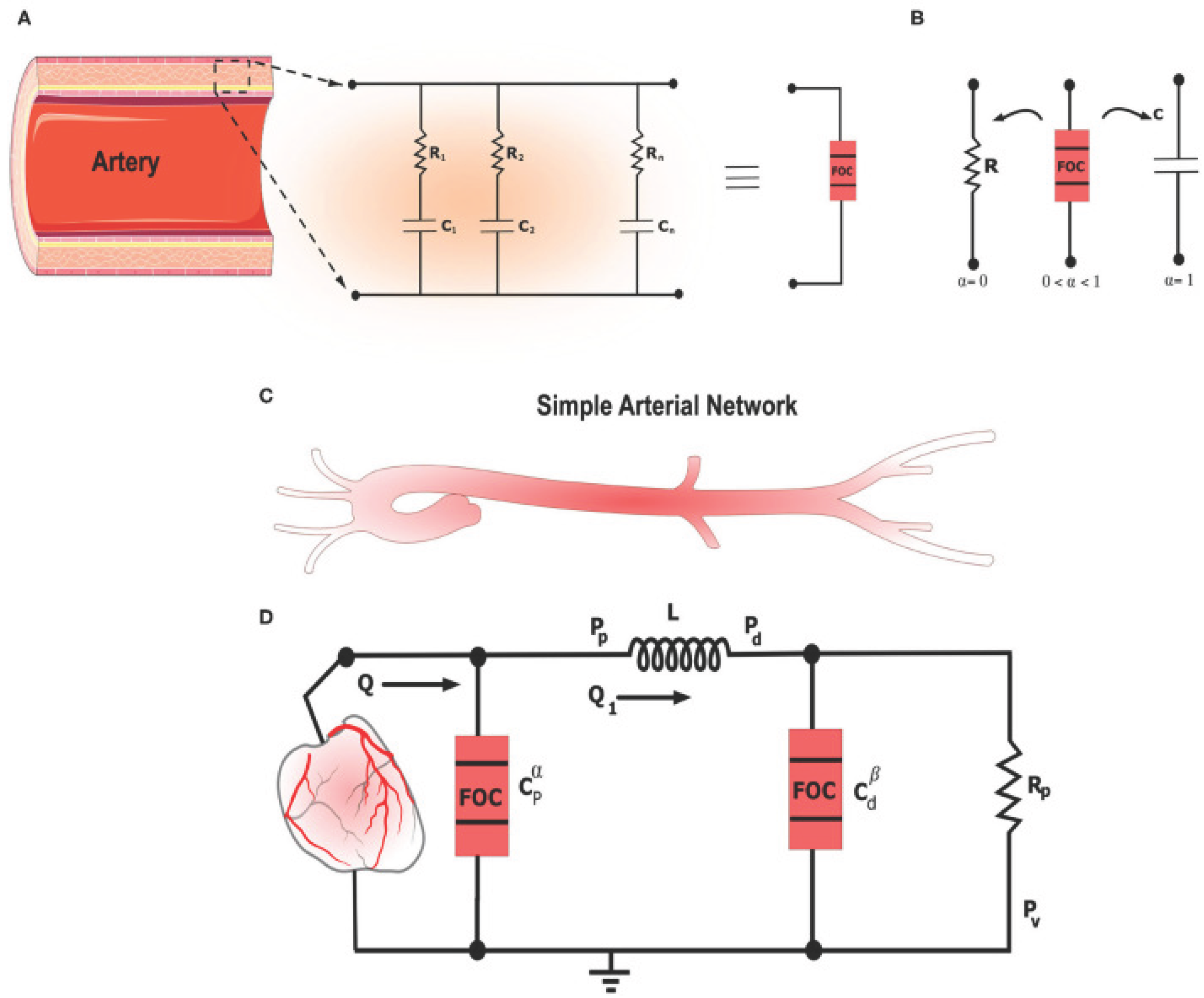
Figure 2.
Approximate solutions for: (1-1) TCFKE in Example (1) with and different values of ; (1-2) MTCFKE in Example (2) with , , .
Figure 2.
Approximate solutions for: (1-1) TCFKE in Example (1) with and different values of ; (1-2) MTCFKE in Example (2) with , , .
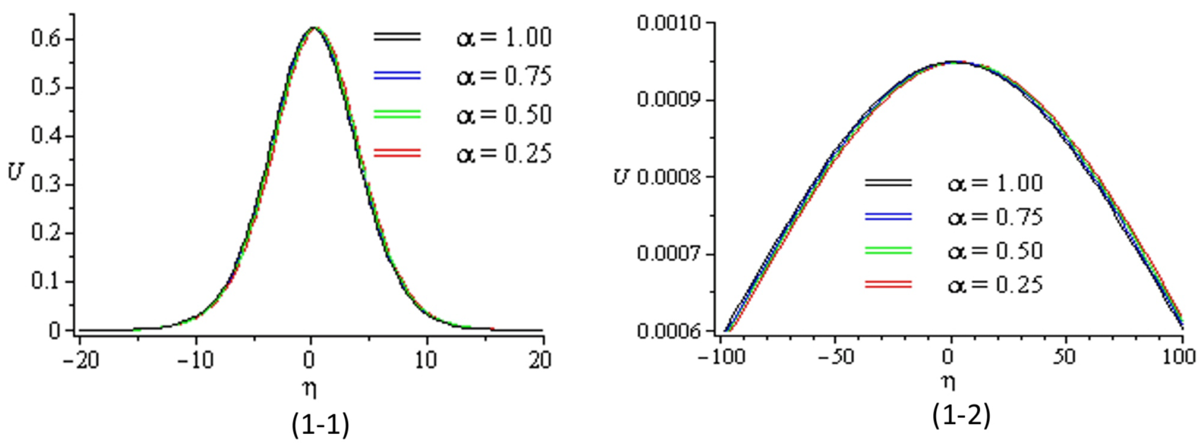
Figure 3.
OAFM solutions for: (2-1) TCFKE in Example (1) with and different values of ; (2-2) MTCFKE in Example (2) with , , .
Figure 3.
OAFM solutions for: (2-1) TCFKE in Example (1) with and different values of ; (2-2) MTCFKE in Example (2) with , , .
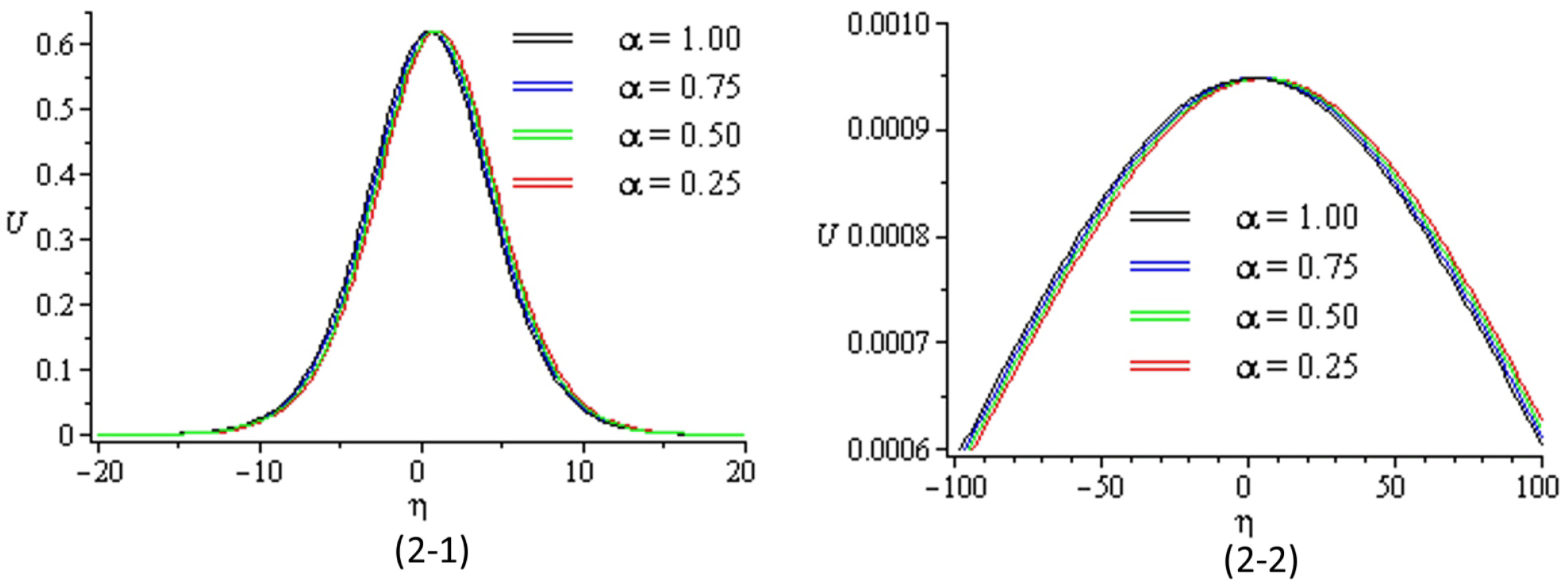
Figure 4.
OAFM solutions for: (3-1) TCFKE in Example (1) with and different values of ; (3-2) MTCFKE in Example (2) with , , .
Figure 4.
OAFM solutions for: (3-1) TCFKE in Example (1) with and different values of ; (3-2) MTCFKE in Example (2) with , , .
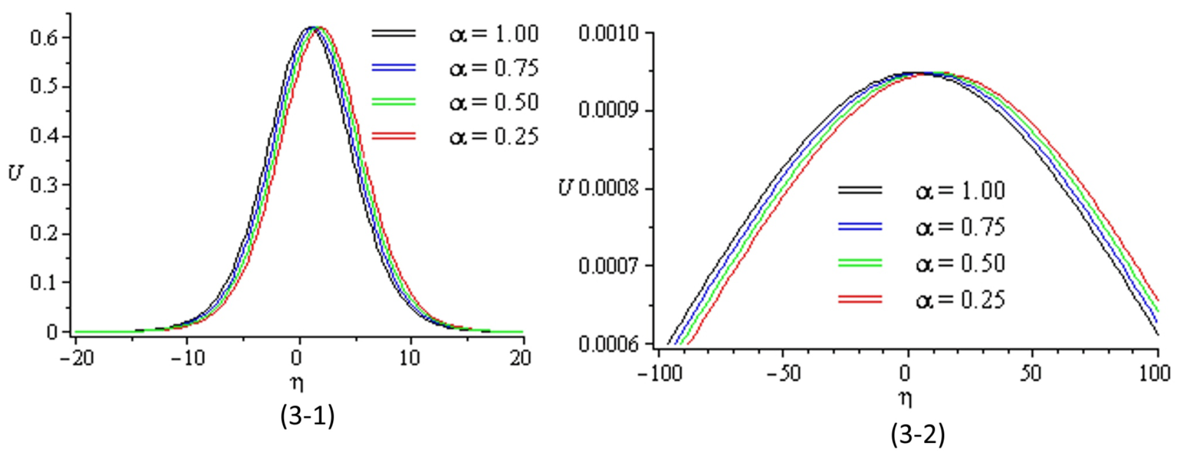
Figure 5.
Plot of OAFM solutions for TCFKE in Example (1) and MTCFKE in Example (2) with , , .
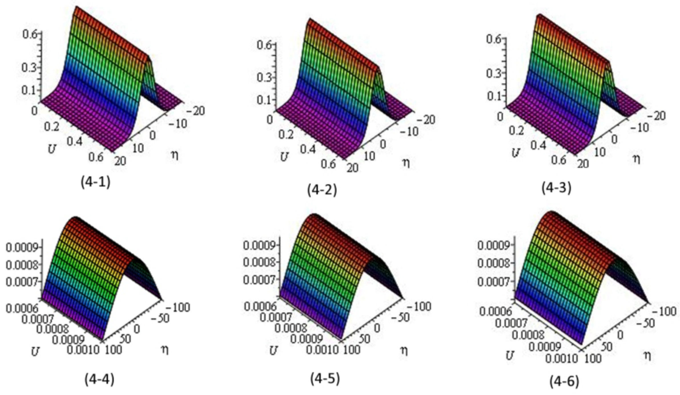
Figure 6.
Plot of OAFM solutions for TCFKE in Example (1) and MTCFKE in Example (2) with , , .
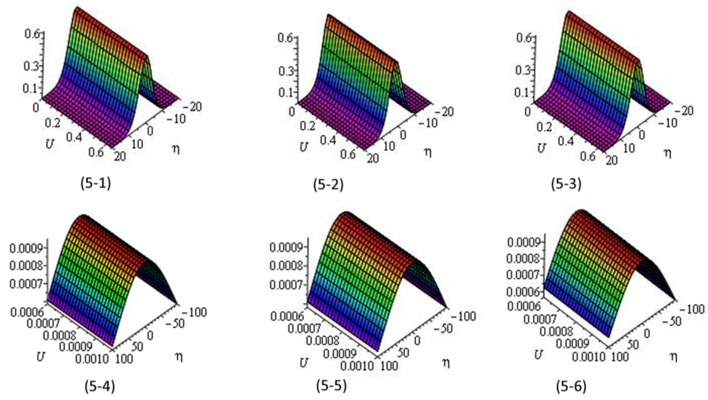
Figure 7.
Surface plot of approximate solutions for TCFKE in Example (1) and MTCFKE in Example (2) with , , .
Figure 7.
Surface plot of approximate solutions for TCFKE in Example (1) and MTCFKE in Example (2) with , , .
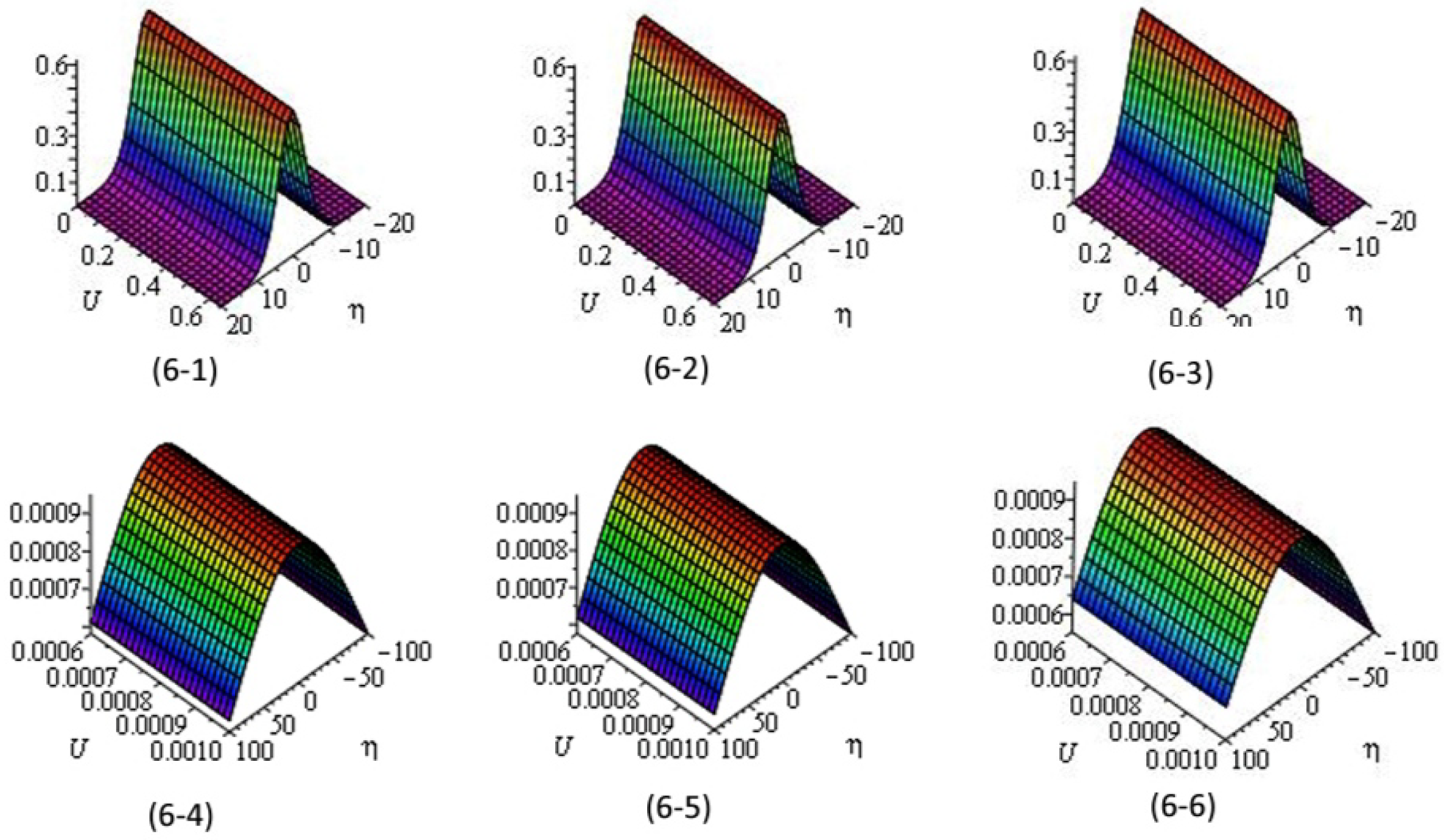
Figure 8.
Plot of OAFM solutions for TCFKE in Example (1) and MTCFKE in Example (2) with , , .
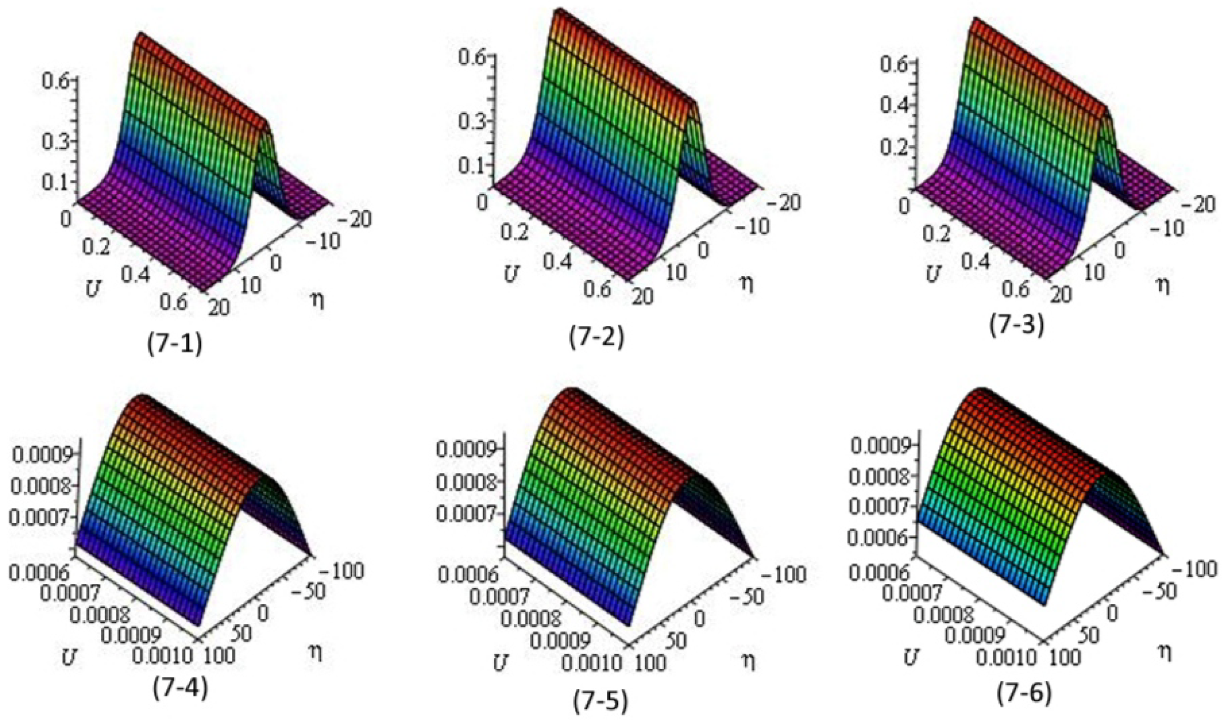

Table 1.
Absolute error of OAFM at and with different values of in Example (1).
| AE(OAFM) | AE(NTDM)[40] | AE(RPSM) [39] | |
| 0 | 0 | 0 | |
Table 2.
Approximate solutions for TCFKE at with different values of and in Example (1).
| OAFM | NTDM [40] | RPSM [39] | ||
| 1 | ||||
Disclaimer/Publisher’s Note: The statements, opinions and data contained in all publications are solely those of the individual author(s) and contributor(s) and not of MDPI and/or the editor(s). MDPI and/or the editor(s) disclaim responsibility for any injury to people or property resulting from any ideas, methods, instructions or products referred to in the content. |
© 2025 by the authors. Licensee MDPI, Basel, Switzerland. This article is an open access article distributed under the terms and conditions of the Creative Commons Attribution (CC BY) license (http://creativecommons.org/licenses/by/4.0/).
Copyright: This open access article is published under a Creative Commons CC BY 4.0 license, which permit the free download, distribution, and reuse, provided that the author and preprint are cited in any reuse.


