
Submitted:
03 March 2025
Posted:
04 March 2025
You are already at the latest version
Abstract
In this study, we extend the Simple Equations Method (SEsM) and adapt it for finding exact solutions of systems of fractional nonlinear partial differential equations (FNPDEs). In accordance with the extended SEsM, the analytical solutions to the studied FNPDEs are constructed as complex composite functions which combine two single composite functions, comprising power series of solutions of two simple equations or two special functions. The novel and innovative aspect of the proposed extended methodology is that the simple equations or the special functions used have different independent variables (different wave coordinates). In this context, the proposed approach is mostly suitable for application to systems of FNPDEs (or NPDEs) that describe the complex wave dynamics of real processes in different scientific fields such as fluid mechanics, plasma physics, optics, etc. The extended SEsM is applied to the time–fractional Boussinesq-like system, assuming that each system variable supports multi-wave dynamics, which involves the combined propagation of two distinct waves traveling at different wave speeds. As a result, numerous complex multi-wave solutions including combinations of different hyperbolic, elliptic and trigonometric functions are derived. In order to visualize the complex wave dynamics obtained through the applied analytical approach, some analytical solutions have been numerically simulated.
Keywords:
Extended Simple Equation Method
; time–fractional Boussinesq–like system
; analytical solutions
; numerical simulations
MSC: 35A24; 35G50
1. Introduction
Over the past two decades, the fractional nonlinear partial differential equations (FNPPDEs) have gained considerable popularity in the scientific community for modeling and analyzing a wide range of phenomena observed in the real world. This efficient framework allows for more accurately reproducing the complex wave dynamics of model systems encountered in diverse fields such as biology and ecology [1]–3], fluid dynamics [4]–7], finance and economics [8]–10], engineering [11]–13], among others. These systems often exhibit features such as memory effects, spatial heterogeneity and nonlocal interactions that integer-order models fail to adequately address. One approach to better understand this unconventional dynamic behavior is to find analytical solutions to the such models and their expert analysis. Finding exact solutions to FNPDEs, unlike those of NPDEs, is more difficult due to the necessary combination of elements from nonlinear dynamics with those arising from the fractional derivative’s order.
To date, two main approaches to finding exact and approximate analytical solutions of FNPDEs dominate the scientific literature: (1) Using fractional transformations, which allow reducing the studied NFPDEs to integer order nonlinear ODEs. Then, various well–known approaches from the ODE theory can be applied to the latter to obtain exact general and particular solutions of NPDEs. The most famous and applied methodologies in this direction use the so–called ansatz techniques [14]. Based on ansatz techniques, numerous analytical methods have been developed, including the Hirota method [15], the homogeneous balance method [16], the auxiliary equation method [17], the Jacobi elliptic function expansion method [18], the (G′/G)-expansion method [19], the F–expansion method [20], the tanth–function method [21], the first integral method [22], the exponential function method [23], the simplest equation method [24], the modified method of simplest equation [25]–27], etc. There are also numerous studies that apply these methods to find analytical solutions to various single NPDEs and systems of NPDEs. The SEsM, used in this study, is a relatively new methodology [28,29]. It is an extension of the Modified Method of Simple Equation, and has an almost universal nature. This is because most of the above–mentioned methods in this category are its particular cases, as proven in [30,31,32,33]; (2) Using standard traveling wave transformations, which allow reducing the studied FNPDEs to simpler fractional PDEs or fractional ODEs, whose analytical solutions are known (For instance, see Ref. [34]). Then, similarly to the first approach, analytical solutions of the studied FNPDEs are constructed on the basis of known analytical solutions of fractional ODEs. Among the methods in this category, the most widely used is so called fractional sub–equation method [35,36,37,38]. This method is based on known solutions of the fractional ODE of Riccati and its sub–variants. Another popular method in this category is the fractional elliptic Jacobi equation method [39,40], which uses Jacobi elliptic functions to derive analytical solutions of the studied FPDEs. When using the second approach, the Mittag–Leffler functions often appear in solutions of the studied FNPDEs, because they effectively describe the behavior of systems with fractional order.
The extended SEsM used in the current study follows the first approach, above given. In detail, we shall adapt the SEsM [41]–44], which is established for finding exact solutions of integer–order NPDEs to find exact solutions of a known system of FNPDEs by introducing an appropriate fractional transformation. The new and different emphasis in this methodology is that the solutions of the studied equations are presented as complex composite functions, including series of solutions of two (or more) simple equations or two (or more) special functions. In addition, we extend the current version of the SEsM by assuming that the simple equations used have different independent variables. The latter is a new approach that firstly has been applied to find analytical solutions of the extended integer–order KDV equation [45]. Numerous traveling wave solutions have been derived in [45] using an ODE of Abel, an ODE of Bernoulli, an ODE of Riccati and its sub–variants. Later, in [46], the authors independently proposed a similar methodology based on the extended Kudryashov method, as it was applied to find exact solutions of an integer-order Boussinesq-like system and the integer-order shallow-water wave equation. To obtain exact analytical solutions of the aforementioned models, the authors in [46], used two sub–variants of the ODE of Riccati as simple equations. In terms of finding exact solutions to systems of FNPDEs, a similar version of the extended SEsM was applied in [47,48] to dynamical models describing natural processes in fluid mechanics and ecology. In these studies, the obtained traveling wave solutions were presented by sums of two single composite functions containing the solutions of two distinct simple equations with the same independent variable. In [49,50], another version of the extended SEsM was applied to an extended variant of a popular ecological system of FNPDEs. In these studies, the obtained analytical solutions of the studied system are presented by distinct single composite functions with different independent variables (different wave coordinates) for each system variable.
In this study we shall apply the extended SEsM to the time–fractional version of the Boussinesq–like system [51]
where is the elevation of a water wave and is the surface velocity of water along x-direction, is a time–fractional number and k is a coefficient, related to the depth of water. For the case , Equation (1) reduces to the classical Boussinesq system. Equation (1) is a very useful model for coastal and civil engineering in predicting the propagating nonlinear water waves in harbour and coastal zones.
Following the extended SEsM algorithm given bellow, we shall search for analytical solutions of Equation (1) in more specific manner taking into account the special wave characteristics of the studied time–fractional Boussinesq model. It is known that most fluid systems exhibit simultaneously nonlinear and dispersive properties. These distinct properties support diverse wave modes like solitary waves, periodic waves, and dispersive wave trains. In addition, variation in wave speeds of the distinct waves can be appeared due to factors such as the dispersion relation and the nonlinear interactions. Thus, such systems can demonstrate multi–scale dynamics, involving fast and slow wave components in accordance with its dispersion and nonlinear components. Taking into account these arguments, bellow we shall present the analytical solutions for each system variable of Equation (1) as a composition of two single composite functions with different wave coordinates. These composite functions contain power series of solutions of two distinct simple equations. We hope that such a presentation of the aforementioned solutions provides more accurate and insightful depiction of the complex behaviors inherent in the studied fluid system.
2. Preliminaries
In this section we present several important definitions of the modified Riemann-Liouville derivatives that we will use in the current study. These definitions are stated according to the basic results obtained by G. Jumarie in [52]–54]
2.1. Fractional derivative via fractional difference
Definition 2.1. Let , denote a continuous (but not necessarily differentiable) function, and let denote a constant discretization span. Define the forward operator by the equality (the symbol means that the left side is defined by the right side)
then the fractional difference of order , , of is defined by the expression
and its fractional derivative of order is defined by the limit
2.2. Modified fractional Riemann–Liouville derivative
Definition 2.2. Refer to the function of Definition 2.1.
(i) Assume that is a constant K . Then its fractional derivative of order is
(ii) When is not a constant, then we will set
and its fractional derivative will be defined by the expression
in which, for negative , one has
whilst for positive , we will set
When ,
In order to find the fractional derivative of compound functions, the following equation holds:
2.3. Taylor’s series of fractional order
Definition 2.3. The continuous function has a fractional derivative of order . For any positive integer k and for any , , then the following equality holds
where .
Definition 2.4. If , then
or, if , then
3. Description of the Generalized SEsM Algorithm
In this section, we present the generalized algorithm of a specific version of SEsM, exposing all the possibilities it provides for obtaining various complex analytical solutions to systems of FNPDEs (or single FNPDEs), depending on the selected fractional transformation and simple equation’s types used by the implementer. As it is demonstrated below, unlike the original SEsM algorithm outlined in [41]–43], we have swapped its first and second steps, incorporating methodological extensions into both steps of the original SEsM algorithm. In addition, the proposed SEsM algorithm presented below covers both approaches to the chosen traveling wave transformation discussed earlier in the paper. Our goal is to allow the user to choose which of the two approaches to use when extracting exact solutions to systems of FNPDEs similar to Equation (1).
Taking into account the problem we set out to solve in this study, we shall demonstrate all the possible steps of the algorithm above mentioned for a system of two NPPDEs with two independent variables:
where D denotes the arbitrary fractional order derivative operator, as superscripts give its fractional number and subscripts denote time and partial derivatives. Here, and are polynomials of u and v and their derivatives, respectively, where and are unknown functions.
Remark: We note that the variant of SEsM presented below is suitable to be applied mainly to real-world dynamical models of the type (15), where the system variables are expected to exhibit complex synchronized multi–layered wave behavior.
The generalized extended SEsM algorithm which is adopted for finding exact solutions of FNPDEs includes the following basic steps:
- 1.
-
Construction of the solutions of Equation (15). The solution of Equation (15) can be constructed as a complex composite function of two or more single composite functions, involving solutions of two or more simple equations with different independent variables. There are many variants of combination between the single composite function in constructing the corresponding solution, but below we will present only a few of its simplest forms:Variant 1:Variant 2:Variant 3:whereas and are solutions of simple equations , which are presented in Step 3 of the SEsM algorithm.
- 2.
-
Selection of the traveling wave type transformation. To apply the SEsM to Equation (15), it is crucial to define the fractional derivatives in those equations. The choice of fractional derivatives (e.g., Riemann-Liouville, Caputo, conformable, etc) is essential for accurately modeling wave dynamics and reflecting the system’s physical properties, based on factors like the process nature, boundary conditions, and memory effects interpretation. In this context, the following variants of transformations are possible:
-
Variant 1: Use a fractional transformation. The choice of explicit form of the fractional traveling wave transformation depends on how the fractional derivatives in Equation (15) are defined. Bellow, the most used fractional traveling wave transformations are selected:– Conformable fractional traveling wave transformation: , defined for conformable fractional derivatives [55];– Fractional complex transform: , defined for modified Riemann–Liouville fractional derivatives [52], which can applied for Caputo fractional derivatives and other fractional derivative types in studied FNPDEs [56].In the both cases, the studied FNPDEs are reduced to integer–order nonlinear ODEs.
- Variant 2: Use a standard traveling wave transformation. In this case, by introducing a traveling wave ansatz in the selected variant solutions from Step 1, the studied FNPDEs are reduced to fractional nonlinear ODEs.
-
- 3.
-
Selection of the forms of the used simple equations.
-
For Variant 1 of Step 2: The general form of the integer–order simple equations used is:By fixing and (at ) in Equation (20), different types integer–order ODEs can be used as simple equations, such as:– ODEs of first order with known analytical solutions (For example, an ODE of Riccati, an ODE of Bernoulli, an ODE of Abel of first kind, an ODE of tanh–function, etc);– ODEs of second order with known analytical solutions (For example, elliptic equations of Jaccobi and Weiershtrass and their sub–variants, an ODE of Abel of second kind, etc.). This scenario can be applied to specific classes FNPDEs (or NPDEs) (For instance, see [57]).
-
For Variant 2 of Step 2: The general form of the fractional simple equations used is:By fixing and in Equation (21), different types fractional ODEs can be used as simple equations, such as a fractional ODE of Riccati, a fractional ODE of Bernoulli or other polynomial or elliptic form equations, which solutions are available in the literature.
-
- 4.
- Derivation of the balance equations and the system of algebraic equations. The fixation of the explicit form of solutions of Equation (15) presented in Step 1 of the SEsM algorithm depends on the balance equations derived. Substitutions of the selected variants from Steps 1,2 and 3 in Equation (15) leads to obtaining polynomials of the functions and . The coefficients in front of these functions include the coefficients of the solution of the considered FNPDEs as well as the coefficients of the simple equations used. Analytical solutions of Equation (15) can be extracted only if each coefficient in front of the functions and contains almost two terms. Equating these coefficients to zero leads to formation of a system of nonlinear algebraic equations for each variant chosen according Steps 1,2 and 3 of the SEsM algorithm.
- 5.
- Derivation of the analytical solutions. Any non–trivial solution of the algebraic system above mentioned leads to a solution of the studied FNPDEs by replacing the specific coefficients in the corresponding variant solutions, given in Step 1 as well as by changing the traveling wave coordinates chosen by the variants given in Step 2. For simplicity, these solutions are expressed through special functions. For a Variant 1 of the Step 3, these special functions are and , as their explicit forms are determined on the basis of the specific form of the simple equations chosen (For reference, see Equation (20)). For a Variant 2 of the Step 3, the special functions are and , whose exact forms are determined by the type of fractional simple equations used (For reference, see Equation (21)).
In this study, we shall demonstrate only some of the possibilities provided by the generalized SEsM algorithm, presented above, by applying only one of its variants to Equation (1).
4. Exact Solutions of the Time Fractional Boussinesq–Like System Using a Fractional Wave Transformation
According to the generalized SEsM algorithm, presented above, we choose to present the general solution of Equation (1) by Equation (16) in the way:
In view of the studied shallow water problem, we choose to present the memory effects occurring in the system (1) in sense of modified Riemann–Liouville fractional derivatives, presented in Section 2. Thus, the fractional transformations take the form:
The balance equations are and . Substitution of Equations (22)–(24) in Equation (1) leads to a system of nonlinear equations. There are many variants and sub–variants of Equation (24) depending on the numerical values of their coefficients. For each of these variants or sub–variants, there are specific solutions, which are available in the literature. Below, we shall present only a few examples of specific sub–variants of simple equations of type (24). For example, as a starting point, we shall choose to use the first simple equation of Equation (24) in its complete form with respect to the coefficients , i.e. . Regarding to the second simple equation of (24), however, we shall chose to use its simplest sub–variant, where . Then, the system of nonlinear algebraic equations is:
In the rest of this article, we shall present only a part of off-beat possible solutions which can be derived on dependence of the numerical values of the coefficients in polynomial parts of Equation (24) for this specific case.
4.1. Case 1: When and in Equation (24)
We present the general solution of Equation (1) by special functions in the following manner:
For this specific case, several families of solutions of Equation (1) can be obtained depending on numerical values of the coefficients and .
4.1.1. Variant 1: When and in Equation (26)
Let us consider the case, where and in Equation (26). Then, Equation (27) reduces to
where the special function is a particular solution of an ODE of second order, given in [57,58], and the special function presents particular solutions of an ODE of second order, which can be found in [59].
We solve the algebraic system (25) by fixing . Many solutions of the system (25) can be derived, but we aim to find those solutions, where the coefficients are free parameters. In this way, one non–trivial solution of this system is:
According to all possible variant solutions , the following families of solutions (28) of Equation (1) are possible:
where [57]
and [59]
In Equation (36), and are arbitrary constants. In all the solutions provided in this subsection, .
4.1.2. Variant 2: When and in Equation (26)
In this specific case, the solution of Equation (1) is reduced to:
where is presented in Equation (31) and is a particular solution of an ODE of second order, given in [60].
In Equation (38), .
4.1.3. Variant 3: When and in Equation (26)
In this specific case, the solution of Equation (1) is reduced to:
where is presented in Equation (31) and is a particular solution of an ODE of second order, given in [57,58].
In Equation (41), .
4.2. Case 2: When and in Equation (24)
We present the general solution of Equation (1) by special functions in the following manner:
In Equation (44), we choose to express the special function (the solutions of the first equation in (43)), in terms of Weierstrass–elliptic functions [61].The special function presents the same solutions, as those given in the previous section. Depending on variant solutions and , various families of solutions of Equation (1) can be selected.
4.2.1. Variant 1. When and in Equation (43)
One non–trivial solution of the algebraic system (25) at and , including the coefficients and as free parameters, is:
Then, substitution of Equation (45) in Equation (44) leads to the following solutions of Equation(1):
where
and is presented in Equation (32).
where is presented in Equation (47) and is presented in Equation (34).
where is presented in Equation (47) and is presented in Equation (36).
where
and is presented in Equation (32).
where is presented in Equation (51) and is presented in Equation (34).
where is presented in Equation (51) and is presented in Equation (36).
where
and is presented in Equation (32).
where is presented in Equation (55) and is presented in Equation (34).
where is presented in Equation (55) and is presented in Equation (36).
where
and is presented in Equation (32).
where is presented in Equation (59) and is presented in Equation (34).
where is presented in Equation (59) and is presented in Equation (36).
where
and is presented in Equation (32).
where is presented in Equation (63) and is presented in Equation (34).
where is presented in Equation (63) and is presented in Equation (36).
where
and is presented in Equation (32).
where is presented in Equation (67) and is presented in Equation (34).
where is presented in Equation (67) and is presented in Equation (36). In all the solutions, presented in this subsection,
4.2.2. Variant 2: When and in Equation (43)
When , Equation (45) is reduced to:
Substitution of Equation (70) in the particular variant of Equation (44) leads to the following solutions of Equation (1):
where is presented in Equation (47), and is presented in Equation (39).
where is presented in Equation (51), and is presented in Equation (39).
where is presented in Equation (55), and is presented in Equation (39).
where is presented in Equation (59), and is presented in Equation (39).
where is presented in Equation (63), and is presented in Equation (39).
where is presented in Equation (67), and is presented in Equation (39). In all the solutions presented in this subsection, .
4.2.3. Variant 3: When and in Equation (43)
When , Equation (45) is reduced to:
Substitution of Equation (77) in the particular variant of Equation (44) leads to the following solutions of Equation (1):
where is presented in Equation (47) and is presented in Equation (42).
where is presented in Equation (51) and is presented in Equation (42).
where is presented in Equation (55) and is presented in Equation (42).
where is presented in Equation (59) and is presented in Equation (42).
where is presented in Equation (63) and is presented in Equation (42).
where is presented in Equation (67) and is presented in Equation (42). In all the solutions, presented in this subsection, .
For all analytical and numerical calculations in this article, we use the computational software Maple (https://www.maplesoft.com).
5. Numerical Simulations
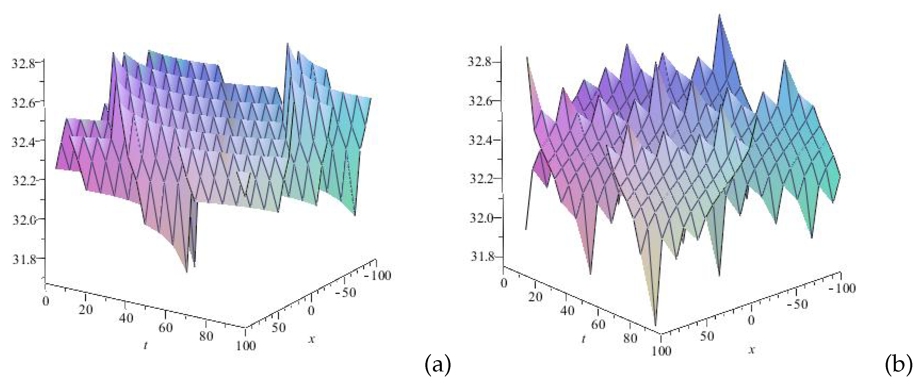
In this section, we present visualizations of some analytical solutions presented in Section 4. In accordance with the obtained exact solutions of Equation (1), which are combinations of various special functions, Figure 1, Figure 2, Figure 3, Figure 4, Figure 5, Figure 6, Figure 7, Figure 8 and Figure 9 illustrate combinations of different type’s waves, propagating in the studied water medium. It is obvious that Equation (1) demonstrates complex wave behavior, which can vary significantly depending on the specific exact solution. Here, we have shown the more interesting variants of mixed waves, trying to summarize them briefly depending on their wave type. For example, in the simplest case, one can observe combinations of waves of one type, such as single solitons (Figure 1) or complex multi-soliton structures (Figure 3) with different amplitudes and wavelengths. A more complex scenario involves the propagation of soliton wave packets combined with single solitons, as shown in Figure 4 and Figure 7. Of particular interest are combinations of synchronized kink and anti-kink waves and periodic structures (Figure 2 and Figure 5 ), as well as kink and anti-kink wave packets combined with multiple single solitons of different amplitude and wavelength (Figure 6 and Figure 8). The complex wave dynamics of the system (1) is also demonstrated in Figure 9, where combinations of kinks, anti-kinks, and multi–soliton wave packets are observed. We note, that the multi-wave behavior of the system (1), based on any analytical solution, presented in this section, can change qualitatively depending on the choice of the numerical values of the coefficients in it, the fractional derivative order, as well as the time and spatial numerical intervals of the plots. In this context, a more realistic picture of the wave dynamics of the studied system for prediction or control purposes can only be obtained if numerical values or numerical intervals of the above-mentioned parameters are specified.
6. Conclusions
In this study, we have proposed an extended version of the SEsM, which is applicable for obtaining analytical solutions of FNPDEs (in particular, NPDEs), that model dynamics of real-world processes with complex wave behavior. The solutions to such NPDEs are expressed as combinations of single composite functions, which involve solutions to two distinct simple equations or two distinct special functions with different independent variables. A generalized algorithm of the methodology has been presented, allowing the researcher to flexibly choose an appropriate traveling wave transformation and appropriate simple equations’ types to extract exact solutions to the studied models. This highlights the universality of the method in its application to both systems of FNPDEs and single FNPDEs of various types.
One variant of the extended SEsM has been applied to the time-fractional Boussinesq–like system, introducing a fractional traveling wave transformation and utilizing two second-order ODEs with different coordinates in their generalized form as simple equations. It has been demonstrated, that for different numerical values of the coefficients in polynomial parts of these equations, they reduce to various forms, each yielding distinct analytical solutions. By different combinations of these solutions, we have derived a part of the possible analytical solutions to the studied system of FNPDEs, including diverse combinations of hyperbolic, elliptic, and trigonometric functions. In this way, the investigated water medium exhibits a variety of mixed waves, such as single solitons, multi-solitons with different amplitudes and wavelengths, complex kink and anti-kink structures, and periodic wave packets. The propagation of different types of waves in the studied medium, analytically and numerically illustrated in this paper, is explained by the interplay of nonlinear interactions and dispersion effects present in Equation (1).
It is important to note, that the analytical solutions obtained in this study, present only a a part of the possible solutions under the selected simple equations (24). For instance, the solutions of Jacobi elliptic equation, along with its hyperbolic and trigonometric analogues, or the solutions of the Abel equation of second kind, could also be used in extracting the solutions of Equation (1). Additionally, the construction solutions to Equation (1) can incorporate also combinations of series of known solutions of different ODEs of first order, or mixture combinations of series of known solutions of ODEs of first order and ODEs of second order. Following another variant of the extended SEsM, proposed in [50], it is also feasible to construct the solution of Equation (1) by distinct single composite functions that include series of solutions of two distinct simple equations with different independent variables for each system variable. These ideas, however, will be the subject of our furture investigations.
Funding
E. V. Nikolova tanks the project “Artificial intelligence for investigation and modeling of real processes”, KP-06-H82/4, funded by the Bulgarian National Science Fund, for its financial support.
References
- Rivero, M.; Trujillo, J.J.; Vázquez, L.; Velasco, M.P. Fractional dynamics of populations. Appl. Math. Comput. 2011, 218, 1089–1095. [Google Scholar] [CrossRef]
- Owolabi, K.M. High-dimensional spatial patterns in fractional reaction-diffusion system arising in biology. Chaos Solitons Fractals 2020, 134, 109723. [Google Scholar] [CrossRef]
- Ghanbari, B.; Günerhan, H.; Srivastava, H.M. An application of the Atangana-Baleanu fractional derivative in mathematical biology: A three-species predator-prey model. Chaos Solitons Fractals 2020, 138, 109910. [Google Scholar] [CrossRef]
- Kulish, V.V.; Lage, J.L. Application of fractional calculus to fluid mechanics. J. Fluids Eng. 2002, 124, 803–806. [Google Scholar] [CrossRef]
- Yıldırım, A. Analytical approach to fractional partial differential equations in fluid mechanics by means of the homotopy perturbation method. Int. J. Numer. Methods Heat Fluid Flow 2010, 20, 186–200. [Google Scholar] [CrossRef]
- Hosseini, V.R.; Rezazadeh, A.; Zheng, H.; Zou, W. A nonlocal modeling for solving time fractional diffusion equation arising in fluid mechanics. Fractals 2022, 30, 2240155. [Google Scholar] [CrossRef]
- Ozkan, E.M. New Exact Solutions of Some Important Nonlinear Fractional Partial Differential Equations with Beta Derivative. Fractal Fract. 2022, 6, 173. [Google Scholar] [CrossRef]
- Fallahgoul, H.; Focardi, S.; Fabozzi, F. Fractional Calculus and Fractional Processes with Applications to Financial Economics: Theory and Application; Academic Press: Cambridge, MA, USA, 2016. [Google Scholar]
- Ara, A.; Khan, N.A.; Razzaq, O.A.; Hameed, T.; Raja, M.A.Z. Wavelets optimization method for evaluation of fractional partial differential equations: An application to financial modelling. Adv. Differ. Equ. 2018, 2018, 8. [Google Scholar] [CrossRef]
- Tarasov, V.E. On history of mathematical economics: Applicatioactionaln of fr calculus. Mathematics 2019, 7, 509. [Google Scholar] [CrossRef]
- Kumar, S. A new fractional modeling arising in engineering sciences and its analytical approximate solution. Alex. Eng. J. 2013, 52, 813–819. [Google Scholar] [CrossRef]
- Sun, H.; Zhang, Y.; Baleanu, D.; Chen, W.; Chen, Y. A new collection of real world applications of fractional calculus in science and engineering. Commun. Nonlinear Sci. Numer. Simul. 2018, 64, 213–231. [Google Scholar] [CrossRef]
- Chen, W.; Sun, H.; Li, X. Fractional Derivative Modeling in Mechanics and Engineering; Springer Nature: Berlin/Heidelberg, Germany, 2022. [Google Scholar]
- Anco, S. C.; Liu, S. Exact solutions of semilinear radial wave equations in n dimensions. Journal of Mathematical Physics, 2003, 44(9), 4103–4117. [CrossRef]
- Hirota, R. Hirota, R. Exact Solution of the Korteweg-de Vries Equation for Multiple Collisions of Solitons. Physical Review Letters, 1971, 27(18), 1192–1194. [CrossRef]
- Wang, M.; Zhou, Y. The Homogeneous Balance Method and Its Application to Nonlinear Equations. Chaos, Solitons & Fractals, 1996, 7(12), 2047–2054. [CrossRef]
- Liu, S. K.; Fu, Z. T.; Liu, S. D.; Zhao, Q. Jacobi Elliptic Function Expansion Method and Periodic Wave Solutions of Nonlinear Wave Equations. Physics Letters A, 2001, 289(1-2), 69–74. [CrossRef]
- Kudryashov, N.A. Exact soliton solutions of the generalized evolution equations of wave dynamics. Journal of Applied Mathematics and Mechanics 1988, 55, 372–375. [Google Scholar] [CrossRef]
- Wang, M.; Li, X.; Zhang, J. The (G′/G)-expansion method and travelling wave solutions of nonlinear evolution equations in mathematical physics. Phys. Lett. A 2008, 372, 417–423. [Google Scholar] [CrossRef]
- Zhang, J.; Li, Z. The F–expansion method and new periodic solutions of nonlinear evolution equations. Chaos, Solitons & Fractals 2008, 37, 1089–1096. [Google Scholar]
- Wazwaz, A. M. The tanh method for traveling wave solutions of nonlinear equations. Appl. Math. Comput. 2004, 154, 713–723. [Google Scholar] [CrossRef]
- Feng, Z. The First Integral Method to Study the Burgers–KdV Equation. Journal of Physics A: Mathematical and General 2002, 35, 343–349. [Google Scholar] [CrossRef]
- He, J. H.; Wu, X. H. Exp-Function Method for Nonlinear Wave Equations. Chaos, Solitons & Fractals, 2006, 30(3), 700–708. [CrossRef]
- Kudryashov, N. A. Simplest Equation Method to Look for Exact Solutions of Nonlinear Differential Equations. Chaos, Solitons & Fractals, 2005, 24(5), 1217–1231. [CrossRef]
- Vitanov, N.K. On modified method of simplest equation for obtaining exact and approximate solutions of nonlinear PDEs: The role of the simplest equation. Commun. Nonlinear Sci. Numer. Simul. 2011, 16, 4215–4231. [Google Scholar] [CrossRef]
- Vitanov, N.K. Application of Simplest Equations of Bernoulli and Riccati Kind for Obtaining Exact Traveling-Wave Solutions for a Class of PDEs with Polynomial non-linearity. Commun. Non-Linear Sci. Numer. Simul. 2010, 15, 2050–2060. [Google Scholar] [CrossRef]
- Vitanov, N.K. Modified Method of Simplest Equation: Powerful Tool for Obtaining Exact and Approximate Traveling-Wave Solutions of non-linear PDEs. Commun. Non-Linear Sci. Numer. Simul. 2011, 16, 1176–1185. [Google Scholar] [CrossRef]
- Vitanov, N.K. Recent Developments of the Methodology of the Modified Method of Simplest Equation with Application. Pliska Stud. Math. Bulg. 2019, 30, 29–42. [Google Scholar]
- Vitanov, N.K. Modified Method of Simplest Equation for Obtaining Exact Solutions of non-linear Partial Differential Equations: History, recent development and studied classes of equations. J. Theor. Appl. Mech. 2019, 49, 107–122. [Google Scholar] [CrossRef]
- Vitanov, N.K.; Dimitrova, Z.I.; Vitanov, K.N. Simple Equations Method (SEsM): Algorithm, Connection with Hirota Method, Inverse Scattering Transform Method, and Several Other Methods. Entropy 2021, 23, 10. [Google Scholar] [CrossRef]
- Vitanov, N.K. The Simple Equations Method (SEsM) For Obtaining Exact Solutions Of non-linear PDEs: Opportunities Connected to the Exponential Functions. AIP Conf. Proc. 2019, 2159, 030038. [Google Scholar] [CrossRef]
- Dimitrova, Z.I.; Vitanov, K.N. Homogeneous Balance Method and Auxiliary Equation Method as Particular Cases of Simple Equations Method (SEsM). AIP Conf. Proc. 2021, 2321, 030004. [Google Scholar] [CrossRef]
- Dimitrova, Z.I. On several specific cases of the simple equations method (SEsM): Jacobi elliptic function expansion method, F-expansion method, modified simple equation method, trial function method, general projective Riccati equations method, and first intergal method. AIP Conf. Proc. 2022, 2459, 030006. [Google Scholar] [CrossRef]
- Vitanov, N.K. Simple equations method (SEsM) and nonlinear PDEs with fractional derivatives. AIP Conf. Proc. 2022, 2459, 030040. [Google Scholar] [CrossRef]
- Zhang, S.; Zhang, H-Q. Fractional sub-equation method and its applications to nonlinear fractional PDEs. Phys. Lett. A 2011, 375, 1069–1073. [Google Scholar] [CrossRef]
- Guo, S.; Mei, L.; Li, Y.; Sun, Y. The improved fractional sub-equation method and its applications to the space-time fractional differential equations in fluid mechanics. Phys. Lett. A 2012, 376, 407–411. [Google Scholar] [CrossRef]
- Lu, B. Backlund transformation of fractional Riccati equation and its applications to nonlinear fractional partial differential equations. Phys. Lett. A, 2012, 376, 2045–2048. [Google Scholar] [CrossRef]
- Zheng, B.; Wen, C. Exact solutions for fractional partial differential equations by a new fractional sub-equation method. Adv. Differ. Equ. 2013, 2013, 199. [Google Scholar] [CrossRef]
- Zheng, B. A new fractional Jacobi elliptic equation method for solving fractional partial differential equations. Adv. Differ. Equ. 2014, 2014, 228. [Google Scholar] [CrossRef]
- Feng, Q.; Meng., F. Explicit solutions for space-time fractional partial differential equations in mathematical physics by a new generalized fractional Jacobi elliptic equation-based sub-equation method. Optik 2016, 127, 7450–7458. [Google Scholar]
- Vitanov, N.K. Simple Equations Method (SEsM): An Effective Algorithm for Obtaining Exact Solutions of Nonlinear Differential Equations. Entropy, 2022, 24, 1653. [Google Scholar] [CrossRef]
- Vitanov, N. K. Simple equations method (SEsM): Review and new results. AIP Conference Proceedings, 2022, 2459 (1), 020003. [CrossRef]
- Vitanov, N.K.; Bugay, A.; Ustinov, N. On a Class of Nonlinear Waves in Microtubules. Mathematics 2024, 12, 3578. [Google Scholar] [CrossRef]
- Vitanov, N.K. On the Method of Transformations: Obtaining Solutions of Nonlinear Differential Equations by Means of the Solutions of Simpler Linear or Nonlinear Differential Equations. Axioms, 2023, 12, 1106. [Google Scholar] [CrossRef]
- Nikolova, E.V. Exact Travelling-Wave Solutions of the Extended Fifth-Order Korteweg-de Vries Equation via Simple Equations Method (SEsM): The Case of Two Simple Equations. Entropy, 2022, 24, 1288. [Google Scholar] [CrossRef]
- Zhou, J.; Ju, L.; Zhao, S.; Zhang, Y. Exact Solutions of Nonlinear Partial Differential Equations Using the Extended Kudryashov Method and Some Properties. Symmetry 2023, 15, 2122. [Google Scholar] [CrossRef]
- Nikolova, E.V. Numerous Exact Solutions of the Wu-Zhang System with Conformable Time–Fractional Derivatives via Simple Equations Method (SEsM): The Case of Two Simple Equations. Springer Proceedings in Mathematics & Statistics, 2024 449, 231–241. [CrossRef]
- Nikolov, R.G.; Nikolova, E.V.; Boutchaktchiev, V.N. Several Exact Solutions of the Fractional Predator—Prey Model via the Simple Equations Method (SEsM). Springer Proceedings in Mathematics & Statistics, 2024 449, 277–287. [CrossRef]
- Nikolova, E.V. On the Traveling Wave Solutions of the Fractional Diffusive Predator—Prey System Incorporating an Allee Effect. Springer Proceedings in Mathematics & Statistics. [CrossRef]
- Nikolova, E.V. On the Extended Simple Equations Method (SEsM) and Its Application for Finding Exact Solutions of the Time-Fractional Diffusive Predator–Prey System Incorporating an Allee Effect. Mathematics, 2025, 13, 330. [Google Scholar] [CrossRef]
- Sachs, R. L. On the integrable variant of the boussinesq system: Painlevé property, rational solutions, a related many-body system, and equivalence with the AKNS hierarchy. Physica D: Nonlinear Phenomena, 2. [CrossRef]
- Jumarie, G. Modified Riemann-Liouville derivative and fractional Taylor series of non-differentiable functions further results. Focuses on analytical methods using fractional transforms. Computers & Mathematics with Applications, 2006, 51 (9–10), 1367–1376. [CrossRef]
- Jumarie, G. Laplace’s transform of fractional order via the Mittag-Leffler function and modified Riemann-Liouville derivative, Appl. Math. Lett., 2009, 22(11), 1659–1664. [CrossRef]
- Jumarie, G. Table of some basic fractional calculus formulae derived from a modified Riemann-Liouville derivative for non-differentiable functions. Appl. Math. Lett., 2009, 22(3), 378–385. [CrossRef]
- Khalil, R.; Al Horani, M.; Yousef, A.; Sababheh, M. A new definition of fractional derivative. Journal of Computational and Applied Mathematics, 2014, 264, 65–70. [Google Scholar] [CrossRef]
- Li, Z.-B.; He, J.-H. Fractional Complex Transform for Fractional Differential Equations. Math. Comput. Appl., 2010, 15, 970–973. [Google Scholar] [CrossRef]
- Vitanov, N. K.; Dimitrova, Z. I.; Ivanova, T. I. On solitary wave solutions of a class of nonlinear partial differential equations based on the function 1/coshn(αx+βt). Applied Mathematics and Computation, 2017, 315, 372–380. [Google Scholar] [CrossRef]
- Nikolova, E. V.; Chilikova-Lubomirova, M.; Vitanov, N. K. Exact solutions of a fifth - order Korteweg–de Vries –type equation modeling nonlinear long waves in several natural phenomena. AIP Conf. Proc., 2021, 2321, 030026. [Google Scholar] [CrossRef]
- Hendi, A. New exact travelling wave solutions for some nonlinear evolution equations. International Journal of Nonlinear Science 2009, 7, 259–267. [Google Scholar]
- Zhang, H. New exact travelling wave solutions for some nonlinear evolution equations. Chaos, Solitons & Fractals, 2005, 26(3), 921–925. [CrossRef]
- Saied, E. A.; Abd El-Rahman, R. G.; Ghonamy, M. I. A generalized Weierstrass elliptic function expansion method for solving some nonlinear partial differential equations. Computers& Mathematics with Applications, 2009, 58(9), 1725–1735. [CrossRef]
Figure 1.
Numerical simulation of the solution (33): (a) u(x,t) and (b) v(x,t) at .
Figure 1.
Numerical simulation of the solution (33): (a) u(x,t) and (b) v(x,t) at .
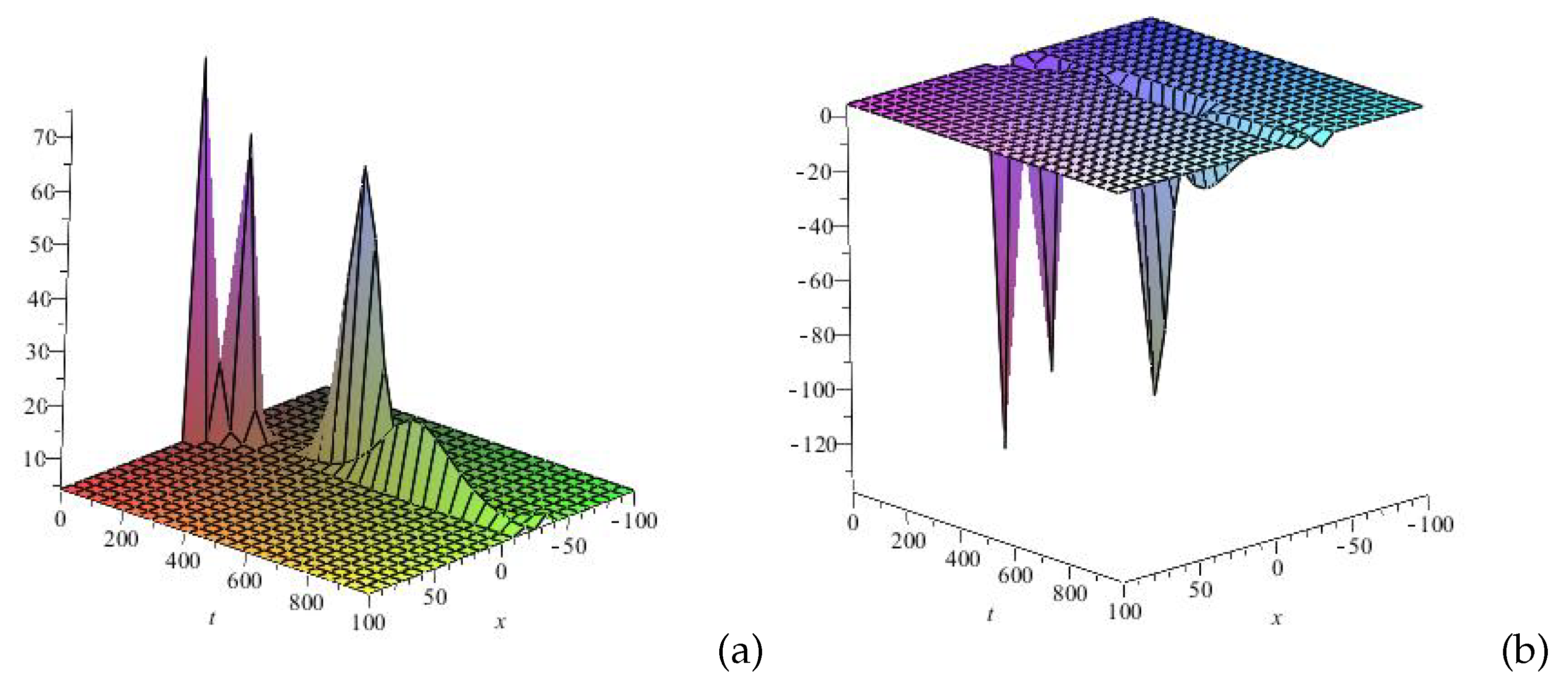
Figure 2.
Numerical simulation of the solution (38): (a) u(x,t) and (b) v(x,t) at .
Figure 2.
Numerical simulation of the solution (38): (a) u(x,t) and (b) v(x,t) at .
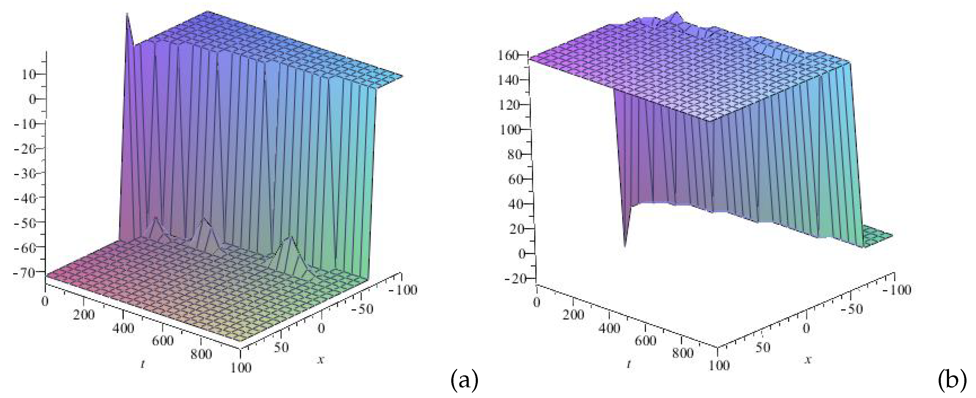
Figure 3.
Numerical simulation of the solution (41): (a) u(x,t) and (b) v(x,t) at .
Figure 3.
Numerical simulation of the solution (41): (a) u(x,t) and (b) v(x,t) at .
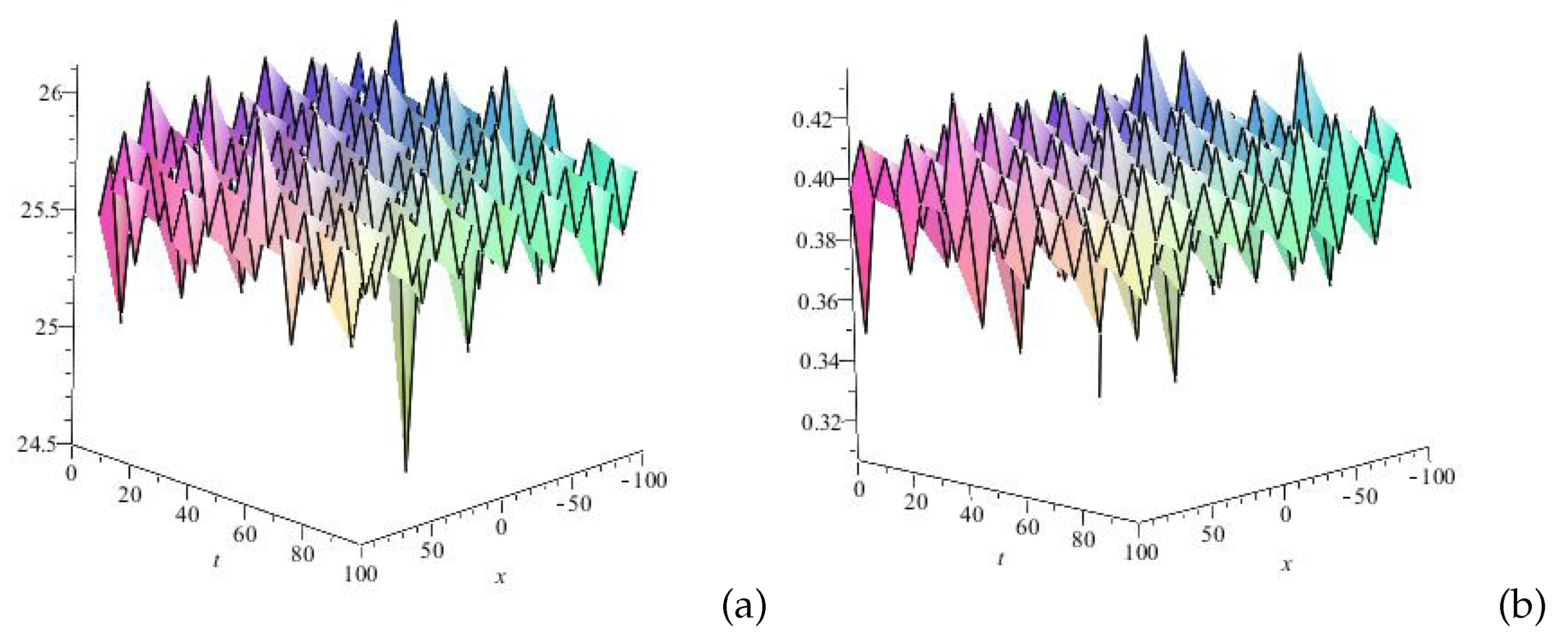
Figure 4.
Numerical simulation of the solution (46): (a) u(x,t) and (b) v(x,t) at .
Figure 4.
Numerical simulation of the solution (46): (a) u(x,t) and (b) v(x,t) at .
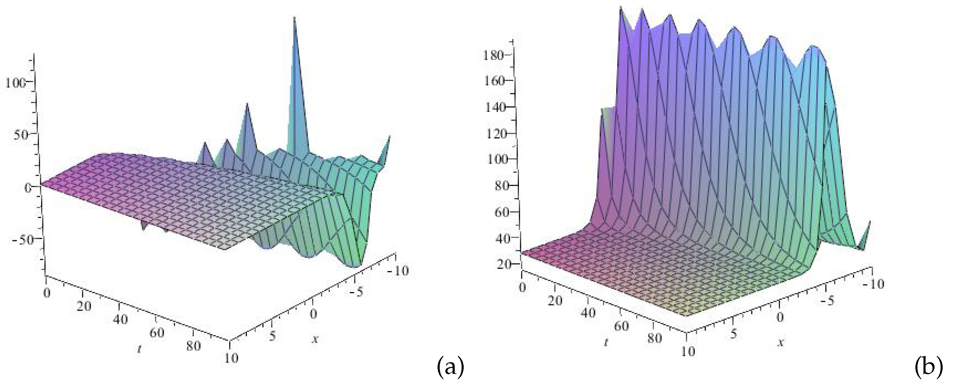
Figure 5.
Numerical simulation of the solution (50): (a) u(x,t) and (b) v(x,t) at .
Figure 5.
Numerical simulation of the solution (50): (a) u(x,t) and (b) v(x,t) at .
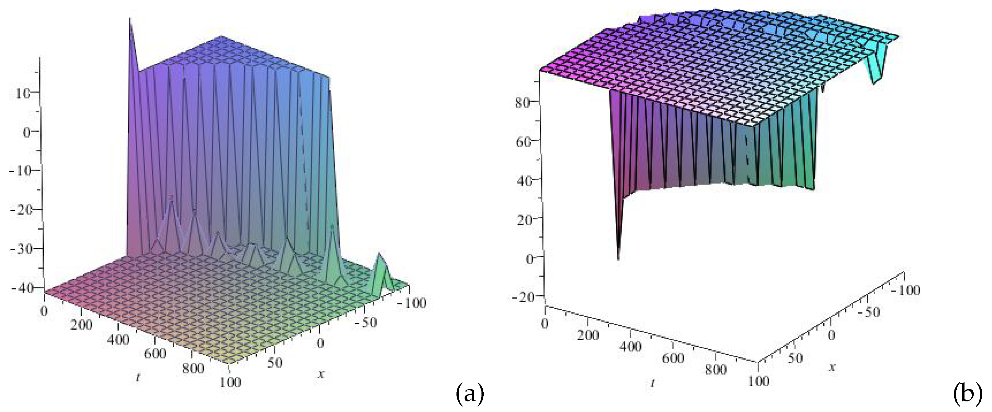
Figure 6.
Numerical simulation of the solution (55): (a) u(x,t) and (b) v(x,t) at .
Figure 6.
Numerical simulation of the solution (55): (a) u(x,t) and (b) v(x,t) at .
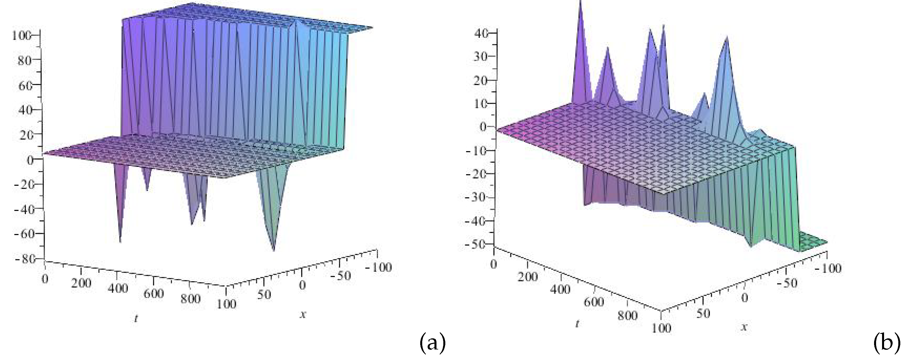
Figure 7.
Numerical simulation of the solution (59): (a) u(x,t) and (b) v(x,t) at .
Figure 7.
Numerical simulation of the solution (59): (a) u(x,t) and (b) v(x,t) at .
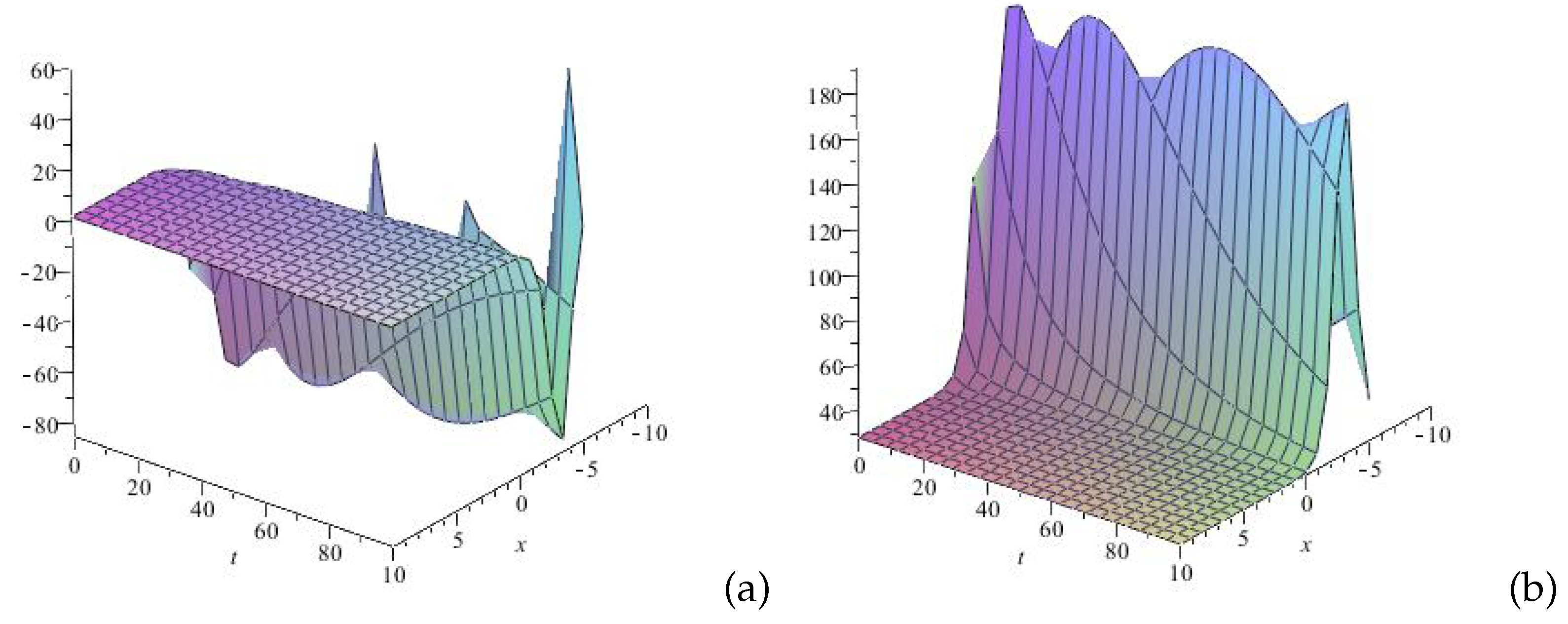
Figure 8.
Numerical simulation of the solution (75): (a) u(x,t) and (b) v(x,t) at .
Figure 8.
Numerical simulation of the solution (75): (a) u(x,t) and (b) v(x,t) at .
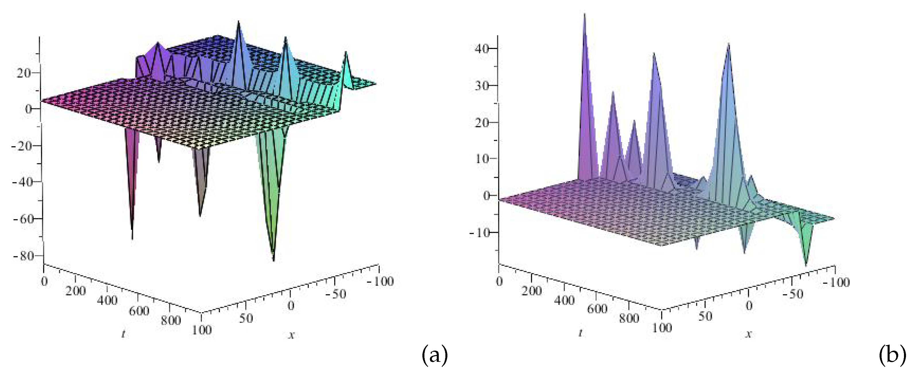
Figure 9.
Numerical simulation of the solution (83): (a) u(x,t) and (b) v(x,t) at .
Figure 9.
Numerical simulation of the solution (83): (a) u(x,t) and (b) v(x,t) at .
Disclaimer/Publisher’s Note: The statements, opinions and data contained in all publications are solely those of the individual author(s) and contributor(s) and not of MDPI and/or the editor(s). MDPI and/or the editor(s) disclaim responsibility for any injury to people or property resulting from any ideas, methods, instructions or products referred to in the content. |
© 2025 by the authors. Licensee MDPI, Basel, Switzerland. This article is an open access article distributed under the terms and conditions of the Creative Commons Attribution (CC BY) license (http://creativecommons.org/licenses/by/4.0/).
Copyright: This open access article is published under a Creative Commons CC BY 4.0 license, which permit the free download, distribution, and reuse, provided that the author and preprint are cited in any reuse.


