
Submitted:
23 September 2025
Posted:
25 September 2025
You are already at the latest version
Abstract
Due to the fact that an earthquake cannot be predicted, the simulation of earthquakes using earthquake simulators is of great importance. An earthquake simulator is a device that reproduces the seismic waves that all generated by an earthquake. The aim of this work is present the design and prototyping earthquake simulator that simulates a real long-period ground motion earthquake with vertical displacement, according to the earthquake seismogram. A prototype of an earthquake simulator for simulating a real long-period ground motion during an earthquake with a vertical displacement, according to a given earthquake seismogram, was designed. A control interface of the prototype earthquake simulator is designed, to handle reproducing a given earthquake seismogram. The mobile platform of the earthquake simulator prototype performs translational motions in the direction of the X and Y axes due to the use of a cable driven parallel robot, and the vertical translational motion of the platform along the Z axis is performed by linear screw drives. Experimental tests of the earthquake simulator prototype were carried out, which confirmed the feasibility of reproducing long-period ground motion during an earthquake.
Keywords:
earthquake simulators
; cable driven parallel robot
; design
; testing
1. Introduction
Earthquakes occur unexpectedly and produce catastrophic destruction. After 10-20 seconds of ground vibrations, tremors intensify, which leads to the destruction of buildings and structures. Due to the increase in the construction of tall buildings and industrial facilities, scientists and engineers pay great attention to the research of seismic waves that cause long-period ground motion [1]. Seismic waves of this type occur during very strong earthquakes and contain periodic motions within one to ten seconds. These waves propagate over long distances over the earth’s surface and excite low-frequency structural vibrations in multi-story buildings, which cause serious damage to people or objects inside the building.
Due to the fact that an earthquake cannot be predicted, the simulation of earthquakes using earthquake simulators is of great importance. An earthquake simulator is a device that reproduces the seismic waves that all generated by an earthquake. It is used for experimental researches on models of buildings and their foundations for seismic resistance, and even for seismic training of people. Earthquake simulators can reproduce real seismic waves from past earthquakes. Training on earthquake simulators helps to develop an effective response in people to earthquakes.
The earthquake simulator is used to conduct seismic training for people, to teach them how to behave during a real earthquake by employees of the Ministry of Emergency Situations [2]. In the world, at least hundreds of millions of people are exposed to significant seismic risk of catastrophic damage. This problem is especially acute in Almaty, Republic of Kazakhstan, where the last earthquake in the spring of 2024 caused panic among people and showed a complete lack of preparedness for how to feel and behave when an earthquake occurs [3]. Earthquakes pose a danger and risk to all people, and everyone needs to know the appropriate knowledge and protective measures.
The main requirement for an earthquake simulator is to reproduce a given seismogram of an earthquake (see Figure 1) along three Cartesian axes. For example, Figure 1 shows a seismogram of the foundation of a house during the long-period ground motion earthquake of 1964 in the city of Niigata (Japan) [1].
Various types of earthquake simulators have been developed to reproduce seismic waves as for example those designs in [4,5,6,7,8,9,10,11,12,13,14]. In Japan, a large earthquake simulator E-Defense [15] was built to reproduce various seismic waves with high accuracy. The E-Defense Earthquake Simulator has a 20m x 15m moving platform with 14 hydraulic drives and therefore cannot be transported. The work [16] presents a portable earthquake simulator Jishin-The-Vuton 3D, which implements up and down motion to simulate three-dimensional ground motion during an earthquake. The disadvantage of the Jishin-The-Vuton 3D simulator is the tendency to tip over due to the small contact area of the drive system with the person sitting on it.
An earthquake simulator [17] with a vibrating platform, which is mounted on a frame, has been developed. The platform is driven reciprocating motion by a hydraulic drive through a system of linkages. The disadvantage of this earthquake simulator is the complexity of the design and control due to the presence of hydraulic drives, the impossibility of reproducing large accelerations, low transportability, and unsuitability for seismic training of people. It does not have the ability to simulate a long-period ground motion earthquake.
An earthquake simulator based on the spatial parallel mechanism 4-RPS (Range Positioning System) [18] was developed and installed on a truck. The earthquake simulator is mobile, simple in structure, flexible and accurate in operation, and can be widely used for the scientific promotion of earthquake research in schools and communities. The disadvantage of this earthquake simulator is the impossibility of modeling a long-period ground motion earthquake.
The paper [19] presents a study of the possibility of using CaPaMan (Cassino Parallel Manipulator) as an earthquake simulator. The results of numerical tests confirm the possibility of simulating any type of seismic motion using CaPaMan. The paper [20] presents an earthquake simulator based on CaPaMan for reproducing three-dimensional seismic motions with easy-to-use and reliable functions. The results of experimental tests simulating a three-dimensional earthquake are shown. The paper [21] presents an experimental characteristic of the influence of CaPaMan capable of simulating seismic vibrations in three-dimensional space quite well. The disadvantage of the earthquake simulator based on CaPaMan is the impossibility of simulating a long-period earthquake.
In [22], an earthquake simulator based on a planar cable parallel mechanism was built. Due to the use of cables, a large working space is achieved, and due to the low inertia of the moving platform, the simulator is able to simulate high accelerations. In addition, it has easy assembly and disassembly and high transportability. The platform of the earthquake simulator performs a plane-parallel motion in the direction of the X and Y axes due to the tension of the cables by servomotors, and thereby simulating the longitudinal and transverse earthquake waves.
The disadvantage of this earthquake simulator is the complexity and high cost of the design due to the presence of air bearings, the unstable operation of which causes problems with platform stability. In addition, the earthquake simulator reproduces seismic waves only in the direction of the X and Y axis, while to reproduce the real seismogram of the long-period ground motion earthquake shown in Figure 1, the motion of the platform in the direction of the Z axis is necessary.
To eliminate the above disadvantages of earthquake simulators, in this paper, an earthquake simulator is designed to reproduce three-dimensional long-period ground motion during an earthquake.
The aim of this work is present the design and prototyping earthquake simulator that simulates a real long-period ground motion earthquake with vertical displacement, according to the earthquake seismogram. The earthquake simulator performs translational cartesian motions. The mobile platform of the earthquake simulator moves with translational motions in the direction of the X and Y axes due to the use of cable driven parallel robot (CDPR), and the vertical translational motion of the platform along the Z axis will be performed by linear screw drives.
2. Materials and Methods
2.1. Design of an Earthquake Simulator
Figure 2 shows a structural scheme of an earthquake simulator for reproducing three-dimensional long-period ground motion during an earthquake. To reproduce the translational motion of the mobile platform along the X and Y axes, we use a CDPR with 4 cables that are controlled by 4 servomotors. The mobile platform makes planar motions on the floor (fixed base) using nine ball caster wheels. We install a vertical moving platform on the mobile platform to reproduce the vertical translational motion along the Z axis. The vertical moving platform moves along the Z axis on four linear screw guides with the help of four stepper motors. For testing, the object or person is placed on a vertical moving platform.
To reproduce a given seismogram, the earthquake simulator works as follows. The computer, using a specially designed program, issues signals for control to the servomotor controllers. Servo motors begin to stretch the cables by winding and unwinding winches on drums, motion the mobile platform horizontally along the X, Y axes, and thereby simulating the longitudinal and transverse waves of an earthquake. To carry out the vertical motion of the platform, four stepper motors are switched on synchronously.
The advantages of this constructive scheme of the earthquake simulator (see Figure 2) consist in the simplicity of design, its assembly and disassembly and high transportability, and most importantly, in the possibility of realizing the vertical motion of the platform.
2.2. Kinematics of a CDPR
Let us consider the kinematics of a 4-cables CDPR, by which the mobile platform performs translational motions in the direction of the X and Y axes. The kinematic scheme of a CDPR with four cables is shown in Figure 3. The fixed base is determined by the plane identified by four cable drive points . The global coordinate system {XYZ} is set to the center of the base. The local coordinate system {xyz} is located in the geometric center P of a rectangular platform with vertices at the connection points of the cables .
In Figure 3, is the position vector of point attached to the fixed frame relative to the main coordinate system {XYZ}, is the position vector of the point , is the length vector of the cables relative to the main coordinate system XYZ. The dimensions of the fixed rectangular frame CDPR are given by width and length. Dimensions of the square mobile platform CDPR: dp - side length. In the kinematic scheme of the CDPR, it is assumed that the cables are straight and stretched. In addition, it is assumed that the vectors and do not depend on the position of the mobile platform, i.e., the influence of possible guide pulleys or fasteners on the platform is not taken into account.
Applying the method of closed vector loops (see Figure 3) we obtain the following system of equations
where the vector is the Cartesian position of the P center of the mobile platform, relative to the global coordinate system {XYZ}. Here, the coordinate is constant and equal to the height of the cables fastening relative to the base because the cables act on a plane.
Equations (1) can be written as
The unit vector in Equation (1) along the cable can be expressed as
The unit vector is directed from the mobile platform to the fixed base, which means that the positive forces are directed in the direction that shortens the cables and thereby reduces the value of the generalized coordinate associated with it. The coordinates of the vector , relative to the main XYZ coordinate system, are given in Table 1 as referring to mechanical design of the scheme in Figure 2.
The coordinates of the vector , relative to the local coordinate system xyz, are given in Table 2
To solve the direct task of the kinematics of a CDPR, from Equation (1) we obtain 4 nonlinear equations of direct kinematics, which form a system with redundant constraints [23].
Here we consider cables as linear springs. In general, we cannot expect the above equations to be solved exactly, but we can minimize the error, which can be interpreted as minimizing the potential energy in the pretensioned cables. Let be the potential energy of the system
where is the stiffness of the i-th cable. We assume that all cables have the same stiffness . Then the minimum potential energy U of the system does not depend on the specific stiffness value and the direct kinematics function can be determined from the optimization problem [23]
where the vector is the given cable lengths. The function gives the values providing the minimum of Equation (6). As a result of solving problem (6), we obtain the coordinates of the platform, with given lengths of the cables.
2.3. Statics of a CDPR
For the balance of forces and moments of the movable platform of a CDPR that performs only translational motion, it is necessary to take into account all the forces acting on the mobile platform. Figure 4 is a scheme for considering all these actions.
From Figure 4 the equilibrium condition for the mobile platform can be expressed
The force of the i -th cable applied to the movable platform at point can be expressed as . Here is an external force. – the reaction from the force of gravity of a moving platform of mass Can write Equation (7) in matrix form
where is the CDPR structural matrix, is the cable force vector,
Determining the cable force can be considered as a solution to the matrix problem in Equation (8), which consists in finding the vector T in a given range and satisfying Equation (8). For the normal operation of the CDPR, the following conditional must be met
where and _max are the minimum and maximum cable forces, respectively.
For CDPR with redundant constraints, it is difficult to directly determine the forces of cables, the optimal task of minimizing the Euclidean norm of forces in cables is formulated [24].
The optimization task is in the form
under the constraints defined by Equations (8) and (9).
The optimization task Equation (10) with constraints defined by Equations (8) and (9) is a quadratic programming task that can be solved using iterative algorithms for solving quadratic programs in general MATLAB optimization packages. The external force in the earthquake simulator is the friction force between the ball caster wheels and the fixed base. The Equation (10) give the solution for the tension force in the cables for a static equilibrium.
2.4. Dynamic Model of a CDPR
The dynamic equations of the mobile platform of a CDPR can be derived, considering the scheme in Figure 5.
From Figure 5 as the force equilibrium can be expected
where, is the mass of the mobile platform concentrated in the center of mass, is the velosity of the center of mass of the mobile platform. Substitute in Equation (11) the expression , then in matrix form the dynamic equation looks like
where is the CDPR structural matrix, is the cables force vector, – dynamic force acting on the platform.
Let us consider the dynamics of the CDPR drive, which consists of a servomotor shaft with lumped parameters and a winch drum for winding a cable. The dynamic model for the servomotor shaft and the cable winding drum is shown in Figure 6.
In Figure 6: is the angle of rotation of the i -th drive motor, is the radii of the i-th winch drums, is the moment of inertia of the i-th servomotor and the winch drum is the torque of the i-th servomotor, is the dissipation coefficient i -th drive (i=1,..,4).
The dynamic equation for the servomotor shaft and the cable winch drum is
where
,
,
,
,
,
,
Assuming that the torque of the CDPR drive servomotors keeps the cables in tension, from Equation (13) we determine the tension of the cables as a function of the torques of the drive motors:
The general model of the dynamics of the CDPR system is obtained by combining the equations of motion of the platform and the drive. To obtain an equation relating the i-th angles of rotation of the drive motor with the position of the end effector , we assume that all are equal to zero when the geometric center of the platform is located at the origin of the frame base .
The change in the length of the i-th cable is equal to , where is the length of the cable obtained from the solution of the inverse kinematics problem, and is the initial length of the i-th cable.
For convenience, let’s rename the position vector of the final effector to , i.e., .
The successive time derivatives of Equation (16) have the form:
Substituting Equations (17) and (18) into Equation (14) gives:
Substitute Equation (19) into Equation (12), then we get
Let us write the Equation (20) of motion of the CDPR in the standard Cartesian form [25].
Where is the equivalent inertia matrix and non-linear terms:
(
Here is the identity matrix.
They, the formulation with Equations (14)-(23) can be used to solve the servomotor torque that generate the proper cable tension for the platform motion.
2.5. Linear Drive of Vertical Moving Platform
For the earthquake simulator to reproduce the given earthquake seismogram (Figure 1) along the Z axis, it is necessary to ensure the translational motion of the vertical moving platform. To ensure the motion of the vertical moving platform, four linear drives with ball screw transmission are used, which are installed at the tops of the rectangular platform. Figure 7 shows a ball screw linear actuator that is designed to lift a vertical moving platform. The drive consists of a stepper motor connected through a coupling with a lead screw with a nut mounted on a linear guide, a slide is fixed on the nut, which is connected to a vertical moving platform.
The dependence of the slide stroke on the angle of rotation of the screw is determined by the formula
where is the pitch of the screw.
The linear velocity of the slider is determined by the formula
where .
The gear ratio of the screw gear is . The torque of the stepper motor is determined by the formula
The value of the slide acceleration is taken from the earthquake seismogram acceleration graph, is ¼ of the mass of the vertical moving platform with a load.
2.6. Control System of a CDPR
The control system of a CDPR can be developed on the basis of the equation of motion of the CDPR in the standard Cartesian form Equation (23). The input parameters of the CDPR are the torque vector of the actuator . Each component of the vector must be positive or at least equal to zero (usually a small positive value).
Let’s introduce a virtual generalized input Cartesian force [25]
Since the structure matrix has a dimension of 3x4, because is 1x4 this virtual generalized input Cartesian force has a translational Cartesian space dimension of 3. Components of are not limited to positive values.
If you develop a control for the input virtual Cartesian force , you can always find the real control input torque with all positive components that satisfies Equation (27) if the position of the CDPR is within the static workspace. Consider a dynamics equation:
We use a Cartesian PD controller to monitor the positioning error
where is the given Cartesian position. The calculated torque control law for the input virtual Cartesian force can be expressed as
are 2x2 diagonal matrix gains. The inertial terms consist of a common Cartesian matrix of inertia depending on the position of and the Cartesian acceleration components ; non-linear terms are .
In Equation (30), the influence of the terms of the nonlinear dynamics is excluded and the inertial terms are taken into account using the calculated torque method [26]. Equation (30) uses the desired Cartesian values of . Using the actual values from the feedback from the actuator encoder sensors and the forward kinematics solution causes problems with sensor noise and double digital differentiation errors.
The control scheme of the CDPR is shown in Figure 8, and consists of: a PD controller, a block for determining the virtual generalized input Cartesian force , a block for calculating the real torque of the drive (Virtual to Real Calculation) with dynamic estimation of the minimum torque (Minimum Torque Estimation ) to ensure constant maintenance of the cable tension, despite the dynamics of the CDPR.
The position of the X is determined using the feedback of the encoder, which gives the rotation angles of the i -th drive motor to determine the lengths of the cables . Further, by solving the direct kinematics of the CDPR (6), we determine the Cartesian position . This feedback scheme will work well only if sufficient tension is constantly maintained on all cables [25].
For control, we need to calculate the real torques of the actuator τ, taking into account the virtual forces . The solution of the insufficiently bounded system is similar to the solution of the optimization task Equation (10).
For normal operation of the CDPR, the cable tension vectors must always be positive during its operation.
The calculation of the minimum torque for each drive to maintain the tension of the cables is determined from Equation (31)
Equation (32) makes it possible to dynamically estimate the minimum tension of each CDPR cable and prevents sagging during its motion when the condition is met.
3. Experimental Test Results
3.1. Earthquake Simulator Prototype
To assemble the earthquake simulator prototype, a configuration of its system was developed, shown in Figure 9.
The prototype is assembled as in Figure 10 according to design schemes in Figure 9. The prototype of the earthquake simulator consists of a CDPR with four Dyneema, LIROS D-Pro 01505-0200 cables with a diameter of 3 mm. Each cable is set in motion by a drive. The drive consists of an AC servomotor with a power of 600 W, which is connected to a winch through a planetary reducer with a gear ratio of 1: 10 and a gear transmission with a gear ratio of 1: 3. The drives are installed on the floor, in the corners of a square measuring 2.7 x 2.7 m. The CDPR cables are attached, through S Type Load Cells DYLY-101 force sensors [27], to a mobile platform measuring 0.8 x 0.8 x 0.8 m. The motion of the vertical movable platform is performed by four drives, which are installed at the vertices of the platform. The drive consists of a hybrid stepper motor (Hybrid stepper motor) Nema34 - 86HB250-156 B and a ball screw transmission. The mass of the earthquake simulator prototype is 30 kg.
For operation of the earthquake simulator prototype, it is necessary to maintain the desired minimum tension of the cables throughout its entire operation. For this purpose, the control system takes into account data from the S Type Load Cells DYLY-101 force sensors [27]. The signal on the level of cable tension from these sensors is sent to the Mach 3 controller, which is connected to the computer via the USB port. The value of the minimum tension in the cables of the spatial CDPR will be maintained, taking into account the data received from the force sensors, during its operation. The force sensors are connected to the ZET 058 [27] measuring strain gauge system, which, together with the ZETLAB TENZO software [27], allows collecting information from the force sensors in real time on four channels simultaneously.
Figure 11 shows the program interface for controlling the earthquake simulator prototype.
Using the control interface of the earthquake simulator prototype, we can reproduce a given earthquake seismogram. In addition, there is the possibility of manual control of the translational motion of the earthquake simulator prototype: forward-backward, left-right.
3.2. Experiment of Motion Simulation of Earthquake
Test have been carried out at the laboratory of Joldasbekov Institute of Mechanics and Engineering to prove the feasibility of proposed earthquake simulator and to investigate on potential new application.
3.2.1. Testing Basic Motion Components
Test are carried to check the planar motion replicas along plane cartesian axes. The first test was along X axis with seismic trajectory of the simulator platform in the form
Equation (33) describes the motion of the platform in the direction of the X-axis, with a maximum amplitude within ± 0.2 m. The equation of motion is given as a sine wave with a frequency of 0.5 Hz, the amplitude of which is modulated by an envelope with a frequency of 0.05 Hz.
Measurements of the platform trajectory in the direction of the X-axis motion were carried out using a BRT38-ROM1024D99-RT1 rope displacement sensor [28] as in Figure 12. The BRT50-V5M-RT1 rope displacement sensor is designed for linear measurements of movements in links of mechanisms, machines and robots. For linear positioning, the sensor has feedback on the displacement value. The linear accuracy is ± 0.1%, and the repeat accuracy is ± 0.01%. The calculated travel length is determined by the sensor using the formula, [28]
L = (X2-X1) * C / P
where P is the sensor resolution, C is the diameter of the inner wheel, X1 and X2 are the position values before and after the pulling cable, determined by the sensor encoder.
Figure 13 shows the desired, measured and error trajectories of the platform motion of a test using the rope displacement sensor in Figure 12.
Acquired the acceleration of the platform in the direction of the X-axis, measurements were made using the WHEELTEC N200 inertial measurement unit [29]. The WHEELTEC N200 is an inertial measurement unit (IMU) with 9 DOF in a single package. It contains a 3-axis accelerometer, 3-axis gyroscope, 3-axis magnetometer. Figure 14a shows the desired and measured accelerations of the platform in the X-direction. Figure 14b shows the desired and filtered measured accelerations of the platform in the X-direction.
The characteristics of the desired acceleration in the X-direction are: total time 10 sec, maximum amplitude within ±2 m/s2, frequency 0.5 Hz (period 2 sec). The characteristics of the measured filtered acceleration (see Figure 14b) in the X-direction are approximately the same: maximum amplitude error ±0.4 m/s2, in frequency there are small deviations at the beginning and at the end. Therefore, the earthquake simulator can provide accelerations in the X-direction along the desired trajectory given by Equation (30) of the platform movement.
The measurements of cable tensions of the CDPR platform were carried out using force sensors connected to the ZET 058 [27] measuring strain gauge system. Figure 15 shows the cable tensions of the platform CDPR during movement in the direction of the X-axis, obtained from strain gauge. As can be seen from Figure 15, the cable tensions have positive values and have oscillations that coincide in frequency with the acceleration. The cable tensions have significant oscillations from the sinusoidal shape, which causes errors in ensuring the acceleration of the platform in the X-axis direction. The cable tension graph is necessary for assessing the operation of the earthquake simulator. To eliminate cable tension oscillations, it is necessary to increase the initial cable tension as much as possible [22].
Let us consider the additional motion of the simulator platform in the direction of the Y axis to get a planar motion that is desired by
Equation (35) describe the trajectory of the platform motion in the direction of the X axis, with a maximum amplitude within ± 0.2 m, and in the direction of the Y axis with a maximum amplitude within ± 0.05 m. The equations of motion along the X and Y axes are desired as a sinusoidal wave with a frequency of 0.5 Hz, the amplitude of which is modulated by an envelope with a frequency of 0.05 Hz. According to equations (35), the platform moves diagonally. Measurements of the platform trajectory in the direction of the X-axis motion and Y-axis motion were carried out using a BRT38-ROM1024D99-RT1 rope displacement sensor [28]. Figure 16 shows the desired and measured trajectories of the platform motion.
The measurements of cable tensions of the CDPR platform were carried out using force sensors connected to the ZET 058 [27] measuring strain gauge system. Figure 17 shows the tension of the CDPR cables when the platform moves along the trajectory described by Equation (35).
The trajectory tracking error (see Figure 16) occurs due to a decrease in cable tension (see Figure 17), as a result of a sharp change in platform acceleration. To eliminate cable slackening, work [22] suggests increasing the initial cable tension as much as possible.
A vertical motion of the simulator platform in the direction of the Z axis was tested using a motion given by
Equation (36) describes the trajectory of the platform motion in the direction of the Z axis with a maximum amplitude within ± 0.05 m. The equation of motion along the Z axis is given as a sinusoidal wave with a frequency of 0.5 Hz, the amplitude of which is modulated by an envelope with a frequency of 0.05 Hz. Measurements of the platform trajectory in the direction of motion of the Z axis were carried out using a BRT38-ROM1024D99-RT1 rope displacement sensor. Measurements of the platform acceleration in the direction of motion of the Z axis were carried out using a WHEELTEC N200 inertial measurement unit.
Figure 18 shows the desired, measured and error trajectories of the platform motion in the direction of motion along the Z axis.
The platform acceleration measurements in the direction of motion of the Z axis were carried out using the WHEELTEC N200 inertial measurement unit. Figure 19 shows the desired and measured accelerations of the platform in the Z-axis direction.
The measured acceleration characteristics in the Z-axis direction are approximately the same: the maximum amplitude error is ±0.145 m/s2, there are deviations in frequency. It follows that in order to ensure acceleration of the platform movement in the Z-axis direction along a trajectory given by Equation (36), it is necessary to further improve the mechanism for the platform motion in the Z-axis direction.
3.2.2. Testing a Replica of a Real Earthquake
Let’s conduct an experiment to reproduce a real earthquake seismogram with a prototype earthquake simulator. Figure 20 shows a real seismogram of the San Fernando earthquake near Pacoima Dam, California, in 1971 [30].
We will digitize the graphs of the real seismogram using the PlotDigitizer program [31], which allows extracting numerical data from images. We will use the digitized movements of the real seismogram to determine the lengths of the CDPR cables using Equation (2). Figure 21 shows the graphs of the CDPR cable lengths. By changing the cable lengths, the movement of the mobile platform of the earthquake simulator is carried out according to the desired real seismogram shown in Figure 20.
Figure 22 shows the desired, measured and error displacements of the platform according to the real seismogram of the San Fernando earthquake.
Figure 23 shows the desired, measured accelerations of the platform according to the real seismogram of the San Fernando earthquake. The characteristics of the desired acceleration are: total time 12 sec, maximum amplitude within ±1.055 m/s2. The characteristics of the measured acceleration of the platform are approximately the same: maximum amplitude error ±0.3 m/s2. Thus, the earthquake simulator can provide platform accelerations consistent with the real San Fernando seismogram (see Figure 20).
The conducted test showed good capabilities of the earthquake simulator to reproducing a real earthquake seismogram using a prototype earthquake simulator. The earthquake simulator implements motions that are practically indistinguishable from real tremors and seismic vibrations, thereby causing a person to experience sensations close to those experienced in real earthquakes. It should be noted that during the tests, a person distinguished the difference in sensations when the earthquake simulator reproduced a sinusoidal earthquake and a real earthquake. Video materials depicting experimental tests are presented in the [32].
4. Conclusions
This paper presents a prototype of earthquake simulator for reproducing three-dimensional, long-period ground motion during an earthquake, simulating real earthquake seismograms. The mobile platform of the prototype earthquake simulator performs planar motion in the direction of the X and Y axes due to the tension of the CDPR cables, and the vertical translational motion of the platform along the Z axis is performed by linear screw drives.
A control interface of the prototype earthquake simulator is designed, to handle reproducing a given earthquake seismogram. In addition, there is the possibility of manual control of the translational motion of the prototype earthquake simulator: forward-backward, left-right.
Experimental tests of the earthquake simulator prototype were conducted successfully with trajectories of the mobile platform motion in the direction of the X, Y axis and the motion of the vertical platform in the form of a sinusoidal wave with a frequency of 0.5 Hz, the amplitude of which is modulated by an envelope with a frequency of 0.05 Hz. The following maximum amplitudes were desired along the X axis within ± 0.2 m, along the Y axis within ± 0.05 m, along the Z axis within ± 0.05 m. The results of the experimental tests have shown the ability of the developed prototype earthquake simulator to well reproduce a seismogram of a three-dimensional, long-period ground motion during an earthquake.
Future work is planned to increase the accuracy of reproducing a real occurred seismogram of a three-dimensional, long-period ground motion during an earthquake. Improve the mechanism for moving the platform in the vertical direction to more accurately and to ensure acceleration of the platform’s movement along a given trajectory. Then application of the simulator is expected in conducting experimental researches on the stability of building models and their foundations during a three-dimensional, long-period earthquake together with investigation on human reaction to earthquake motion.
Author Contributions
Conceptualization, A.J., M.C.; methodology, A.J., M.C. and A.T.; software, A.J., A.K.; validation, A.J., M.C.; formal analysis, A.J., M.C.; investigation, A.J., M.C.; resources, A.A.; data curation, A.K.; writing—original draft preparation, A.J., M.C; writing—review and editing, A.J., M.C; visualization, A.A., A.K.; project administration, A.J.
Funding
This research was funded by the Science Committee of the Ministry of Science and Higher Education of the Republic of Kazakhstan Grant No. AP26195455.
Data Availability Statement
No new data were created or analyzed in this study.
Conflicts of Interest
The authors declare no conflicts of interest.
References
- Koketsu, H.; Miyake, H. A Seismologies Overview of Long-Period Ground Motion. Journal of Seismology 2008, 12, 133-143. [CrossRef]
- The Ministry of Emergency Situations of the Republic of Kazakhstan. Available online: https://www.gov.kz/memleket/entities/emer?lang=en (accessed on 16 September 2025).
- Eurasianet. Available online: https://eurasianet.org/kazakhstan-strong-earthquake-plunges-almaty-into-panic (16 September 2025).
- Advanced Earthquake Engineering Laboratory. Available online: https://www.shimz.co.jp/en/company/about/sit/facility/facility04/ (16 September 2025).
- Earthquake Simulator Laboratory. Available online: https://peer.berkeley.edu/earthquake-simulator-laboratory (16 September 2025).
- Earthquake Simulator. Available online: https://motionsystems.eu/portfolio/earthquake-simulator/ (16 September 2025).
- Earthquake Simulator ST115. Available online: https://bedoeg.com/product/st115/ (16 September 2025).
- Earthquake Simulator SYSMO. Available online: https://3r-labo.com/en/produit/sysmo-earthquake-simulator/ (16 September 2025).
- Seismic Simulators (Shake Tables). Available online: https://www.mts.com/en/products/civil-engineering/seismic-simulators (16 September 2025).
- Seismic Simulators (Shake Tables) Available online: https://simton.co.th/product/seismic-simulators-shake-tables/ (16 September 2025).
- Desktop servo electro mechanical shake table. Available online: https://tdg.com.tr/en/products/desktop-shake-tables/tdg-shaketable-uniaxial (16 September 2025).
- Earthquake simulator - Quake Cottage. Available online: https://tdg.com.tr/en/products/desktop-shake-tables/tdg-shaketable-uniaxial/ (16 September 2025).
- Earthquake Simulator. Available online: https://scanalyst.fourmilab.ch/t/an-earthquake-simulator/1928 (16 September 2025).
- Quanser Shake Table III XY. Available online: https://www.quanser.com/products/shake-table-iii-xy/ (16 September 2025).
- Ohtani, K.; Ogawa, N.; Takayama, T.; Shibata, H. Construction of E-DEFENSE (3-D lull-scale earthquake testing facility). In Proceedings of the Third tenth World Conference on Earthquake Engineering, 2001.
- Roh, S.; Taguchi, Y.; Nishida, Y.; Yamaguchi, R.; Fukuda, Y. Kuroda, S.; Minoru, Y.; Fukushima, E.F.; Hirose, S. Development of the Portable Ground Motion Simulator of an Earthquake, Member. In Proceedings of the IEEE // 2013 IEEE/RSJ International Conference on Intelligent Robots and Systems (IROS), Tokyo, Japan, November 3-7, 2013. [CrossRef]
- Ouellette, J.F.; Poeling, D.L. Earthquake Simulator. USA Patent US №4112776А, 12 Sept. 1978.
- Li, B.; Wang, L.; Liu, Y.; Zheng, S. Vehicular earthquake simulator based on 4-RPS (Range Positioning System) space parallel mechanism. Huaiyin Institute of Technology. China Patent CN №101819727A, 1 Sept. 2010.
- Carvalho, J.C.M.; Ceccarelli, M. Seismic motion simulation based on cassino parallel manipulator. Journal of the Brazilian Society of Mechanical Sciences 2002, 24, 213-219. [CrossRef]
- Ceccarelli, M.; Ottaviano, E.; Florea, C.; Itul T.P.; Pisla, A. An experimental characterization of earthquake effects on mechanism operation. In Proceedings of the 2008 IEEE International Conference on Automation, Quality and Testing, Robotics, Cluj-Napoca, Romania, 2008. [CrossRef]
- Selvi1, Ö.; Ceccarelli, M.; Aytar, E. Effects of earthquake motion on mechanism operation: an experimental approach. International Journal of Mechanics and Control, 2015, 16, 25.
- Matsuura, D.; Ishida, S.; Akramin, M.; Küçüktabak, E.; Sugahara, Y.; Takeda, Y.; Fukuwa, N; Yoshida, M. Conceptual Design of a Cable Driven Parallel Mechanism for Planar Earthquake Simulation. In Proceedings of the 21 CISM-IFToMM Symposium on Robot Design, Dynamics and Control, Italy, Udina, 20 June-23 June 2016. [CrossRef]
- Pott, A. Cable-Driven Parallel Robots. Theory and Application, Springer International Publishing AG, part of Springer Nature, 2018.
- Gosselin, C; Grenier, M. On the determination of the force distribution in over constrained cable-driven parallel mechanisms. Meccanica 2011, 46, 3–15. [CrossRef]
- Williams II, R.L; Gallina, P. Translational Planar Cable-Direct-Driven Robots. Journal of Intelligent and Robotic Systems 2003, 37, 69–96. [CrossRef]
- Lewis, F.L.; Abdallah, C.T.; Dawson, D.M. Control of Robot Manipulators, MacMillan, New York, 1993.
- ZETLAB Company. Available online: www.zetlab.com (16 September 2025).
- Rope displacement sensors BRT50-V5M-RT1. Available online: www.briterencoder.com (16 September 2025).
- WHEELTEC N200 ROS IMU module, https://wheeltec.net/product/html/?180.html (16 September 2025).
- Encyclopædia Britannica, Inc. Available online: https://www.britannica.com/science/earthquake-geology/Methods-of-reducing-earthquake-hazards#/media/1/176199/19829 (16 September 2025).
- PlotDigitizer. Available online: https://plotdigitizer.com/app (16 September 2025).
- Jomartov, A.; Kamal, A. Design of an Earthquake Simulator Based on a Cable Driven Parallel Robot. Mendeley Data 2025. V1, https://data.mendeley.com/*************** . will be attached soon.
Figure 1.
Seismograms of the 1964 Niigata earthquake observed at the basement of a damaged apartment house.
Figure 1.
Seismograms of the 1964 Niigata earthquake observed at the basement of a damaged apartment house.
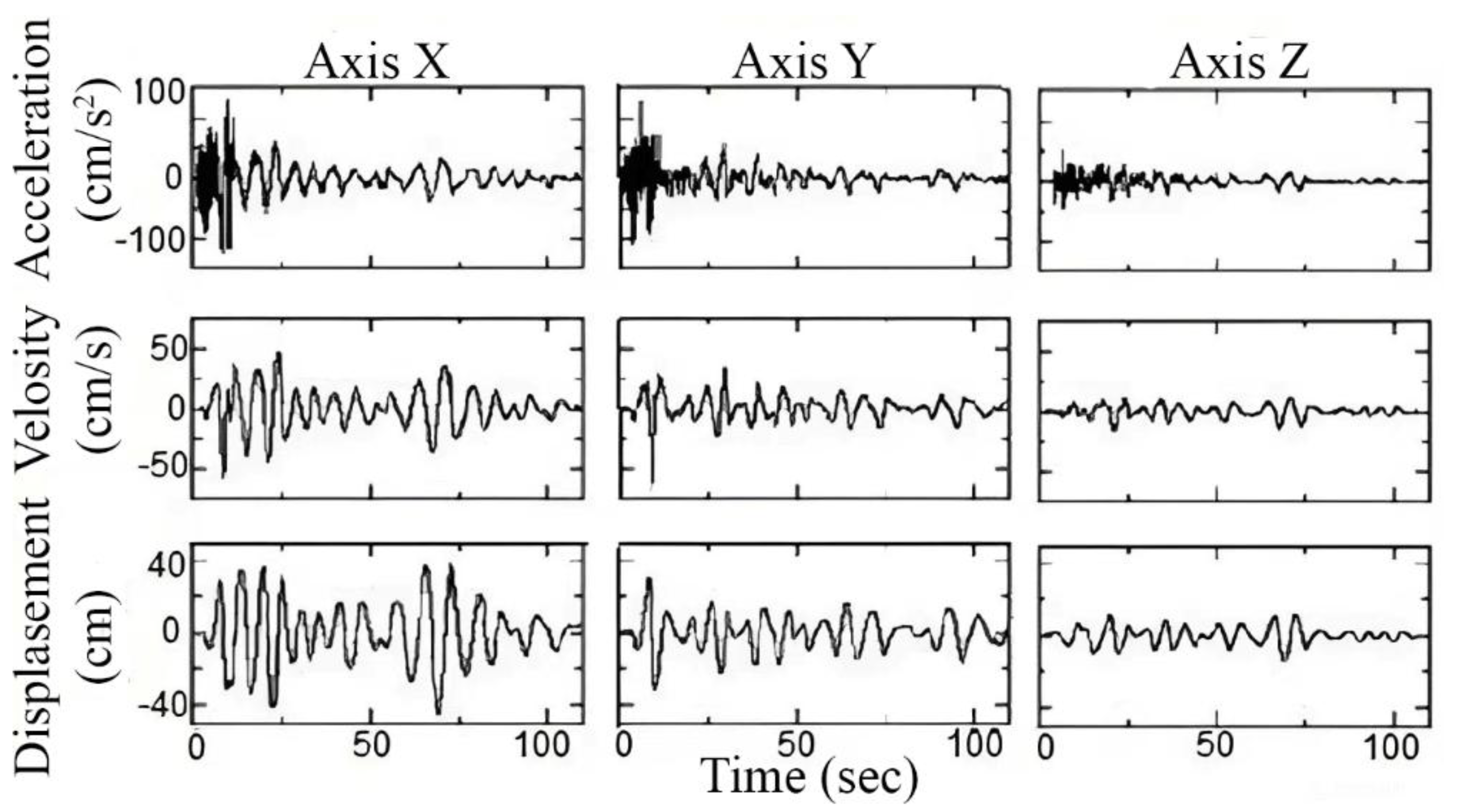
Figure 2.
Structural scheme of the proposed earthquake simulator.
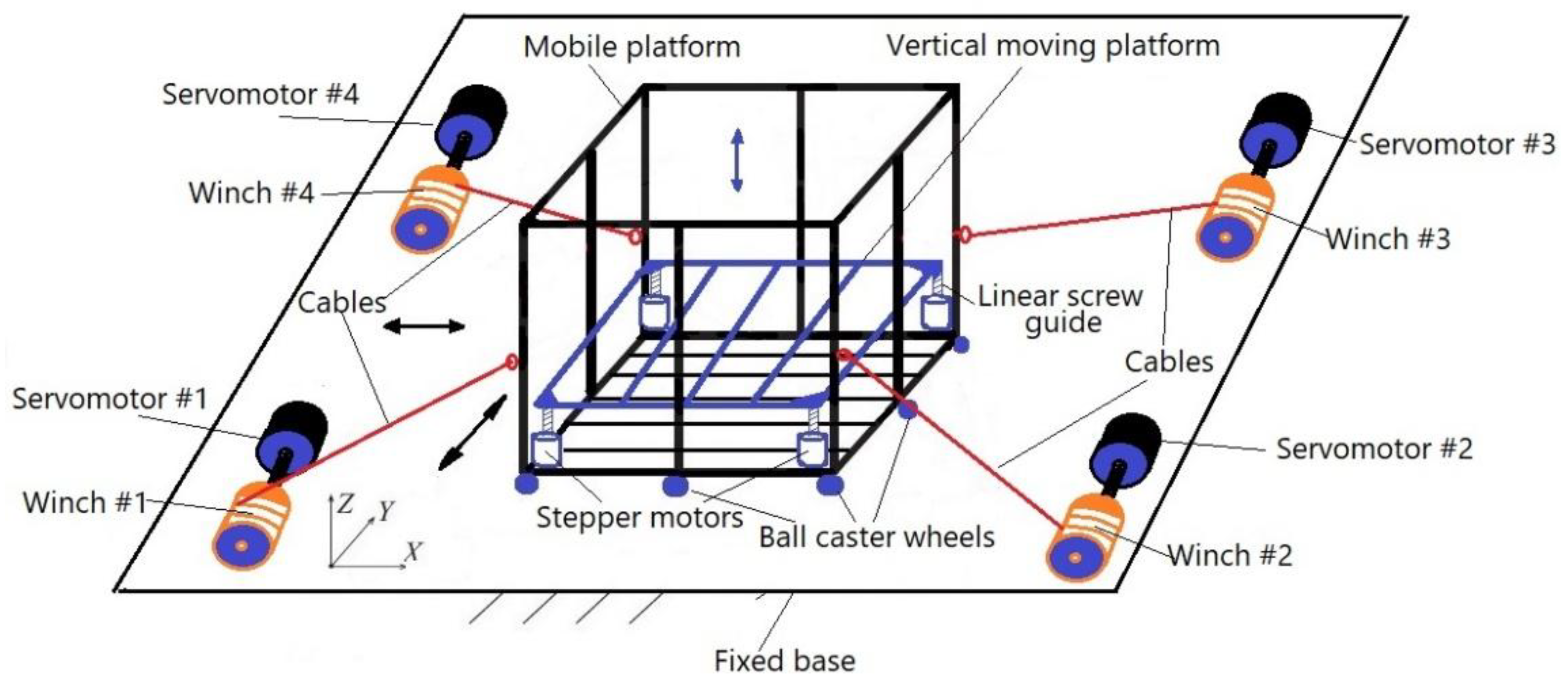
Figure 3.
Kinematic scheme of the CDPR.
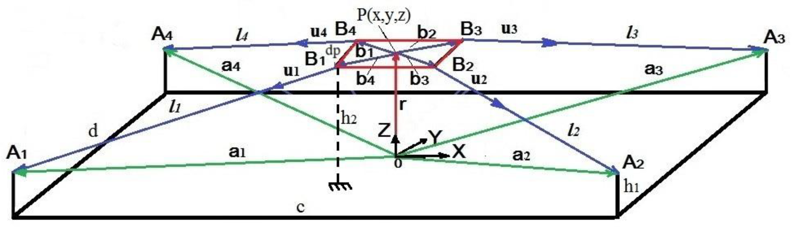
Figure 4.
Scheme of forces acting on the CDPR mobile platform.
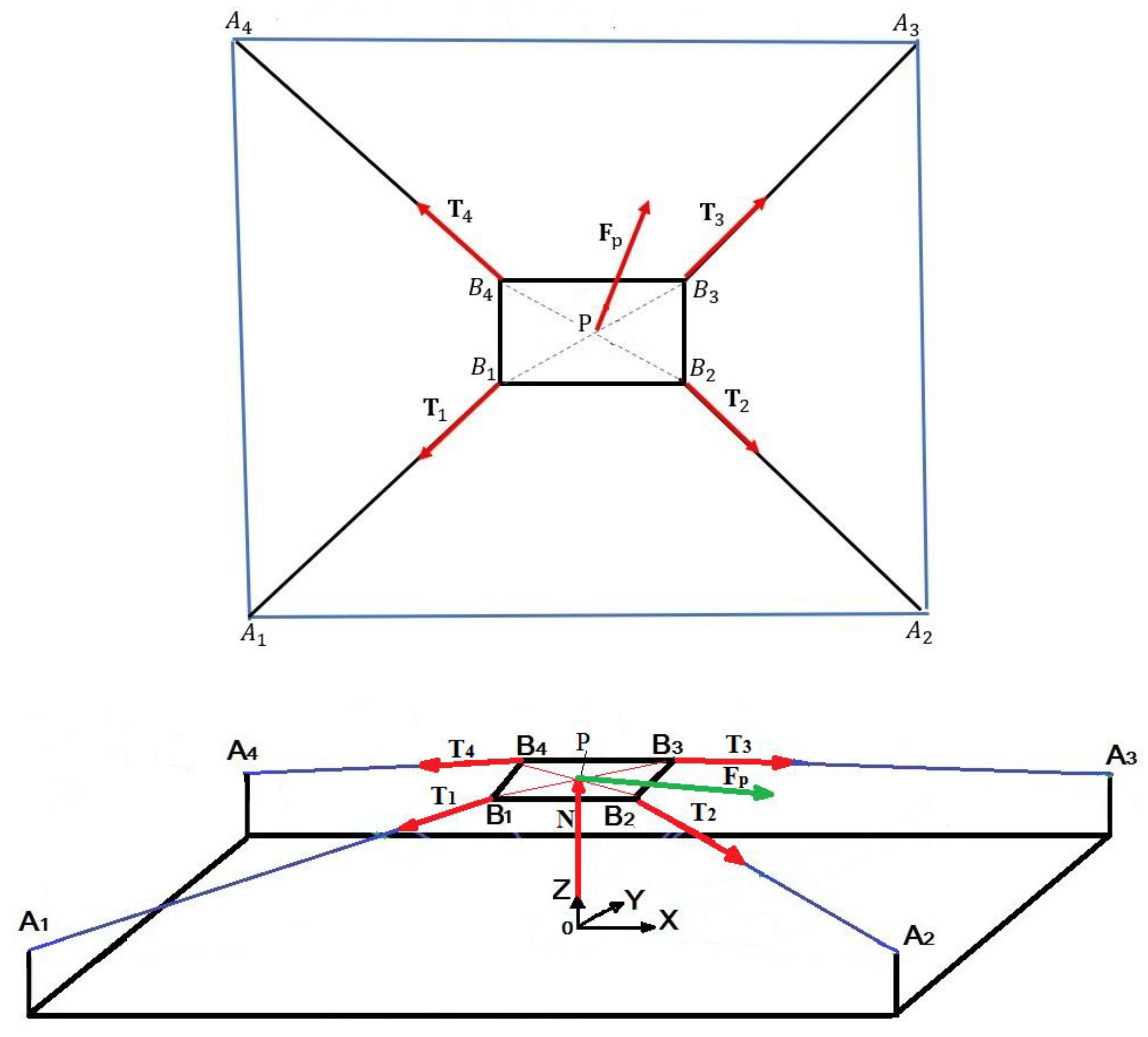
Figure 5.
Scheme of the action of forces for a CDPR with a purely translational motion. of the movable platform.
Figure 5.
Scheme of the action of forces for a CDPR with a purely translational motion. of the movable platform.
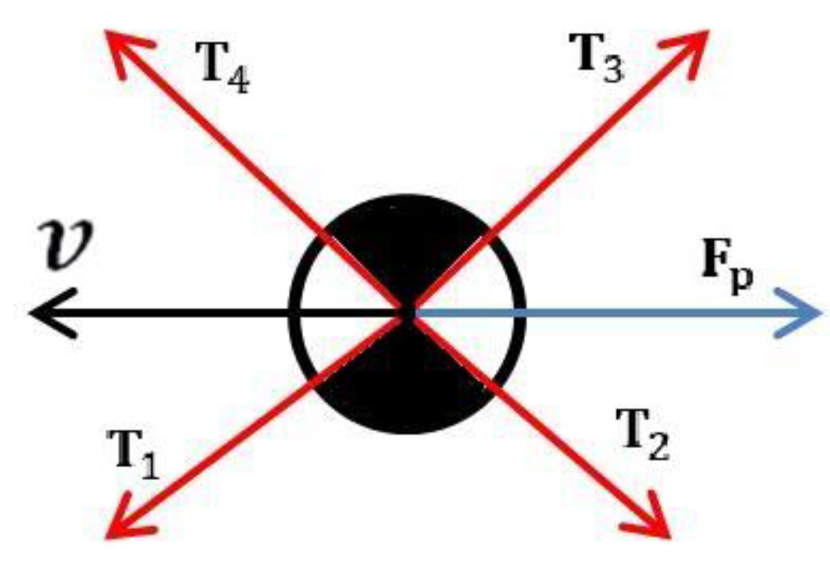
Figure 6.
Dynamic model for the servomotor shaft and cable winch drum.
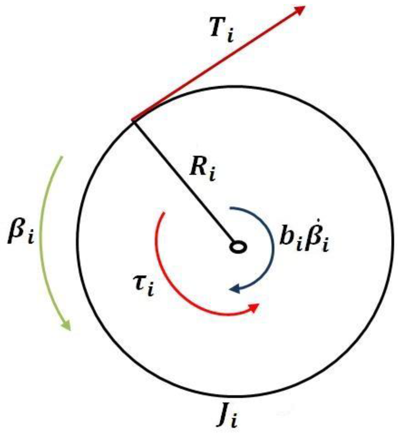
Figure 7.
A ball screw linear actuator.
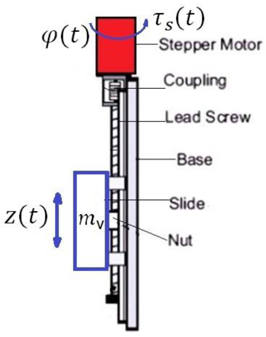
Figure 8.
The designed control scheme of the CDPR.
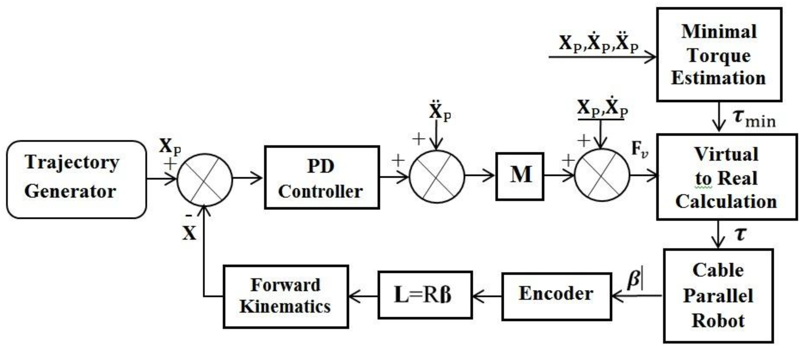
Figure 9.
Design of the prototype earthquake simulator a) horizontal motion unit, b) vertical motion unit.
Figure 9.
Design of the prototype earthquake simulator a) horizontal motion unit, b) vertical motion unit.
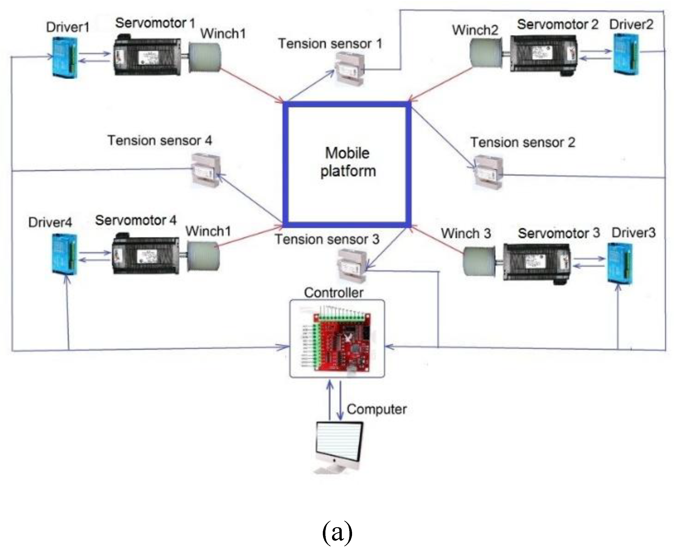
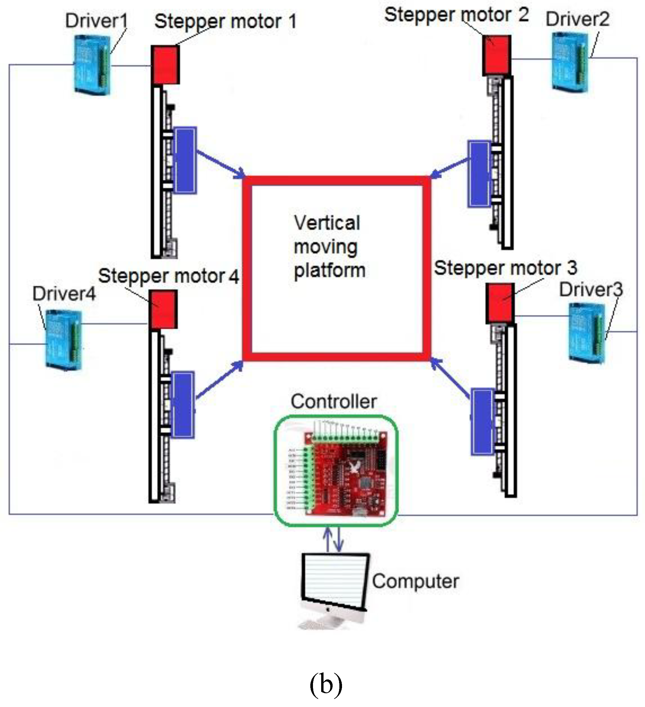
Figure 10.
Prototype of designed Earthquake simulator in Figure 9.
Figure 10.
Prototype of designed Earthquake simulator in Figure 9.
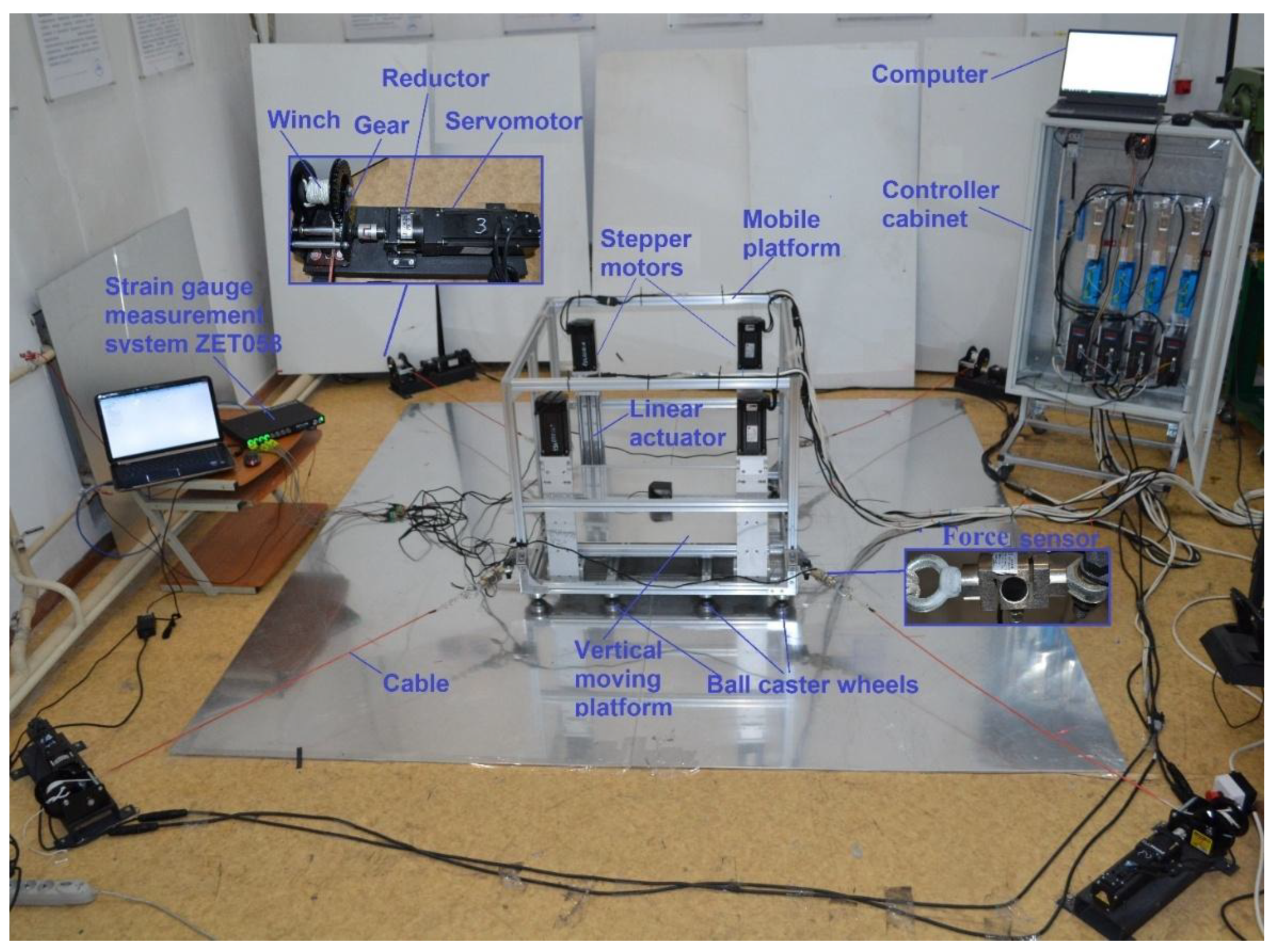
Figure 11.
Interface of the program for controlling the operation of the earthquake simulator prototype in Figure 9 and Figure 10.
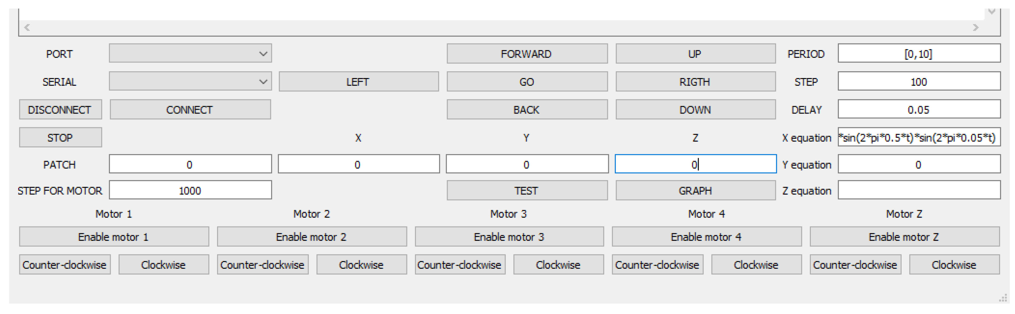
Figure 12.
Measurements of the platform trajectory in X direction using the rope displacement sensor.
Figure 12.
Measurements of the platform trajectory in X direction using the rope displacement sensor.
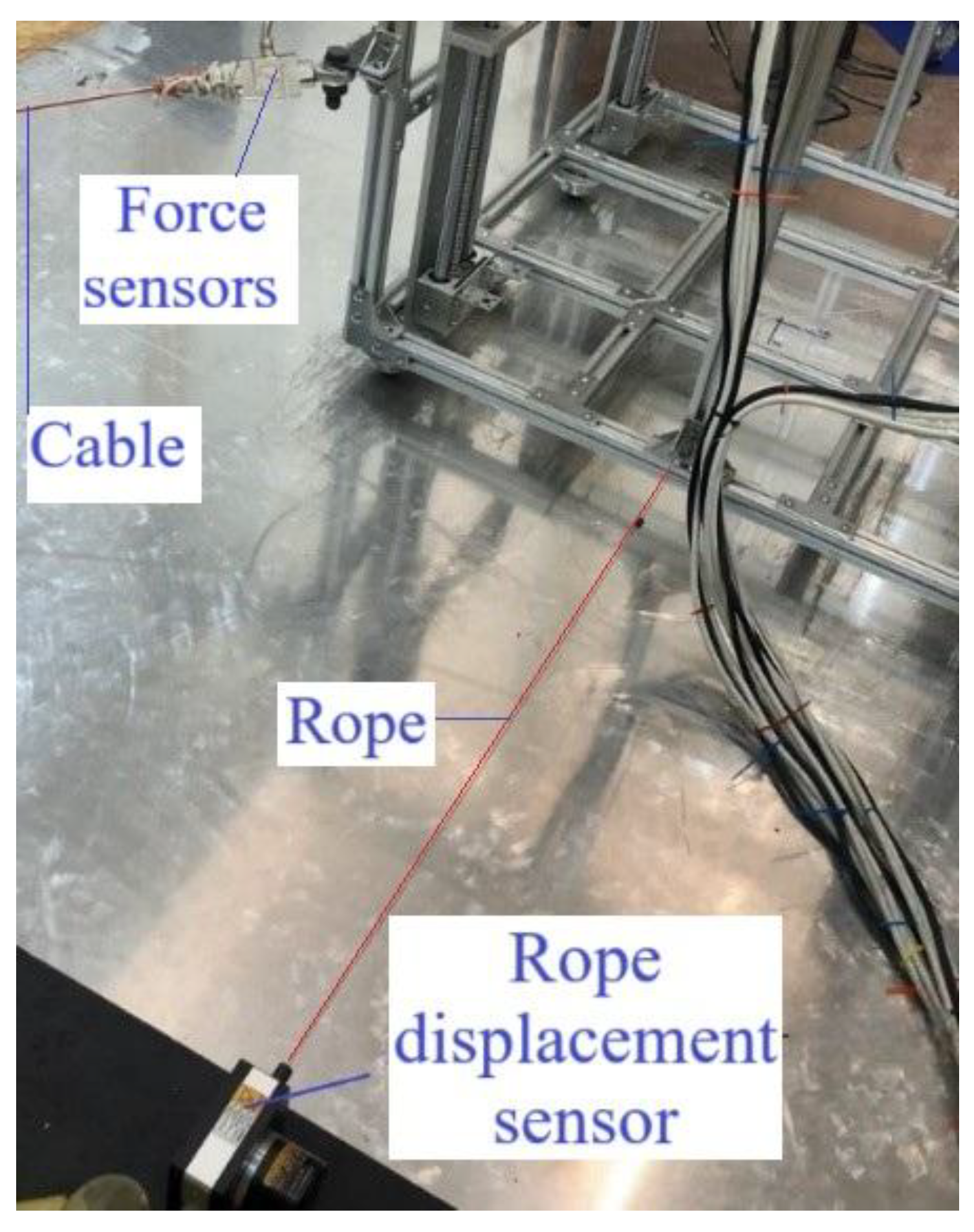
Figure 13.
Desired, measured and error trajectories of the platform motion.
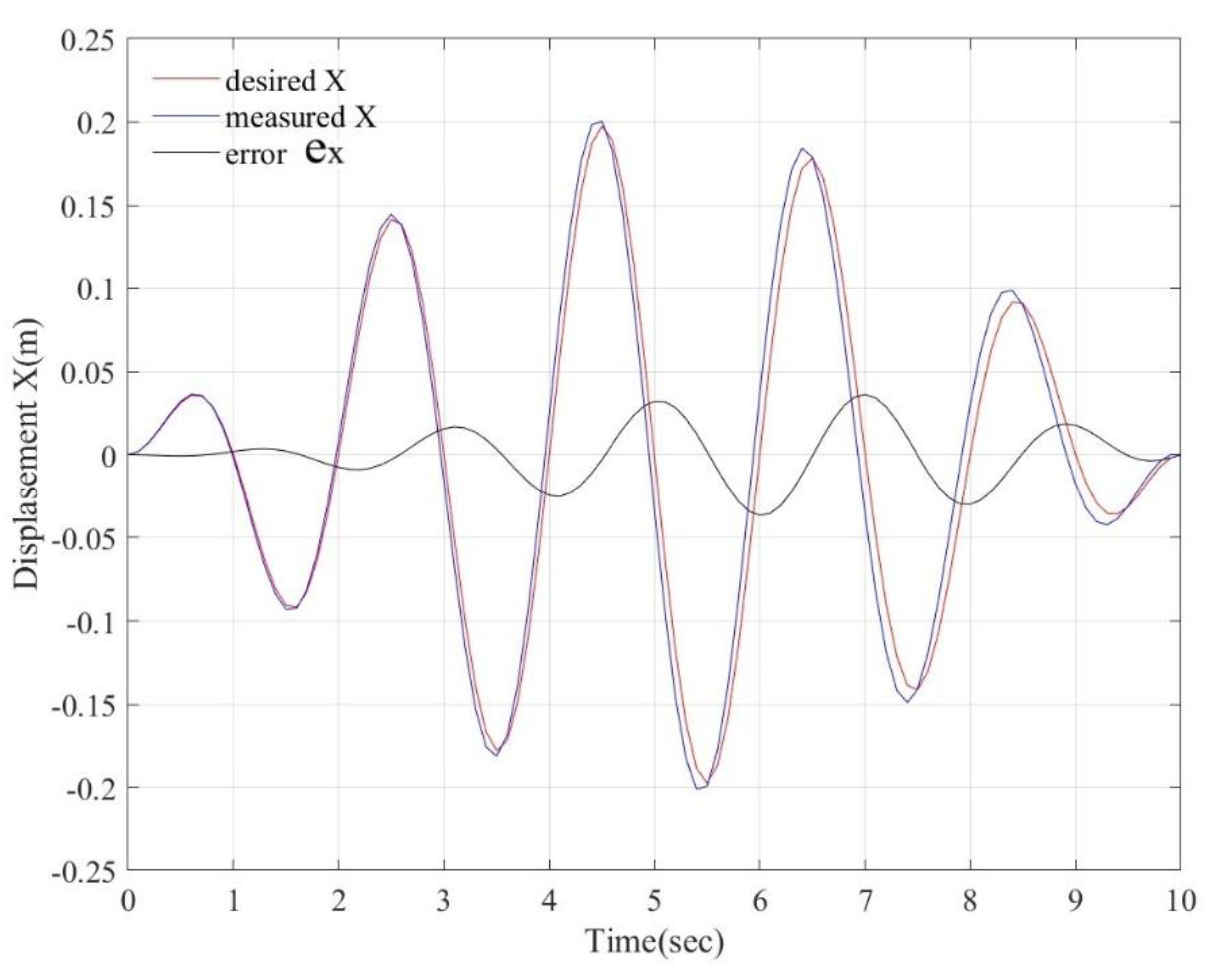
Figure 14.
Acquired data for a test with sinusoidal motion of the platform acceleration in the X-axis direction: a) desired and measured, b) desired and filtered measured.
Figure 14.
Acquired data for a test with sinusoidal motion of the platform acceleration in the X-axis direction: a) desired and measured, b) desired and filtered measured.
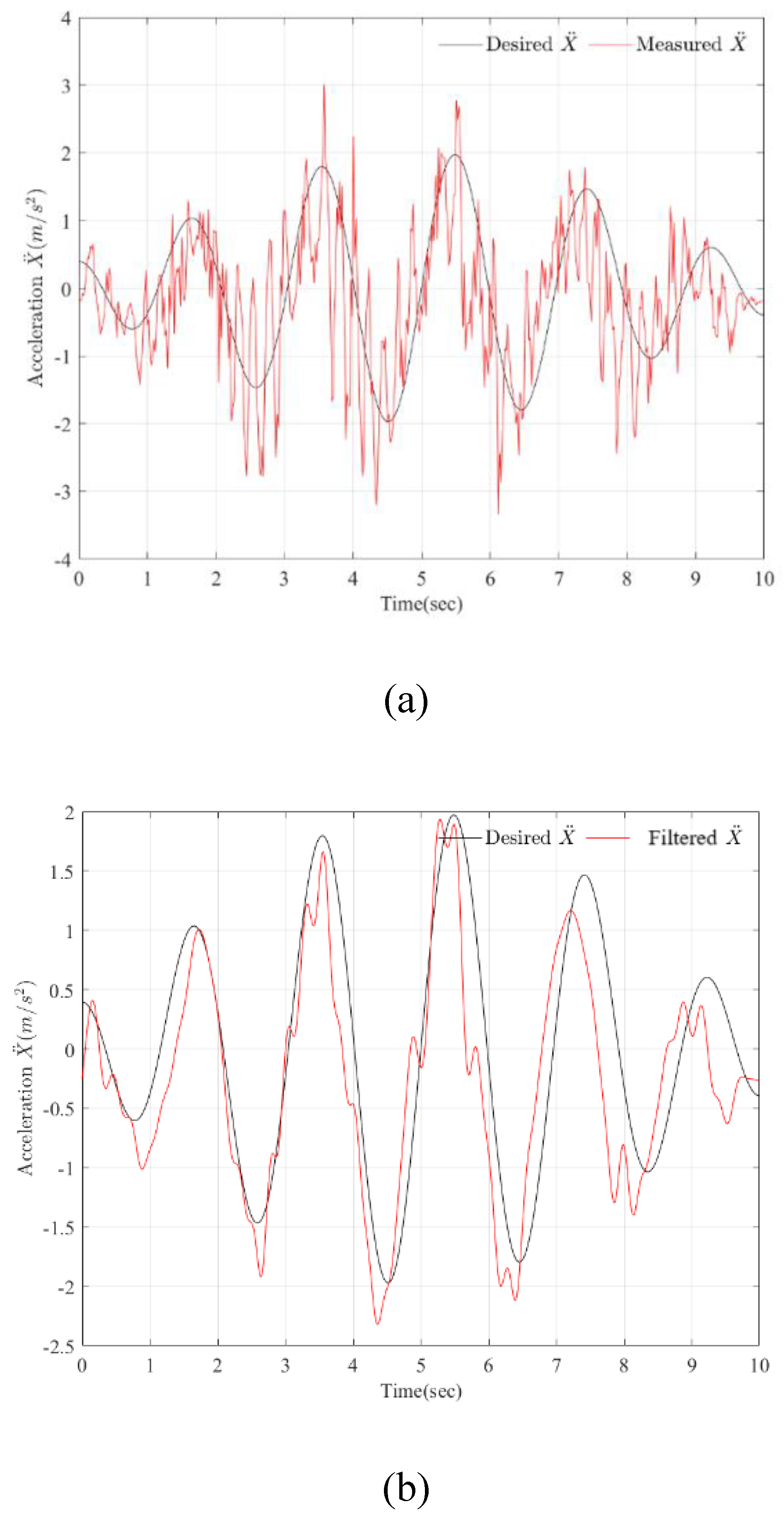
Figure 15.
CDPR cable tensions during movement in the direction of the X-axis.
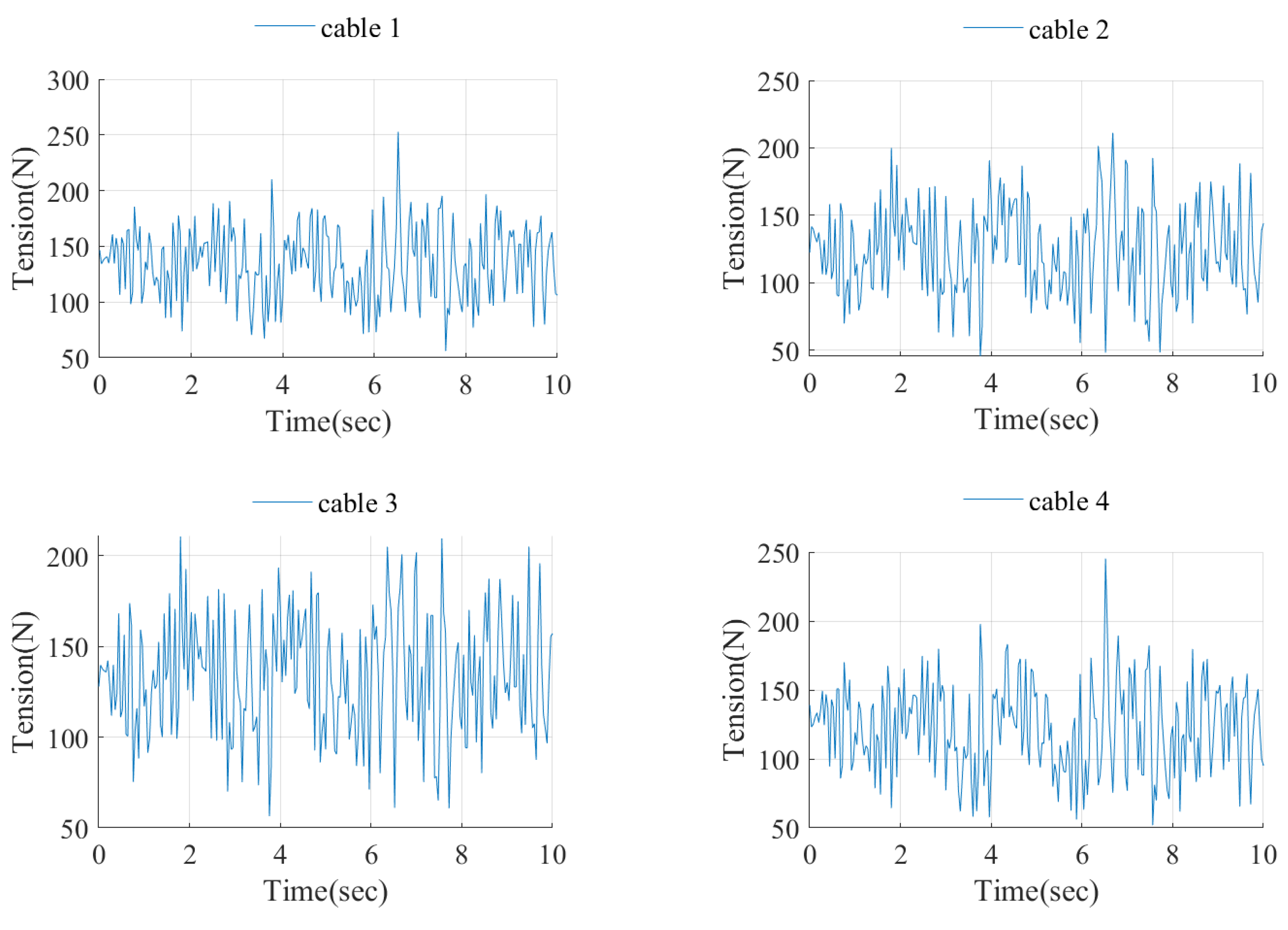
Figure 16.
Desired and measured trajectories of the platform motion.
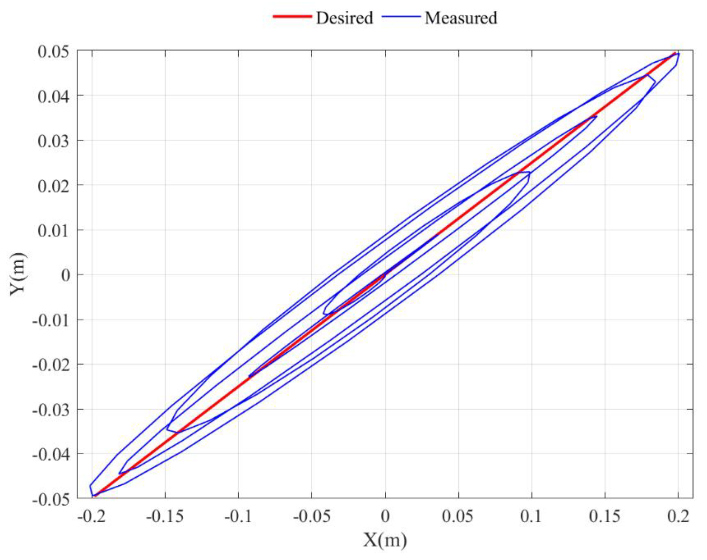
Figure 17.
CDPR cable tensions when the platform moves diagonally to the X and Y axes.
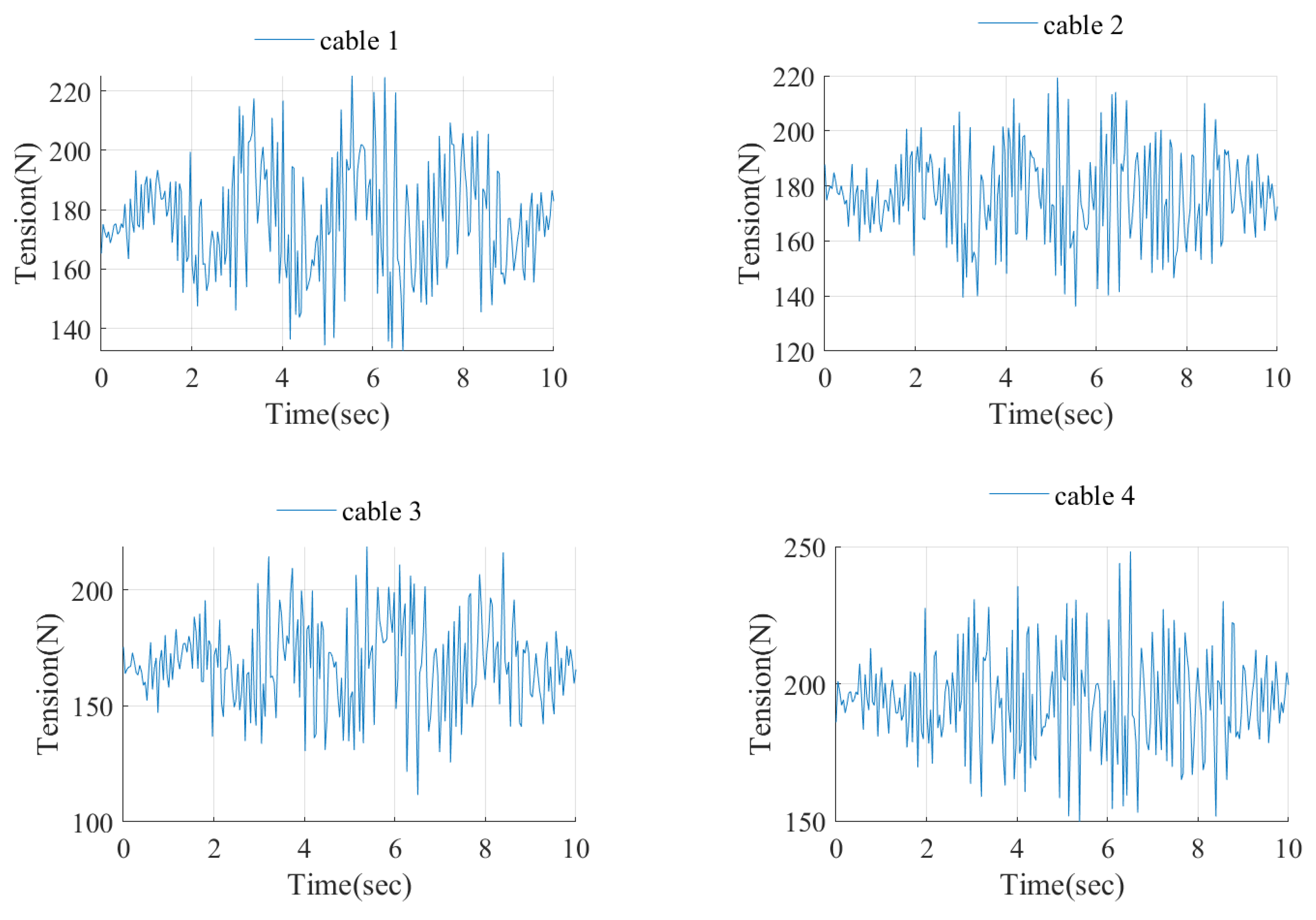
Figure 18.
Desired, measured and error trajectories of the platform motion in the direction of motion along the Z axis.
Figure 18.
Desired, measured and error trajectories of the platform motion in the direction of motion along the Z axis.
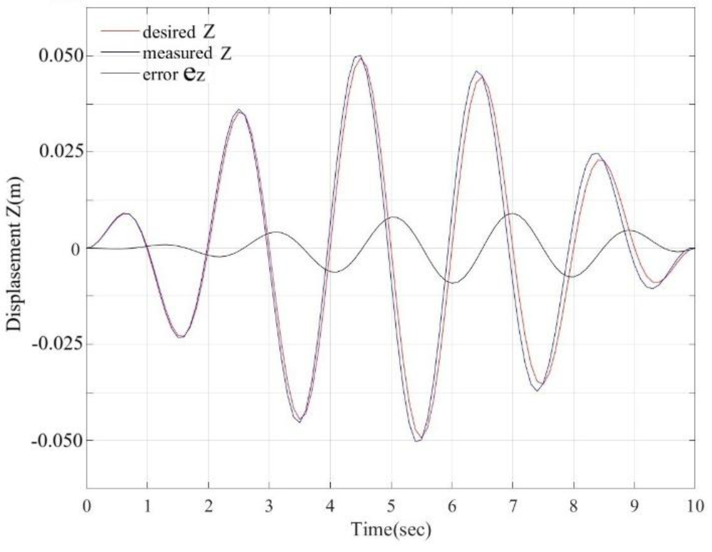
Figure 19.
Desired and measured acceleration of the platform in the direction of the Z axis.
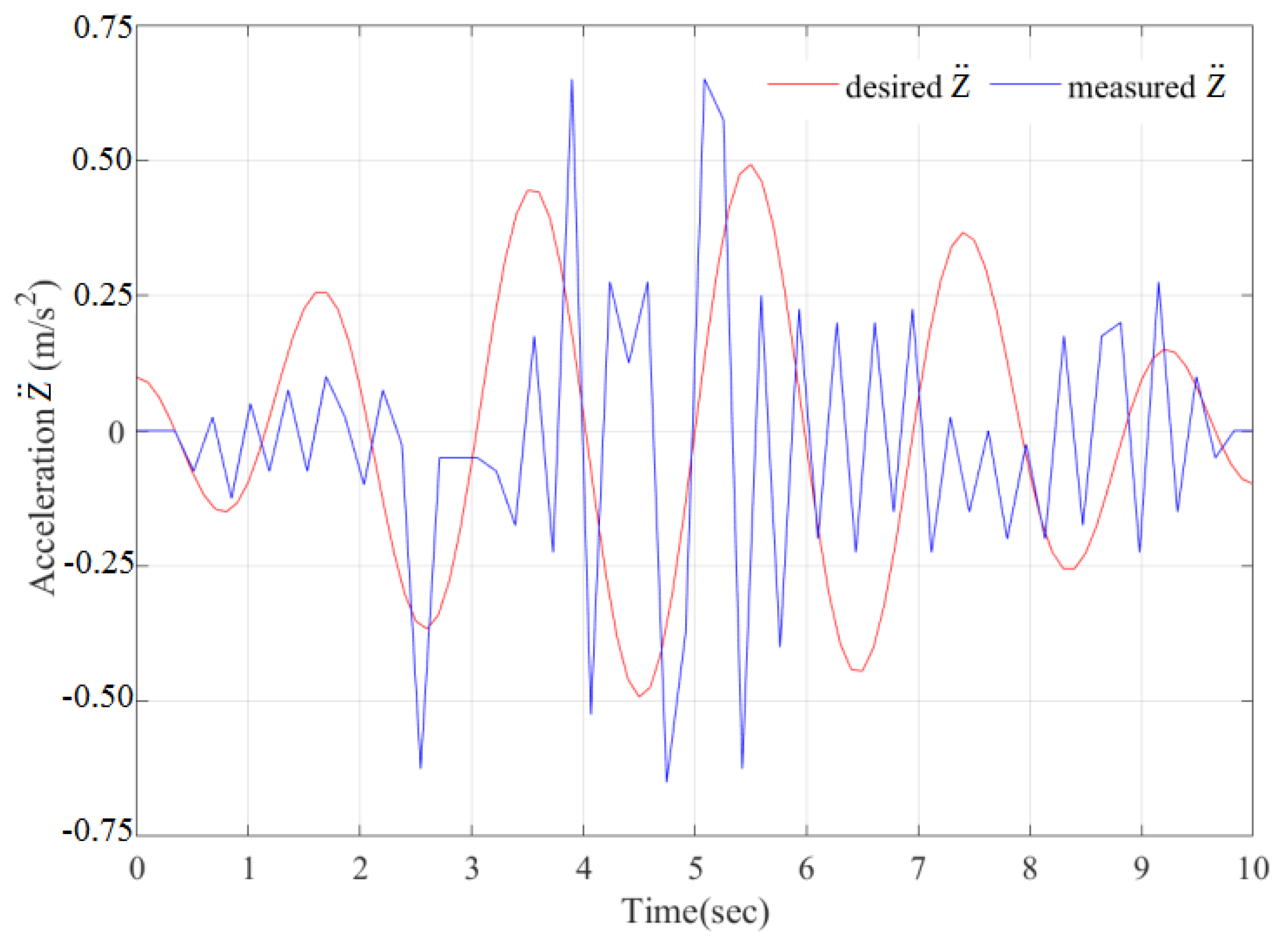
Figure 20.
A real seismogram of the San Fernando earthquake near Pacoima Dam, California, in 1971 [30]: a) Displacement; b) Velocity; c) Acceleration.
Figure 20.
A real seismogram of the San Fernando earthquake near Pacoima Dam, California, in 1971 [30]: a) Displacement; b) Velocity; c) Acceleration.
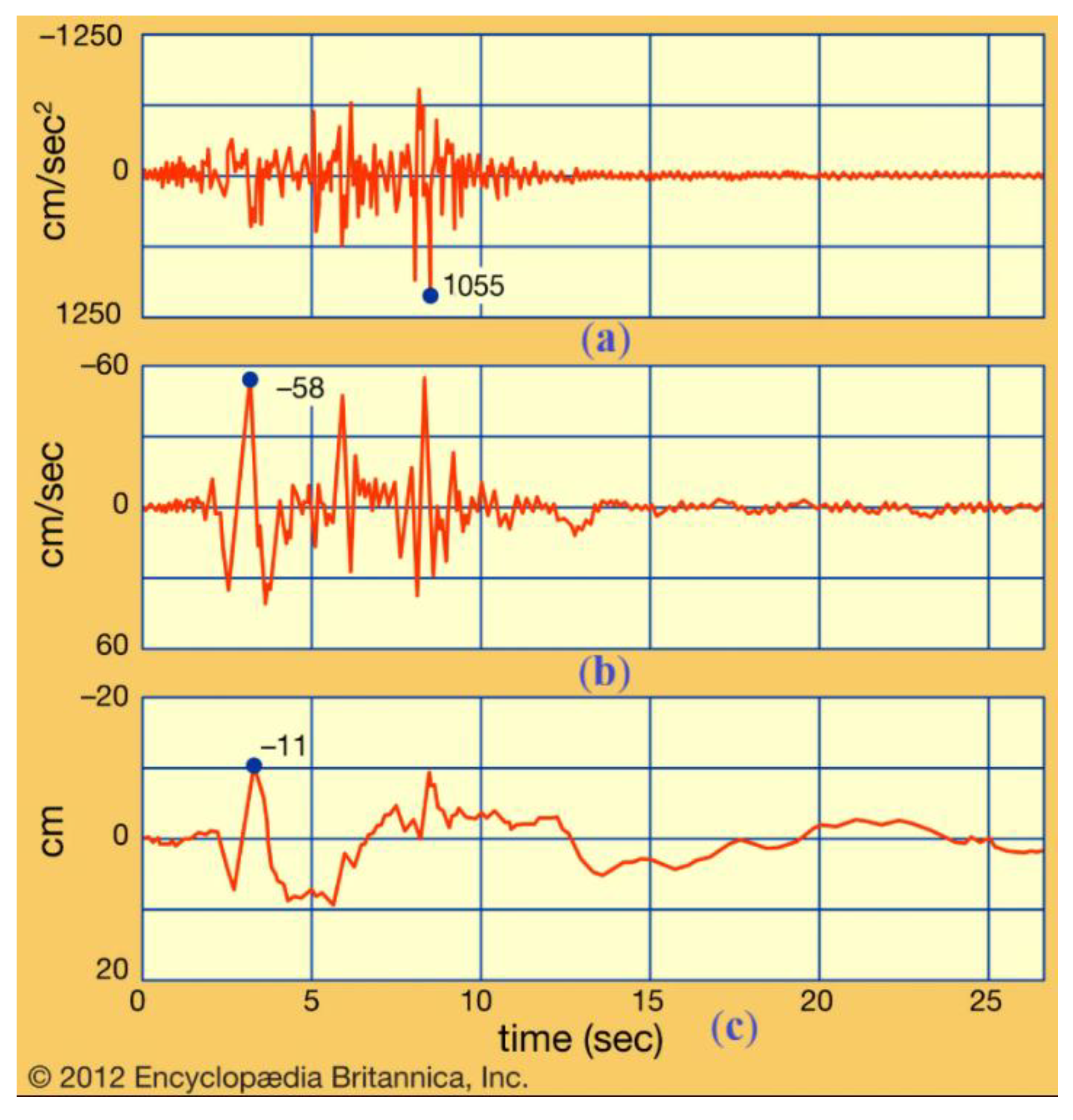
Figure 21.
Graphs of the CDPR cable lengths.
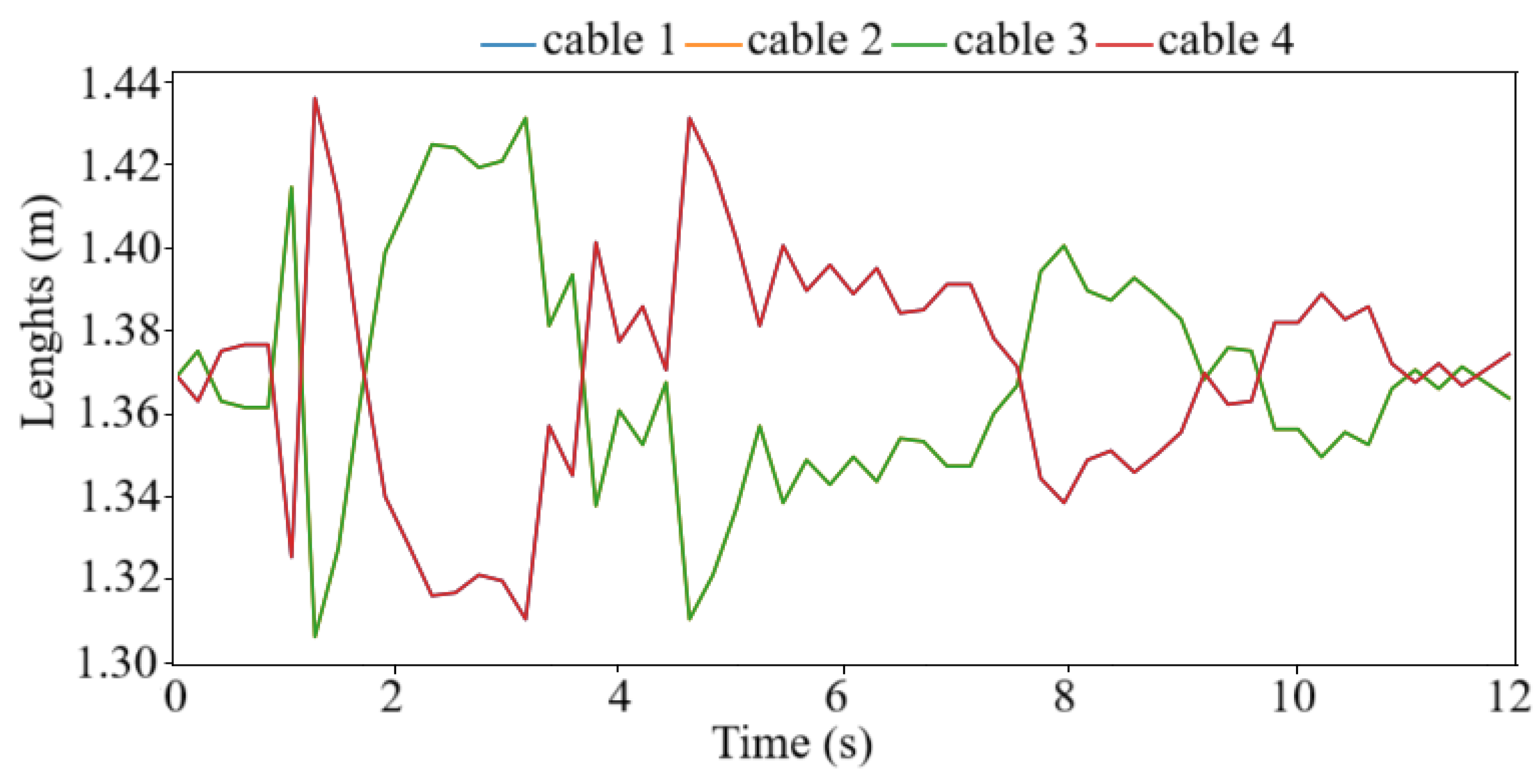
Figure 22.
Desired, measured and error displacements of the platform according to the real seismogram of the San Fernando earthquake.
Figure 22.
Desired, measured and error displacements of the platform according to the real seismogram of the San Fernando earthquake.
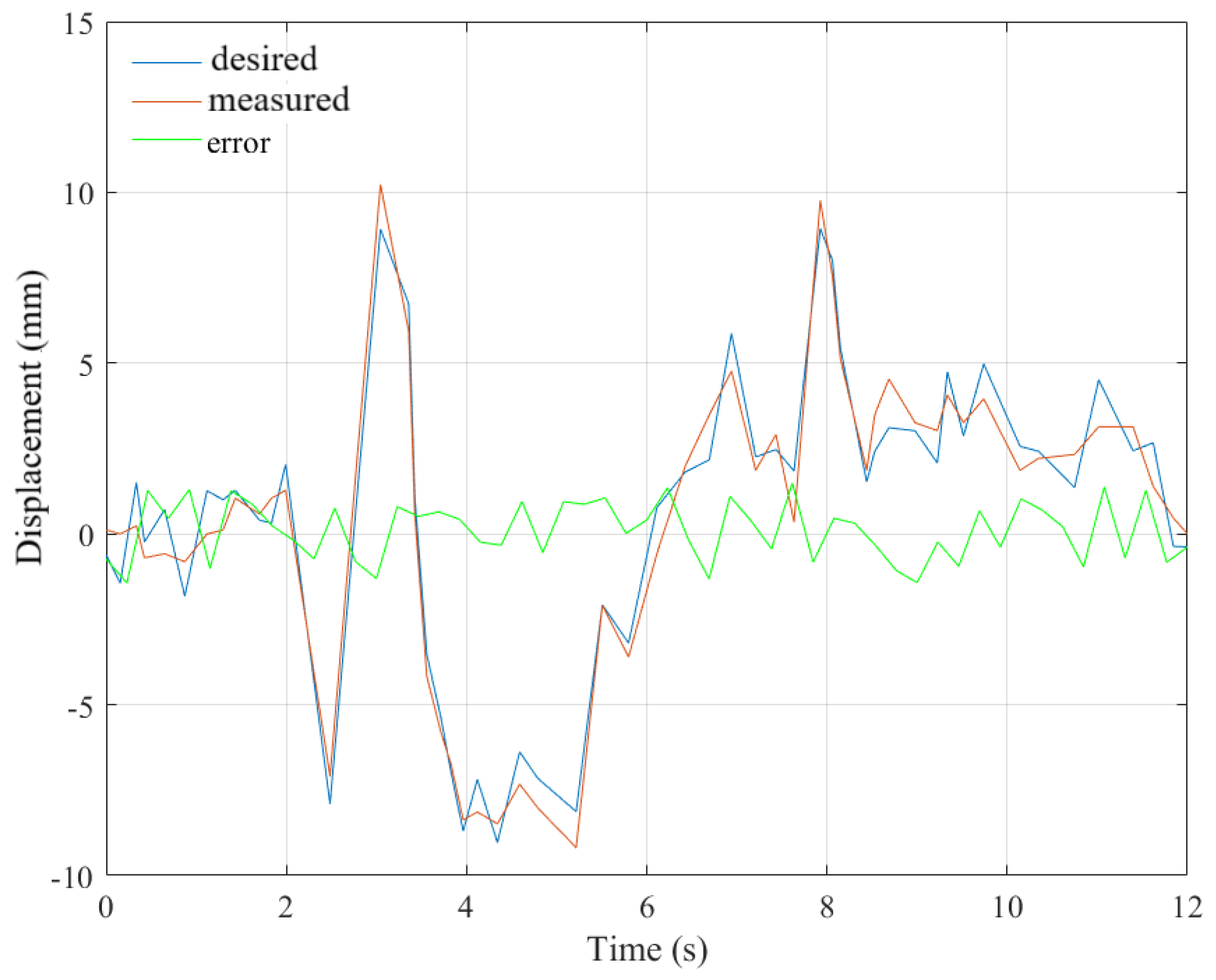
Figure 23.
Desired, measured accelerations of the platform according to the real seismogram of the San Fernando earthquake.
Figure 23.
Desired, measured accelerations of the platform according to the real seismogram of the San Fernando earthquake.
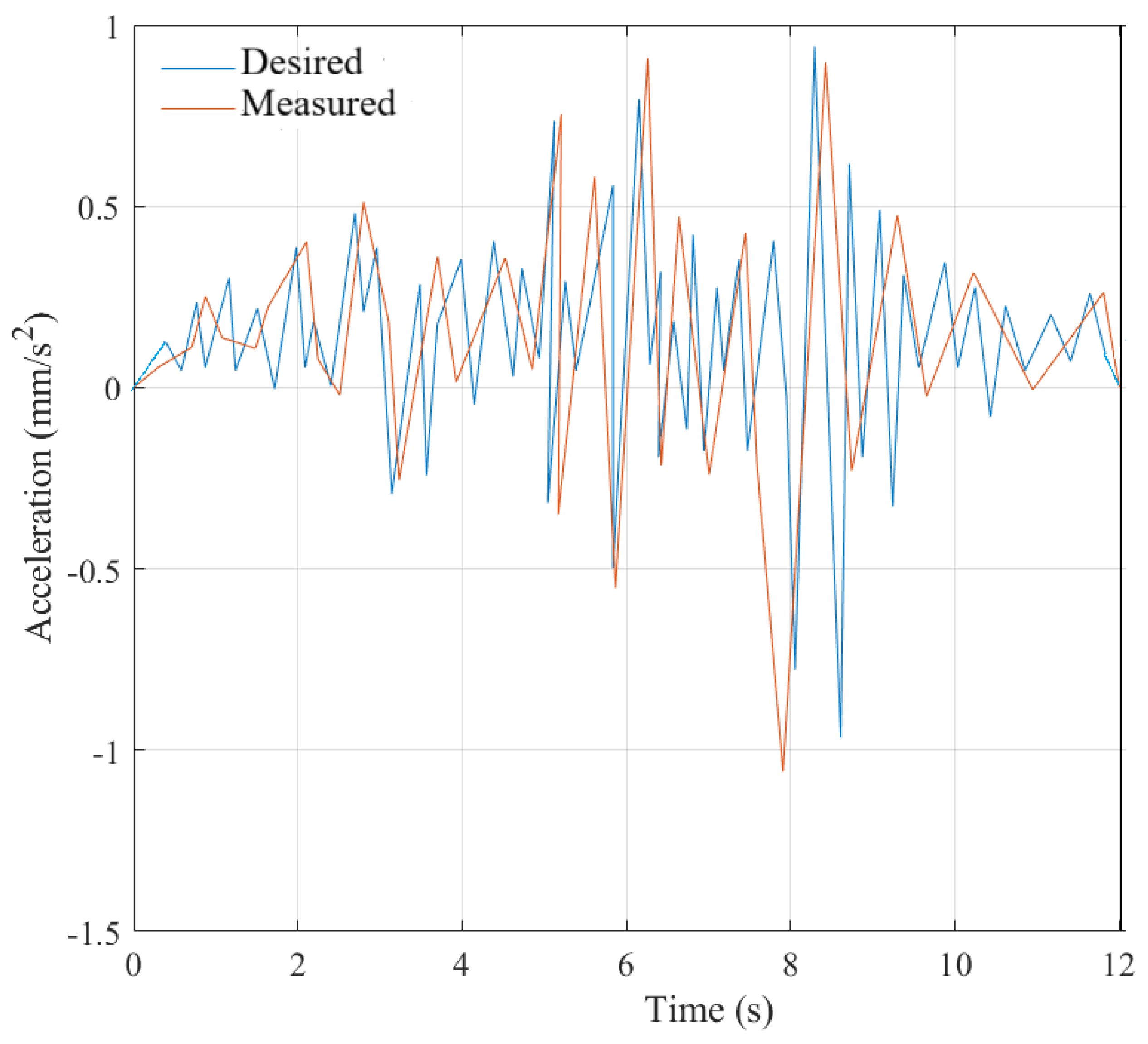

Table 1.
The coordinates of the vector can be expressed as.
| Cable i | |||
|---|---|---|---|
| x | y | z | |
| 1 | -c/2 | -d/2 | h1 |
| 2 | c/2 | -d/2 | h1 |
| 3 | c/2 | d/2 | h1 |
| 4 | -c/2 | d/2 | h1 |
Table 2.
The coordinates of the vector
| Cable i | |||
|---|---|---|---|
| x | y | z | |
| 1 | - dp/2 | -dp/2 | h2 |
| 2 | dp/2 | - dp/2 | h2 |
| 3 | dp/2 | dp/2 | h2 |
| 4 | -dp/2 | dp/2 | h2 |
Disclaimer/Publisher’s Note: The statements, opinions and data contained in all publications are solely those of the individual author(s) and contributor(s) and not of MDPI and/or the editor(s). MDPI and/or the editor(s) disclaim responsibility for any injury to people or property resulting from any ideas, methods, instructions or products referred to in the content. |
© 2025 by the authors. Licensee MDPI, Basel, Switzerland. This article is an open access article distributed under the terms and conditions of the Creative Commons Attribution (CC BY) license (http://creativecommons.org/licenses/by/4.0/).
Copyright: This open access article is published under a Creative Commons CC BY 4.0 license, which permit the free download, distribution, and reuse, provided that the author and preprint are cited in any reuse.


