Submitted:
24 September 2025
Posted:
26 September 2025
You are already at the latest version
Abstract
The paper gives a formulation of Thales' theorem that enables the definition of segment multiplication by avoiding the explicit connection to parallelism. This simplifies the approach to segment multiplication given in Hilbert's Grundlagen der Geometrie, which is based on Pascal's theorem. Moreover, it suggests an idea of equiangularity that provides a more general formulation of many theorems independently of the different Euclidean or non-Euclidean settings. The relationship of Thales' theorem with other important theorems, and with incommensurability, is considered, which illuminates its cruciality in the organization of Euclid's Elements.
Keywords:
Thales theorem
; segment multiplication
; parallel axiom
; non-euclidean geometry
1. Introduction
Thales’ theorem (VI century B.C.), in one of its usual formulations, says that given two lines having a common point A, when intersected by two parallel lines, they determine correspondent segments over them: and , respectively, that are in the same ratio: .
It is one of the oldest achievements in Greek geometry. Thales did not prove it, but used it for evaluating distances by angles, as it will clearly appear from the definitions that we give of segment multiplication. It is a formidable method for evaluating great distances (Eratosthenes used it to calculate Earth’s circumference). Later, Thales’ intuition was transformed into a theorem on segment proportions. Euclid postpones it to the sixth book of his thirteen books of Elements [3] (Proposition VI, 2). Namely, the proof is simple when corresponding segments have a rational ratio; if they are not commensurable, then very often certain kinds of arguments require some forms of Eudoxus’ hexaustion method, considering infinite sequences of rational ratios (Euclid VI, 1 in [3] and Proposition III, 3 in [8]). Segment multiplication is a key point in Hilbert’s book on the foundations of geometry [5]. In this paper, we consider a segment multiplication based on a particular case of Thales’ theorem, from which the general case easily follows. Then, the “correctness" of this segment multiplication is proved, and Thales’ theorem is related to the parallel axiom and to other fundamental concepts and theorems of Euclidean geometry.
2. Segment Multiplication
In Grundlagen der Geometrie [5], a classic book on the foundations of geometry (the first edition in 1899, the last one in 1971), Hilbert reformulates the theory of proportions of Euclidean geometry in equational form by defining the sum and product of segments. Figure 1 illustrates Hilbert’s definition of multiplication between two segments. It is based on parallel lines, but the proof that his segment multiplication is correct, that is, satisfies all the properties of multiplication on real numbers, is given by using a particular form of a theorem proved by Blaise Pascal in the context of the conic section curves [5].
Let us provide a different definition of segment multiplication related to Thales’ theorem. In the following, a line will always be considered a straight line. Let be an angle of two half-lines with common origin A. Let P be any point of and , the point where the orthogonal line to in P intersects . We denote by this orthogonal correspondence, omitting the subscript when it is arguable by the context. If , with unitary segment, and X a point in , we set (see Figure 2), and the orthogonal multiplication of by is given by:
The following algorithm computes the orthogonal segment multiplication.
Thales’ Orthogonal Multiplication Algorithm
1. Let be two numbers for which has to be calculated, and a fixed unitary length;
2. Let be the points on a half-line r with origin A, such that have lengths ;
3. Let H be any point on r before P, draw the line h orthogonal to r in H;
4. Let be the point of h such that (, , and );
5. Let be the point on the line such that , then .
Remark 2.1.
In the previous algorithm, the angle is constructed such that the length of provides ab. Alternatively, we can fix an angle and determine the point X of such that has length a. Then, we search for the point of such that: 1) X is in , 2) , and 3) has length b. This point provides the segment of length ab. The two methods correspond to different choices of the unitary length.
Now we state the orthogonal version of Thales’ theorem as a direct consequence of orthogonal segment multiplication. Let us define the length multiplication of a segment s by a number k, denoted by , as the segment such that , where l is a function from segments to numbers giving the length (with respect to a unitary segment 1). The existence of a length function with this property is not obvious. Namely, it means that segments with length multiplication satisfy the Archimedean axiom (Euclid X, 1), holding on real numbers (given two numbers , there always exists a positive integer such that ). This means that if , then , for some positive integer n.
Segments are identified by their length and extremities, which may change when they are moved. For this reason, very often, when no confusion can arise, segments and lengths (numbers) are denoted in the same way.
Theorem 2.2
(Thales VI B.C., orthogonal version). Given an angle , for any pair of segments of , respectively:
Proof.
According to the definition of , in the correspondence holds. By the definition of segment length multiplication, the ratio between the lengths of two segments does not change if they are multiplied by the same number, that is, . Therefore, changing the unitary length by a suitable factor , from we derive , that is, with . Whence, , and . □
Remark 2.3.
According to the previous theorem, in an angle , the ratio between the lengths of orthogonally corresponding segments is always the same. This implies that the angle intrinsically determines the number independently of any choice of the unitary length. Therefore, a “poetic" formulation of Thales’ theorem could be: Angles are pure numbers. □
Theorem 2.4.
The segment multiplication commutes with the length function l:
Proof.
According to the proof of the previous theorem, for a suitable angle such that : , therefore □
The previous theorem tells us that Thales’ orthogonal theorem can be paraphrased by saying that the orthogonal segment multiplication coincides with the segment length multiplication, or equivalently, that, for any angle and number k, the orthogonal correspondence preserves the segment length multiplication:
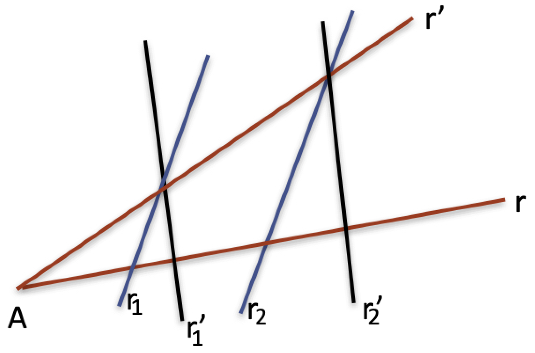
In general, Thales’ theorem is formulated in terms of parallel lines that are not necessarily orthogonal to one line of the angle. However, this more general formulation follows directly from the orthogonal version of the theorem by combining two applications of the orthogonal version. Figure 3 suggests clearly how to do it (the ratio between segments of lines with can be obtained from the ratios of with and . The formulation based on orthogonality also has the advantage of being generalized to non-Euclidean geometries, as we suggest in a following section.
Thales’ theorem, in its general form, can be inverted, as shown by the following theorem.
Theorem 2.5.
If the lines and of angle are cut by two distinct lines producing on them corresponding segments that are in the same ratio, then lines r and are parallel.
Proof.
Lines can join outside of the angle either externally to or externally to (otherwise ). Let be the line where no intersection external to exists. Then, reporting the angle by the line , such that , we should have on corresponding segments that are equal to those formed on ; therefore, if join externally to , they also join externally to against the hypothesis. □
Figure 3.
Thales’ theorem obtained from its orthogonal version.
According to Theorem 2.4, segment orthogonal multiplication is commutative, associative, and distributive with respect to the segment addition.
Theorem 2.6.
The orthogonal segment multiplication is correct and complete with respect to number multiplication.
Proof.
Completeness follows when we assume the completeness of line: any real number x corresponds to a point such that, if we fix a point A in r, then , where 1 is a unitary segment. □
Hilbert in [5] states the continuity of lines by using a completeness axiom that is more properly a meta-axiom, stating that no other system of axioms can exist that extends to a wider class of geometrical entities the properties following from the other 19 axioms (divided into five groups: Axioms of connection, Axioms of order, Axiom of parallels, Axioms of congruence, Archimedes’s axiom). Euclid investigates continuity in Book X on commensurability and uncommensurability. Modern classical approaches to continuity are due to Augustine Cauchy, Kari Weierstrass, Richard Dedekind, and Georg Cantor. They are all strictly related, in analytical or algebraic settings, to Eudoxus’ hexaustion method, on which Euclid builds his arguments, widely used and extended by Archimedes [3,4]. However, the birth of differential analysis, since its prodromes (related to Archimedes’ Method), before Newton and Leibniz (Bonaventura Cavalieri, Pierre de Fermat, Evangelista Torricelli, John Wallis, Blaise Pascal, Christiaan Huygens, James Gregory) belongs to an interrupted line of thought strictly related to continuity and incommensurability [7].
For Greeks, the completeness of lines was an implicit assumption, because they identified numbers with ratios of segments. The discovery of pairs of segments with ratios that are not fractions was the origin of the difficulty in stating general assertions about ratios between segments. For this reason, Euclid postpones proportions to the end of the geometry of the plane.
3. Euclid’s and Pythagoras’ Theorems on Right Triangles
Euclid’s first theorem on right triangles says that the square over a cathete is equal to the product of the hypotenuse and the projection of a cathete over the hypotenuse (see Figure 4).
This theorem follows directly from Thales’ theorem, because if is the angle opposite to cathete b, and segments p, q the orthogonal projections of a and b in the hypotenuse, respectively, then and . Therefore, we derive , that is, .
From Euclid’s first theorem, we have , but even , therefore, summing:
This proof is reported by Erwin Schöredinger [11] as the shortest proof of Pythagoras’ theorem.
Figure 4.
Euclid’s first theorem: .
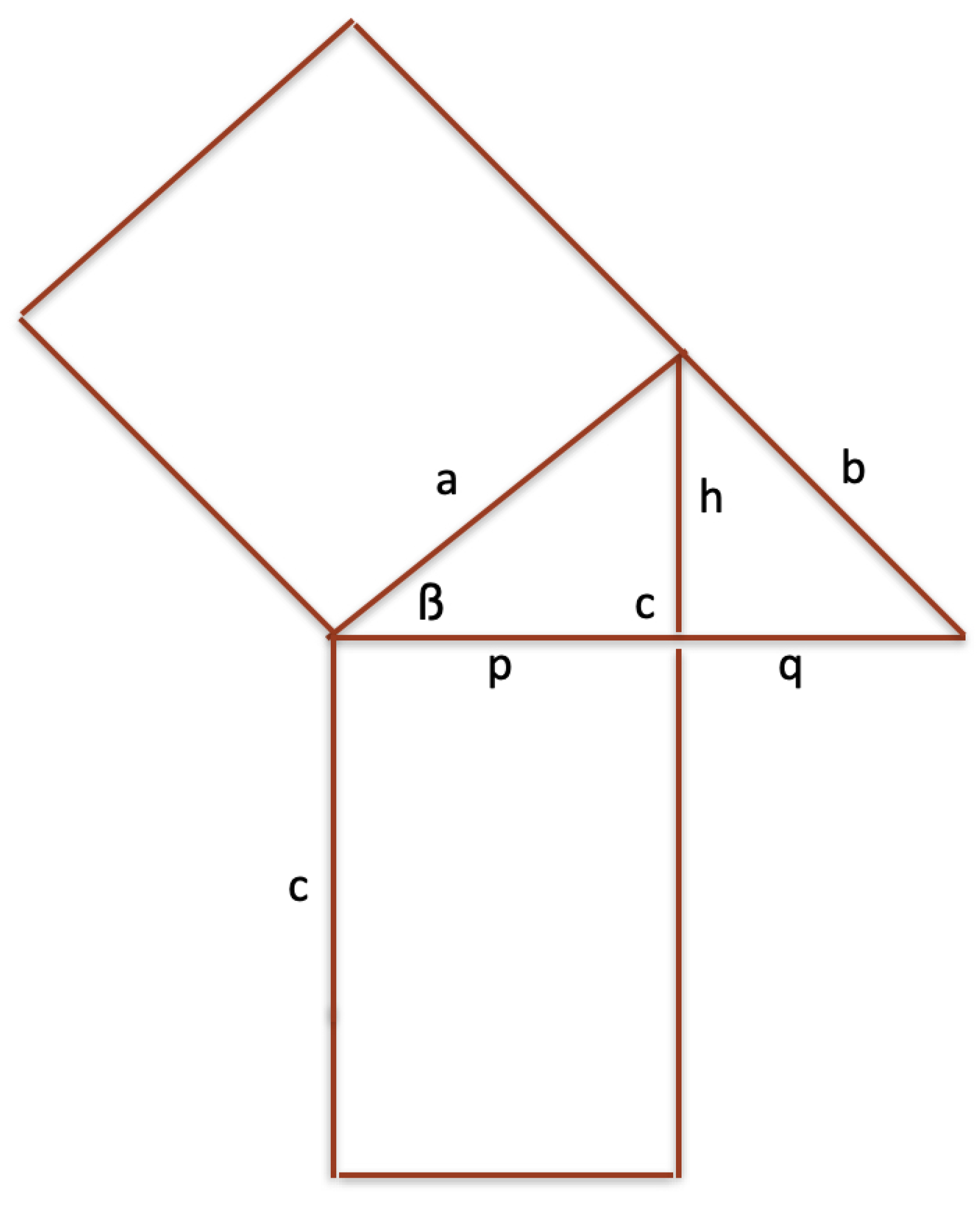
Euclid’s second theorem says that the square of the height with respect to the hypotenuse is equivalent to the rectangle of the two projections of the catheti over the hypotenuse. From Figure 5, it is easy to realize that the two angles marked by are equal (both summed to the angle give a right angle). Therefore, from Thales’ theorem, the equation follows, whence .
In conclusion, Euclid’s and Pythagoras’ theorems on right triangles directly follow from Thales’ theorem in orthogonal formulation.
Let us consider another segment multiplication defined over an angle , say it vertical multiplication, as indicated in Figure 6.
Theorem 3.1.
Vertical segment multiplication is equivalent to Hilbert’s segment multiplication, and it is also equivalent to the orthogonal multiplication.
Proof.
The first equivalence is proved by Figure 7. The second equivalence follows from Pythagoras’ according to which vertical segments are all in the ratio with the corresponding horizontal segments. □
At the end of the third chapter of [5], where Hilbert uses Pascal’s theorem for proving the correctness of his segment multiplication, from this correctness, he derives Thales’ theorem, which is called Fundamental theorem of proportions. Now we prove Pascal’s theorem by using Thales’ theorem. Parallelism between lines will be denoted by .
Theorem 3.2
(Pascal). Let be three points internal to the edge e of an angle , and be points internal to the edge f of angle (see Figure 8). If and , then .
Proof.
We mention that Paul Bernays, in his Second Supplement to [5], proves Thales’ theorem by using the incenters (where bisectors of a triangle meet, but an implicitly restricted form of Thales’ is used).
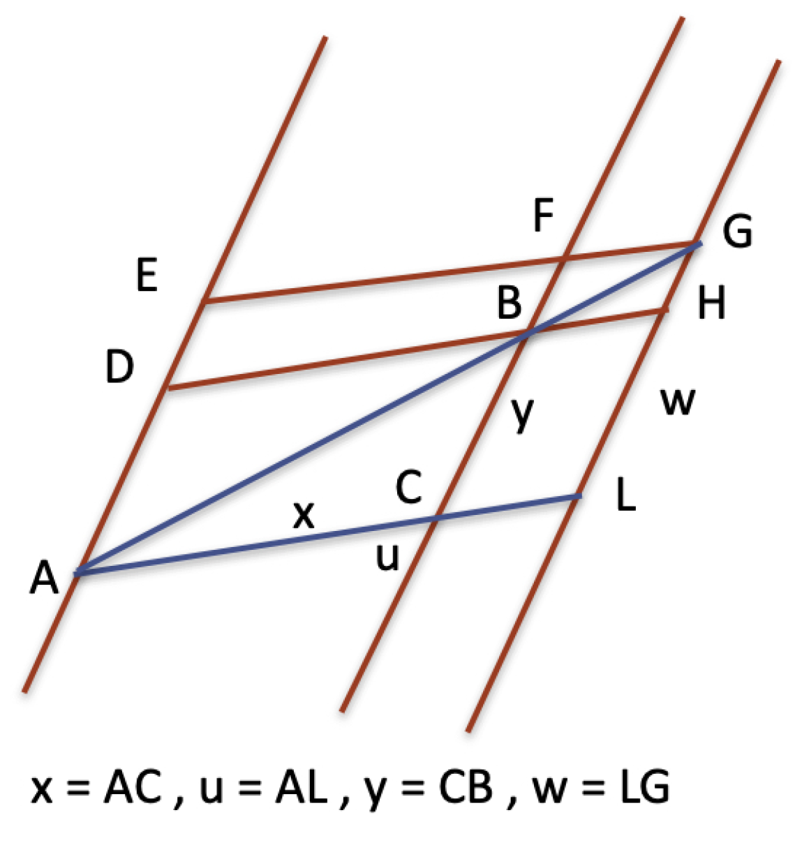
Finally, another theorem equivalent to Thales’ theorem is the Gnomon Theorem (Euclid I, 43), saying that in any parallelogram the complements about the diagonal are equal (see Figure 9). Namely, because they are the difference of equal triangles , . Then , therefore, , which implies Thales’ theorem .
4. Equiangularity
As we have already noticed, in the above orthogonal multiplications, we did not use parallel lines, but only orthogonality. This suggests to us a notion more general than parallelism. Two lines with a common point are equiangular when they form four equal angles. In Euclidean geometry, equiangular lines are orthogonal, and the angles they form are right angles. However, in the non-Euclidean geometries [2,6], orthogonality does not coincide with equiangularity, because two lines can form equal angles that are not right angles (see Figure 10). Equiangularity is important because it allows us to extend Thales’ angle multiplication to non-Euclidean geometries.
We say that a segment s of a line is equiangular with another line if is equiangular with . The following theorem gives a property of equiangularity that enables us to define a restricted form of parallelism.
Theorem 4.1.
A segment is equiangular with a line r if it is the shortest segment joining the point A with the line r. Conversely, the shortest segment joining A with r has to be equiangular with r.
Proof.
Only one equiangular segment can join A with r in the shortest way, because if A segment joins A with r and , triangle can be formed and , therefore the triangle is isoscele, therefore a point of the segment there exists that is shorter than and , then both these segments cannot be the shortest segments joining A with r. Conversely, if is the shortest segment joining P with r, then the line including has to be equiangular with r. Namely, if it forms with r angles that are not equal, then a triangle can be formed with placed in the smaller angle , and should be smaller than , against the hypothesis that is the shortest segment joining A with r. □
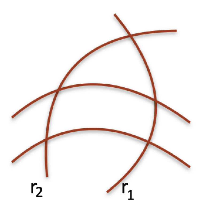
The notion of equiangularity enables us to extend the angle multiplication by using the equiangular correspondence in place of the orthogonal one. Moreover, we can introduce a notion weaker than parallelism. Two lines are quasi-parallel if a segment exists joining them that is equiangular with both lines. In this case, given a line r and a point A that does not belong to r, if with is the equiangular segment of r in P, the line r such that is equiangular with in A is the quasi-parallel to r including the point A. A “curve" version of Thales’ theorem can be developed in cases as shown in Figure 11.
Figure 10.
Equiangular and quasi-parallel (curve) lines in non-Euclidean geometries. The equiangular lines intersect by providing four angles that are not right angles.
Figure 10.
Equiangular and quasi-parallel (curve) lines in non-Euclidean geometries. The equiangular lines intersect by providing four angles that are not right angles.
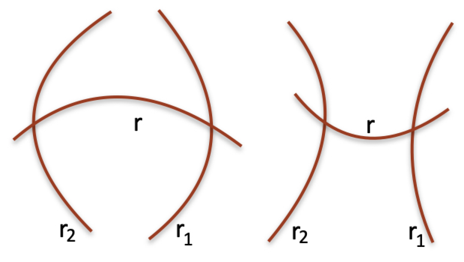
Figure 11.
Two quasi-parallel (curve) lines intersecting a curve angle.
5. Conclusions
We developed an analysis of Thales’ theorem that has demonstrated its cruciality by considering a particular form of it, without any loss of generality, and thereby restoring its historical genesis and its special role in the correspondence between real numbers and lines. This correspondence is a cornerstone in the development of Greek mathematics and in the transition from it to post-Cartesian mathematics, as part of the general aritmetization process from which modern mathematical theories emerged.
In conclusion, we mention that another important theorem on the bisector of triangles states that, in any triangle, the bisector of an angle divides the opposite side into two parts that are proportional to the adjacent sides. (Euclid VI, 3). This theorem, which is an easy consequence of Thales’ theorem, is the basis of the cord bisection method discovered by Archimedes [9] in determining the (approximate) value of (). In modern algebraic notation, it provides the recurrent formulae for the ledges and (with ) for the edge of inscribed and circumscibed poligons, respectively (with number of edges) [9]. Archimedes’ cord bisection was the seed of trigonometry, later developed by Indian and Arab mathematicians [9,12].
References
- Acerbi, F., Euclide, tutte le opere (Greek and Italian text), Bompiani, Milano, 2007.
- Coxeter, H. S. M., non-Euclidean Geometry, Fifth Ed., University of Toronto Press, 1965.
- Heath T. L., Euclid, the Thirtheen Books of The Elements, 3 Voll., Dover, New York, 1956.
- Heath T. L., The works of Archimedes, Dover, New York, 2002.
- Hilbert, D., The Foundation of Geometry, Open Court, La Salle, 1971.
- Hilbert, D., Cohn-Vossen, S., Anschauliche Geometrie, Springer, Berlin. En. trasl. by P. Nemenyi, Chelsea, New York, 1952.
- Kline, M., Mathematical Thought from Ancient to Modern Times. e Voll., Oxford University Press, Oxford, 1972.
- Legendre, A. M., Elements of Geometry, Kelly & Piet, Publishers, Baltimore, 1867.
- Manca, V., Lezioni Archimedee, Biblioteca Alagoniana, Siracusa, 2020.
- Manca, V., The Archimedean Origin of Modern Positional Number Systems, Algorithms MDPI, 17(1), 11, 2024. [CrossRef]
- Schrödinger, E., Nature and the Geeks, Cambridge University Press, Cambridge,1954.
- Toeplitz, O., The calculus. A Genetic Approach, The University of Chicago Press, Chicago, 1954.
Figure 1.
Hilbert’s segment multiplication , where: , and . (Symbol 1 denotes a unitary segment).
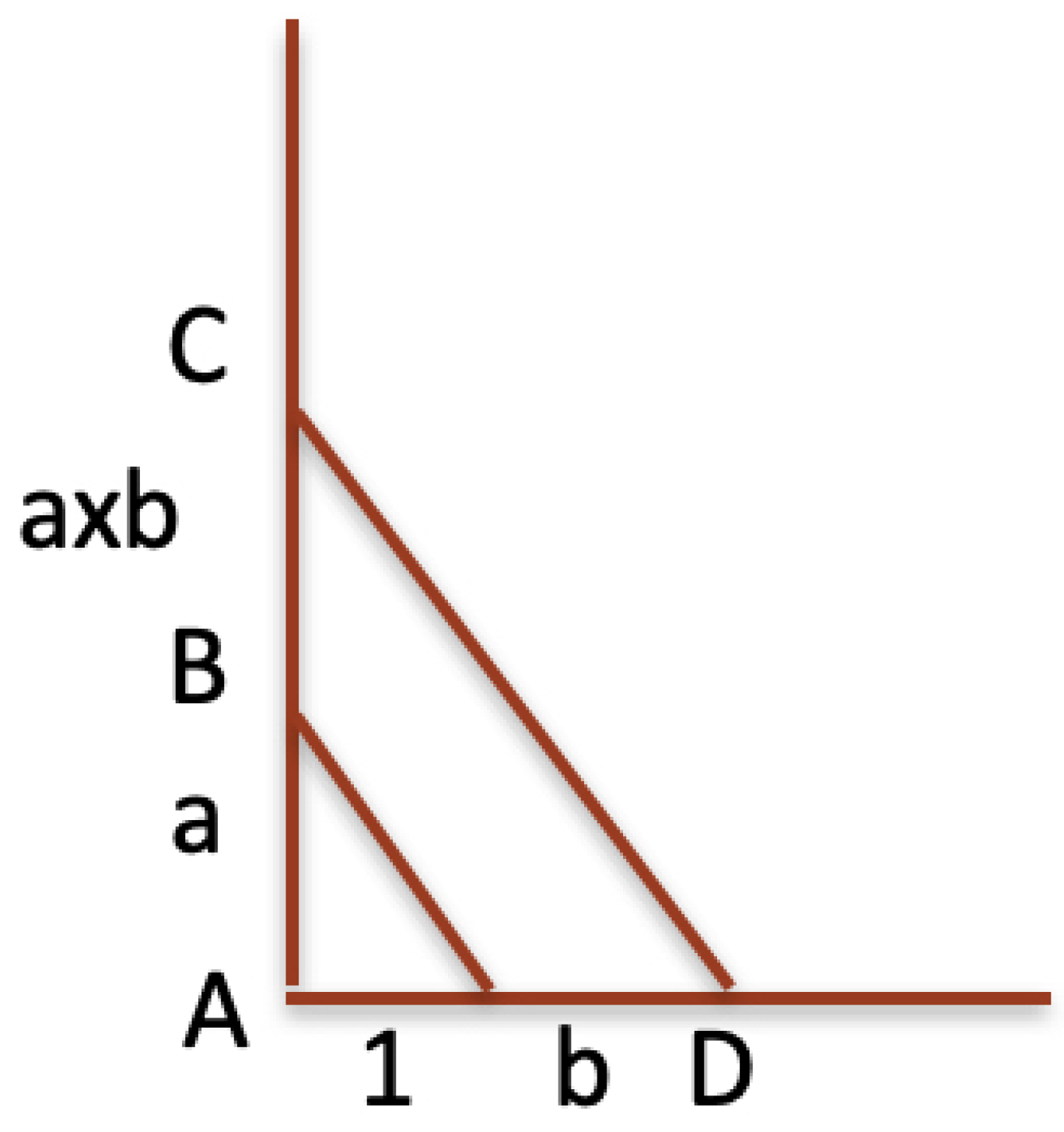
Figure 2.
The orthogonal segment multiplication (Segment has unitary length).
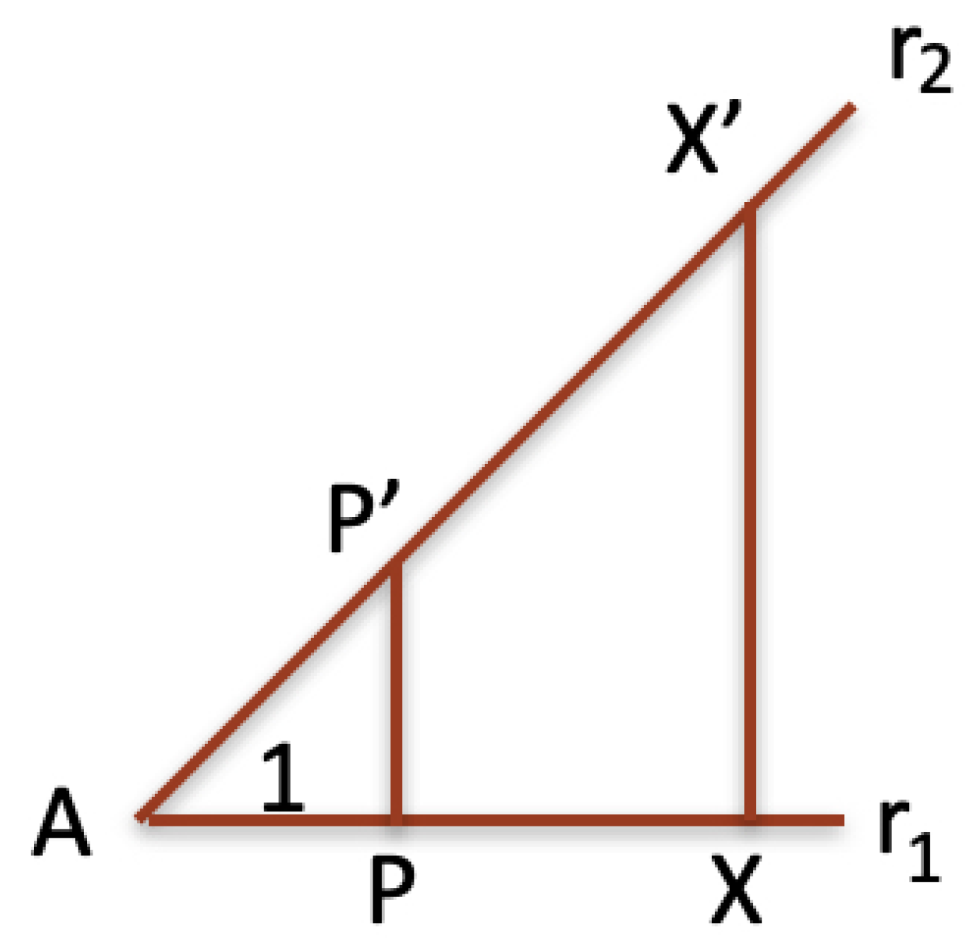
Figure 5.
Euclid’s second theorem: .
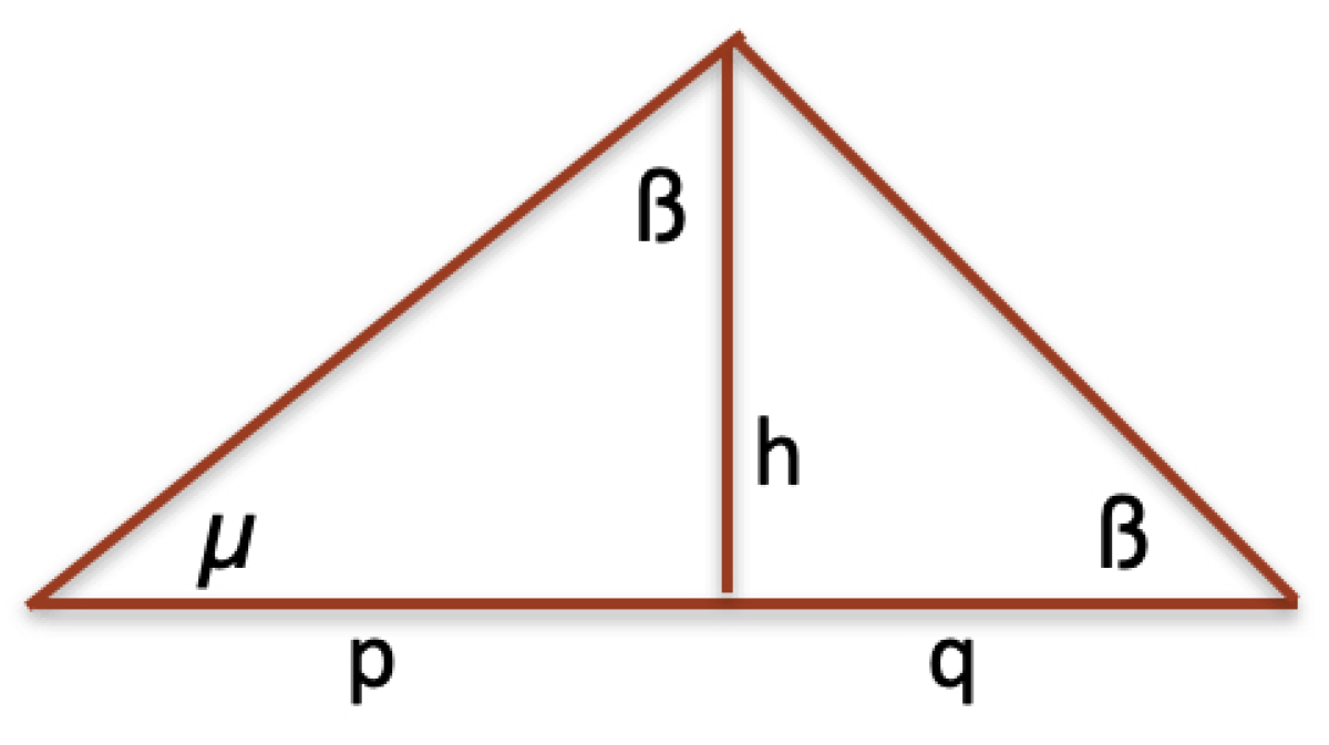
Figure 6.
The vertical segment multiplication .
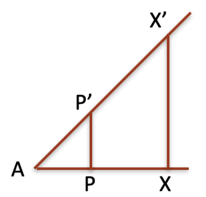
Figure 7.
The equivalence between Hilbert’s segment multiplication and vertical segment multiplication.
Figure 7.
The equivalence between Hilbert’s segment multiplication and vertical segment multiplication.
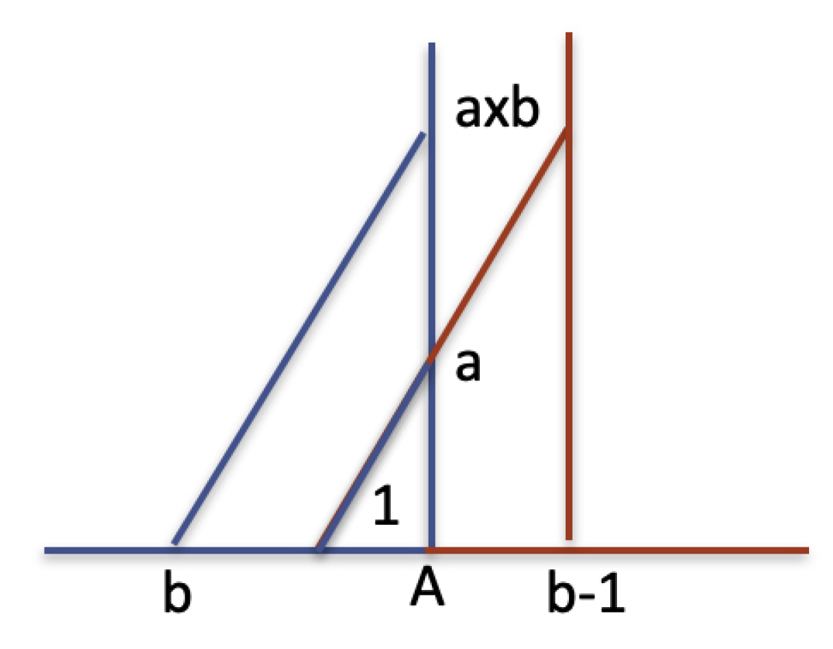
Figure 8.
If two pairs of lines are parallel, then all three pairs of lines are parallel.
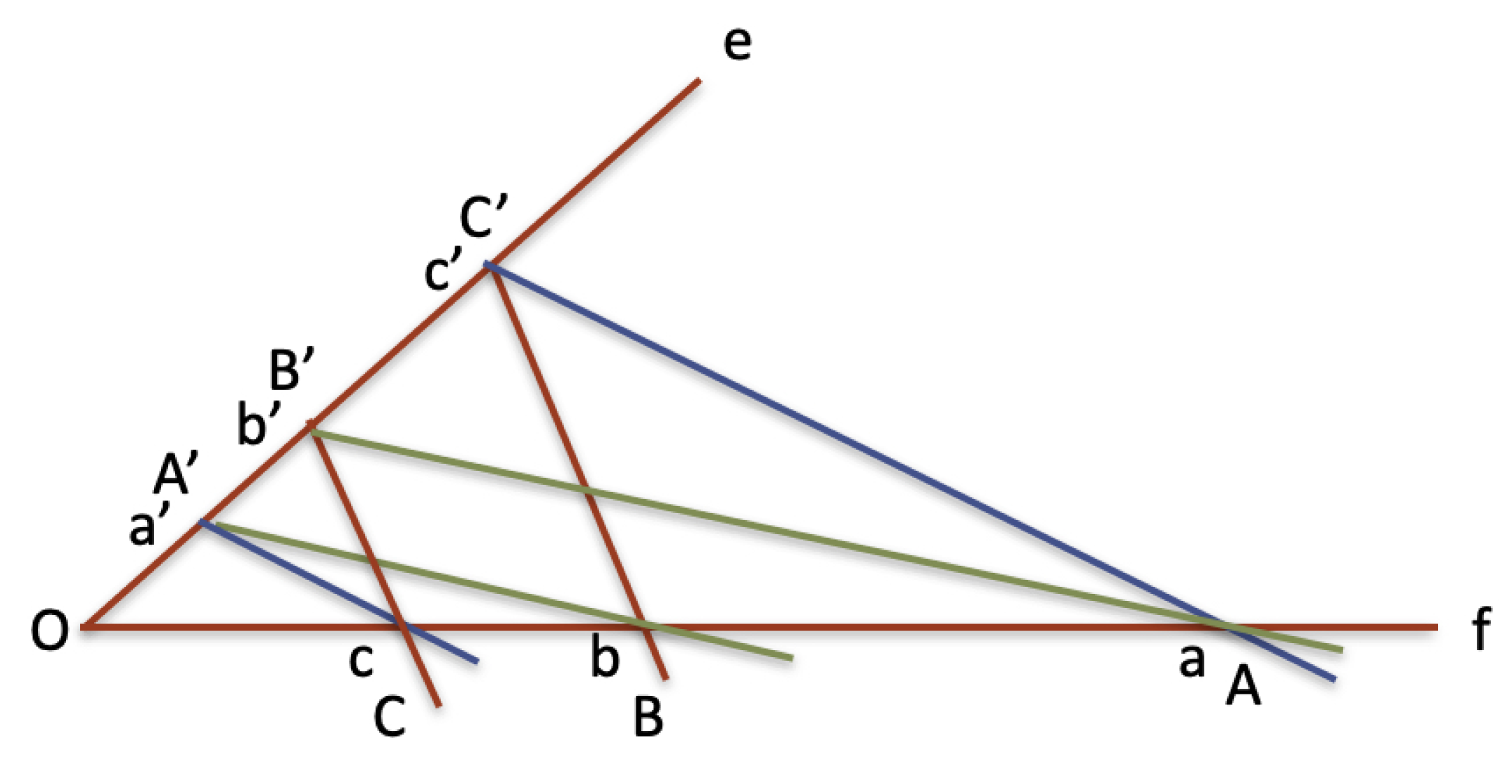
Figure 9.
The Gnomon Theorem.
Disclaimer/Publisher’s Note: The statements, opinions and data contained in all publications are solely those of the individual author(s) and contributor(s) and not of MDPI and/or the editor(s). MDPI and/or the editor(s) disclaim responsibility for any injury to people or property resulting from any ideas, methods, instructions or products referred to in the content. |
© 2025 by the author. Licensee MDPI, Basel, Switzerland. This article is an open access article distributed under the terms and conditions of the Creative Commons Attribution (CC BY) license (https://creativecommons.org/licenses/by/4.0/).
Copyright: This open access article is published under a Creative Commons CC BY 4.0 license, which permit the free download, distribution, and reuse, provided that the author and preprint are cited in any reuse.


