
Submitted:
23 September 2025
Posted:
25 September 2025
You are already at the latest version
Abstract
In high-temperature testing scenarios that rely on contact, fine-wire thermocouples demonstrate commendable dynamic performance. Nonetheless, their thermal inertia leads to notable dynamic nonlinear inaccuracies, including response delays and amplitude reduction. To mitigate these challenges, a novel dynamic error correction approach is introduced, which combines a Continuous Restricted Boltzmann Machine, Deep Belief Network, and Physics-Informed Neural Network (CDBN-PINN). The unique heat transfer properties of the thermocouple's bimetallic structure are represented through an Inverse Heat Conduction Equation (IHCP). An analysis is conducted to explore the connection between the analytical solution's ill-posed nature and the thermocouple's dynamic errors. The transient temperature response's nonlinear characteristics are captured using CRBM-DBN. To maintain physical validity and minimize noise amplification, filtered kernel regularization is applied as a constraint within the PINN framework. This approach was tested and confirmed through laser pulse calibration on thermocouples with butt-welded and ball-welded configurations of 0.25mm and 0.38mm. Findings reveal that the proposed method achieved a peak relative error of merely 0.83%, surpassing the 2.05% of the ablation technique and the 2.2% of Tikhonov regularization. In detonation tests, the corrected temperature peak reached 1045.7°C, with the relative error decreasing from 77.6% to 4.9%, and the rise time enhanced by 26 milliseconds. By merging physical constraints with data-driven methodologies, this technique successfully corrected dynamic errors even with limited sample sizes.
Keywords:
dynamic inverse filtering
; fine-wire thermocouple
; transient temperature measurement
; CRBM-DBN
; PINN
; inverse heat conduction
; error correction
1. Introduction
In scenarios involving the measurement of detonation temperature fields in artillery or warheads, as well as the combustion gas temperatures in spacecraft or automotive engines, both solid and liquid fuels, along with propellants, emit significant thermal energy rapidly during combustion. This results in the creation of transient high-temperature thermal flows, which are often accompanied by high-pressure thermal shock effects [1,2]. Accurately capturing the temperature variations within these thermal flows presents a significant challenge in the industry. Therefore, investigating transient high-temperature testing methods and associated sensors to enhance temperature measurement precision is an essential area of research.
In the realm of transient explosion temperature testing, two prevalent methods are employed: non-contact and contact temperature measurement. The non-contact approach faces challenges due to the intricate nature of fuel and agent compositions, which can result in considerable inaccuracies stemming from difficulties in measuring emissivity accurately. On the other hand, contact temperature measurement allows for direct interaction with heat flow, primarily utilizing thermocouples as the main sensing instruments. However, these thermocouples are prone to a significant time lag during dynamic testing, a phenomenon caused by the thermal inertia of their sensing components. This lag is intricately linked to the dynamic properties of the thermocouples [3,4]. When these properties fall short of engineering testing standards, the dynamic response is markedly delayed, causing the observed temperature peak to diverge from the actual value. Dynamic calibration experiments can illustrate the connection between the thermocouple’s dynamic response and the excitation source, providing a framework for assessing dynamic errors in testing [5,6]. This connection can be observed in the thermocouple’s thermal conduction effects under thermal stimulation [7] and can also be described through a dynamic mathematical model [8]. Addressing how to leverage this relationship to mitigate dynamic errors during testing is crucial for resolving this technical challenge.
Dynamic error correction represents a technique that shifts from merely optimizing data to actively rectifying errors, with its implementation viewed as a dynamic inverse operation [9,10]. This approach aims to mitigate dynamic inaccuracies stemming from the sensor’s limited dynamic properties by reversing the input values using the effective output from the thermocouple, guided by specific mathematical or physical principles [11,12]. To address the hysteresis observed in the thermocouple’s dynamic response, this correction method can be framed as an inverse heat conduction problem under defined conditions. It can be articulated as an Inverse Heat Conduction Problem (IHCP) expressed through partial differential equations, where the objective is to determine the time-dependent solution of the inverse problem within constrained boundary conditions to accurately reflect a thermal process. The challenges of this inverse problem are primarily due to its ill-posed nature, which requires careful examination before attempting a solution. Selecting a suitable regularization technique is crucial during the resolution phase [13,14].
Various algorithms have been developed for IHCP under one-dimensional geometric scenarios, including Tikhonov regularization [15] and the sequential function specification method [16]. Frankel J.I. and colleagues outlined the transient one-dimensional linear heat equation for thermocouples and introduced an optimal regularization identification technique based on the Non-Integer System Identification (NISI) method to tackle the inverse heat conduction issue [17]. J.-G. Bauzin formulated the heat transfer convolution equation using the Laplace transform and derived the correlation between boundary temperature and time through a deconvolution algorithm [18]. Farahani, S. D. and others presented an inverse heat transfer search technique [19], utilizing a K-type thermocouple as a boundary condition to determine the heat transfer coefficient of an impinging jet, while also examining how factors like measured temperature, jet velocity, and the number of thermal conductivity components influence the accuracy of the algorithm. Z.-Y. Zhou and colleagues suggested employing the Element Differential Method (EDM) in conjunction with an enhanced Levenberg-Marquardt algorithm for predicting boundary heat flux [20]. Additionally, Yu, Z. C. and others explored how the dynamic response of sensors affects surface heat flux predictions using traditional methods such as the Space Marching Method (SMM) and the Calibration Integral Equation Method (CIEM)[21], incorporating Gaussian filtering and future time regularization as their respective regularization strategies. Collectively, these investigations illustrate that when addressing inverse time-varying IHCP, integrating known thermodynamic properties, initial conditions, and boundary conditions with limited temperature data collected over time at designated points can effectively determine boundary temperature and heat flux.
Regularization techniques tackle the mathematical challenges associated with inverse problems, yet they often overlook the nonlinear aspects [22]. A prominent example of a data-driven feature extraction approach is the Deep Belief Network (DBN), which utilizes Continuous Restricted Boltzmann Machines (CRBMs) for layered feature extraction, proving effective in nonlinear environments [23,24,25]. Nevertheless, DBNs typically lack a clear physical interpretation, especially in transient high-temperature testing situations, where using thermocouples on small samples can lead to underfitting and diminished robustness.
Recent studies have begun to focus on data-driven and hybrid strategies to improve inverse modeling, seeking to resolve these challenges.In the process of solving IHCP, physics-informed neural networks (PINNs) showing exceptional efficacy in addressing transient inverse challenges, including the Navier-Stokes equations [26], Helmholtz equation [27], wave equation [28], and other related issues [29,30,31,32,33]. For instance, Fang, B. L. improved the accuracy of absorptance characterization for rough metal surfaces by aligning the temperature rise curve with a differential equation and creating a loss function using PINNs [34]. Similarly, Y. Wang and colleagues successfully determined temperature-dependent thermal conductivity by harnessing the strengths of PINNs in solving temperature fields, proving that PINNs can effectively reconstruct three-dimensional transient temperature distributions [35]. Additionally, L. Liu and associates utilized PINNs to monitor temperature variations at various points within a medium by strategically placing multiple thermocouples, leveraging PINN’s robust temperature field reconstruction capabilities alongside a novel \tracking method\ to ascertain surface heat flux and ablation sites [36].
To conclude, current techniques generally tackle the Inverse Heat Conduction Problem (IHCP) through a simplified single-layer model, failing to account for the noise amplification caused by the unstable bimetallic structure of thermocouples. While the Deep Belief Network (DBN) model is proficient in handling non-linearities, it suffers from physical inconsistencies and inefficiencies when dealing with limited data samples. The Physics-Informed Neural Network (PINN), although grounded in physical principles, struggles with time series data unless it has been pre-trained. There is a scarcity of research that has integrated regularization parameters into the PINN loss function for analyzing network errors. This study aims to resolve these challenges by introducing a new network architecture combining CRBM, DBN, and PINN, and assessing the efficacy of a dynamic inverse filtering approach for thermocouples, which incorporates regularization terms in its loss function. The proposed network is founded on the principles of thermocouple heat conduction inverse problems and employs Adam optimization to enhance the convergence speed of the CRBM-DBN. Additionally, it incorporates a spectral regularization method for the filtering kernel within the two-layer IHCP regularization framework to stabilize solutions that are ill-posed. In the PINN framework, both PDE and regularization constraints are integrated to address the shortcomings of purely data-driven methods in terms of physical accuracy.
2. Princeples and Methods
2.1. Principle of Thermocouple Dynamic Inverse Filtering
Thermocouples exhibit significant nonlinear characteristics in dynamic testing, which can be regarded as a representation of a nonlinear dynamic system. The relationship between heat flux excitation as the input and thermal response potential as the output is described using the NARMA (Nonlinear AutoRegressive Moving Average) model, as shown in the following equation:
where represents the thermoelectric potential measurement from the thermocouple at a specific time , while denotes the corresponding surface heat flux input at that same moment. The variables , , and refer to the orders of autoregression, moving average, and the delay of the input, respectively. Additionally, signifies the noise in the observations, and indicates a nonlinear function characterized by certain parameters.
Dynamic inverse filtering fundamentally involves reinterpreting the previously mentioned model as a challenge of identifying the inverse system. By employing techniques designed for addressing inverse problems, is utilized as input samples for inversion , which in turn allows for the calculation of the dynamic error.
Subsequently, utilize the inverse filtering technique to reduce . This concept is depicted in Figure 1:
2.2. Inverse Problem Analysis
The investigation into the inverse problem starts with examining the thermal transfer properties of the thermocouple. These properties indicate that a smaller junction design results in reduced thermal inertia effects. To achieve a quicker temperature response, we focus on wire-type thermocouples. This type consists of two alloy wires fused together, featuring a junction diameter in the sub-millimeter range, which allows us to disregard radial temperature variations and concentrate solely on axial heat transfer through the metal wires. The junction is identified as the point where the two wires meet, both of which are considered to be of equal length. One wire is referred to as the free end, while the other is the working end, with a boundary temperature set at 0°C, as illustrated in Figure 2:
Where represents the length of the two fine-wires that make up the thermocouple, where the working end is designated as the first layer and the free end is as the second layer, with the initial length of the working end denoted as 0. The lateral represents the boundary between the ends of the thermocouple. Define as the thermal conductivity, while indicate the thermal diffusivities for the first and second layers, respectively.
The fine-wire thermocouple features a two-layer alloy design that is uniform in length; however, when subjected to thermal stimulation at the junction, the heat transfer mechanisms of the two alloys is asymmetric, and the temperature distributions in the first and second layers are expressed by and , is the time of the heat transfer process, the subsequent partial differential equation (PDE) can be represented as follows:
where the thermal diffusivities for these layers are represented by and , the junction point is indicated by l, while 2l signifies the overall length. By incorporating the initial condition, the temperature at the starting moment (relative to the cold end) can be defined as:
The conditions at the boundaries are established based on the operational end and the unrestrained end , which can be described as:
where is the boundary temperature at the working end ;
The adiabatic boundary at the free end can be characterized as:
and interface continuity:
where represents the true heat temperature stimulation at the node, while the thermal conductivities are denoted by and .
In thermocouples, the Seebeck effect and the law of intermediate conductorsthe law governing intermediate conductors indicates that, following cold junction compensation, the temperature at the working end can be derived inversely from the actual thermoelectric potential difference produced by the thermocouple. This potential difference serves as the actual excitation response observation sample.
If we consider , and as the solution to the direct problem, it follows that, under specified conditions, both the function , and its partial derivatives reside , within the same space . By applying the known adiabatic boundary conditions at the free end, we can address the inverse problem by determining the working end’s temperature ()within the specified domain , which can be classified as a Cauchy inverse problem. The Cauchy inverse problem related to intermediate conductors is usually ill-posed, demonstrating considerable instability. Minor inaccuracies in experimental data can result in drastic variations in solutions across the interval, primarily due to the kernel function associated with the high-frequency components. To investigate this issue, a Fourier transform is applied to the two-layer domain partial differential equation, allowing it to be represented in the frequency domain as follows:
By applying the first-order partial derivative to convert it into a set of ordinary differential equations, it becomes clear that the presence of an unbounded kernel in the solution indicates that high frequencies can cause instability. In real-world experiments, the outcomes show some discrepancies, leading to the definition of the real temperature , which fulfill the following conditions:
where, the representative measurement error bound is denoted.
The ill-posedness is quantified through norm analysis, under the norm:
where, an unbounded kernel function is utilized. To ensure a stable outcome, a regularization technique involving a filtered kernel is implemented. Within the single-layer domain ( region), the unbounded kernel is substituted with a bounded filtered variant:
where denotes the regularization parameter, denotes the Sobolev order; If is a minimal value, , if , then is bounded.
The convergence theorem, which relies on the Sobolev norm, demonstrates that when the bounds of measurement error and the prior assumption —expressed as a norm within the Sobolev space — is fixed constants defined by the highest temperature range, and an appropriate regularization parameter is chosen, the subsequent convergence estimate can be derived at , the formula is as follows:
where, and represent positive constants. Given the specified conditions for and , the value of is established by .
2.3. Improved CRBM-DBN-PINN Model
This study introduces the PINN-CRBM-DBN framework to combine physical principles with data-centric methods. In this framework, CRBM-DBN is responsible for the pre-training of features, whereas PINN incorporates IHCP PDE along with regularization constraints. The framework’s design is depicted in Figure 3.
The Deep Belief Network(DBN) is a generative framework made up of several stacked layers of Restricted Boltzmann Machines(RBMs), which are utilized for identifying nonlinear systems. In this study, CRBMs are introduced to substitute the initial layer of conventional RBMs when working with thermocouple time series data, allowing for the processing of continuous inputs. The architecture of the CRBM-DBN includes a base CRBM for extracting features, along with 2-3 intermediate RBM layers for hierarchical sampling. The energy function associated with the CRBM is:
where the visible layer is denoted as (continuous input and ), while the hidden layer is indicated by a Bernoulli distribution. The parameters include weights and biases ,, along with the noise variance . The distribution conditioned on these elements is:
Traditional training employs the Contrastive Divergence (CD) algorithm to maximize the likelihood function, which is as follow:
Parameter Update is defined as follow:
where represents the latest adjustment to the weight, denotes the fundamental learning rate, signifies the anticipated interaction between visible and hidden units based on the data distribution (input data typically acquired through sampling), while reflects the expected interaction under the distribution of data reconstructed by the model. The variable stands for the momentum coefficient, which generally falls between 0.5 and 0.9, and is utilized to enhance training speed and minimize fluctuations. Additionally, indicates the weight adjustment from the preceding time step, serving as the momentum component.
The Adam optimizer was developed to supersede the constant learning rate of CD, improving convergence for dynamic sequences. It employs both momentum and adaptive learning rates:
where represents the adaptive learning rate at the time step , substituting in the fundamental iterative equation, while denotes the base learning rate, is the decay rate for the first moment estimate, commonly set at 0.9, is the decay rate for the second moment estimate, usually set at 0.999, and refers to the first moment estimate of the weight gradient, which is computed using the following formula:
where represents the present gradient, while denotes the approximation of the second moment (uncentered variance) related to the weight gradient, with the following formula for computation:
To ensure stability during training, the learning rate adjustment factor is limited to , avoiding issues that may arise from learning rates that are too high or too low. The output generated from the forward pre-training of the enhanced CRBM-DBN serves as the input for the PINN, which is designed to create an error assessment framework. This framework consists of two evaluation phases: the training phase, which concentrates on convergence and optimization, and the overall model assessment, which highlights time-domain features and robustness. The goal is to measure the accuracy, interpretability, generalization ability, and practical application of the framework.
The total loss function of PINN is defined as:
where the data residual can be characterized as:
where represents the count of training examples. This formula indicates the total loss experienced by the data layer following the training of DBN. The physical residuals associated with the two-layer PDE can be described as:
The filtering-kernel regularization specifically targets IHCP’s high-frequency ill-posedness by applying a spectral filter in the loss function:
where the filtering kernel reduces high-frequency noise, and its sensitivity to noise is influenced by the regularization parameter .
The overall training procedure for the network is outlined as follows:
1.CRBM-DBN Initial Training: Employ laser pulse data to derive time-domain features using Adam optimization for initializing the weights of the PINN;
2. PINN Adjustment: Incorporate two layers of IHCP PDE constraints and refine hyperparameters via Bayesian optimization;
3. Solving Inverse Problems: The network generates the best solution , assessed through metrics like peak value and time constant, along with cross-validation and normalized mean square error (NMSE).
3. Experiment
3.1. Laser Narrow Pulse Calibration Platform
A calibration platform featuring a laser pulse was developed to capture the transient thermal behavior of the thermocouple. This setup allows the thermocouple to replicate the rapid thermal changes caused by explosive thermal shock by detecting the brief surface temperature changes induced by the laser. The platform’s design includes a powerful laser source, a system for beam uniformity, and a digital system for signal collection and analysis. The block diagram of the system is illustrated in Figure 4, and Figure 5 presents the actual design of the calibration platform.
The laser system utilizes a powerful laser sourced from Raycus. A pulsed laser control mechanism is implemented to toggle the laser on and off, allowing for the creation of a variable pulsed laser. Due to the non-stationary nature of the laser spectrum, a beam homogenization setup was developed, featuring a microlens array that segments and recombines the laser beam. This modulation technique evens out the power density of the laser spot, boosts efficiency, and enhances the precision of the calibration platform. A calibrated thermocouple is mounted on a bracket, and the laser, after passing through the homogenization setup, heats the junction’s surface. At the same time, the probe of a high-speed infrared thermometer is positioned in line with the calibrated thermocouple. The thermocouple’s response signal is processed through a conditioning circuit and, along with the infrared thermometer’s signal, is gathered and recorded by the NI-6115 data acquisition system. The host computer then carries out digital cold junction compensation and data analysis.
The calibration platform for laser narrow pulses employs the IGA 740-LO high-speed infrared thermometer, which has a temperature range from 300 to 2300°C. This necessitates adjustments for readings in the lower temperature range. The infrared thermometer’s probe can measure diameters smaller than 0.1mm and boasts a response time of 6μs, allowing it to closely match the laser excitation at the thermocouple junction’s surface. Therefore, the temperature readings obtained from the infrared thermometer are considered to accurately reflect the surface temperature of the thermocouple junction.
Prior to its application, the surface emissivity of the thermocouple must be configured. To accurately determine this emissivity in a lab environment, the Modline 5 pyrometer from IRCON was utilized to assess the actual surface temperature of the test object. Initially, the thermocouple was heated with a low-power laser until it achieved thermal equilibrium, at which point the surface temperature of the thermocouple junction was recorded using both the pyrometer and the infrared thermometer. The temperature output from the pyrometer was noted, and adjustments to the infrared thermometer’s emissivity were made until the readings from both devices aligned. The emissivity value established on the infrared thermometer at this stage was then regarded as the surface emissivity of the thermocouple junction, which was found to be approximately 0.4 during this experiment.
3.2. Experimental Steps
The developed platform for laser dynamic calibration was employed to create pulse excitation signals. The output power of the laser pulse generator was modified in percentage increments, specifically set to 80%, 90%, and 100% of its peak capacity through the host computer. At full power, the theoretical maximum temperature remains below 1000°C. The duration of the laser emission was regulated by a square wave with an equal duty cycle produced by the pulse signal generator, with the emission duration established at 5ms to replicate transient thermal events. The subjects of the tests included OMEGA’s butt-welded and ball-welded thermocouple, featuring diameters of 0.25mm and 0.38mm, respectively, made from type K nickel-chromium/nickel-silicon alloy. The configuration of the thermocouple junction is illustrated in Figure 6.
The data obtained from the infrared thermometer under identical conditions were analyzed. As previously noted, readings taken by the infrared thermometer in cooler temperatures necessitate adjustments. Utilizing the heat conduction differential equation along with the boundary conditions for laser heating of solid metals, the temperature at the metal’s surface can be expressed as:
where represents the duration of the laser pulse, denotes the density of laser power, and indicates the absorptivity of the metal. By applying the formula for the laser heating duration found in Equation (24), we analyzed the temperature variation within the range of 0-300°C. Additionally, we recorded the temperature increase beyond 300°C using an infrared thermometer. Figure 7 illustrates the results obtained from thermocouples attached to 0.25mm diameter butt welds, tested at power levels between 80% and 100%. Given that the testing conditions remained constant and a digital temperature compensation technique was employed by the host computer, we adjusted the baseline of the two distinct response outcomes for uniformity, aligning their starting temperatures with the laboratory’s ambient temperature of 22.3°C.
Figure 7 clearly illustrates that the infrared thermometer has a quicker rise time than the thermocouple, with a more significant difference in amplitude. The thermocouples’ response shows a distinct delay, and the temperature peak variations across the three data sets fall between 300-500°C. Furthermore, while increased power leads to higher temperatures for the thermocouple, the time constant remains relatively stable. Consequently, a uniform laser pulse excitation at 100% power was employed in the following experiments. This study also examines how fine-wire diameter and junction design affect the dynamic response of thermocouples. Under 100% power laser narrow pulse excitation, 20 repeated tests were performed on K-type ball-welded and butt-welded thermocouple with diameters of 0.25mm and 0.38mm, respectively, to create a dynamic response sample set. The thermocouple junction was cleaned every 5 experiments to minimize the effects of the oxide layer. The individual experimental outcomes of junctions with varying junction designs at fine-wire diameters of 0.25mm and 0.38mm were compared, with the findings displayed in Figure 8.
The butt-welded thermocouple demonstrates a notably quicker rise time than the ball-welded thermocouple, allowing it to detect higher peak temperatures more effectively. Nevertheless, an increase in fine-wire diameter results in a reduction of both rise time and peak temperature, suggesting that the butt-welded thermocouple has a lower heat capacity and responds more rapidly at equivalent diameters. This indicates that when subjected to the same transient thermal shock, the two types of thermocouples will show varying dynamic errors, with the ball-welded version suffering from greater lag and reduced amplitude.
4. Results and Analysis
4.1. Model Accuracy Analysis
In the context of establishing a specific laser excitation and utilizing a thermocouple with a fine-wire diameter of 0.25mm, the analysis focuses on the effectiveness of a dynamic error correction model for thermocouples featuring various junction configurations. To enhance network training efficiency, 500 valid signal points are selected from 20 measured samples, creating a new sample set that is evenly split into training and testing subsets. The input data for the network undergoes normalization, and the original temperature readings are retrieved using the temperature-electromotive force table. The network’s batch size is determined to be 100 based on the dataset length, with each layer containing 20 neurons. Initially, to assess the network’s performance and avoid reverse convergence, the iteration count is set to 250, with the loss function’s initial weights established at , =0.1 and =0.1. Given the considerable errors encountered during transient high-temperature assessments, the measurement error threshold is defined as 1% of the thermocouple’s full scale, equating to 1, which leads to a regularization parameter of 0.032. The laser pulse excitation signals, captured by the corresponding infrared thermometer, serve as the target sample set. The normalized minimum mean square error (NMSE) between the network’s output and the training samples is employed as the evaluation metric. The variations in the first term of the RBM layer’s network weights and the hidden layer feature values throughout the training process, both before and after the integration of PINN, were documented for a set of training samples, as illustrated in Figure 8(a) and (b).
In Figure 8(a), the weights and eigenvalues display considerable variability, indicating that the entirely data-driven CRBM-DBN is vulnerable to noise during the initial gradient updates, which causes instability in the parameters. By the 90th iteration, the weights and eigenvalues of the hidden layer begin to stabilize, yet the eigenvalues still experience slight fluctuations, suggesting that while the network has started to recognize data patterns, it lacks physical constraints, leading to persistent oscillations. In contrast, Figure 8(b) shows that despite a larger initial fluctuation range, the system can rapidly stabilize within a manageable range due to the IHCP PDE constraints and filter kernel regularization implemented by PINN, which mitigates high-frequency noise. Following fine-tuning with PINN, convergence is reached around the 120th iteration, accompanied by reduced eigenvalue fluctuations, with h1, h2, and h3 appearing nearly smooth. This supports the notion that incorporating physical priors enhances the resolution of inverse problems in PINN during data-driven pretraining. Furthermore, after over 250 iterations, the network weights for RBM1, RBM2, and CRBM layers in Figure 8(a) near the 90th iteration, along with the hidden layer eigenvalues, show signs of convergence, albeit with minor fluctuations still evident. In Figure 8(b), the weights and eigenvalues demonstrate manageable fluctuations in the early iteration phases, and post fine-tuning with PINN, they achieve convergence around the 120th iteration with even lesser eigenvalue fluctuations, confirming the success of the entire forward training and reverse fine-tuning methodology. Additionally, the impact of Adam optimization has been validated, as illustrated in Figure 9.
In Figure 9, both approaches demonstrate a swift decrease during the initial iterations, indicative of Adam’s adaptive learning rate and momentum strategy, which enhance early gradient updates and rapidly identify data trends. The CRBM-DBN-PINN model reaches convergence at approximately 1e-4 after around 120 iterations, surpassing the ablation PINN that stabilizes at roughly 1e-3. The use of Adam optimization facilitates faster convergence, while the addition of PINN’s physical constraints raises computational demands, resulting in a greater number of iterations needed for convergence but yielding improved accuracy. This illustrates the effectiveness of the Adam algorithm in optimizing networks and underscores the enhanced accuracy benefits of PINN throughout the convergence phase.
Subsequently, we will evaluate the network’s performance. Regarding the loss function, in addition to determining weight values and , must also be addressed the choice of regularization parameter . We will first assess the optimal regularization parameter by testing various values while maintaining other conditions constant. To ensure a meaningful effect of , we set , and to 1, 3, and 7 for training samples, followed by validation with the test set. The outcomes of the 0.25mm butt welding and the ball-welded thermocouple before and after adjustment are illustrated in Figure 10(a) and (b):
The statistical analysis of the key feature data presented in the Figure 10 is conducted, and the relative error is computed, with the findings shown in Table 1.
Figure 10(a) illustrates that the correction curves for the ball-welded thermocouple across three different p values closely align with the standard curve. The correction curve for p=1 is similar to the infrared measurement but falls short at the peak; the p=3 correction shows a higher peak, while p=7 proves to be the most effective, nearly matching the standard value with minimal delay. This indicates that increasing the p value improves regularization and reduces high-frequency noise. Similarly, Figure 10(b) exhibits the same trend as Figure 10(a), highlighting the most accurate approximation and the peak nearest to the standard value at p=7.
The findings demonstrate that the spectral regularization technique effectively addresses dynamic inaccuracies in both thermocouple types, with the parameter p playing a crucial role. It is recommended to opt for a higher value of p during selection. Furthermore, to enhance the precision of convergence, the weight assigned to the regularization term should be lower than that of the other two components in the Loss function, thereby reducing the regularization parameter’s effect on the overall assessment framework. The suggested ranges for the hyperparameters are [0.8,1.0], [0.1,0.2] and [0.01,0.05]. Optimal weights are determined adaptively through Bayesian optimization throughout the training phase. 3-fold cross-validation approach was utilized, allocating 70% of the data for training and 30% for testing. The actual samples were split into two categories for comparative analysis to assess the effectiveness of dynamic error correction: 1.a comparison of 0.25mm and 0.38mm ball-welded thermocouples, 2.a comparison of 0.25mm and 0.38mm butt-welded thermocouples. The NMSE criterion was established as the evaluation standard during the training phase.
where represents the value predicted by the network, while denotes the real measurement obtained from the infrared thermometer, and signifies the total number of samples. The criterion established is NMSE < 0.01, which reflects effective convergence, indicating that the process continues until the lowest convergence value is achieved. To avoid overfitting, an early stopping criterion is implemented based on the increase of NMSE in the test dataset. The statistical analysis of the test sample results, both pre- and post-correction, is illustrated in Figure 11 (a) and (b).
In Figure 11(a), the correction curves for various fine-wire diameters closely align with the standard curve, exhibiting a notable enhancement in rise time. The peak temperature is nearly equivalent to the standard value, though there is a slight deviation in the peak location, with the 0.25mm diameter showing better performance than the 0.38mm. Figure 11(b) illustrates that the correction curve for the butt-weld thermocouple also closely matches the standard, with improved rise time, and again, the 0.25mm diameter outperforms the 0.38mm. The key difference is the more consistent peak temperature points when compared to the ball-welded thermocouple, leading to an overall superior approximation effect, which can be attributed to its junction design that facilitates quicker response times and higher temperatures. We have conducted a statistical analysis of all test samples, as detailed in Table 2.
Analysis of Table 2 indicates that the butt-welded junction outperforms the ball welded junction, as evidenced by its lower RE and higher R2 values. This superior performance is attributed to its reduced heat capacity and quicker response time. Additionally, a thermocouple featuring a finer wire diameter of 0.25mm demonstrates enhanced performance compared to one with a thicker 0.38mm fine-wire, although the temperature peaks show only minor variations. The rise time for the modified ball-welded has seen a notable enhancement, nearly matching the improvements observed in the butt-welded design, thus confirming the efficacy of the proposed approach for thermocouples with varying junction configurations and fine-wire sizes. To further assess the algorithm’s effectiveness, we focused on the 0.25mm butt-welded thermocouple and compared the dynamic error correction outcomes of our method against those of the conventional regularization technique and the ablation method, as illustrated in Figure 12.
Figure 12 illustrates that all three approaches approximate the standard curve, but the conventional Tikhonov method demonstrates a less accurate fit, characterized by significant fluctuations. The temperature peak surpasses the standard value, and there is a considerable shift in the peak position. The ablation technique shows marked enhancement compared to the traditional approach, yet it still presents some fluctuations, with its temperature peak falling short of the proposed CRBM-DBN-PINN method. Table 3 presents the quantitative correction indices before and after the adjustments.
Table 2 illustrates that the suggested approach reaches an R2 value of 0.948 for the 0.25mm butt-welded thermocouple, exhibiting a maximum relative error of merely 3.2%. This result greatly surpasses the performance of conventional Tikhonov methods and the solely data-driven CRBM-DBN-BP techniques. This clearly highlights the advantages of combining physical principles with data-driven methods for correcting dynamic errors.
4.2. Blast Test and Result Analysis
In order to acquire a detailed transient temperature distribution during the explosion test, a method involving distributed measurements is commonly utilized. A cloud explosive agent equivalent to 5kg of TNT is deployed, and an infrared thermal imager captures the fireball’s extent within a circular area of 6 meters in radius. Given the constraints of K-type thermocouples for temperature readings, two thermocouples, each with a fine-wire diameter of 0.25mm and featuring two junction structures, are secured in protective tubes and positioned at ground level near the fireball’s perimeter (6 meters from the explosive source and 40 centimeters high). The testing system logs the resulting data curves, as illustrated in Figure 13.
The proposed framework is utilized to analyze the data, yielding the results for dynamic error correction, illustrated in Figure 14.
In Figure 14, the initial curve for the butt-welded thermocouple shows a much steeper ascent compared to the ball-welded thermocouple; however, its maximum temperature is lower than that of the ball-welded. Additionally, there are significant variations during the ascent, which could be linked to the secondary combustion properties of the cloud explosive material. Following adjustments, the temperature peaks for both thermocouples have risen considerably, with the butt-welded thermocouple achieving a peak that surpasses that of the ball-welded one. Conversely, the ball-welded thermocouple has experienced a more pronounced improvement in its rise time, resulting in a closer alignment between the two after correction. The theoretical analysis of the explosive agent suggests that the temperature peak at the 6m perimeter of the fireball is projected to reach 1100℃. We also made statistics on the eigenvalues of the results, and the results are shown in Table 4:
Table 4 indicates a notable increase in the temperature peaks of thermocouples featuring both junction designs. The corrected temperature peak for the butt-welded structure demonstrates better performance, whereas the ball-welded shows a more significant enhancement in rise time. Following comprehensive adjustments, the consistency of the results aligns more closely with those achieved in a controlled laboratory setting. Nevertheless, factors such as the thermocouple’s protective casing, the detonation environment, and other variables contribute to a remaining discrepancy between the corrected outcomes and the theoretical predictions [38]. Still, the temperature peak has seen substantial improvement, nearing the actual temperature values.
5. Discussions
The peak temperature and the time it takes to reach that peak are crucial indicators of a thermocouple’s dynamic behavior. The proposed calibration method for laser pulse samples resulted in a 9.5% increase in R2, a reduction in peak error of about 1.4%, and an enhancement of rise time by more than 31ms. This suggests that the new approach markedly outperforms traditional techniques like Tikhonov and the purely data-driven CRBM-DBN-BP in terms of temperature peak and rise time. It highlights the importance of thermal conduction physics-informed constraints introduced by PINN in optimizing the performance of networks when addressing the asymmetric IHCP for thermocouple bimetallic structures. By incorporating PDE constraints, the method not only boosts accuracy but also strengthens resilience against noise, avoiding solutions that breach physical principles, unlike the purely data-driven DBN network [25,39]. The CRBM-DBN’s pre-training mechanism effectively captures nonlinear temporal features from transient responses, yielding reliable predictions for future solutions while reducing the influence of data residuals on the PINN loss function [24]. This pre-trained model is also adept at identifying predictive features across various time series. We integrated a filtering kernel regularization constraint into the PINN loss function, which, in contrast to conventional Tikhonov regularization methods [15,17], proves to be more effective in mitigating noise amplification and achieving notable dynamic error correction in small sample detonation tests. This methodology offers valuable insights for other transient tests involving limited samples. While this approach focuses on dynamic error correction for filamentary thermocouples, it can also be adapted for other fast-response thermocouple sensors or nonlinear materials with delayed temperature responses by modifying the loss function weights [34,35,36].
Despite the advancements, this framework has its drawbacks. Firstly, while the filtering kernel helps reduce ill-posedness, the non-uniqueness of solutions in high-dimensional scenarios (like three-dimensional thermocouple arrays) may result in greater errors [12]. Additionally, PINN faces convergence challenges under discontinuous boundary conditions, necessitating further hyperparameter tuning [33]. The generative pre-training of CRBM-DBN is susceptible to overfitting, particularly with sparse data, which could undermine physical consistency [39]. Overall, these challenges arise from the intricacies of multidimensional IHCP and the opaque nature of deep learning, yet the applicability of this method can be broadened by integrating PCA techniques with feature sensitivity analysis.
6. Conclusions
This study focuses on the challenge of dynamic inaccuracies in transient high-temperature readings due to the limited dynamic properties of thermocouples. We reformulated the correction of dynamic errors in thermocouples as an inverse heat conduction issue, introducing and validating a hybrid model that combines CRBM-DBN with PINN to tackle this inverse problem. A novel aspect of our approach is the incorporation of a filtering kernel regularization constraint within the PINN loss function, aimed at improving the convergence of errors. Experimental findings reveal that, as theoretically anticipated, the butt-welded and spherical-welded thermocouples exhibit distinct dynamic properties, with the butt-welded junction demonstrating a faster inherent response due to its lower heat capacity compared to the spherical-welded junction. For the same wire diameter, the original response signal from the spherical weld thermocouple shows greater time lag and amplitude reduction. The CRBM-DBN-PINN network effectively mitigates the dynamic errors in both types of sensors, achieving a relative temperature reconstruction error of less than 1% and under 5% in laser calibration and detonation tests, respectively, significantly surpassing conventional techniques. This approach is not only suitable for fine-wire thermocouples but also shows a degree of applicability for sensors exhibiting similar thermal hysteresis. This research not only delivers a precise method for correcting dynamic errors in thermocouples but also establishes a valuable research framework that integrates physical mechanisms with data-driven strategies for solving dynamic inverse problems in various sensor types. Future investigations could further explore the connections between model parameters and physical characteristics, such as junction design and heat capacity.
Author Contributions
Conceptualization, C.Z. and J.Z.; methodology, C.Z.; software, G.Z.; validation, C.Z., J.Z. and G.Z.; formal analysis, G.Z.; investigation, J.Z.; resources, J.Z.; data curation, C.Z.; writing—original draft preparation, C.Z.; writing—review and editing, G.Z.; supervision, J.Z.; project administration, C.Z. and J.Z.; funding acquisition, C.Z.. All authors have read and agreed to the published version of the manuscript.
Funding
This research was funded in part by the Natural Science Foundation of Shanxi Province under grant number 202203021222285 and in part by the Natural Science Foundation of Shanxi Province under grant number 202403021211087.
Conflicts of Interest
The authors declare no conflicts of interest.
References
- Li, Z. L., Wang, G., Yin, J. P., Xue, H. X., Guo, J. Q., Wang, Y., Huang, M. G. Development and Performance Analysis of an Atomic Layer Thermopile Sensor for Composite Heat Flux Testing in an Explosive Environment. Electronics 2023, 12(17), 18, 3582. [CrossRef]
- Cardillo, D., Battista, F., Gallo, G., Mungiguerra, S., Savino, R. Experimental Firing Test Campaign and Nozzle Heat Transfer Reconstruction in a 200 N Hybrid Rocket Engine with Different Paraffin-Based Fuel Grain Lengths. Aerospace 2023, 10(6), 20, 546. [CrossRef]
- Liu, S. Y., Huang, Y., He, Y., Zhu, Y. Q., Wang, Z. H. Review of Development and Comparison of Surface Thermometry Methods in Combustion Environments: Principles, Current State of the Art, and Applications [Review]. Processes 2022, 10(12), 40, 2528. [CrossRef]
- Tomczyk, K., Benko, P. Analysis of the Upper Bound of Dynamic Error Obtained during Temperature Measurements. Energies 2022, 15(19), 13, 7300. [CrossRef]
- Xu, S. Y., Wang, Z. H., Gui, L. J. Contact mode thermal sensors for ultrahigh-temperature region of 2000–3500k. Rare Metals 2019, (8). [CrossRef]
- Wang, F. X., Lin, Z. Y., Zhang, Z. J., Li, Y. F., Chen, H. Z., Liu, J. Q., Li, C. Fabrication and Calibration of Pt-Rh10/Pt Thin-Film Thermocouple. Micromachines 2023, 14(1), 15, 4. [CrossRef]
- Kou, Z. H., Wu, R. X., Wang, Q. Y., Li, B. B., Li, C. Z., & Yin, X. Y. Heat transfer error analysis of high-temperature wall temperature measurement using thermocouple. Case Studies in Thermal Engineering 2024, 59, 13, Article 104518. [CrossRef]
- Jaremkiewicz, M.. Reduction of dynamic error in measurements of transient fluid temperature. Archives of Thermodynamics 2011, 32(4), 55-66. [CrossRef]
- Yang, Z. X., Meng, X. F. Study on transient temperature generator and dynamic compensation technology. Applied Mechanics & Materials 2014, 511-512, 161-164. [CrossRef]
- Liu, S. Y., Huang, Y., He, Y., Zhu, Y. Q., Wang, Z. H. Review of Development and Comparison of Surface Thermometry Methods in Combustion Environments: Principles, Current State of the Art, and Applications [Review]. Processes 2022, 10(12), 40, Article 2528. [CrossRef]
- Guo, Y. K., Zhang, Z. J., Li, Y. F., Wang, W. Z. C-type two-thermocouple sensor design between 1000 and 1700 °C. Review of Scientific Instruments 2024, 95(10), 12, 105119. [CrossRef]
- Chu, J. R., Wang, S. L., Gan, R. L., Wang, W. H., Li, B. R., Yang, G. Dynamic compensation by coupled triple-thermocouples for temperature measurement error of high-temperature gas flow. Transactions of the Institute of Measurement and Control 2024, 46(5), 952-961. [CrossRef]
- Woolley, J. W., Woodbury, K. A. Thermocouple Data in the Inverse Heat Conduction Problem. Heat Transfer Engineering 2011, 32(9), 811-825. [CrossRef]
- Chen, Y. Y., Frankel, J. I., Keyhani, M. Nonlinear, rescaling-based inverse heat conduction calibration method and optimal regularization parameter strategy. Journal of Thermophysics and Heat Transfer 2016, 30(1), 67-88. [CrossRef]
- Samadi, F., Woodbury, K., Kowsary, F. Optimal combinations of tikhonov regularization orders for ihcps. International Journal of Thermal Sciences, 2021, 161(000), 106697. [CrossRef]
- Wang, F., Zhang, P., Wang, Y., Sun, C., & Xia, X. Real-time identification of severe heat loads over external interface of lightweight thermal protection system. Thermal science and engineering progress 2023, 37. [CrossRef]
- Frankel, J. I., Chen, H.. Analytical developments and experimental validation of a thermocouple model through an experimentally acquired impulse response function. International Journal of Heat and Mass Transfer 2019, 141, 1301-1314. [CrossRef]
- J.-G. Bauzin, M.-B. Cherikh, N. Laraqi, Identification of thermal boundary conditions and the thermal expansion coefficient of a solid from deformation measurements, Int. J. Therm. Sci. 2021, 164, 106868. [CrossRef]
- Farahani, S. D., Kisomi, M. S. Experimental estimation of temperature-dependent thermal conductivity coefficient by using inverse method and remote boundary condition. International Communications in Heat and Mass Transfer 2020, 117, 104736. [CrossRef]
- Z.-Y. Zhou, B. Ruan, et al. A new method to identify non-steady thermal load based on element differential method, Int. J. Heat Mass Transf. 2023, 213, 124352. [CrossRef]
- Yu, Z. C., Chen, H. C., Qi, L., Wu, Z. Calibration Method for Inverse Heat Conduction Problems Under Sensor Delay and Attenuation. Journal of Thermophysics and Heat Transfer 2025, 39(3), 595-606. [CrossRef]
- Gautam, A., Zafar, S. Ann based direct modelling of t type thermocouple for alleviating non linearity. Communications in Computer and Information Science2020, 1229. [CrossRef]
- Qiao, J., Wang, L. Nonlinear system modeling and application based on restricted Boltzmann machine and improved BP neural network. Appl Intell 2021, 51, 37–50. [CrossRef]
- Dai, H., Shang, S. P., Lei, F. M., Liu, K., Zhang, X. N., Wei, G. M., Xie, Y. S., Yang, S., Lin, R., Zhang, W. J. CRBM-DBN-based prediction effects inter-comparison for significant wave height with different patterns. Ocean Engineering 2021, 236, 10, 109559. [CrossRef]
- F. TIAN, C. YANG. Deep belief network-hidden markov model based nonlinear equalizer for vcsel based optical interconnect. Science China(Information Sciences) 2020, 63(06), 155-163. [CrossRef]
- G. Wang, Z. Chen, H. Chen, Z. Mao. Spatiotemporal-response-correlation-based model predictive control of heat conduction temperature field, J. Process Control 2024, 140, 103257. [CrossRef]
- S. Basir, I. Senocak, Physics and equality constrained artificial neural networks: application to forward and inverse problems with multi-fidelity data fusion, J. Comput. Phys. 2022, 463, 111301. [CrossRef]
- B. Moseley, A. Markham, T. Nissen-Meyer. Finite basis physics-informed neural networks(FBPINNs): a scalable domain decomposition approach for solving differential equations, Adv. Comput. Math. 2023, 49(4), 62. [CrossRef]
- H. Son, S.W. Cho, H.J. Hwang, (2023). Enhanced physics-informed neural networks with augmented Lagrangian relaxation method (AL-PINNs), Neurocomputing 548, 126424. [CrossRef]
- J. Bai, G.-R. Liu, A. Gupta, L. Alzubaidi, X.-Q. Feng, Y. Gu. Physics-informed radial basis network (PIRBN): a local approximating neural network for solving nonlinear partial differential equations, Comput. Methods Appl. Mech. Eng. 2023, 415, 116290. [CrossRef]
- F. Sahli Costabal, S. Pezzuto, P. Perdikaris. Δ -PINNs: physics-informed neural networks on complex geometries, Eng. Appl. Artif. Intell. 2024, 127, 107324. [CrossRef]
- X. Jiang, X. Wang, Z. Wen, E. Li, H. Wang, Practical uncertainty quantification for space-dependent inverse heat conduction problem via ensemble physics-informed neural networks, Int. Commun. Heat Mass Transf. 2023, 147, 106940. [CrossRef]
- K.-Q. Li, Z.-Y. Yin, N. Zhang, J. Li. A PINN-based modelling approach for hydromechanical behaviour of unsaturated expansive soils. Comput. Geotech. 2024, 169, 106174. [CrossRef]
- Fang, B. L., Wu, J. J., Wang, S., Wu, Z. J., Li, T. Z., Zhang, Y., Yang, P. L., & Wang, J. G. Measurement method of metal surface absorptivity based on physics-informed neural network. Acta Physica Sinica 2024, 73(9), 8, 094301. [CrossRef]
- Y. Wang, Q. Ren. A versatile inversion approach for space/temperature/time related thermal conductivity via deep learning, Int. J. Heat Mass Transf. 2022, 186, 122444. [CrossRef]
- Liu, L., Liang, Y., Shang, Y. B., & Liu, D. H. Identification of ablation surface evolution using physics-informed neural network. International Communications in Heat and Mass Transfer 2025, 167, 13, 109310. [CrossRef]
- Zhao, C., & Zhang, Z. Dynamic error correction of filament thermocouples with different structures of junction based on inverse filtering method. Micromachines 2020, 11(1). [CrossRef]
- Sun, J. Z., Liu, B. D., Xu, P. C., & Wang, P. Y. Influence of protection tube on thermocouple effect length. Case Studies in Thermal Engineering 2021, 26, 11, 101178. [CrossRef]
- Zhao, C., & Zhang, Z. Inverse filtering method of bare thermocouple for transient high-temperature test with improved deep belief network. IEEE Access 2021, PP(99). [CrossRef]
Figure 1.
Dynamic filter principle.
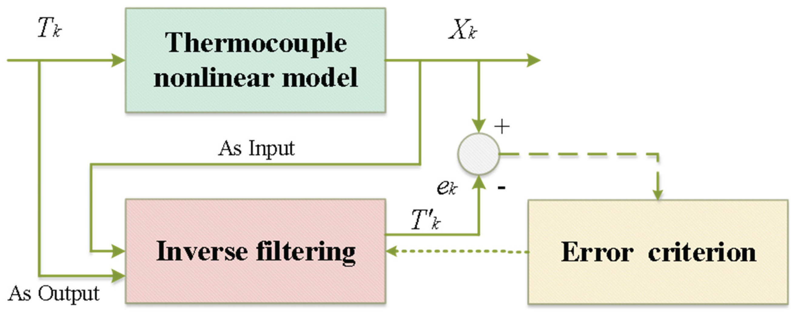
Figure 2.
Two-layer domain structure of thermocouple.
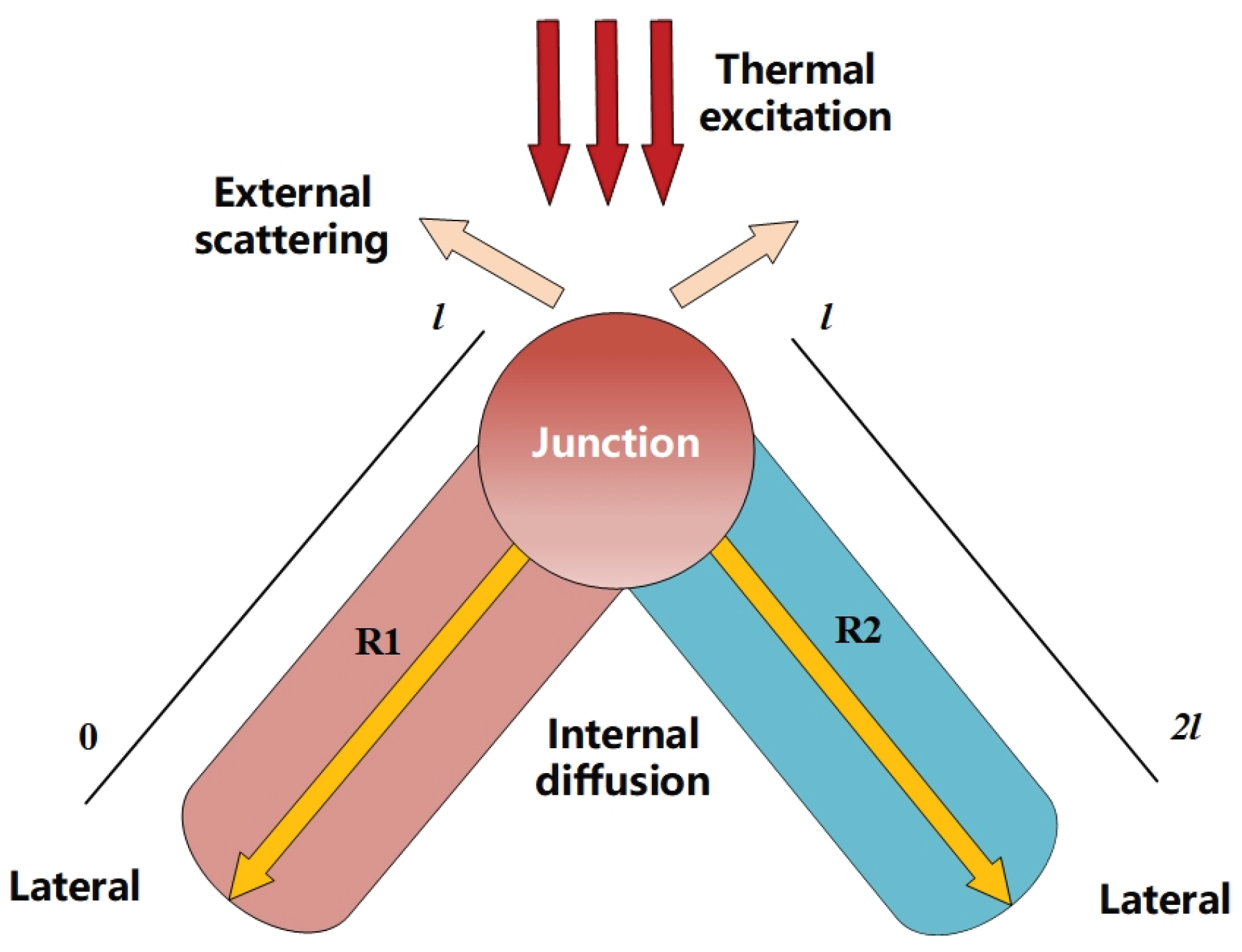
Figure 3.
CRBM-DBN-PINN framework.
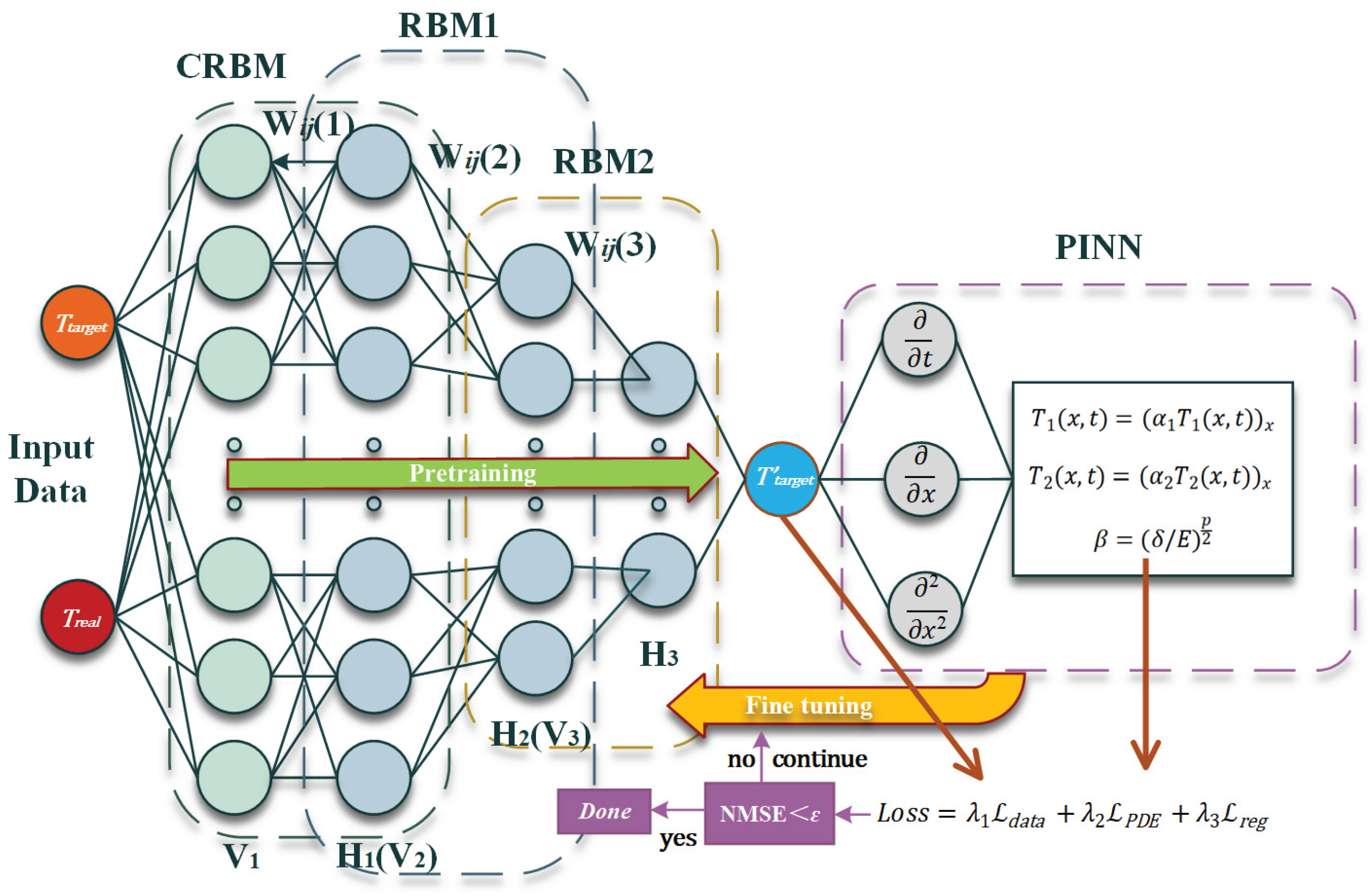
Figure 4.
Block diagram of the thermocouple dynamic calibration platform based on laser.
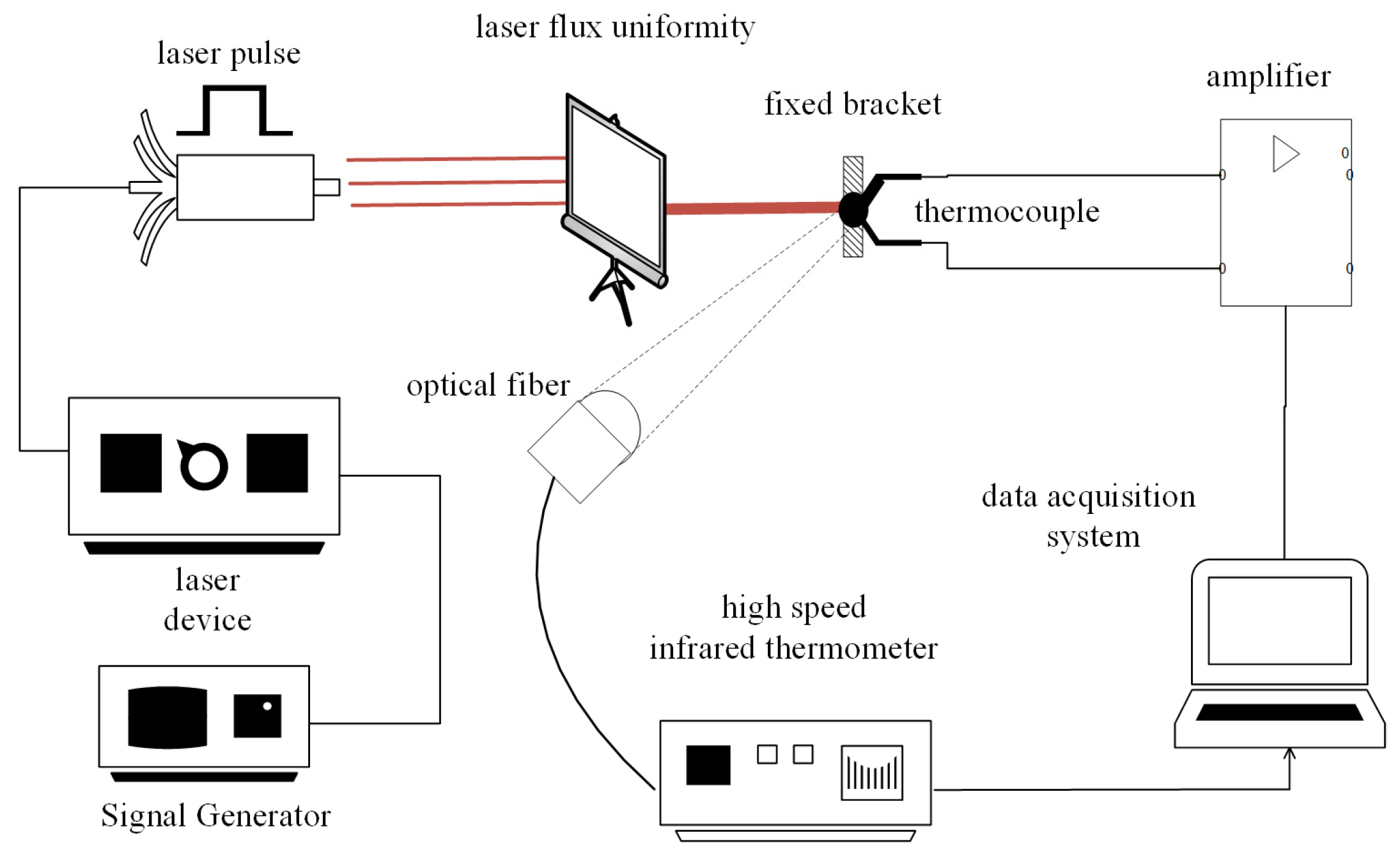
Figure 5.
Physical diagram of platform.
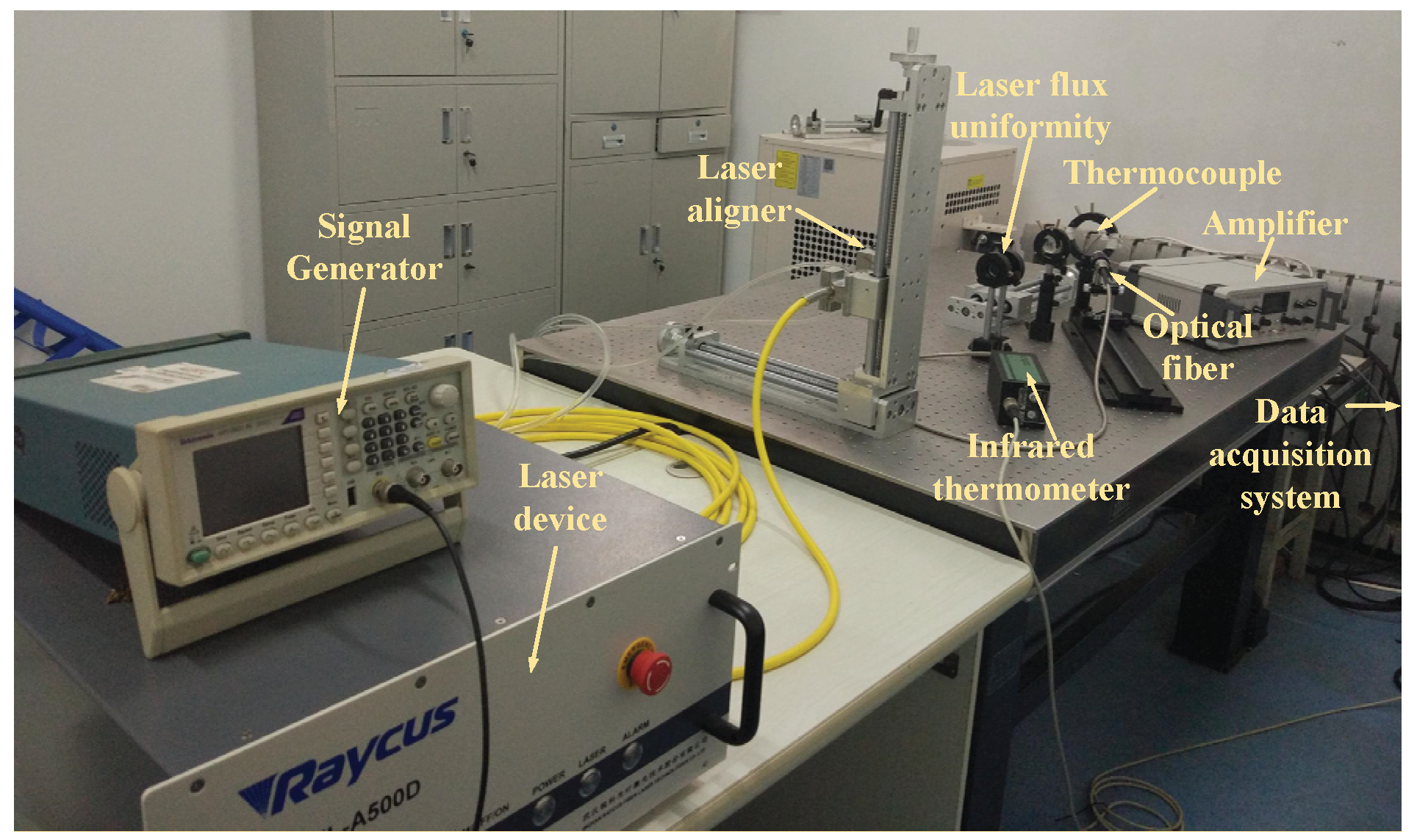
Figure 6.
The structural types of thermocouple junctions: (a) butt-welded structure; (b) ball-welded structure.
Figure 6.
The structural types of thermocouple junctions: (a) butt-welded structure; (b) ball-welded structure.
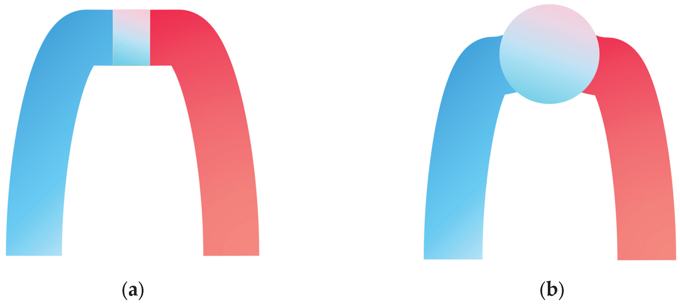
Figure 7.
Thermocouple excitation and response signals at different laser power.
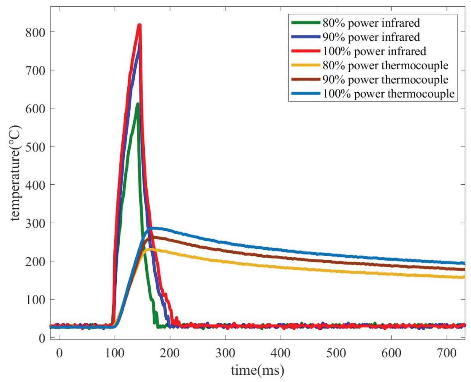
Figure 8.
Comparison of measured temperatures at fine-wire diameters of 0.25mm and 0.38mm.
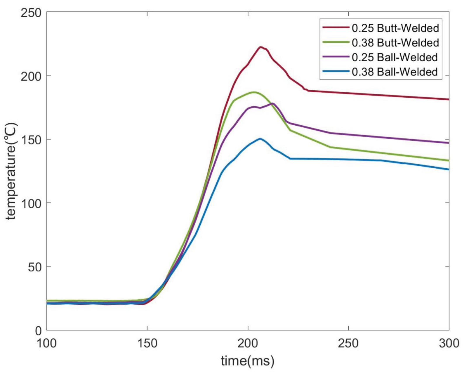
Figure 8.
The variations in network weights and hidden eigenvalues: (a) Removal of PINN; (b) Complete network.
Figure 8.
The variations in network weights and hidden eigenvalues: (a) Removal of PINN; (b) Complete network.
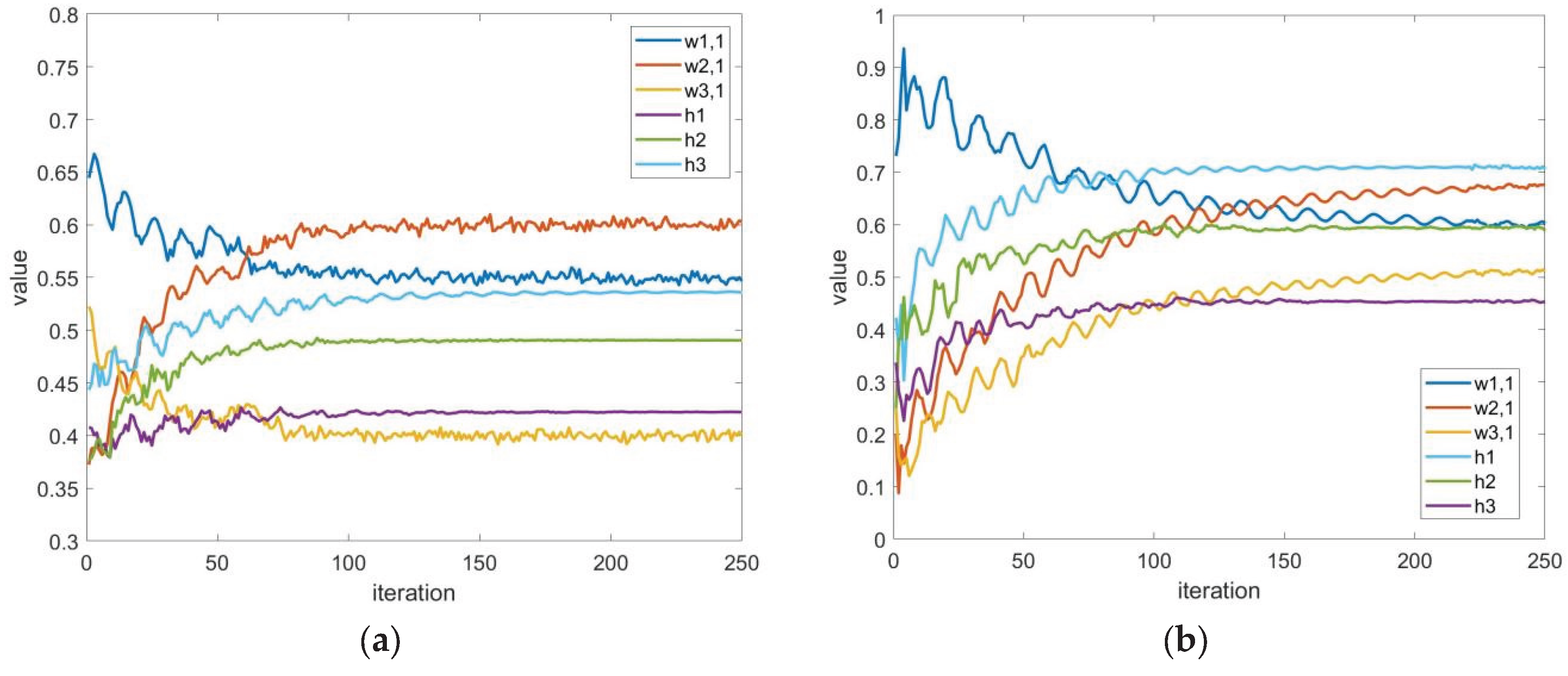
Figure 9.
Comparison of convergence results before and after ablation of PINN under Adam optimization.
Figure 9.
Comparison of convergence results before and after ablation of PINN under Adam optimization.
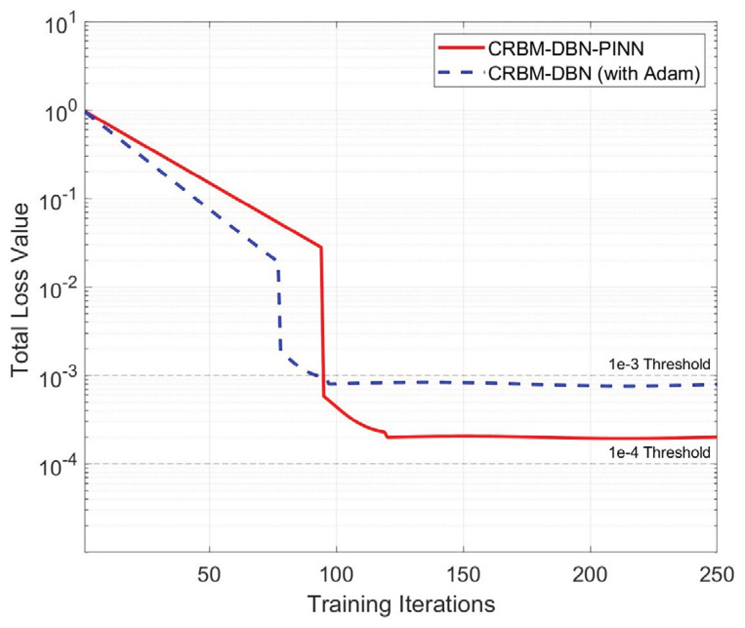
Figure 10.
The results of error correction for thermocouples at p=1, 3, and 7: (a) 0.25mm ball-welded thermocouple; (b) 0.25mm butt-welded one.
Figure 10.
The results of error correction for thermocouples at p=1, 3, and 7: (a) 0.25mm ball-welded thermocouple; (b) 0.25mm butt-welded one.
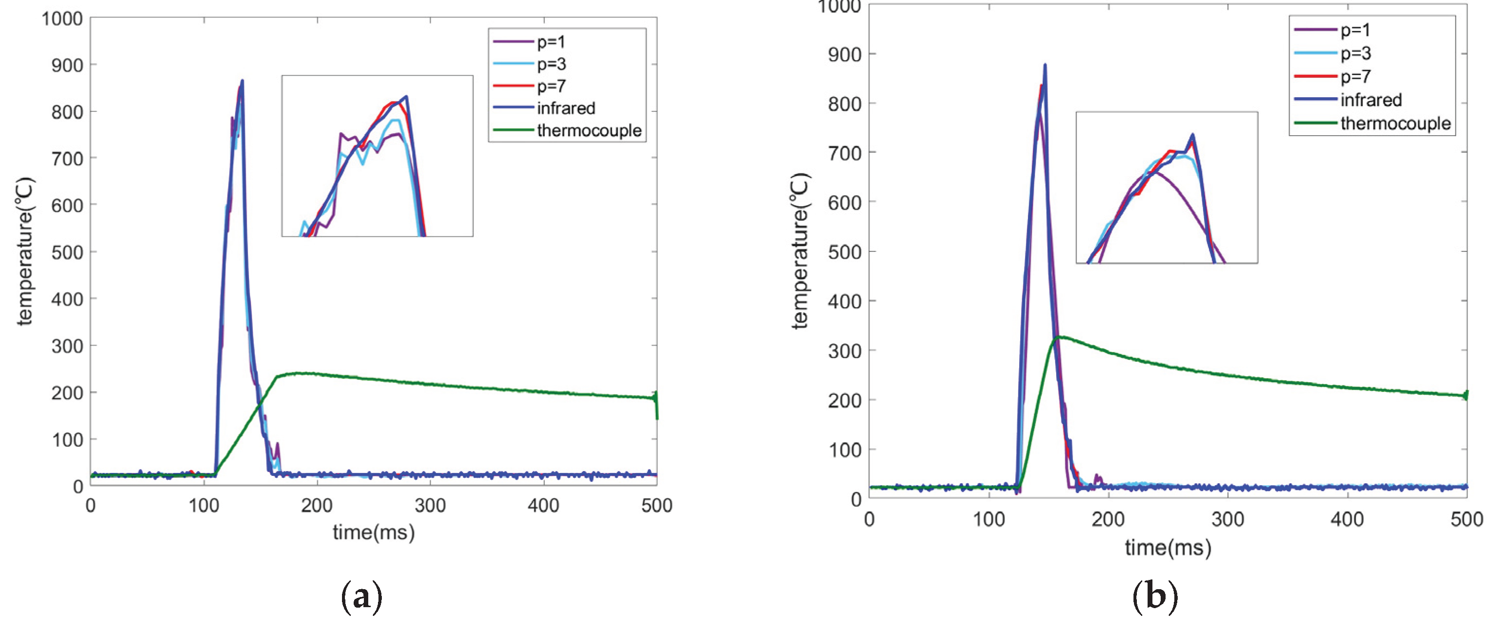
Figure 11.
The outcomes of test samples pre- and post-adjustment: (a) a comparison of ball-welded thermocouples between 0.25mm and 0.38mm; (b) a comparison of butt-welded thermocouples between 0.25mm and 0.38mm.
Figure 11.
The outcomes of test samples pre- and post-adjustment: (a) a comparison of ball-welded thermocouples between 0.25mm and 0.38mm; (b) a comparison of butt-welded thermocouples between 0.25mm and 0.38mm.
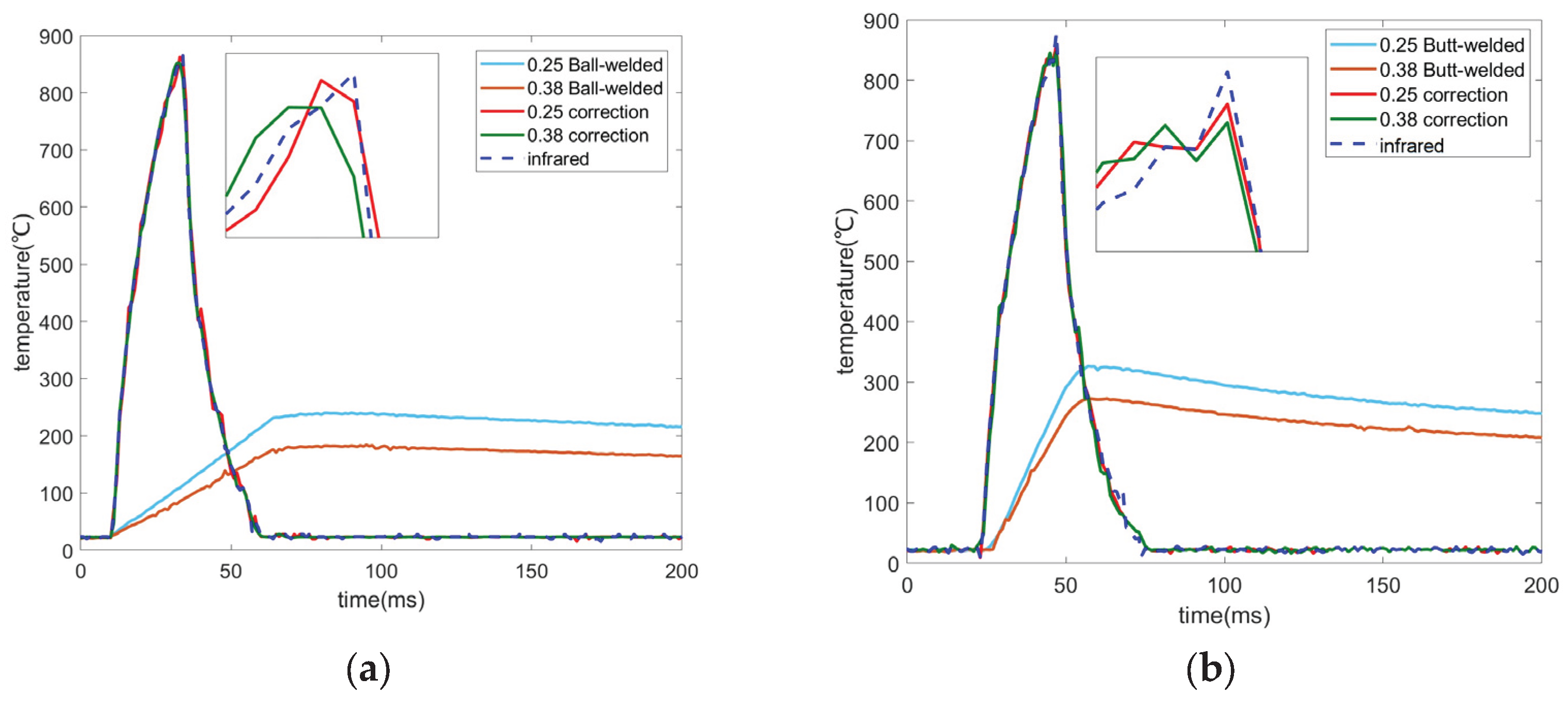
Figure 12.
Comparison of error correction results of different algorithms.
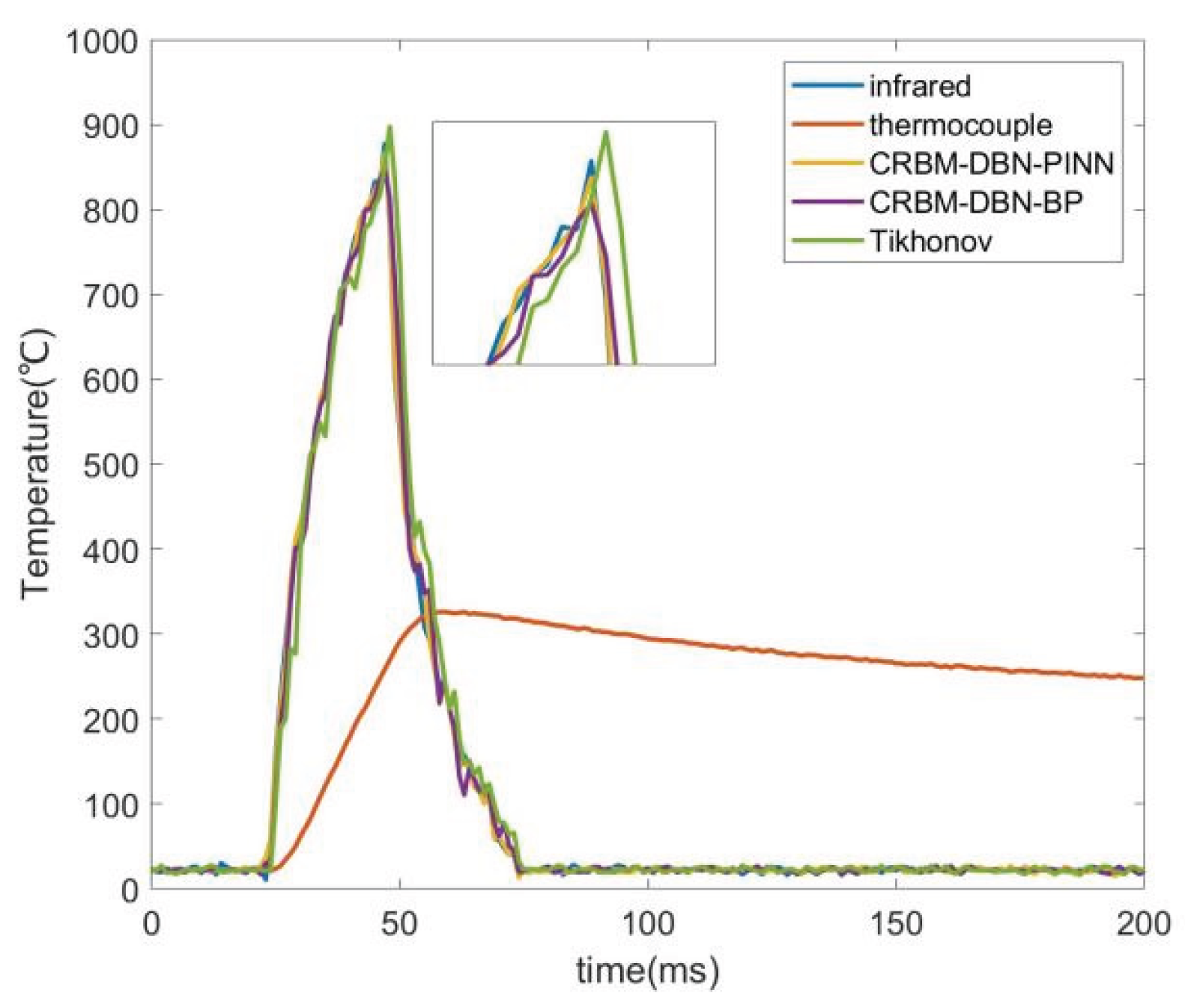
Figure 13.
Blast verification method: (a) Layout of measurement points; (b) Two kinds of thermocouple fixing methods.
Figure 13.
Blast verification method: (a) Layout of measurement points; (b) Two kinds of thermocouple fixing methods.
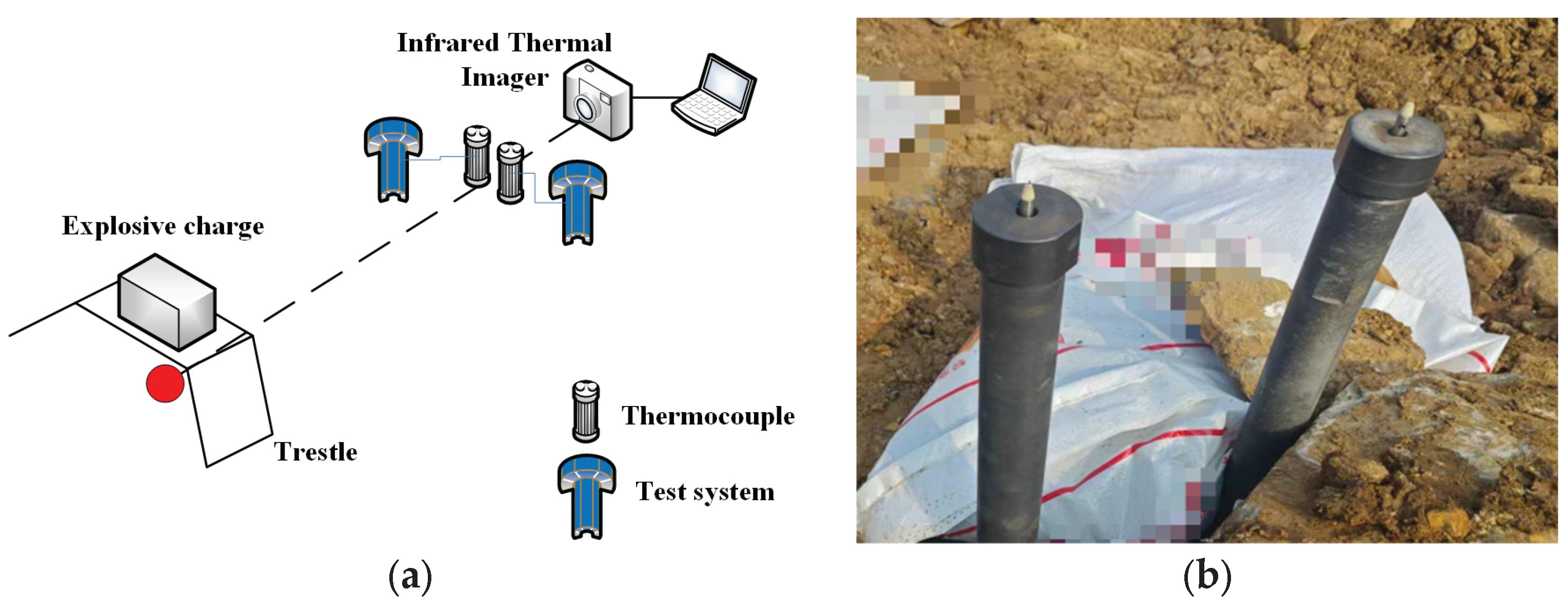
Figure 14.
Comparison of measured dynamic error correction results of two kinds of thermocouples.
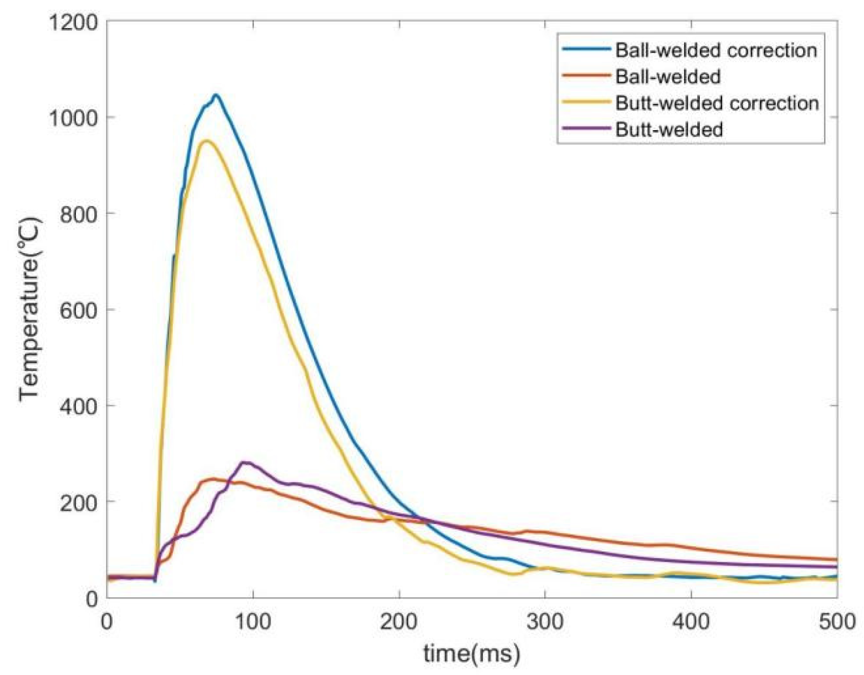

Table 1.
Temperature peak information for different thermocouple structures.
| p value | 0.25mmbutt-welded | 0.25mmball-welded | ||||
| Peak value (°C) | Infrared value (°C) | RE% | Peak value(°C) | Infrared value(°C) | RE% | |
| 1 | 790.0 | 878.6 | 10.1 | 783.8 | 865.2 | 9.4 |
| 3 | 831.3 | 5.4 | 814.0 | 5.9 | ||
| 7 | 858.1 | 2.3 | 852.3 | 1.5 | ||
Table 2.
Performance of CRBM-DBN-PINN model on different thermocouples with different structures.
| Junction | Average peak temperature (°C) | Average Infrared temperature (°C) | Peak relative error (%) | Risetime improved(ms) | R2 |
| 0.25mm butt-welded | 858.4 | 864.9 | 0.75 | 11 | 0.947 |
| 0.25mm ball-welded | 857.1 | 869.4 | 1.41 | 31 | 0.924 |
| 0.38mm butt-welded | 847.1 | 859.8 | 2.06 | 11 | 0.925 |
| 0.38mm ball-welded | 850.9 | 868.9 | 2.07 | 31 | 0.916 |
Table 3.
Comparison of performance of different algorithms on 0.25mm welded thermocouples.
| Correction algorithm | Average peak temperature (°C) | Averageinfrared temperature (°C) | Peak relative error (%) | Risetime improved(ms) | R2 |
| Tikhonov | 897.4 | 877.5 | -2.2 | 10 | 0.833 |
| CRBM-DBN-BP | 859.5 | 2.05 | 12 | 0.902 | |
| CRBM-DBN-PINN | 870.2 | 0.83 | 12 | 0.948 |
Table 4.
Characteristic Statistics of Detonation Test Results.
| Junction | Original peak (°C) | Corrected peak (°C) | Theoretical peak (°C) | RE% (original and theoretical) | RE% (revised and theoretical) | Risetime improved(ms) |
| Ball-welded | 273.4 | 949.9 | 1103.1 | 75.2% | 13.7% | 26 |
| Butt-welded | 246.5 | 1045.7 | 77.7% | 5.1% | 6 |
Disclaimer/Publisher’s Note: The statements, opinions and data contained in all publications are solely those of the individual author(s) and contributor(s) and not of MDPI and/or the editor(s). MDPI and/or the editor(s) disclaim responsibility for any injury to people or property resulting from any ideas, methods, instructions or products referred to in the content. |
© 2025 by the authors. Licensee MDPI, Basel, Switzerland. This article is an open access article distributed under the terms and conditions of the Creative Commons Attribution (CC BY) license (http://creativecommons.org/licenses/by/4.0/).
Copyright: This open access article is published under a Creative Commons CC BY 4.0 license, which permit the free download, distribution, and reuse, provided that the author and preprint are cited in any reuse.


