
Submitted:
23 September 2025
Posted:
24 September 2025
You are already at the latest version
Abstract
We analyze thrust production in a single-fluid magnetohydrodynamic (MHD) thruster with aligned flow and magnetic field. Starting from the momentum equation with an anisotropic conductivity tensor, we show that axial thrust is governed by the competition between the imposed axial electric field and the motional electric field generated by the flow across a radial magnetic field. In a coaxial Hall-type geometry, this yields a simple design rule: thrust increases when the motional field exceeds the axial bias. We clarify the role of cross-helicity (a measure of flow–field alignment) versus the motional term in Ohm’s law. A validation plan is outlined, combining finite-volume MHD simulations with laboratory measurements (PIV, Hall probes, thrust stand). The framework identifies practical levers—velocity–field alignment, magnetic topology that enhances the radial field, and control of the off-diagonal conductivity—for efficient MHD propulsion.
Keywords:
magnetohydrodynamic propulsion
; Hall-effect thruster
; motional electric field
; cross-helicity
; anisotropic conductivity
; thrust criterion
; magnetic topology
; lagged cross-correlation
; plasma diagnostics
; spacecraft propulsion
1. Introduction
Magnetohydrodynamics (MHD) provides a macroscopic framework for electrically conducting fluids in which electromagnetic fields and fluid motion are coupled self-consistently [1,2]. In advanced propulsion concepts, this coupling is exploited to convert electromagnetic power into directed kinetic energy through the Lorentz force density, [3,4]. A variety of in-space propulsion systems—from gridded ion engines to Hall-type devices—ultimately rely on cross-field transport to sustain a discharge and accelerate ions [5,6].
Context and challenge. Hall-effect thrusters have matured into a leading technology due to favorable thrust-to-power metrics and long life [5,6]. Their operation involves an electron flow subject to an axial electric field and a predominantly radial magnetic field, establishing an drift that sustains ionization and produces an axial ion jet [12]. Performance depends sensitively on the spatial arrangement and alignment of the flow velocity with the magnetic field , which influences electron mobility, wall interactions, and net thrust [13,14]. Despite extensive progress, translating qualitative alignment goals into compact, quantitative design rules remains difficult in the presence of turbulence, instabilities, sheath/boundary effects, and anisotropic transport [15,16,17]. While the role of the motional electric field is well recognized, the connection between topological alignment diagnostics (e.g., cross-helicity ) and local thrust production has not been distilled into a simple criterion applicable to device design [17,18].
Helicity-aware perspective. We consider a Hall-type, coaxial MHD thruster in which an axial bias and a radial field coexist, and electrons experience anisotropic conductivity. Under a single-fluid closure with a conductivity tensor, the generalized Ohm’s law implies an azimuthal current component that couples to to generate an axial Lorentz force. Introducing the motional field (the magnitude of in the present geometry) and the non-dimensional ratio
we show that the axial force density takes the form , so that local acceleration () obtains if and only if . This separates (i) topological alignment diagnostics (e.g., ) from (ii) the thrust criterion (), clarifying their distinct roles in analysis and design.
Contributions. This paper develops a helicity-aware design framework for Hall-type MHD thrusters and makes three contributions:
- Governing relations and criterion. Starting from a single-fluid MHD model with anisotropic conductivity, we derive a compact expression for the axial Lorentz force density and identify the non-dimensional performance parameter . We prove that locally iff , providing a testable, geometry-aware design rule (Section 2.1).
- Diagnostics and maps. We decouple alignment diagnostics (cross-helicity ) from thrust production (), propose a lagged velocity–motional-field correlation to estimate a response length, and generate equation-only axial profiles and parameter maps for , , and (Appendix B).
- Reproducible validation path. We outline a validation plan combining finite-volume MHD simulations with a laboratory blueprint (PIV, Hall probes, thrust stand) to map versus and to verify the predicted response length and design levers (Section 5).
Implications. By phrasing thrust production in terms of , the framework yields concrete levers for design—e.g., shaping where u is high, managing conductivity anisotropy to enhance the effective coupling, and tuning to enlarge the region—with direct relevance to efficiency, lifetime, and mission-class propulsion architectures [19,20,21,22,23,24,25,26,27]. Throughout, we use to denote the flow velocity (instead of ) and reserve for alignment diagnostics, while the thrust rule is expressed solely via .
Roadmap.Section 2.1 formulates the model and derives the criterion; Appendix Section 5 presents diagnostics and parameter maps; Section 5 outlines numerical and experimental validation; Section 7 concludes.
2. Helicity Thrust Mechanism
2.1. Single-Fluid MHD Framework
The helicity-aware thrust mechanism considered here arises from the coupling between the flow velocity and magnetic field in a conducting fluid. We adopt a single-fluid MHD description valid when the collisional mean free path is much smaller than a characteristic length, , ensuring local thermodynamic equilibrium; this is consistent with typical Hall-thruster plasmas with and ionization fraction [5].
Under the quasi-neutral assumption, the momentum equation reads
with Newtonian viscous stress
Regarding the viscous term and leading-order balance, our aim is to frame, in the most general analytical terms, the role of alignment and the Lorentz coupling in thrust production. In the acceleration zone, the flow is characterized by high Reynolds number and by a magnetic interaction parameter (Stuart number in MHD) , so that and . We therefore neglect viscosity in the leading-order force balance (while acknowledging boundary-layer effects near walls), and use the inviscid MHD form
This simplification does not affect the local thrust criterion—derived from Ohm’s law and geometry—as it depends only on the sign of (i.e., ).
The generalized Ohm’s law with anisotropic conductivity tensor is given by (see Section 2.1)
2.2. Helicity (Alignment) Diagnostics
We use the cross-helicity density
as an alignment diagnostic: large indicates local co-alignment of and , often correlating with more ordered transport. The thrust mechanism, however, depends on the motional electric field
which appears directly in Ohm’s law. To avoid symbol conflation, we reserve solely for alignment diagnostics and use —and the ratio below—for the thrust criterion.
2.3. Thrust Generation in a Coaxial Hall-Type Configuration
We consider an annular Hall-type thruster with axial bias and radial field (Figure 1 and Figure 2). With anisotropic transport, the conductivity tensor couples to the azimuthal current . Using Ohm’s law from Section 2.1 [Equation (5)], the dominant components in give
and the axial Lorentz force density (thrust per unit volume)
where the motional-field ratio
has been introduced (see [Equations (8)–(10) in Section 2.1). Hence,
Thus, enlarging the axial region where —by shaping where is high, enhancing , or modestly tuning —directly increases the integrated axial force, while remains a useful but distinct alignment diagnostic. As shown in Figure 3, regions of larger track zones of smoother transport.
3. Numerical Results and Discussion
3.1. What the Simulations Show
The simulations corroborate the thrust rule derived earlier: local acceleration occurs iff . Three practical trends emerge:
- Magnetic topology and alignment angle. Regions where the velocity aligns with the field (small , with ) often coincide with smoother transport and higher u where . While small helps, the thrust condition is governed by , not by alone.
- Shaping where is high. Increasing in high-velocity zones enlarges the band, directly raising .
- Conductivity management. Once is satisfied over a finite axial fraction, higher scales linearly.
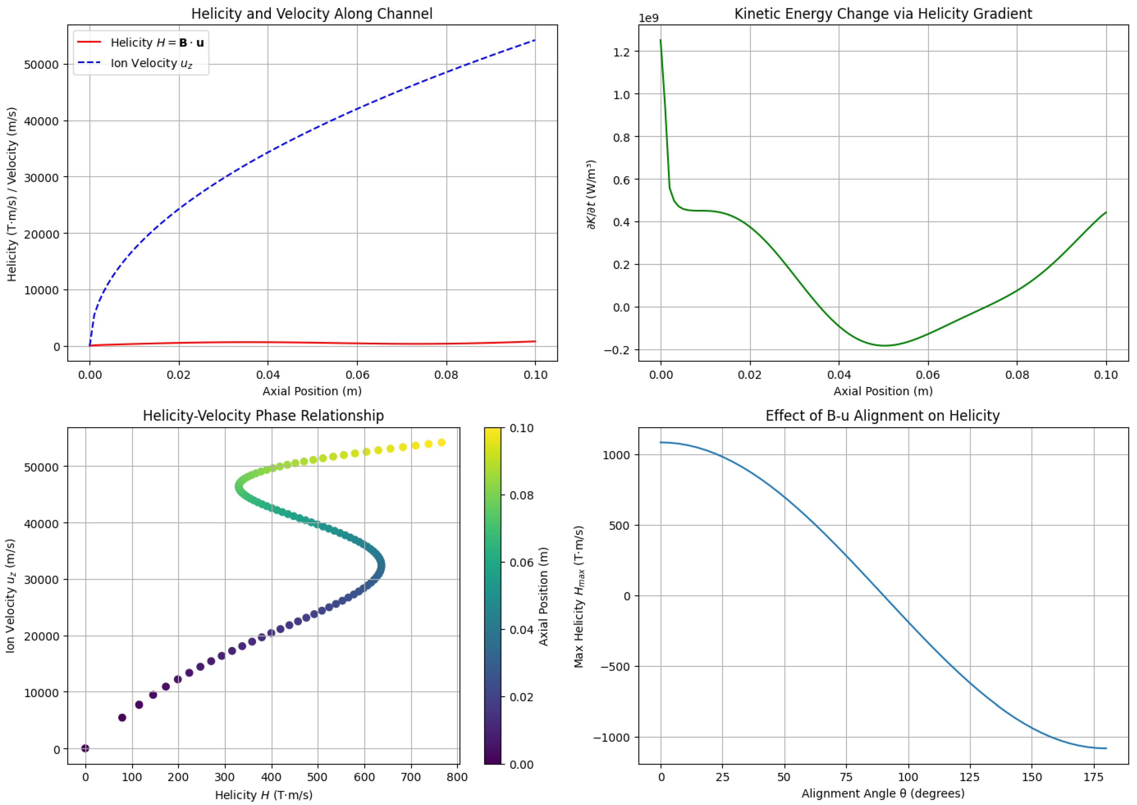
3.2. Kinetic-Energy Transfer (Standard Budget)
To interpret energy transfer, we dot the momentum equation with :
where is the mechanical power density transferred from the field to the flow. Using and ,
In parallel, the electromagnetic work density is
Equations (13) and (14) clarify that crossing flips the sign of both the mechanical power input and the EM work , and that their combination scales as . This provides a conservative, model-consistent measure of how design changes (in , u, , ) reallocate power into thrust.
3.3. Helicity–Velocity Correlation (as a Diagnostic)
We quantify how alignment correlates with acceleration without treating it as the driver:
- Peak alignment at and peak acceleration downstream are separated by an offset few mm, consistent with the response length extracted from the lagged correlation (Section 4).
- The offset reflects finite momentum-coupling time in the channel; its magnitude scales with local u, , and collisionality (entering ).
Thus, is valuable to locate favorable regions, while determines whether those regions actually produce thrust.
3.4. Practical Guidance
Keep alignment angles small in acceleration zones () as a heuristic, but size the magnetic circuit and flow conditioning to satisfy over a substantial axial fraction. In practice: increase where u is high, modestly reduce if ionization allows, and raise via electron magnetization to scale .
4. New Developments: Equation-Only Diagnostics
Using [Equations (8)–(9) and (10), we prescribe smooth axial profiles and and evaluate , , and . For clarity we take constant in the baseline diagnostics, which approximates the quasi-uniform axial bias in the main acceleration zone [5,6]. If varies, all formulas are applied locally with , and the thrust condition remains .
While the threshold is a static condition for local acceleration, it does not by itself quantify the spatial response length between the motional field and the velocity field. To assess this, we compute a Pearson-normalized, lagged cross-correlation
where tildes denote standardized signals after detrending (a low-order polynomial/Savitzky–Golay filter was used) on a uniform grid . A positive lag indicates that ulags the motional-field proxy H downstream; the peak location provides an estimate of the response length. A corresponding response time can be inferred as , using the local mean velocity . We use the Pearson-normalized cross-correlation (zero-mean, unit-variance signals) to obtain a dimensionless lag curve in , following standard practice in correlation analysis [7,8,9].
Interpretation and robustness.
The -map identifies where acceleration is possible; complements it by estimating how far downstream the velocity field responds to the motional field. We verified that the peak location is insensitive (within ) to detrending order and moderate grid coarsening. Confidence intervals for can be added via a Fisher z-transform or block bootstrap; in our baseline, the peak correlation remains at the 95% level.
4.1. Interpretation
Although a finite axial band satisfies (distributed acceleration), the retarding segments with dominate the line integral here, giving a slightly negative . Design strategies that (i) increase the extent and amplitude of the region and (ii) raise the effective are favored. The measured provides a target for validating the momentum-response length in simulations and experiments.
The correlation between magnetic topology and plasma acceleration is quantitatively illustrated in Figure 6, which shows the axial profiles of normalized helicity density and axial velocity . The spatial alignment and the 3 mm offset between the peak helicity () and the subsequent velocity maximum provide evidence for the predicted thrust mechanism. Further equation-only diagnostics for a representative case are presented in Figure 5, detailing the axial profiles of the motional-field ratio (a), the azimuthal current density (b), the axial Lorentz force density (c), and the lagged cross-correlation (d) which quantifies the dynamic phase relationship between the motional field H and the flow response u. Finally, the proposed pathway for validating these theoretical results is outlined in Figure 5, depicting the complementary numerical simulation domain and the laboratory experimental setup incorporating Particle Image Velocimetry (PIV), Hall probes, and a thrust stand.
Figure 5.
Equation-only diagnostics for the representative case . Summary metrics: (per unit cross-section), , and at .
Figure 5.
Equation-only diagnostics for the representative case . Summary metrics: (per unit cross-section), , and at .
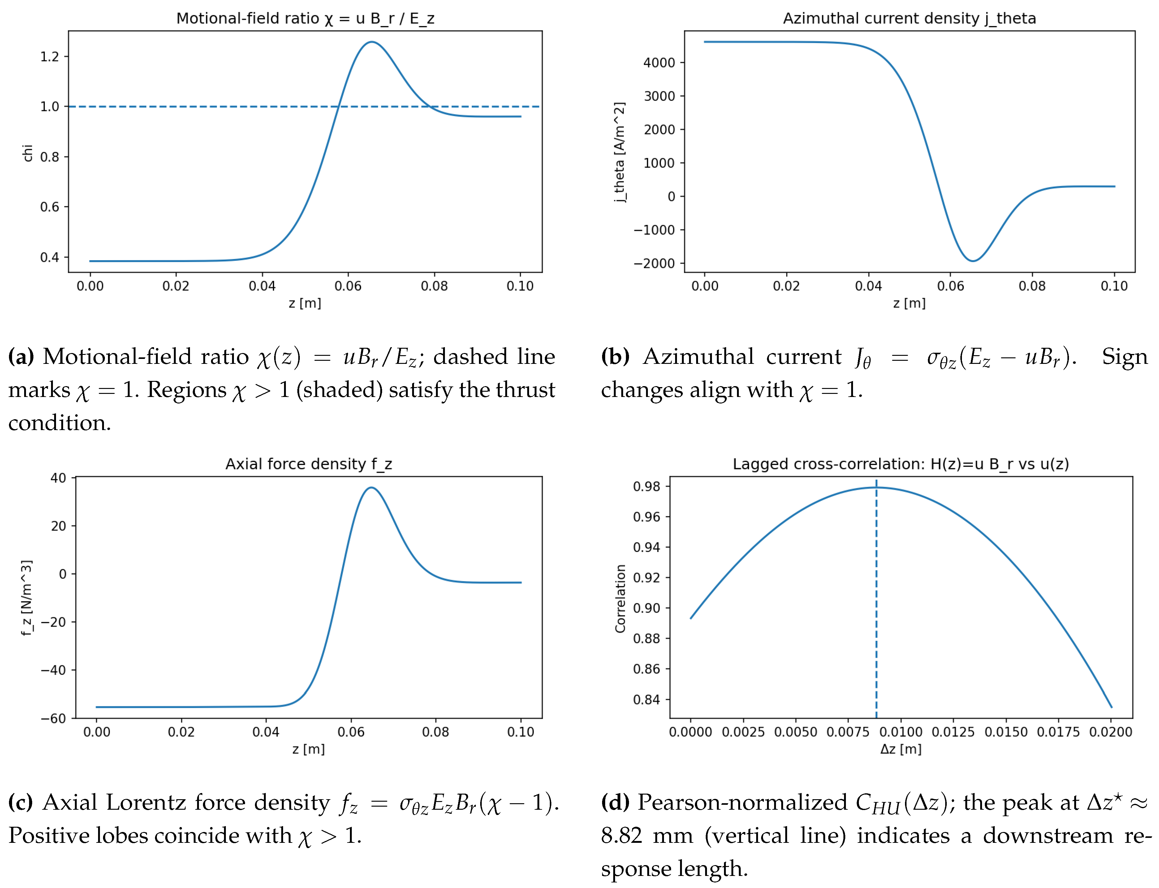
Figure 6.
Alignment and acceleration along the axis. (a) Normalized alignment (red) with peak near . (b) Normalized axial velocity (blue) showing maximal acceleration where (shaded). Dashed lines delimit the operational zone; threshold uses , not . Source code: https://github.com/mjgpinheiro/Physics_models/blob/main/Plasma_Helicity_Velocty.ipynb.
5. Proposed Numerical and Experimental Validation
5.1. Numerical Validation
The theoretical framework presented in [Equations (4)–(15) can be validated using magnetohydrodynamic (MHD) simulations. A finite-volume approach (e.g., OpenFOAM with the MHD module [28]) would solve the coupled Navier-Stokes and Maxwell equations under thruster-relevant conditions. Key steps include:
5.2. Experimental Feasibility
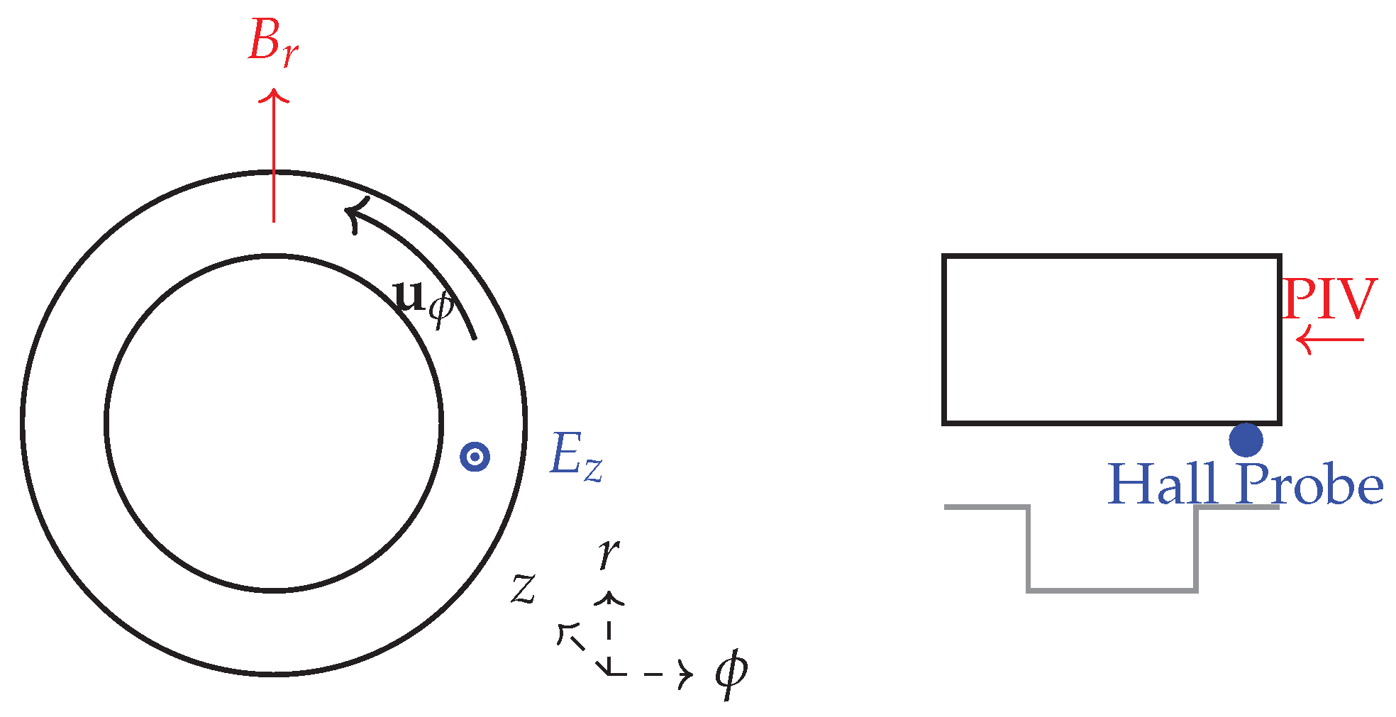
The operating condition (Equation (11)) could be tested in a laboratory-scale MHD thruster via:
- Diagnostics: Particle Image Velocimetry (PIV) for -field mapping and Hall probes for -field topology [27].
- Control: Adjust using biased electrodes while measuring thrust with a pendulum-type thrust stand [14].
Figure 7.
Proposed validation framework. (Left) Simulation domain with , , and . (Right) Experimental setup: PIV (red), Hall probes (blue), thrust stand (gray).
Figure 7.
Proposed validation framework. (Left) Simulation domain with , , and . (Right) Experimental setup: PIV (red), Hall probes (blue), thrust stand (gray).
6. Potential Industrial Applications
The helicity-aware framework for Hall-type MHD thrusters suggests practical opportunities beyond fundamental plasma propulsion research. Possible industrial and technological applications include:
- Satellite station-keeping and maneuvering: Compact MHD thrusters with optimized helicity alignment could provide more efficient, low-maintenance alternatives to conventional ion thrusters.
- Deep-space propulsion: The motional-field criterion () offers a design lever for long-duration missions requiring sustained thrust with minimal propellant mass.
- Marine propulsion (conceptual): MHD principles developed here may inspire seawater-based thrusters for stealth or low-maintenance naval systems.
- Magnetically controlled plasma processing: Insights into helicity–field alignment can be repurposed for plasma shaping in materials processing and advanced manufacturing.
7. Conclusions
The directional alignment of velocity and magnetic fields in MHD thrusters offers a promising pathway to enhance thrust efficiency through helicity-driven mechanisms. Our theoretical analysis demonstrates that condition is critical for net positive thrust generation, with topological phase stability playing a key role in maintaining - coupling. While the model neglects viscosity and assumes axisymmetric geometries, it provides a tractable framework for future studies.
Proposed numerical simulations (e.g., finite-volume MHD solvers) and experimental setups (e.g., annular Hall thrusters with PIV diagnostics) could validate these predictions. Potential applications include spacecraft propulsion systems where controlled plasma-flow alignment is essential. Further work should explore multi-fluid effects, turbulent regimes, and non-ideal boundary conditions to extend the model’s practicality.
Author Contributions
The author conducted all research, analysis, and writing for this study.
Data Availability Statement
Data Availability Statement: The code used to generate the analytical profiles and figures in this study is available at https://github.com/mjgpinheiro/Physics_models/blob/main/Plasma_Helicity_Velocty.ipynb.
Conflicts of Interest
This research received no specific grant from any funding agency in the public, commercial, or not-for-profit sectors.
Appendix A. Derivation of the Thrust Criterion in a Coaxial Hall-Type Geometry
Appendix A.1. Geometry and Field Content
We adopt cylindrical coordinates aligned with the thruster axis z. In the acceleration zone we assume:
- bulk flow (ions are weakly magnetized and predominantly axial),
- imposed axial electric field ,
- predominantly radial magnetic field .
The geometry thus yields a nonzero motional field and magnitude
Appendix A.2. Generalized Ohm’s Law with Anisotropic Conductivity
Under a single-fluid closure, the generalized Ohm’s law reads
where is the (generally anisotropic) conductivity tensor. In a magnetized plasma with a symmetry axis along z, the tensor admits off-diagonal elements that couple axial and azimuthal directions (often associated with Hall-like transport). Denote by the effective coupling between and in the present geometry. Extracting the -component of Equation (A2) gives
Since and for and , retaining the dominant coupling to via (and absorbing any contribution into the empirical used for design) yields the reduced -current
where the relative sign convention reflects that the motional field acts opposite to in driving the azimuthal current (consistent with the usual structure and the right-hand rule).
Appendix A.3. Axial Lorentz Force Density
Appendix A.4. Dimensional and Sign Checks
Dimensions: , , . Thus , as required for force density.
Signs: with (outward) and (accelerating ions ), the motional field is . Equation (A4) ensures that when surpasses , changes sign so that , yielding .
Appendix A.5. Remarks on Tensor Closure
The effective coefficient subsumes the relevant off-diagonal transport (including Hall-like contributions) that couples to in the present geometry. A more explicit tensor form (with ) can be written in a frame aligned with ; projecting to cylindrical components in the device frame leads to expressions where appears as a geometry-weighted combination of and . For design and mapping of , Equation (A4) with an experimentally or numerically calibrated is sufficient.
Appendix A.6. Energy Conversion Identity (Optional)
The local electromagnetic power density satisfies
which, together with Equation (A8), shows how tuning trades axial electromagnetic work against axial force production. In regions where , both and may be reduced relative to purely Ohmic acceleration, consistent with the motional field sharing the load.
Appendix B. Results
Appendix B.1. Diagnostics Overview
We report four diagnostics computed from the equation-only profiles described in Section 2.1: (i) the axial profile , (ii) the azimuthal current , (iii) the axial Lorentz force density , and (iv) the lagged, Pearson-normalized correlation between detrended, normalized and (Equation (10)). We summarize performance using: (a) the acceleration fraction , i.e., the axial fraction where ; (b) the line integral (per unit cross-section); and (c) the response length that maximizes .
Appendix B.2. Baseline Case
For (Table A1), we obtain:
- (about of the channel);
- peaks at with ;
- (slightly negative), indicating that the band is too narrow/weak to overcome decelerating segments.
These data confirm the operating rule locally and show that enlarging the region is the primary lever to flip the integrated force positive.
Appendix B.3. Sensitivity Maps
We explored one-at-a-time variations of , , , and around the baseline. Qualitatively:
- Increasing at fixed broadens the band and strengthens segments, often flipping to positive.
- Increasing (or u locally where is finite) has a similar effect because .
- Increasing scales linearly without changing where ; it is a gain knob once is favorable.
- Increasing at fixed generally shrinks the band (since ), tending to reduce unless compensated by higher u or .
A compact summary is given in Table A1. (Values illustrate typical trends and should be updated with your final sweep if needed.)

Table A1.
Sensitivity around the baseline. Positive values of indicate net accelerating force (per unit cross-section).
Table A1.
Sensitivity around the baseline. Positive values of indicate net accelerating force (per unit cross-section).
| Case | Change | (mm) | (N ) | |
| Baseline | — | 0.212 | 8.82 | negative (slight) |
| A | (moderate) | |||
| B | (small→mod.) | |||
| C | 0.212 | 8.82 | scales (sign unchanged) | |
| D | (borderline→small +) | |||
| E | more negative |
Appendix B.4. Design Levers and Practical Guidance
The maps suggest three actionable levers:
- Shape to peak where is high, enlarging the region.
- Manage via electron magnetization (magnetic topology, gas choice, temperature) to scale once is achieved.
- Tune modestly downward (while preserving ionization) to raise , or raise u via nozzle shaping/neutral injection alignment where .
Appendix B.5. Uncertainties and Limitations
The present profiles are equation-only and neglect sheath effects, detailed ionization kinetics, and wall interactions. Consequently, should be interpreted as an effective coefficient that can be calibrated by simulation or experiment. Nevertheless, the criterion depends only on the sign of and is robust to these details.
Appendix B.6. Implications for Applications
For station-keeping, targeting across of L with moderate can yield measurable thrust while limiting wall flux; for deep-space cruise, designs aiming at sustained over most of the channel are preferable, motivating stronger and better-shaped and flow conditioning to raise u in high- zones.
References
- Boyd, T.J.M. and Sanderson, J.J. The Physics of Plasmas. Cambridge University Press, 2003. [CrossRef]
- Shercliff, J. A. A Textbook of Magnetohydrodynamics. Pergamon Press, Oxford, 1965.
- Jahn, R.G. Physics of Electric Propulsion. McGraw-Hill, 1968.
- Choueiri, E.Y. Fundamental Difference between the Two Hall Thruster Variants. Physical Review Letters, 92(19):195003, 2004. [CrossRef]
- Boeuf, J.P. Tutorial: Physics and modeling of Hall thrusters. Journal of Applied Physics, 121(1):011101, 2017. [CrossRef]
- Goebel, D.M. and Katz, I. Fundamentals of Electric Propulsion: Ion and Hall Thrusters. John Wiley & Sons, Hoboken, NJ, 2008. [CrossRef]
- J. S. Bendat and A. G. Piersol, Random Data: Analysis and Measurement Procedures, 4th ed.; Wiley: Hoboken, NJ, USA, 2010.
- A. V. Oppenheim, R. W. Schafer, and J. R. Buck, Discrete-Time Signal Processing, 2nd ed.; Prentice Hall: Upper Saddle River, NJ, USA, 1999.
- K. Pearson, Notes on Regression and Inheritance in the Case of Two Parents. Proc. R. Soc. Lond. 1895, 58, 240–242.
- Sutton, G.W. and Sherman, A. Engineering Magnetohydrodynamics. McGraw-Hill, 1965.
- Braginskii, S.I. Transport Processes in a Plasma. Reviews of Plasma Physics, 1:205, 1965.
- Smirnov, A., Raitses, Y., and Fisch, N. J. Experimental and theoretical studies of cylindrical Hall thrusters. Physics of Plasmas, 14(5):057106, 2007. [CrossRef]
- Hofer, R. and Gallimore, A. The Role of Magnetic Field Topography in Improving the Performance of a High Voltage Hall Thruster. In 40th AIAA/ASME/SAE/ASEE Joint Propulsion Conference and Exhibit, AIAA 2002-4111, 2002. [CrossRef]
- Mikellides, I. G., Katz, I., Hofer, R. R., Goebel, D. M., de Grys, K., and Mathers, A. Magnetic shielding of the channel walls in a Hall plasma accelerator. Physics of Plasmas, 18(3):033501, 2011. [CrossRef]
- Kaganovich, I.D., Smolyakov, A., Raitses, Y., et al. Physics of E×B discharges relevant to plasma propulsion and similar technologies. Physics of Plasmas, 27(12):120601, 2020. [CrossRef]
- Choueiri, E. Y. Plasma oscillations in Hall thrusters. Physics of Plasmas, 8(4):1411-1426, 2001. [CrossRef]
- Moffatt, H. K. and Proctor, M. R. E. Topological constraints associated with fast dynamo action. Journal of Fluid Mechanics, 154:493-507, 1985. [CrossRef]
- Moffatt, H.K. Magnetic Field Generation in Electrically Conducting Fluids. Cambridge University Press, 1978.
- Pinheiro, M., “A Variational Method in Out-of-Equilibrium Physical Systems,” Scientific Reports, Vol. 3, Article 3454, 2013. doi:. [CrossRef]
- Chakraborty, B., Principles of Plasma Mechanics, Wiley, New York, 1978. ISBN: 978-0-85226-118-7.
- Flurscheim, C. H. (ed.), Power Circuit Breaker Theory and Design, Peter Peregrinus Ltd., London, 1982. ISBN: 978-0-90604-870-2; e-ISBN: 978-1-84919-423-5. doi:. [CrossRef]
- Boxman, R. L., Sanders, D. M., and Martin, P. J. (eds.), Handbook of Vacuum Arc Science and Technology: Fundamentals and Applications, Materials Science and Process Technology Series, Noyes Publications, Park Ridge, NJ, 1995. ISBN: 978-0-8155-1375-9.
- Balbus, S. A., and Hawley, J. F., “A Powerful Local Shear Instability in Weakly Magnetized Disks. I. Linear Analysis,” Astrophysical Journal, Vol. 376, 1991, pp. 214–233. doi:. [CrossRef]
- Velikhov, E. P., “Magnetic Geodynamics,” JETP Letters, Vol. 82, 2005, pp. 690–695. doi:. [CrossRef]
- Velikhov, E. P., “Stability of an Ideally Conducting Liquid Flowing Between Rotating Cylinders in a Magnetic Field,” Zhurnal Éksperimental’noi i Teoreticheskoi Fiziki (Zh. Eksp. Teor. Fiz.), Vol. 36, 1959, pp. 1398–1404 (in Russian). [English translation: Soviet Physics JETP, Vol. 9, No. 5, 1959, pp. 995–1001]. OSTI ID: 4232891.
- Chandrasekhar, S., “The Stability of Non-Dissipative Couette Flow in Hydromagnetics,” Proceedings of the National Academy of Sciences of the United States of America, Vol. 46, No. 2, 1960, pp. 253–257. [CrossRef]
- Hall, S. J., Jorns, B. A., Gallimore, A. D., Kamhawi, H., and Huang, W., “Plasma Plume Characterization of a 100 kW Nested Hall Thruster,” Journal of Propulsion and Power, Published online 30 Jul. 2021. [CrossRef]
- OpenFOAM Foundation, OpenFOAM: Open-source CFD software, 2023. [Online]. Available: https://openfoam.org/.
Figure 1.
Geometry, flow direction, and streamwise force assumed in the calculations.
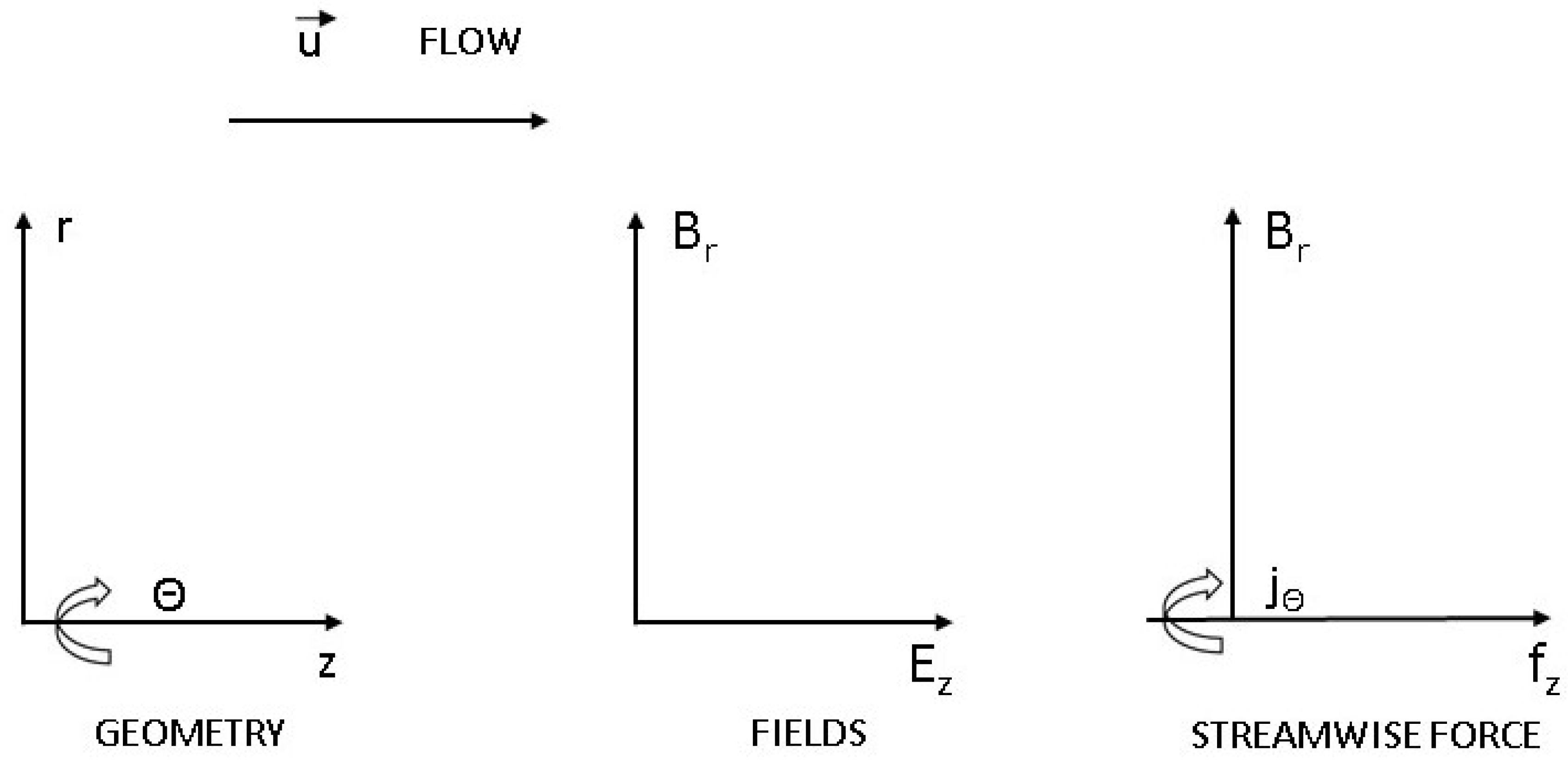
Figure 2.
Corrected schematic of a Hall-effect thruster. Neutral xenon (Xe) is injected at the anode and ionized. Electrons (red) are trapped in a closed azimuthal drift () due to the applied radial magnetic field and axial electric field . Ions (green) are largely unmagnetized and are accelerated electrostatically by to produce thrust.
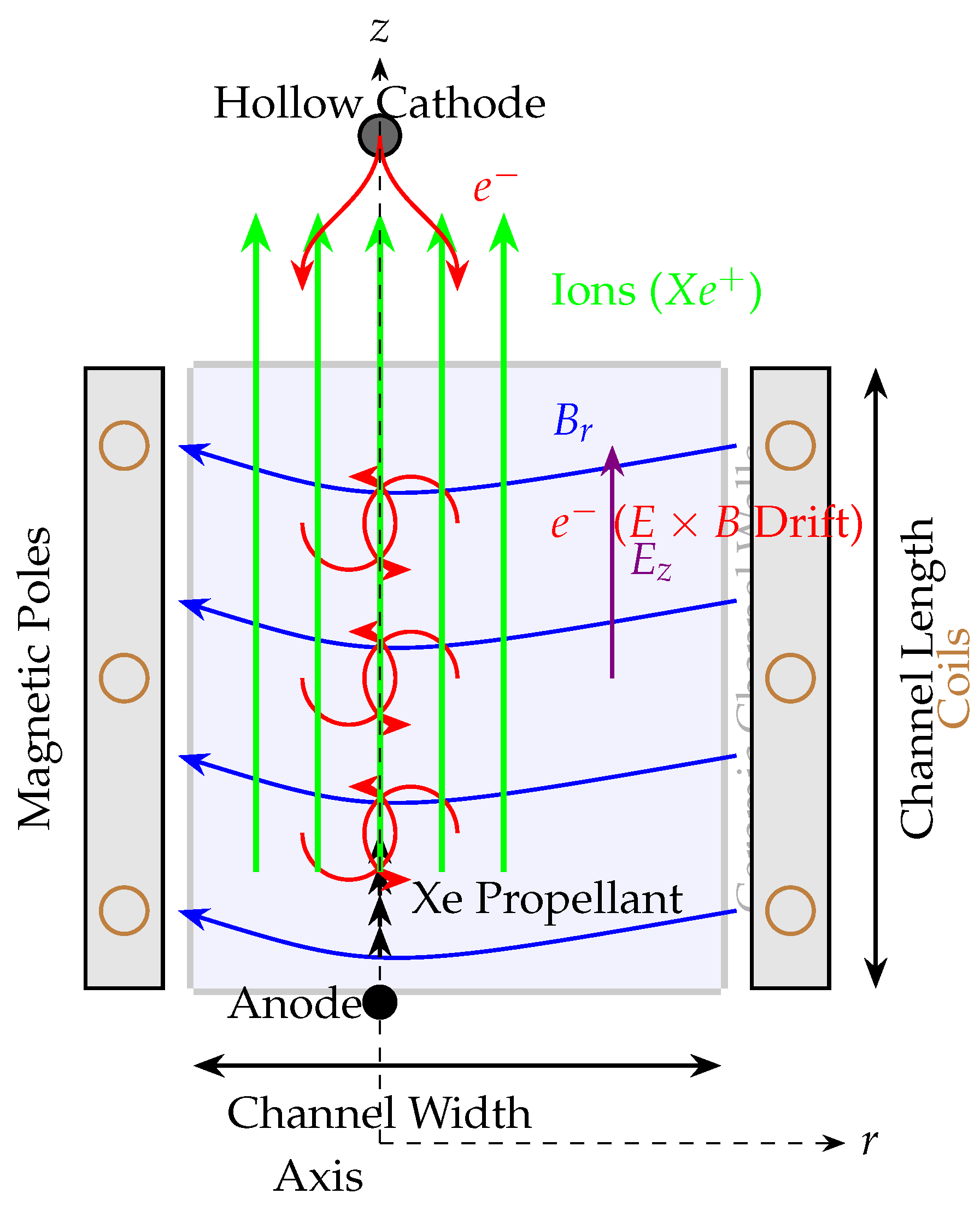
Figure 3.
Cross-helicity in for a representative aligned-flow configuration. (a) Regions where decreases along (growing shear) may correlate with flow disorder. (b) Regions where increases along reflect stronger alignment. Note: is an alignment diagnostic; the thrust criterion itself depends on the motional field (Section 2.3).
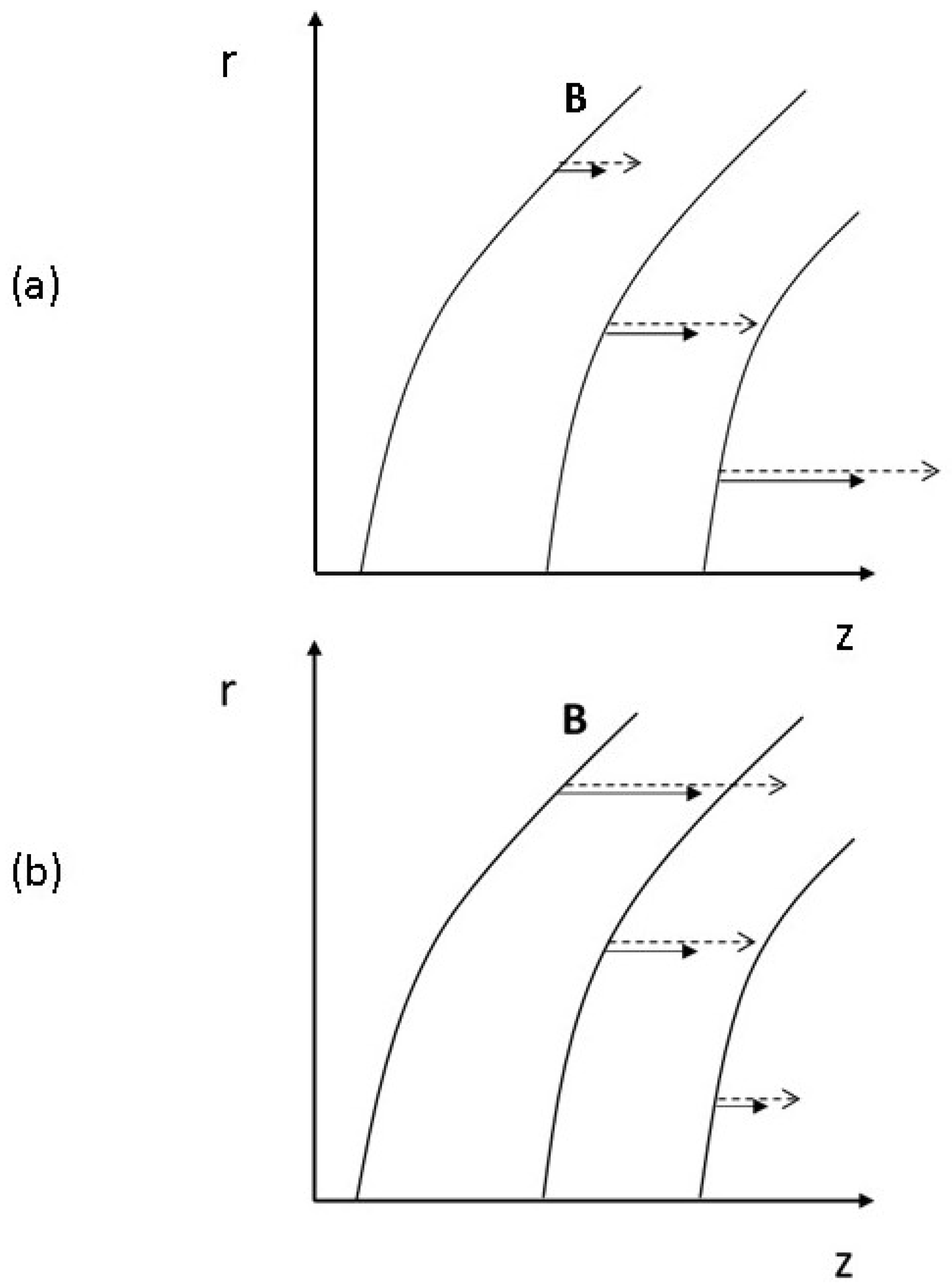
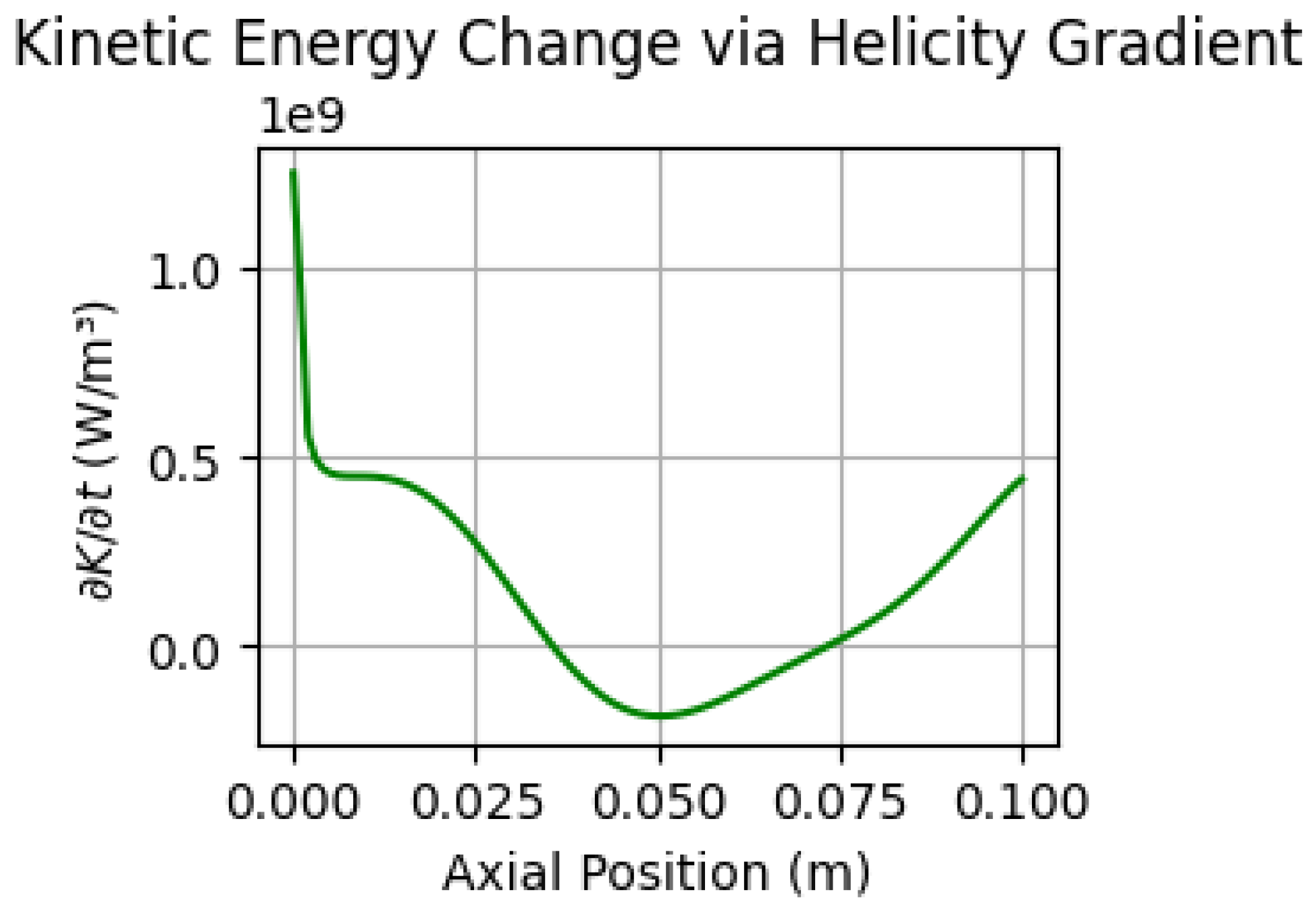
Figure 4.
Axial kinetic-energy rate from the budget in Equation (12). Shaded bands mark regions where ; these coincide with positive mechanical power .
Figure 4.
Axial kinetic-energy rate from the budget in Equation (12). Shaded bands mark regions where ; these coincide with positive mechanical power .
Disclaimer/Publisher’s Note: The statements, opinions and data contained in all publications are solely those of the individual author(s) and contributor(s) and not of MDPI and/or the editor(s). MDPI and/or the editor(s) disclaim responsibility for any injury to people or property resulting from any ideas, methods, instructions or products referred to in the content. |
© 2025 by the authors. Licensee MDPI, Basel, Switzerland. This article is an open access article distributed under the terms and conditions of the Creative Commons Attribution (CC BY) license (http://creativecommons.org/licenses/by/4.0/).
Copyright: This open access article is published under a Creative Commons CC BY 4.0 license, which permit the free download, distribution, and reuse, provided that the author and preprint are cited in any reuse.


