
Submitted:
22 September 2025
Posted:
24 September 2025
You are already at the latest version
Abstract
Neuromorphic hardware systems allow efficient implementation of artificial neural networks (ANNs) across various applications that demand high data throughput, reduced physical size, and low energy consumption. Field-Programmable Gate Arrays (FPGAs) possess inherent features that can be aligned with these requirements. However, implementing ANNs on FPGAs also presents challenges, including the computation of the neuron activation functions, due to the balance between resource constraints and numerical precision. This paper proposes a resource-efficient hardware approximation method for the sigmoid function, utilizing a combination of first- and second-degree polynomial functions. The method aims mainly to reduce approximation error. This paper also evaluates the obtained results against existing techniques and discusses their significance. Experimental results show that the proposed implementation has a good balance between resource usage and approximation error compared to implementations proposed in related works.
Keywords:
neuromorphic hardware
; Field-Programmable Gate Array
; artificial neural network
; neuron activation function
; sigmoid
1. Introduction
The field of neuroengineering is experiencing significant growth, with its activities characterized by several challenging tasks. One important area of focus within this field is the creation of neuromorphic hardware systems. These systems are composed of electronic circuits specifically designed to directly implement artificial neural networks (ANN). The primary aim of developing such systems is to facilitate the application of neural computing models across a broad range of scenarios, each with its unique set of requirements. One critical need addressed by neuromorphic hardware is the acceleration of processing speed in ANN. For instance, many applications require the ability to achieve high data throughput to support fast training and/or recall cycles, such as video processing [1]. Furthermore, some applications require real-time responses from ANN, such as in cryptography/encryption processing [2] and in Internet of Things (IoT) environments, where it is essential to handle data from sensor networks instantly [3]. In addition to processing speed, neuromorphic systems also meet the requirements of mobile applications. For example, robotic platforms can benefit greatly from the reduced physical size and energy consumption of these systems [4]. Additionally, telecommunications is another example of a subject area where minimizing both hardware size and power requirements is important [5]. In this context, neuromorphic systems generally make it feasible to deploy neural network capabilities in compact and energy-efficient devices.
ASIC (Application Specific Integrated Circuit) and FPGA (Field-Programmable Gate Array) technologies allow the creation of highly parallel computing architectures when implementing ANNs, which can achieve greater processing speeds than traditional Central Processing Unit (CPUs) [3]. In addition, the low energy consumption of ASIC and FPGA circuits makes them well-suited for developing embedded neuromorphic systems, offering an advantage over Graphics Processing Unit (GPUs) and CPUs in this regard [6]. While ASIC chips are ideal for ultra-low power applications like brain-computer interfaces, FPGA technology is beneficial due to its shorter development cycles and lower costs for small- and medium-scale production [7]. FPGAs can thus achieve high data throughput while minimizing space and energy use, making them a suitable choice for the types of ANN applications described above.
However, implementing ANNs directly on hardware, particularly on FPGA, also presents several challenges. These difficulties arise from the inherent complexity of neural computations and the constraints of hardware resources. Some of these difficulties include the limited capacity of the chips and the numerical precision of calculations. The challenge of limited hardware resources is related to FPGAs having a finite number of logic blocks (commonly measured in LUTs — Look-Up Tables), memory, and Digital Signal Processing units (DSPs), which can restrict the size and complexity of the networks that can be implemented [8]. The second challenge involves numerical precision, as implementing ANNs on hardware often uses fixed-point arithmetic instead of floating-point [9]. While this strategy saves resources, it can lead to precision loss. Therefore, numerical precision should be monitored in ANN hardware implementations to ensure it does not affect model accuracy. One specific computation in which chip resources and precision issues can arise is in the implementation of neural activation functions like the sigmoid function [10]. The sigmoid function, , is defined as follows:
where represents the slope of the curve and represents the horizontal translation that adjusts the location of the curve’s inflection point. As a neural activation function, the sigmoid function is often used with and [11].
Directly implementing the sigmoid function in hardware is impractical due to the extensive operations involved, such as exponentiation and division. In this way, the present work focuses on developing a hardware-based approximation of the sigmoid function using a combination of first- and second-degree polynomial functions. Based on the outlined motivation, the proposal is intended to be resource-efficient to conserve chip area and maintain numerical precision comparable to previous publications.
A methodological challenge encountered in works related to FPGA algorithm implementations is the wide variety of devices, with different types of internal hardware modules available, produced by different companies, each with its own synthesis software. This often makes direct comparisons between published results produced in different studies impractical. The representation of operands and coefficients used in calculations also varies from study to study, in terms of the total number of bits, the number of bits in the integer part, and the number of bits in the fractional part (when using fixed point representation), potentially rendering comparisons meaningless.
The main contributions of this work are:
- In the sigmoid approximation, it systematically searches for the best boundaries between approximation regions in its domain, rather than establishing them arbitrarily.
- It relaxes the common restriction on using operands that are powers of two, allowing them to assume values freely.
- As a methodological contribution, the results are validated for multiple chip models, from two large companies, making the comparisons with other works fair and more general.
- Also seeking fairness and a methodologically correct procedure, we advocate that the comparison with the results of related works be made by standardizing the number of bits of the operands, the FPGA synthesis programs, and the chip models for implementation.
The remainder of the paper is organized as follows: The next section presents the justification for the study and a review of the literature. Section 3 details the proposed method, and the final two sections present the results, discussion, comparisons to published works, and conclusions.
2. Justification and Related Works
In the field of machine learning, the sigmoid function is a widely used nonlinear component, commonly serving as a neural activation function. It is frequently employed in shallow networks, such as Multilayer Perceptrons (MLP), both during the operation phase (inference) and the training phase, in the derivative for error backpropagation and weight adjustment [11]. However, the sigmoid function is also essential in various other neural computing models beyond MLP. For example, it regulates the retention, forgetting, and passing of information in recurrent neural networks, acting as the activation function for different gates in Long Short-Term Memory (LSTM) networks [12], and in Gated Recurrent Units (GRUs) [13,14]. While the Rectified Linear Unit (ReLU) and its variants, collectively known as the ReLU family, have gained popularity as activation functions in deep learning networks [15], the sigmoid function remains in use within deep models as well. Examples of its use can be found for modulating the flow of information in Structured Attention Networks (SANs), which incorporate structured attention mechanisms to focus on specific parts of the input data [16]. The sigmoid function is also employed to map internal values to a range between 0 and 1 in deep models, particularly for binary decisions or probabilistic outputs, as seen in convolutional neural networks, like LeNet [17], and in Autoencoders [18].
The continued interest in researching the sigmoid function is also reflected in the numerous studies published on its hardware implementation. Common approaches to implementing the sigmoid function include piecewise approximation with linear or non-linear segments, LUTs for direct storage of output values, Taylor series expansion, and Coordinate Rotation Digital Computer (CORDIC) methods. The work [19] aims to achieve low maximum approximation error using CORDIC-based techniques to iteratively calculate trigonometric and hyperbolic functions. However, this approach demands significant chip resources. Similarly, [20] employs Taylor’s theorem and the Lagrange form for approximation. The work also proposes incorporating the reutilization of neuron circuitry into the approximation calculation to enhance chip area efficiency.
For piecewise approximation of the sigmoid curve, [21] utilizes exponential function approximation, which involves complex division operations. A number of studies propose multiple approximation schemes. For instance, [22] introduces an approach using three independent modules — Piecewise Linear Function (PWL), Taylor series, and the Newton-Raphson method — that can be combined to achieve the desired balance between accuracy and resource efficiency. The study in [23] presents two methods for approximation: one centralized and the other distributed, using reconfigurable computing environments to optimize implementation.
Meanwhile, [24] proposes different schemes for sigmoid approximation, utilizing first or second-order polynomial functions depending on the required accuracy and resource usage. Nevertheless, most works focus on different PWL approximation strategies. Reference [25] uses curvature analysis to segment the sigmoid function for PWL approximation, adjusting each segment based on maximum and average error metrics to balance precision and resource consumption. Another approach, [26] employs a first-order Taylor series expansion to define the intersection points of the PWL segments, while [27] leverages statistical probability distribution to determine the number of segments, fragmenting the function into unequal spaces to minimize approximation error. Other approaches aim to reduce computational complexity. For example, [28] explores a technique that combines base-2 logarithmic functions with bit-shift operations for approximation, resulting in reduced chip area.
The use of LUTs for direct storage of sigmoid output values is explored in [29] providing a straightforward method for FPGA implementation. On the other hand, [30] achieves high precision by using floating-point arithmetic, directly computing the sigmoid function with exponent function interpolation via the McLaurin series and Padé polynomials. However, this implementation requires a large chip area.
A restriction adopted in several related works ([22,24,31,32,33]) was to only use multiplications by powers of 2 or operations with base-2 logarithm instead of using coefficients with generic values, in order to use shifts replacing normal multiplications, to save hardware resources. However, this risks sacrificing accuracy.
3. Materials and Methods
As in some of the related works, the scheme proposed here consists in splitting the sigmoid function domain in a small number of subdomains (Figure 1) and in approximating the function in each subdomain by a low-degree polynomial, expecting in this way a low hardware resource usage. The polynomial degrees are chosen based in the function graph form in each subdomain. For x in the function domain, if , will be approximated as being a constant equal to zero. For , will be approximated as being the constant one. For and for , will be approximated by first degree polynomials. For and for , will be approximated by second degree polynomials. However, unlike those works, the boundaries between the approximation regions will not be defined arbitrarily, but will be systematically sought, in an approximately continuous way, in order to minimize the average absolute error in the range . (This range to be explored was chosen here, as in [25], because outside it, is approximately constant, 0 or 1.) As an alternative, the structure of the same algorithm will search for the boundaries that minimizes the maximum (the peak) of the absolute error in the same domain.
Algorithm 1 was used to search for the best approximations boundaries. It was implemented in the GNU Octave software [34]. Initially, the search step dx is set to 0.005. Due to the sigmoid function symmetry about the point , xmed is set to 0. Variables minAvgAbsError and minMaxAbsError are used to register the smaller average absolute error and smaller maximum absolute error, respectively, known up to each iteration along the whole domain. Then, two nested for loops generate many combinations of values to xinf and xmin. (The particular ranges used in those for loops in Algorithm 1 were chosen after experimentation with wider ranges and with larger steps, in a preliminar coarse experiment. Those ranges are used in a final refinement.) In lines 7 and 8, symmetric values about the origin are set for xmax and xsup in relation to xmin and xinf, respectively. Lines from 9 to 14 build sequences of values for x in each of the approximations regions. Lines 15 to 20 build sequences containing the standard values for the sigmoid in each region. In lines from 21 to 24, the Octave function polyfit is applied to the sequences belonging to each of the regions where polynomial approximations are adopted, using the least square error criterion. (The third polyfit argument is the degree of the desired polynomial.) Variables , , and receive the polynomials coefficients of the corresponding regions. Lines from 25 to 31 calculate and concatenate the errors for each domain value. Line 32 calculates the average absolute error (avgAbsError) and line 33 calculates the maximum absolute error (maxAbsError) for the current combination. Lines 34 to 42 check if the newly calculated avgAbsError is smaller than the least average absolute error known up to this moment, case in which the corresponding optimal conditions are registered. The same kind of checking is performed for maxAbsError in lines from 43 to 51. So, at the execution end, the best boundaries and the corresponding polynomials coefficients are known for both criteria. There was no concern about optimizing this algorithm in terms of execution time, because it only needs to be executed once. We do not adopt here the restriction or preference for operations involving powers of 2, thus leaving the possibilities of values for the polynomial coefficients and for the boundaries more free.
The application of Algorithm 1 to any other function (for example the hyperbolic tangent, also a common neural activation function [11]) is straightforward. It will suffice to replace the sigmoid calculation in lines from 15 to 20 by that function. Depending on that function characteristics, one may change the number of regions in the domain and the polynomial degrees, but the strategy remains the same.
The results obtained by Algorithm 1 are shown in Table 1.
Table 1 shows that, as expected, the average absolute error was slightly lower in the first implementation than in the second. The maximum absolute error was slightly lower in the second implementation than in the first.
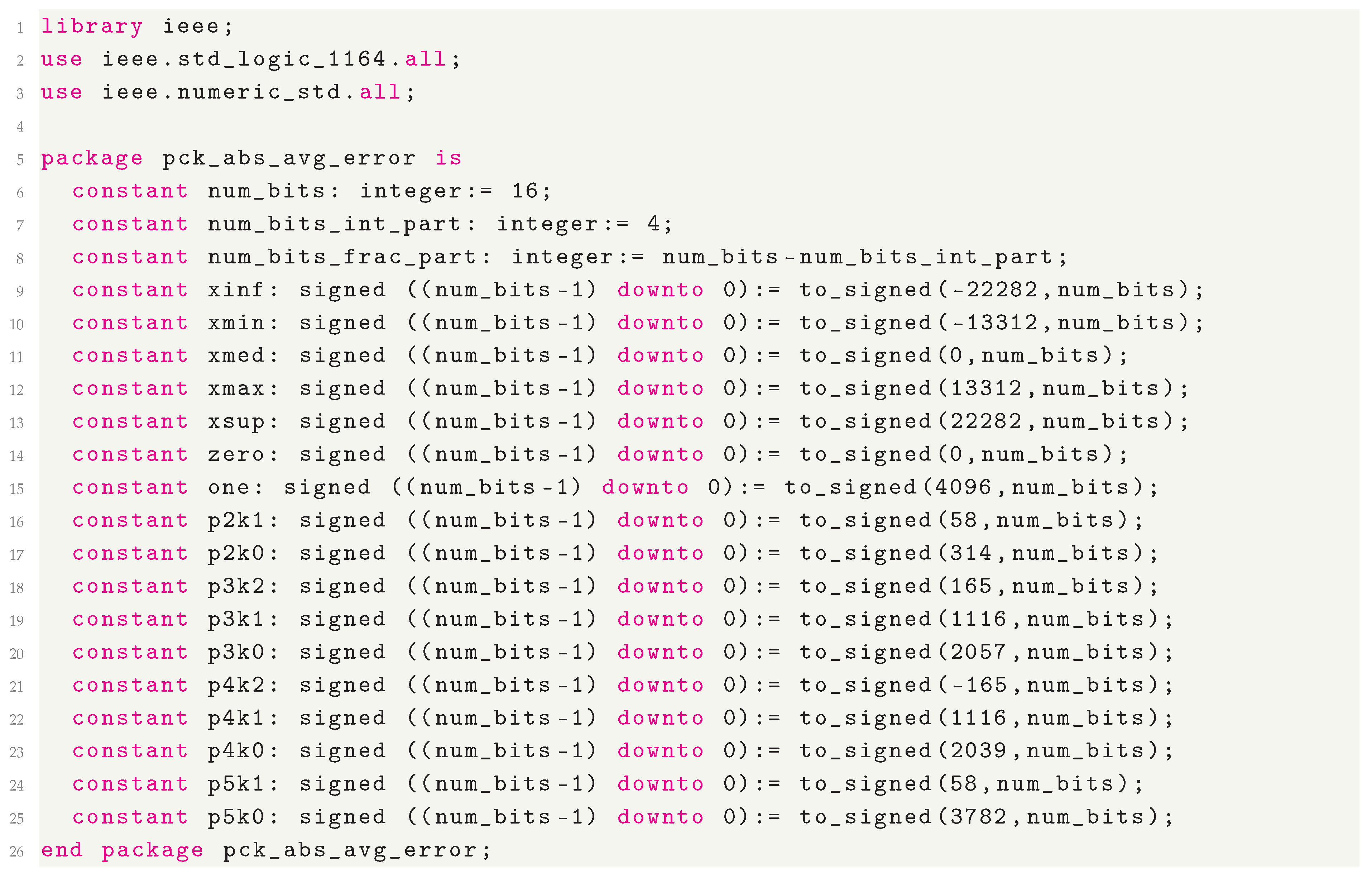
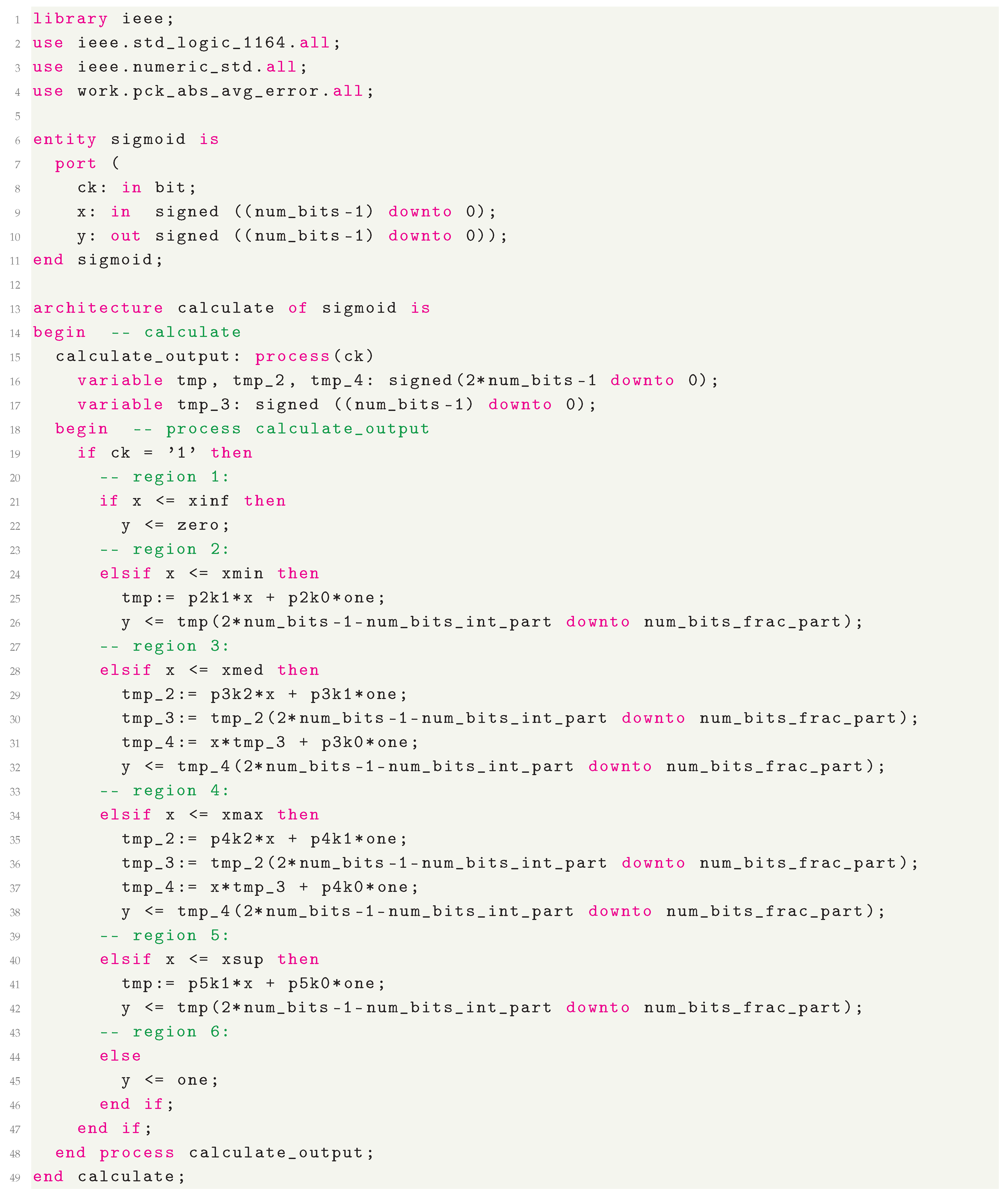
The two sigmoid modules corresponding to Table 1 were implemented in Very High Speed Integrated Circuits Hardware Description Language (VHDL) language [35], in a behavioral way. Each implementation consists in two VHDL files: a package file, called pck_abs_avg_error.vhdl (in Appendix A.1) when containing constants definitions for the first module) and a sigmoid.vhdl file (in Appendix A.2), containing the approximation algorithm. Those constants are the polynomial coefficients and the boundaries values. The package file for the second module are omitted here because only the constant values change between the two implementations. The sigmoid.vhdl file is the same for both.
| Algorithm 1 Search for the best boundaries between approximation regions |
|
The input x, the output , the boundaries values and the polynomial coefficients are all represented as 16 bit numbers, in fixed point, with 4 bits for the integer part and 12 bits for the fractional part, as in [25]. So the real number 1 is represented as the binary number , which corresponds to the decimal number (without considering the decimal point position). Thus each constant in Table 1 appears multiplied by 4096 in the VHDL file pck_abs_avg_error.vhdl. Two’s complement representation was used to allow calculations with negative numbers, by using the type signed from the ieee.numeric_std VHDL package.
The sigmoid implementation in the file sigmoid.vhdl follows directly from Table 1 and from Figure 1. An x value is read at the clock (ck) rise and the output y is then calculated according to the x approximation region. After each multiplication operation is performed, its result contains a number of bits that is the sum of the numbers of bits of its operands: 8 bits to the integer part and 24 bits to the fractional part. So, following this operation, the result is truncated, by discarding the 4 leftmost and the 12 rightmost bits, producing a number respecting again the convention with 16 bits. Due to the multiplication operands particular values used here (Table 1), the resulting 4 leftmost bits are always zeros for positive results and ones for negative results (in two’s complement), allowing them to be discarded. Discarding the 12 least significant bits affects the results very little, because they have very small weights.
To compare the hardware resources usage and accuracy of our implementations with those of related works cited in Section 2, we attempted to reimplement them all in a uniform way, not necessarily identical to theirs, but seeking to reproduce as faithfully as possible their algorithms and their sigmoid approximations, by using a uniform fixed-point representation, with the same number of bits (16 bits, being 4 bits for the integer part and 12 bits for the decimal part), on uniform chip models, and using uniform synthesis programs. This was possible only for some of the related works, [22,24,25,31,32,33], because their implementations were described in sufficient detail there. Each proposed sigmoid approximation was described in VHDL. The synthesis programs were Quartus Prime Version 24.1 std, Build 1077 SC Lite Edition, for the FPGA chips Device 5CGXFC7C7F23C8 and Device MAX-10 10M02DCU324A6G, and Vivado v2025.1, for the FPGA chips Virtex-7 - Device xc7v585tffg1157-3, Spartan-7 - Device xc7s75fgga484-1 and Zinq-7000 - Device xc7z045iffg900-2L. So, programs were chosen from companies that are among the leaders in the FPGA field and, for each company, chips of varying levels of complexity were chosen.
Regarding accuracy, the criterion most used in the cited works was the average absolute error of the function over the domain considered, which justifies its adoption here.
Each VHDL description used in the comparisons was simulated using the GHDL program [36], because it is fast to execute and is capable of recording results in text files for later analysis. Each simulation run consisted in calculating and comparing the standard value of the sigmoid function, , with the value generated by the system described in VHDL, for each of the possible values in the x domain and obtaining, at the end, the average of the absolute error.
4. Results
Table 2 shows the synthesis results regarding the use of hardware resources in the FPGA, for each sigmoid approximation. There are six approximations from related works and our two approximations: to minimize the error average (“ours avg.”) and to minimize the maximum error (“ours max.”). The table has five parts, one for each software-device combination. It shows the FPGA resources used by each implementation as reported by the corresponding synthesis software. The kinds of those resources vary depending on the device type. For instance, only some devices have DSP blocks. The last column shows the total available number of each resource type in each FPGA device. The percentage of usage of each resource type relative to availability is also indicated. Reports from all implementations indicated that 16 registers (due to 16-bit operands) and 33 pins (16 input bits, 16 output bits, and a clock pin) were used. Thus, these results were omitted from Table 2, keeping in it only those relevant for comparison purposes.
Comparing resources usage between implementations is not straightforward because they are of different types and available in different quantities. But, at first glance, one can see in Table 2 that our implementations are neither systematically better nor systematically worse, in general, than the others in terms of resource usage, even though this criterion did not guide the creation of our implementations. Specifically, only implementation [31] always matches ours or is advantageous.
Table 3 shows the average absolute error for all sigmoid implementations, obtained for 65536 equally spaced values in its domain. It should be noted that, instead of Table 2, these results do not depend on the chip model on which the implementation was made, but only on the VHDL descriptions.
In Table 3, one can see that only implementation [22] managed to achieve a lower error than ours. But in Table 2, we see that it used more resources of most types compared to our implementations. Another interesting result was that our second implementation, which aimed only to obtain the minimum error peak, surpassed almost all others in the average absolute error criterion. The implementation [31], which is advantageous compared to ours concerning resources usage, has a much bigger average absolute error.
The absolute error for our first implementation is shown in Figure 2 and for the second implementation in Figure 3 for the function domain.
The maximum absolute errors of our implementations were 0.0068181 for the first and 0.0071184 for the second. They are larger than before VHDL implementations occur (Table 1), surely due to the use of fixed point representation in 16 bits. Another effect was that now, the maximum error of the first implementation is lower than that of the second implementation. But, in some cases, the second implementation is advantageous in relation to the first in resources utilization (Table 2).
5. Discussion
The sigmoid approximation for its implementation in FPGA, by dividing its domain into a few subdomains, approximating it, in each subdomain, using a low-degree polynomial and systematically searching for the best boundaries between the subdomains allowed us to obtain results with a good compromise between the use of hardware resources and the average absolute approximation error. It thus becomes a good alternative to preexisting solutions.
The fact that we did not restrict operands or boundaries between approximation regions to be powers of two did not prevent relatively good results from being obtained not only in error value, but also in resource usage. Therefore, consideration should be given to the use of such restrictions.
The method proposed here aimed to obtain a low value for the average absolute error. In this, [22] obtained a better result, using a more elaborate method, including Newton-Raphson approximation, but requiring greater use of hardware resources in most cases. Therefore, it may be preferred when the importance of the error is much greater than the importance of the use of resources.
A limitation of this work was that it attempted to reproduce the implementations described in other studies, with the possibility that this reproduction might have had differences from the originals that could have influenced the results. Furthermore, some of those proposals allowed for parameter adjustments, whereas in this reproduction, to minimize the length of the work, we sought to use only a typical version of what was described in each article.
As future work, a complete neural network can be implemented in FPGA using, in each neuron, a sigmoid implementation as proposed here, comparing its performance with a version implemented in a general-purpose computer.
One can also investigate the implementation of other activation functions, such as the hyperbolic tangent, using the principles used here for the sigmoid.
Author Contributions
Conceptualization, M.A.A.S., S.D.S. and R.P.; methodology, all the authors; software, all the authors; validation, all the authors; formal analysis, M.A.A.S., S.D.S. and R.P.; investigation, all the authors; resources, all the authors; data curation, all the authors; writing—original draft preparation, all the authors; writing—review and editing, all the authors; visualization, all the authors; supervision, M.A.A.S., S.D.S. and R.P.; project administration, M.A.A.S., S.D.S. and R.P.; funding acquisition, M.A.A.S., S.D.S.. All authors have read and agreed to the published version of the manuscript.
Funding
This research was funded by Conselho Nacional de Desenvolvimento Científico e Tecnológico (CNPq), which provided a research grant to author V.A.B., and by Instituto Federal de Educação, Ciência e Tecnologia de São Paulo, which provided a research grant to author R.M.N.
Data Availability Statement
The VHDL and Octave code used in the study are openly available in https://github.com/AngeloIFSP/FPGA-implementation-of-sigmoid-approximation-for-neural-networks
Conflicts of Interest
The authors declare no conflicts of interest.
Abbreviations
The following abbreviations are used in this manuscript:
| ANN | artificial neural network |
| ASIC | Application Specific Integrated Circuit |
| CORDIC | Coordinate Rotation Digital Computer |
| CPU | Central Processing Unit |
| DSP | Digital Signal Processing |
| FPGA | Field-Programmable Gate Arrays |
| GPU | Graphics Processing Unit |
| GRU | Gated Recurrent Units |
| LSTM | Long Short-Term Memory |
| LUT | Look-Up Table |
| MLP | Multilayer Perceptron |
| PWL | Piecewise Linear Function |
| ReLU | Rectified Linear Unit |
| SAN | Structured Attention Network |
| VHDL | Very High Speed Integrated Circuits Hardware Description Language |
Appendix A. VHDL Source Code
Appendix A.1. Package containing definitions, minimizing average absolute error version
Appendix A.2. Sigmoid implementation
References
- de Sousa, M.A.d.A.; Pires, R.; Del-Moral-Hernandez, E. SOMprocessor: A high throughput FPGA-based architecture for implementing Self-Organizing Maps and its application to video processing. Neural Networks 2020, 125, 349–362. [Google Scholar] [CrossRef] [PubMed]
- Teodoro, A.A.; Gomes, O.S.; Saadi, M.; Silva, B.A.; Rosa, R.L.; Rodríguez, D.Z. An FPGA-based performance evaluation of artificial neural network architecture algorithm for IoT. Wireless Personal Communications 2022, 127, 1085–1116. [Google Scholar] [CrossRef]
- Qian, B.; Su, J.; Wen, Z.; Jha, D.N.; Li, Y.; Guan, Y.; Puthal, D.; James, P.; Yang, R.; Zomaya, A.Y.; et al. Orchestrating the development lifecycle of machine learning-based IoT applications: A taxonomy and survey. ACM Computing Surveys (CSUR) 2020, 53, 1–47. [Google Scholar] [CrossRef]
- Korayem, M.H.; Adriani, H.R.; Lademakhi, N.Y. Regulation of cost function weighting matrices in control of WMR using MLP neural networks. Robotica 2023, 41, 530–547. [Google Scholar] [CrossRef]
- de Abreu de Sousa, M.A.; Pires, R.; Del-Moral-Hernandez, E. OFDM symbol identification by an unsupervised learning system under dynamically changing channel effects. Neural Computing and Applications 2018, 30, 3759–3771. [Google Scholar] [CrossRef]
- Dundar, A.; Jin, J.; Martini, B.; Culurciello, E. Embedded streaming deep neural networks accelerator with applications. IEEE transactions on neural networks and learning systems 2016, 28, 1572–1583. [Google Scholar] [CrossRef]
- Nurvitadhi, E.; Sheffield, D.; Sim, J.; Mishra, A.; Venkatesh, G.; Marr, D. Accelerating binarized neural networks: Comparison of FPGA, CPU, GPU, and ASIC. In Proceedings of the 2016 International Conference on Field-Programmable Technology (FPT); IEEE, 2016; pp. 77–84. [Google Scholar]
- Mittal, S. A survey of FPGA-based accelerators for convolutional neural networks. Neural computing and applications 2020, 32, 1109–1139. [Google Scholar] [CrossRef]
- Tao, Y.; Ma, R.; Shyu, M.L.; Chen, S.C. Challenges in energy-efficient deep neural network training with FPGA. In Proceedings of the IEEE/CVF conference on computer vision and pattern recognition workshops; 2020; pp. 400–401. [Google Scholar]
- Tisan, A.; Oniga, S.; Mic, D.; Buchman, A. Digital implementation of the sigmoid function for FPGA circuits. Acta Technica Napocensis Electronics and Telecommunications 2009, 50, 6. [Google Scholar]
- Haykin, S.S. Neural networks and learning machines, 3rd ed.; Pearson Education: Upper Saddle River, NJ, 2009. [Google Scholar]
- Moharm, K.; Eltahan, M.; Elsaadany, E. Wind speed forecast using LSTM and Bi-LSTM algorithms over gabal El-Zayt wind farm. In Proceedings of the 2020 International Conference on Smart Grids and Energy Systems (SGES); IEEE, 2020; pp. 922–927. [Google Scholar]
- Dey, R.; Salem, F.M. Gate-variants of gated recurrent unit (GRU) neural networks. In Proceedings of the 2017 IEEE 60th international midwest symposium on circuits and systems (MWSCAS); IEEE, 2017; pp. 1597–1600. [Google Scholar]
- Gharehbaghi, A.; Ghasemlounia, R.; Ahmadi, F.; Albaji, M. Groundwater level prediction with meteorologically sensitive Gated Recurrent Unit (GRU) neural networks. Journal of Hydrology 2022, 612, 128262. [Google Scholar] [CrossRef]
- Nair, V.; Hinton, G.E. Rectified linear units improve restricted boltzmann machines. In Proceedings of the 27th international conference on machine learning (ICML-10); 2010; pp. 807–814. [Google Scholar]
- Yang, L.; Han, J.; Zhao, T.; Liu, N.; Zhang, D. Structured attention composition for temporal action localization. arXiv 2022, arXiv:2205.09956. [Google Scholar] [CrossRef] [PubMed]
- Li, L.; Wang, Y. Improved LeNet-5 convolutional neural network traffic sign recognition [J]. International core journal of engineering 2021, 7, 114–121. [Google Scholar]
- Sewak, M.; Sahay, S.K.; Rathore, H. An overview of deep learning architecture of deep neural networks and autoencoders. Journal of Computational and Theoretical Nanoscience 2020, 17, 182–188. [Google Scholar] [CrossRef]
- Tiwari, V.; Khare, N. Hardware implementation of neural network with Sigmoidal activation functions using CORDIC. Microprocessors and Microsystems 2015, 39, 373–381. [Google Scholar] [CrossRef]
- Del Campo, I.; Finker, R.; Echanobe, J.; Basterretxea, K. Controlled accuracy approximation of sigmoid function for efficient FPGA-based implementation of artificial neurons. Electronics Letters 2013, 49, 1598–1600. [Google Scholar] [CrossRef]
- Gomar, S.; Mirhassani, M.; Ahmadi, M. Precise digital implementations of hyperbolic tanh and sigmoid function. In Proceedings of the 2016 50th Asilomar Conference on Signals, Systems and Computers; IEEE, 2016; pp. 1586–1589. [Google Scholar]
- Pan, Z.; Gu, Z.; Jiang, X.; Zhu, G.; Ma, D. A modular approximation methodology for efficient fixed-point hardware implementation of the sigmoid function. IEEE Transactions on Industrial Electronics 2022, 69, 10694–10703. [Google Scholar] [CrossRef]
- Shatravin, V.; Shashev, D.; Shidlovskiy, S. Sigmoid activation implementation for neural networks hardware accelerators based on reconfigurable computing environments for low-power intelligent systems. Applied Sciences 2022, 12, 5216. [Google Scholar] [CrossRef]
- Vassiliadis, S.; Zhang, M.; Delgado-Frias, J.G. Elementary function generators for neural-network emulators. IEEE transactions on neural networks 2000, 11, 1438–1449. [Google Scholar] [PubMed]
- Li, Z.; Zhang, Y.; Sui, B.; Xing, Z.; Wang, Q. FPGA implementation for the sigmoid with piecewise linear fitting method based on curvature analysis. Electronics 2022, 11, 1365. [Google Scholar] [CrossRef]
- Qin, Z.; Qiu, Y.; Sun, H.; Lu, Z.; Wang, Z.; Shen, Q.; Pan, H. A novel approximation methodology and its efficient vlsi implementation for the sigmoid function. IEEE Transactions on Circuits and Systems II: Express Briefs 2020, 67, 3422–3426. [Google Scholar] [CrossRef]
- Wei, L.; Cai, J.; Nguyen, V.; Chu, J.; Wen, K. P-SFA: Probability based sigmoid function approximation for low-complexity hardware implementation. Microprocessors and Microsystems 2020, 76, 103105. [Google Scholar] [CrossRef]
- Zaki, P.W.; Hashem, A.M.; Fahim, E.A.; Mansour, M.A.; ElGenk, S.M.; Mashaly, M.; Ismail, S.M. A novel sigmoid function approximation suitable for neural networks on FPGA. In Proceedings of the 2019 15th International Computer Engineering Conference (ICENCO); IEEE, 2019; pp. 95–99. [Google Scholar]
- Pogiri, R.; Ari, S.; Mahapatra, K. Design and FPGA Implementation of the LUT based Sigmoid Function for DNN Applications. In Proceedings of the 2022 IEEE International Symposium on Smart Electronic Systems (iSES); IEEE, 2022; pp. 410–413. [Google Scholar]
- Hajduk, Z. Hardware implementation of hyperbolic tangent and sigmoid activation functions. Bulletin of the Polish Academy of Sciences. Technical Sciences 2018, 66, 563–577. [Google Scholar] [CrossRef]
- Liu, F.; Zhang, B.; Chen, G.; Gong, G.; Lu, H.; Li, W. A novel configurable high-precision and low-cost circuit design of sigmoid and tanh activation function. In Proceedings of the 2021 IEEE International Conference on Integrated Circuits, Technologies and Applications (ICTA); IEEE, 2021; pp. 222–223. [Google Scholar]
- Tsmots, I.; Skorokhoda, O.; Rabyk, V. Hardware implementation of sigmoid activation functions using FPGA. In Proceedings of the 2019 IEEE 15th International Conference on the Experience of Designing and Application of CAD Systems (CADSM); IEEE, 2019; pp. 34–38. [Google Scholar]
- Vaisnav, A.; Ashok, S.; Vinaykumar, S.; Thilagavathy, R. FPGA implementation and comparison of sigmoid and hyperbolic tangent activation functions in an artificial neural network. In Proceedings of the 2022 International Conference on Electrical, Computer and Energy Technologies (ICECET); IEEE, 2022; pp. 1–4. [Google Scholar]
- Eaton, J.W.; Bateman, D.; Hauberg, S.; Wehbring, R. GNU Octave version 4.4.0 manual: a high-level interactive language for numerical computations, 2018.
- Ashenden, P. The Designer’s Guide to VHDL; Morgan Kauffman Publishers, 2008.
- Gingold, T. GHDL, 2017. Available at http://ghdl.free.fr/.
Figure 1.
Ranges for approximations in the sigmoid domain. The boundaries are drawn in approximate positions, to be defined by an algorithm to be described below.
Figure 1.
Ranges for approximations in the sigmoid domain. The boundaries are drawn in approximate positions, to be defined by an algorithm to be described below.
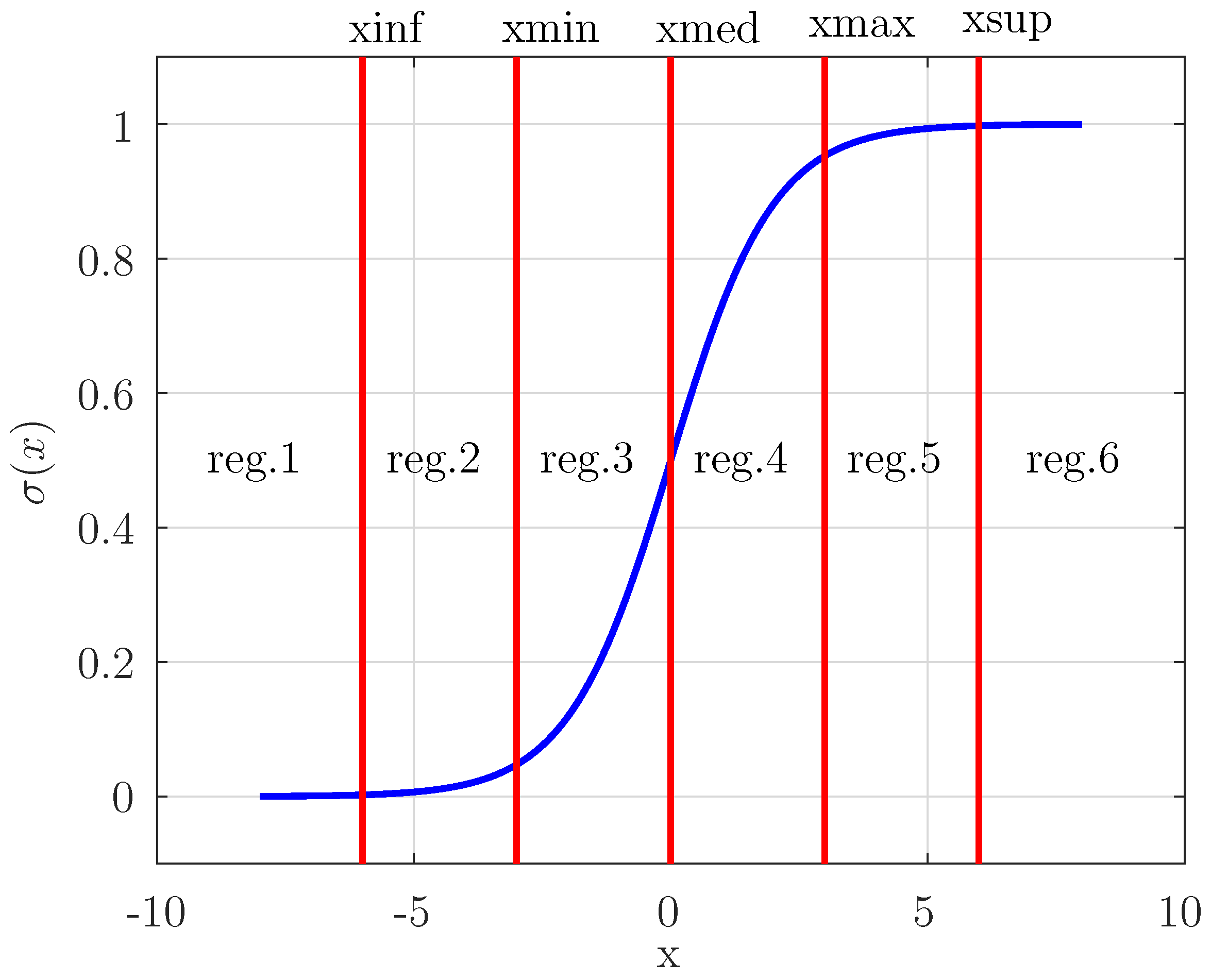
Figure 2.
Absolute error for our first implementation.
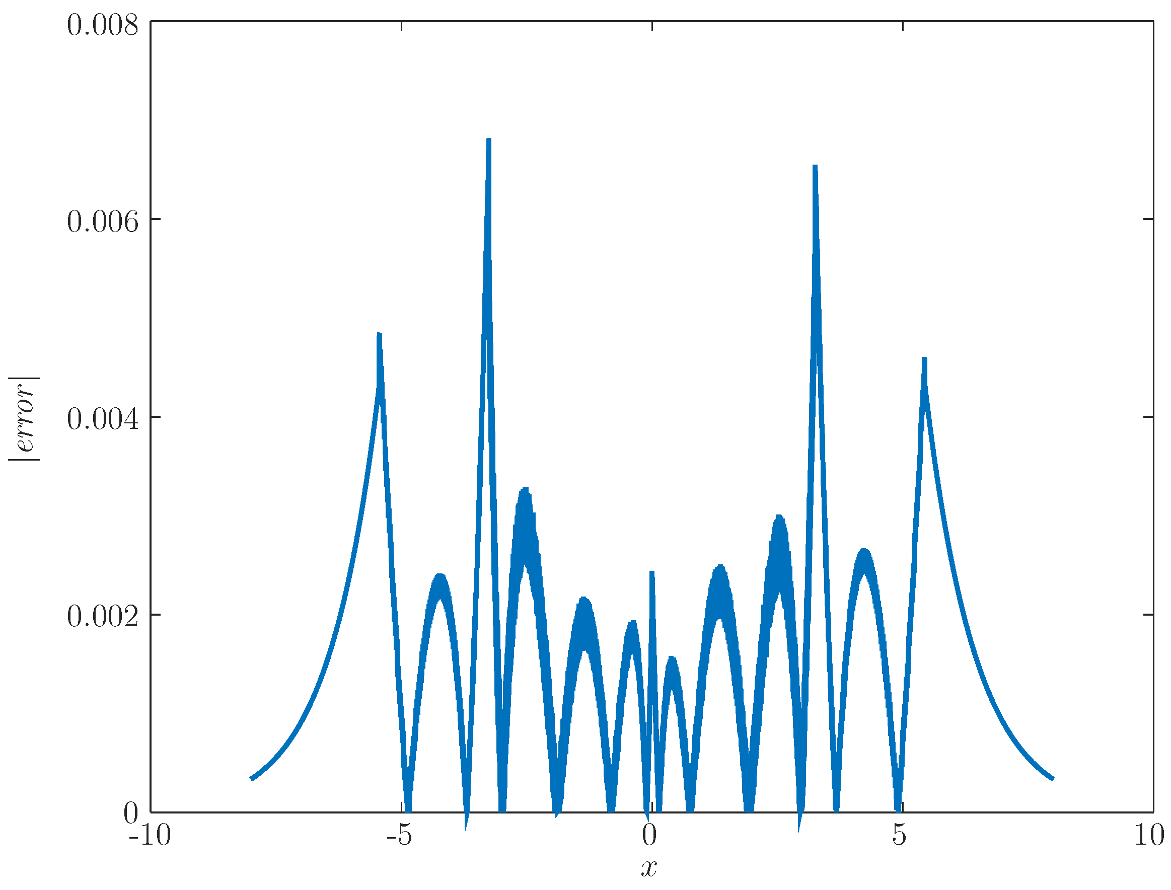
Figure 3.
Absolute error for our second implementation.
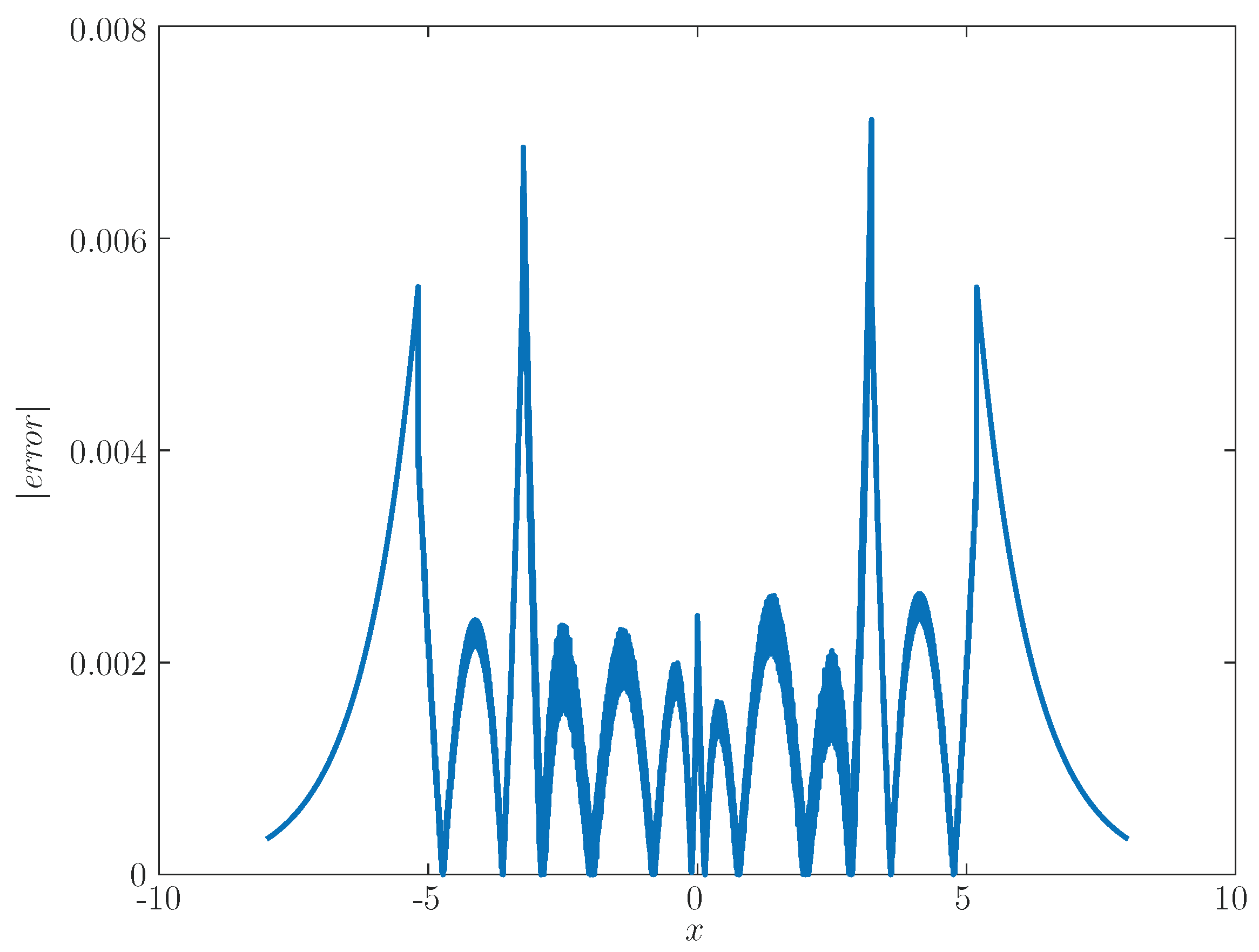

Table 1.
Results obtained by Algorithm 1.
| To obtain the minimal average absolute error: | |
| minAvgAbsError | 0.0016548 |
| minMaxAbsError | 0.0064729 |
| region 2 polynomial | |
| region 3 polynomial | |
| region 4 polynomial | |
| region 5 polynomial | |
| To obtain the minimal maximum absolute error: | |
| minAvgAbsError | 0.0016775 |
| minMaxAbsError | 0.0055832 |
| region 2 polynomial | |
| region 3 polynomial | |
| region 4 polynomial | |
| region 5 polynomial | |
Table 2.
Results on FPGA used resources. (Only results that varied between implementations are shown.)
Table 2.
Results on FPGA used resources. (Only results that varied between implementations are shown.)
| Quartus Prime Version 24.1 std . 0 Build 1077 SC Lite Edition | |||||||||
| Family Ciclone V - Device 5CGXFC7C7F23C8 | |||||||||
| work | [25] | [31] | [22] | [32] | [33] | [24] | ours | ours | avail- |
| avg. | max. | able | |||||||
| Logic Utilization | 117 | 25 | 91 | 39 | 41 | 176 | 25 | 52 | 56480 |
| percentage | 0.21 | 0.04 | 0.16 | 0.07 | 0.07 | 0.31 | 0.04 | 0.09 | 100 |
| DSP Blocks | 4 | 2 | 6 | 3 | 0 | 8 | 5 | 4 | 156 |
| percentage | 2.56 | 1.28 | 3.85 | 1.92 | 0.00 | 5.13 | 3.21 | 2.56 | 100 |
| Quartus Prime Version 24.1 std . 0 Build 1077 SC Lite Edition | |||||||||
| Device MAX-10 10M02DCU324A6G | |||||||||
| work | [25] | [31] | [22] | [32] | [33] | [24] | ours | ours | avail- |
| avg. | max. | able | |||||||
| Logic Elements | 505 | 95 | 394 | 238 | 79 | 424 | 362 | 310 | 2304 |
| percentage | 21.92 | 4.12 | 17.10 | 10.33 | 3.43 | 18.40 | 15.71 | 13.45 | 100 |
| Embed. Multiplier | 0 | 4 | 6 | 2 | 0 | 16 | 4 | 4 | 32 |
| percentage | 0.00 | 12.50 | 18.75 | 6.25 | 0.00 | 50.00 | 12.50 | 12.50 | 100 |
| Vivado v2025.1 | |||||||||
| Family Virtex-7 - Device xc7v585tffg1157-3 | |||||||||
| work | [25] | [31] | [22] | [32] | [33] | [24] | ours | ours | avail- |
| avg. | max. | able | |||||||
| LUT as Logic | 202 | 66 | 168 | 86 | 114 | 282 | 67 | 80 | 364200 |
| percentage | 0.06 | 0.02 | 0.05 | 0.02 | 0.03 | 0.08 | 0.02 | 0.02 | 100 |
| DSPs | 4 | 2 | 5 | 3 | 0 | 8 | 6 | 4 | 1260 |
| percentage | 0.32 | 0.16 | 0.40 | 0.24 | 0.00 | 0.63 | 0.48 | 0.32 | 100 |
| Vivado v2025.1 | |||||||||
| Family Spartan-7 - Device xc7s75fgga484-1 | |||||||||
| work | [25] | [31] | [22] | [32] | [33] | [24] | ours | ours | avail- |
| avg. | max. | able | |||||||
| LUT as Logic | 202 | 66 | 169 | 86 | 114 | 281 | 67 | 80 | 48000 |
| percentage | 0.42 | 0.14 | 0.35 | 0.18 | 0.24 | 0.59 | 0.14 | 0.17 | 100 |
| DSPs | 4 | 2 | 5 | 3 | 0 | 8 | 6 | 4 | 140 |
| percentage | 2.86 | 1.43 | 3.57 | 2.14 | 0.00 | 5.71 | 4.29 | 2.86 | 100 |
| Vivado v2025.1 | |||||||||
| Family Zinq-7000 - Device xc7z045iffg900-2L | |||||||||
| work | [25] | [31] | [22] | [32] | [33] | [24] | ours | ours | avail- |
| avg. | max. | able | |||||||
| LUT as Logic | 202 | 66 | 169 | 86 | 114 | 282 | 67 | 80 | 218600 |
| percentage | 0.09 | 0.03 | 0.08 | 0.04 | 0.05 | 0.13 | 0.03 | 0.04 | 100 |
| DSPs | 4 | 2 | 5 | 3 | 0 | 8 | 6 | 4 | 900 |
| percentage | 0.44 | 0.22 | 0.56 | 0.33 | 0.00 | 0.89 | 0.67 | 0.44 | 100 |
Table 3.
Average absolute error in the sigmoid implementation, obtained for 65536 equally spaced values in its domain.
Disclaimer/Publisher’s Note: The statements, opinions and data contained in all publications are solely those of the individual author(s) and contributor(s) and not of MDPI and/or the editor(s). MDPI and/or the editor(s) disclaim responsibility for any injury to people or property resulting from any ideas, methods, instructions or products referred to in the content. |
© 2025 by the authors. Licensee MDPI, Basel, Switzerland. This article is an open access article distributed under the terms and conditions of the Creative Commons Attribution (CC BY) license (http://creativecommons.org/licenses/by/4.0/).
Copyright: This open access article is published under a Creative Commons CC BY 4.0 license, which permit the free download, distribution, and reuse, provided that the author and preprint are cited in any reuse.


