The Role of Gaussian and Mean Curvature in 3-D Highway Geometric Design and Safety

1. Introduction

Highway safety is a major health issue that requires continued efforts for effectively addressing it and developing sustainable preventive solutions. The roadway environment is a difficult and complex system that people have to deal with and is a major contributor to road traffic injuries and fatalities. In 2015, there were 32,166 fatalities and over 1.7 million injuries (NHTSA n.d.). There is a systematic effort to improve roadway design to address these issues and identify roadway design elements that could contribute to designing roadways having the potential to improve safety by creating an environment that drivers can easily understand. The objective of this research is to contribute to the enhancement of road safety through the development of a 3-dimensional (3-D) model for rural highways that would allow for a more accurate correlation of design elements to their potential crash contribution. The road surface will be modeled as a 3-D surface through differential geometry and B-spline surfaces, leading to a more realistic, complete, and accurate representation of the actual roadway geometry that explicitly or implicitly affects the crash occurrence probability.

Current highway safety research has developed crash prediction models that quantify the impact of single geometric elements on crash occurrence. For example, in the Highway Safety Manual (HSM) there are models that predict the effect of lane width, shoulder width, presence of median, etc. on crashes but each of them defines it singularly without considering their potential interactions (AASHTO 2010). The highway safety community has recognized the need to estimate these interactions and the recent approach to address it is to either estimate the contribution of each geometric element on the crash occurrence alone or use a set of crash modification factors to adjust the estimate for a base condition to the existing features estimating their effect through multiplication of these factors (Washington et al. 2010; Hanno 2004). The number of variable interactions can increase exponentially even when a few are considered, e.g. five variables can produce 27 interactions, resulting in a drastically reduced statistical power of the analysis and a higher probability of not producing statistically significant models. Although there are statistical techniques in theory that may address this issue, practically the problem is still apparent and indicates the need for a much more integrated and coherent modeling approach of the roadway elements.

Another issue that is relevant and underscores the importance of this research effort is the fact that to date highway safety research is based on a 2-dimensional (2-D) approach, i.e., horizontal and vertical alignment, whose principles were initially established in the 1940’s and have not drastically changed since then. Over the years, although there have been changes in terms of adjusting minimum values and thresholds of various design elements, the overall methodology regarding highway safety estimation remains intact. Even though the roadway is a 3-D structure, the simplification of its projection in two planes, i.e., horizontal and vertical, has served well in the past when it was adequate to do so. However, given the computational power that is available nowadays one can argue that the geometric design process can be further improved in terms of incorporating a 3-D approach and metrics to express the roadway alignment. Moreover, this approach could be carried forward to safety evaluation and possibly enhance the ability to examine simultaneously the potential contribution of more than a single geometric element on crash occurrence. Today, 3-D geometric interactions are not reported in a quantifiable form in any highway design or safety manual. The coordination between the horizontal and vertical alignment is limited to earthwork estimation or optimization, but not during the design process because the 3-D design incorporation has traditionally been a mathematically and computationally demanding procedure. Therefore, the true extent of the design interactions and implications are not taken into consideration in terms of a holistic 3-D approach (Hassan and Easa 1998a, 2000; Hassan et al. 1996a, 2000; Hanno 2004). Others have noted that improper horizontal and vertical alignment coordination play a crucial role in crash frequency occurrence (Lamm and Smith 1999; Biduka et al. 2002) and could also confuse the driver in terms of selecting an appropriate operating speed (Lamm et al. 1999). Lamm and Choueri (1987) provide a very enlightening description of improper as well as desirable horizontal and vertical combinations that affect the driver’s perception and expectation of the roadway. Easa et al. (1999, 2001, 2002) have also highlighted the horizontal and vertical coordination problem and its implications, which could result in sudden fluctuations in operating speed, and underestimation of horizontal element lengths for sight distance calculation. Moreover, the AASHTO Policy of Geometric Design for Highways and Streets (aka Green Book) offers some, qualitative in essence, guidance for horizontal and vertical coordination, indicating the fact that the need for 3-D solutions has been acknowledged from the scientific community as a concept meriting further development and research (AASHTO 2018). Therefore, the development of 3-D models can significantly enhance roadway safety estimation, allowing for the identification, calculation, and incorporation of a plethora of 3-D explanatory variables, well known from differential geometry, into new, more sophisticated and integrated statistical safety models. This integrated approach can change the entire perspective on roadway safety research and identify the synergistic contribution of roadway design elements on crashes as well as those that are more critical to be addressed.

This research intends to shed more light on the correlation between road safety in rural highways and the effects of combined, 3-D geometric design characteristics. Although crash models can be developed according to the guidelines of the HSM (AASHTO 2010), this research aims to improve the existing models, or even develop new ones, in which the 3-D information will be included. To date, 3-D design elements have not been used as explanatory variables in crash prediction models because of the manner in which roadways are designed, i.e., as a process based on 2-D metrics and elements. Therefore, the novel aspect that this research intends to add to the current literature is the incorporation of 3-D metrics as explanatory variables in crash prediction models. At this point, no specific metrics have been identified but the research proposed here will examine well-known metrics and elements from differential geometry and identify those that have the greatest potential to explain crash occurrence. Moreover, it is highly intended to examine only those metrics that have invariant properties, meaning that their value is independent of the surface’s coordinates or, in general, the way in which the surface is located in space. A discussion of potential metrics is presented in the Methodology section.

The scientific community acknowledges that the 3-D coordination of the roadway is vital in highway safety but such an approach has not yet been explored, quantified or implemented in a systematic way (Lamm et al. 1999). The purpose of this research is to examine the use of 3-D models in safety prediction and suggest appropriate 3-D geometric metrics that can predict crash frequency. An extensive literature review including prior 3-D attempts and approaches to highway engineering can be found in Amiridis, K. (2019). However, it must be emphasized that these attempts were mostly related to the 3-D modeling of the roadway and not so much to linking 3-D design and highway safety. It is worth mentioning that these 3-D metrics can be calculated only if 3-D curves or surfaces are defined, and therefore the question that may naturally emerge is how can road safety be associated with differential geometry or, in other words, how can the principles of differential geometry be applied on highway design and safety estimation. The idea begins with the simple observation that the roadway surface is indeed a 3-D surface and therefore it should be treated and, most importantly, modeled in this way. Nowadays, the road surface is not viewed as an integrated mathematical structure, but as the byproduct that results from a number of intermediate steps. In a general roadway design process, the centerline is initially defined and then the lane and shoulder widths, combined with their respective cross slopes and superelevation rates, form the roadway surface. Therefore, the roadway surface is not viewed as a separate concept in the design process: it simply occurs. This research aims to change this practice and prove the invaluable advantage of obtaining holistic metrics from an integrated and unified 3-D mathematical surface, compared to metrics that are obtained as pieces of information and do not consider the interactive effects of other variables on them. Although a number of attempts have been completed starting from the 40’s to develop a 3-D implementation of roadway design, they have not been formally implemented in an explicit quantifiable manner in terms of crash prediction models. The objective of most of these attempts was how to model the roadway, more specifically the roadway centerline, in 3-D space, and not to conduct highway engineering-oriented applications based on this 3-D modeling approach. Extensive research has been conducted acknowledging the fact that the separate coordination of the horizontal and vertical alignment is problematic, but this acknowledgment is not provided in a quantifiable or systematic manner. This is why perhaps, the process of incorporating 3-D metrics in the highway design process has been relatively slow and, in many cases, non-existent.

Finally, it is vital to state that this methodology does not intend to question the validity of research findings up to date; it rather suggests a more robust and realistic approach to develop roadway safety models by taking advantage of the 3-D mathematically defined roadway surface that would allow the development of 3-D crash prediction models. In fact, Amiridis and Psarianos (2015a) have demonstrated the similarities and analogies between the 3-D and 2-D traditional approach through an approach they developed named “3-D Differential Road Surface” (3DDRS). In the 3DDRS model, the natural way in which current 2-D guidelines and thresholds could be converted and integrated into 3-D metrics has been demonstrated. For example, the 3-D pseudo-geodesic curvature is equivalent to the 2-D horizontal curvature, whereas the 3-D pseudo-normal curvature is equivalent to the 2-D vertical curvature. Therefore, the research findings, minimum criteria, and thresholds that are used today will be incorporated in the preliminary models as the starting values, allowing for a direct comparison between the existing predictive models, e.g. HSM regression equations, and the 3-D safety models that will be developed; it is noted that the concepts of pseudo-geodesic and pseudo-normal curvatures were introduced in the highway engineering literature for the first time with the 3DDRS approach. The 3DDRS methodology has been successfully utilized for a more accurate calculation of the hydroplaning speed directly in space (Amiridis and Psarianos 2015b). The methodology allows for an easy and automated calculation of geometric parameters of certain segments, such as segments in which the superelevation rate changes, that were difficult to calculate that could not be calculated before. Amiridis and Psarianos (2016) also used this methodology to calculate the available sight distance of a roadway directly in 3-D space and in a fully automated and accurate manner. The presented methodology overcomes the conventional 2-D approach of studying the actually 3-D roadway configuration separately and sequentially in its horizontal and vertical alignments. The road surface was modeled as a 3-D B-spline surface with continuous side barriers whose road centerline has been in turn, modeled as a 3-D B-spline curve. Through this approach, the road centerline as well as the right and left edge lines which play a crucial role in the sight distance calculation are mathematically defined both geometrically and analytically through explicit equations. The use of the 3DDRS methodology will be investigated and form the basis of this research in order to introduce 3-D metrics whose effect could be quantified in terms of crash frequency occurrence

To sum up, the literature review conducted for this research, which can be accessed in more depth in Amiridis, K. (2019), focused on two elements: 3-D highway geometric design and highway safety modeling. The intent of this research is to provide the link between these two fields in a scientific, but also practical manner providing ready-to-use models backed up by a thoroughly described methodology.

2. Methodology

This chapter describes the main steps of the suggested methodology and clarifies the sequence of tasks to be carried out. The final output of this research attempt will be the suggestion of a crash prediction model/process that utilizes a 3-D highway model in order to ultimately incorporated 3-D geometric metrics derived from differential geometry theory that will function as explanatory variables into regression models. The type of the statistical model and its relevant specifications that will be utilized is discussed in the following sections. As noted above, the 3-D highway model that will be applied will be the 3DDRS methodology (Amiridis and Psarianos 2015a.).

2.1. 3-D Surface Modeling Approach

The 3DDRS methodology used in this research should not be compared to the other suggested 3-D approaches in terms of the geometric design or optimization process, but mostly in terms of how it models the roadway surface. In contrast to the 3DDRS, all existing 3-D approaches focus on the development of the road centerline and not on the road surface as a whole. This difference in how the roadway is viewed might turn out to be the most crucial contributing factor in road safety. Additionally, in the proposed methodology not only is the road surface modeled as a 3-D surface, but as noted above this 3-D surface is governed by an explicit mathematical equation: a fact not present in any of the 3-D approaches discussed above. For example, just as a sphere or cone has its own vector form, so does each unique roadway surface that is modeled through this methodology/technique. This allows for various geometric calculations and manipulations that could produce useable metrics for safety estimations. All of the geometric information incorporated in the roadway surface is integrated in a substantially robust mathematical equation and any application, not only for road safety, can be built based on this equation. This equation allows mathematical operations, such as differentiation and integration, to be easily applied on it with considerable computational speed. With this approach, any differential 3-D geometric metric can indeed be calculated based on this interpolation equation. Given the information provided in the literature, it is highly unlikely that the Gaussian curvature, for example, or any other 3-D geometric metric can be calculated based on any of the other 3-D approaches. If a surface is not defined in a strict mathematical formulation as in the 3DDRS methodology, then the Gaussian curvature, and many other significant 3-D metrics that govern the properties of surfaces as indicated by differential geometry theory, cannot be calculated by definition; it is like trying to define a tangent on a non-existent circle Therefore, the whole goal of this research would be clearly unfeasible if any 3-D approaches are used other than the 3DDRS. Hence, the use of the 3DDRS does not imply that it is, in general, better than other 3-D methodologies, but it is the optimal for the specific scope and needs of this research. Since the objective of this research is to address the effects of combined 3-D geometric metrics of a roadway on highway safety, 3-D metrics must be able to be calculated in the first place and therefore the 3DDRS methodology is considered appropriate for utilization here. Current 3-D methods mainly focus on how to optimize the road centerline either purely theoretically or computationally and do not represent realistically the roadway surface itself. In essence, the other models consider that the task is accomplished once the centerline alignment is defined. These methodologies cannot consider an existing roadway and then run applications, e.g. road safety, based on it; this is simply not what they are created for. Finally, the 3DDRS methodology introduced is not useful only for geometric design, but for a large variety of applications because of its flexibility and robustness since all of the geometric information can be derived from a single equation.

The two most critical elements that make the 3-D design process feasible in the 3DDRS approach are the pseudo-geodesic and pseudo-normal curvature. The pseudo-geodesic curvature vector is a generalization of the curvature vector of a curve in the plane and is defined as the arithmetic projection of the 3-D curvature vector of a point to the horizontal plane. In particular, positive values of the pseudo-geodesic curvature correspond to a right turn of the steering wheel as the length, i.e., stationing, of the 3-D road centerline increases, whereas negative values of pseudo-geodesic curvature correspond to a left turn. Equivalently, when the road centerline becomes a straight line, i.e., tangent, then the pseudo-geodesic curvature approaches zero. Equivalently, the pseudo-normal curvature is a generalization of the curvature of the vertical alignment and is defined as the arithmetic projection of the 3-D curvature vector of a point to the vertical plane. Positive values of the pseudo-normal curvature correspond to the curvature of 3-D sag curves, whereas negative values of the curvature correspond to the curvature of 3-D crest curves. This means that the user can impose different limits, explicitly presented in the guidelines of the Green Book, in an algorithm that utilizes a user-friendly manner, depending on the type of vertical curve, i.e., crest or sag.

This approach underscores the correspondence between the values of pseudo-geodesic and pseudo-normal curvature to the well-known horizontal and vertical curvatures of the conventional horizontal and vertical alignment, respectively. The highway designer can then readily associate limiting values based on design policies and guides with the proposed 3-D methodology. Implementing the 3DDRS methodology, the final road design outcome can conform totally to the current, or future, accepted design policies. Therefore, the proposed methodology could be considered as an advancement of current practices and not as an approach that calls them into question. The pseudo-geodesic and pseudo-normal vectors were defined in 3DDRS especially to incorporate the transition from the conventional 2-D approach to the suggested 3-D approach and show that all existing knowledge and guidelines can be incorporated into 3-D design with respective adjustments. Their implementation in this research is original, as this technique is being implemented for the first time.

The fact that the 3DDRS methodology utilizes the concept of geodesic curves, which can only be defined in 3-D surfaces, as it is introduced in Einstein’s theory of general relativity makes this research highly unique and pioneering in the field of highway design. In addition, the introduction of the idea of “surface patches”, an idea which will also be implemented in this dissertation as discussed later in this chapter, has already been successfully applied (Amiridis and Psarianos 2015b) in order to assess in the hydroplaning speed calculations. The computational part of this approach is attained by expressing the functions in code through the programming language offered by the software Mathematica (Wolfram Research 2018), whereas the whole process is demonstrated as a case study. The same 3-D modeling approach was also utilized for calculating the available sight distance of a roadway directly in 3-D space and in a fully automated and accurate manner (Amiridis and Psarianos 2016). The presented methodology overcomes the conventional 2-D approach of studying the actual 3-D roadway configuration separately and sequentially in its horizontal and vertical alignments. The road surface is simulated as a 3-D B-spline surface with continuous side barriers whose road centerline has been in turn, modeled as a 3-D B-spline curve. Through this approach, the road centerline as well as the right and left edge lines which play a crucial role in the sight distance calculation are mathematically defined both geometrically and analytically through explicit interpolation equations. The sight distance calculation can be made at each point of the road surface because of the integrated information existing in the model through its 3-D character. These calculations are theoretically more reliable, since they are applied on a realistically modeled 3-D roadway surface. It is worth mentioning that this methodology can be applied on existing roadways as well as during the design process by modifying the pseudo-geodesic and/or pseudo-normal curvature of the roadway in order to obtain the desired available 3-D sight distance. Finally, the introduction of the idea of the Point-In-Polygon (PIP) algorithm, an idea which was also implemented in this research in order to link the crashes to their respective locations.

2.2. General Approach and Step to Achieve the Proof-of-Concept

The first step in the process is to obtain the XYZ coordinates of the roadway centerline and right and left edge lines. In fact, it is relatively easy and straightforward to model a roadway surface nowadays in an accurate manner with all the available technology such as laser scanners, Light Detection and Ranging (LiDAR) technology, and Unmanned Aerial Vehicles (UAV). The second step in this process will be the modeling of the road surface as a 3-D mathematical surface, i.e., 3-D B-spline surface, through an interpolation utilizing the XYZ coordinates of the roadway centerline and respective edge lines. An interpolation surface, just as an interpolation curve, is simply a surface that is forced to pass through specific predefined points, i.e., interpolation points. There are a number of ways, e.g. polynomials, splines etc., in which the interpolation points can be connected with each other. Splines are piecewise polynomials that have significant properties in the points of intersection; for example, the first and second derivatives are equal. The interpolation method that will be utilized in this research is indeed spline interpolation and more specifically B-spline cubic interpolation because of its robust properties. A more detailed discussion regarding B-splines, their properties, and the reason for selecting this specific class of splines is included later in this chapter.

The second step defines the points that will function as interpolation points and these correspond to points on the road centerline and the respective points on the right and left edge lines of the roadway surface for each predefined cross section. At this stage, the road surface will be accurately modeled as a 3-D B-spline surface through an interpolation process which will be applied in the Mathematica platform (Wolfram Research 2018). This 3-D B-spline roadway surface will be further divided into “3-D surface patches”, which are smaller sections of the roadway surface and which be eventually used as the basis of the statistical analysis. In differential geometry, a surface patch is simply a portion of a surface. In this research, various lengths of 3-D surface patches will be examined in order to determine the most appropriate patch length for crash prediction. The 3-D patches that will be created are essentially 3-D quadrilateral surfaces whose two opposite sides are the left and right roadway edge lines and whose two other opposite sides, which are perpendicular to former left and right edge line pair, correspond to two cross sections of the roadway surface whose distance is exactly the constant length of the patch under study. Once the 3-D surface patches are created, crashes can be linked to each patch according to the coordinates of each crash and the PIP computational geometry algorithm, as mentioned above.

The third step involves the collection of the crashes occurred along the roadway to be studied. For this research, a 14-year period was utilized consisting of data from 2004 to 2017. Depending on the length of the period, one needs to ensure that there were no interventions or changes along the roadway during the study period to confirm that the roadway geometry remained unchanged throughout the study period. The crash data for the state of Kentucky can be easily downloaded from the website of the Kentucky State Police (Kentucky State Police n.d), which also has very useful filters to personalize the search. Here, the geographic link of the crashes with the specific road segments will be conducted with the software ArcGIS (ESRI 2017), which is a GIS (Geographic Information System) platform.

The fourth step is to define the Annual Average Daily Traffic (AADT) for the roadway for each year, since the AADT will be incorporated in the regression models as an explanatory variable. The AADT should essentially be viewed as an exposure metric since changes in AADT could have an impact on crashes. The inclusion of the AADT increases the predictive power of the models and agrees with current safety prediction practices, i.e., HSM. The AADT data were retrieved from the website of the Kentucky Transportation Cabinet (KYTC n.d.).

The fifth step involves the statistical analysis and evaluation of the potential to predict crashes utilizing the metrics from the 3-D models developed. The explanatory variables must be initially defined. This research is based on the hypothesis that the differential element that will have the most crucial effect on roadway safety will be a 3-D geometric metric that is called Gaussian curvature. Therefore, the statistical model to be developed will be, at least initially, based on the Gaussian curvature itself, which is considered the cornerstone of the study of surfaces. It is so powerful that the field of Geometry as a whole, either Euclidean or non-Euclidean spaces, can be classified according to the sign of the Gaussian curvature (Gray 1998; Lipschutz 1981). For example, the properties of Euclidean Geometry hold true only in spaces where the Gaussian curvature is zero; the properties of Spherical/Elliptic Geometry govern spaces with positive Gaussian curvature; and the properties of Hyperbolic Geometry apply to spaces with negative Gaussian curvature. This observation reinforces the need of the inclusion of the Gaussian curvature in highway geometric design and, more generally, integrate a holistic differential geometry approach in highway design.

In addition to the Gaussian curvature, there are several other differential elements such as 3-D curvature, torsion, geodesic curvature, normal curvature, and mean curvature that contain rich geometric information and whose potential of functioning as explanatory variables could be examined. All of these metrics can be easily calculated because of the 3-D realization of the roadway surface. There are automated statistical methods such as “forward”, “backward”, and “stepwise” selection procedures that can assist in this selection procedure according to a specific criterion, e.g. minimization of p-value, AIC (Akaike’s Information Criterion), etc. In this case, the AIC will most likely be used because it also indicates the most parsimonious model, meaning that the models can be compared in an objective manner. However, these automated procedures will not be applied blindly; they will only be applied in order to identify which variables seem to be the critical ones in order to prioritize the search of the best model, a procedure that will mainly be conducted manually through a trial and error procedure. Therefore, the final model is intended to include the most appropriate variables by entering and removing variables in a systematic way until it can be reasonably argued that the final model is likely to be best for the given data. As far as the overall statistical model is concerned, the response variable will be the number of crashes and therefore the Negative Binomial Regression is preliminary considered the most appropriate type of regression analysis to be utilized.

Once the suggested statistical model is finalized, the final step is to compare the findings with current crash prediction practices and more specifically with the Interactive Highway Safety Design Model (IHSDM) developed by the Federal Highway Administration (IHSDM n.d.). The IHSDM can provide a crash prediction for roadway segments based on the current HSM procedures and thus could be used to evaluate and directly compare the predictive power of the proposed model with the HSM. This comparison will actually evaluate the findings of this research and indicate whether future research would be pertinent on this specific subject. The purpose of this research is to try to enhance the geometric features that come into play in the HSM and not to question it. At this point it should be mentioned that in contrast to the ISHDM model, which requires the data in the conventional 2-D approach, i.e., horizontal and vertical alignment, a procedure very tedious and subjective in nature, the proposed methodology derives all its required geometric data in an absolutely automated and objective manner; this fact by itself demonstrates the power of this methodology and the 3-D approach in general, but this will be further discussed in more detail in the following sections.

After the regression models have been finalized, the predictive power of the models will be examined. To achieve this, a year of the crashes will be used as the training data set. There are 14 years of data in total and therefore this implies that 14 3-D models will be developed each using a 13-year database and the 14^th year will be used for the evaluation of the process in each case. A final report will summarize the findings and will actually serve as the basic evaluation criterion regarding the level of contribution of this research to current research results and practices. The final task of this effort focused on the evaluation of the proposed approach by comparing the crash predictions produced from the suggested model with the ones produced from the IHSDM. In addition, the benefit in crash cost prediction will also be calculated in monetary values. In both cases, i.e., suggested model and IHSDM, the exact same historical crashes are integrated in the prediction process.

2.3. Geometric Data

The data needs for completing this research include roadway segments and their associated crashes. For the roadway segments, the required data are in fact available and have been acquired from the KYTC. At this point, data from three road segments were utilized: KY 420, KY 152, and US 68. This data is available through “mobile mapping technology” through a system that was placed on a vehicle for roadway-based collection. The data that are utilized essentially consist of the GPS data of the vehicle, i.e. latitude and longitude coordinates and altitude, and the superelevation rate data through an inertial navigation system. The GPS data are collected every 5 ft along the roadway path trajectory. Also, it is worth mentioning that this particular technology is vastly used nowadays for a number of applications such as LiDAR point cloud collection and total asset management solution purposes, e.g. bridge and utility record registration.

The acquired data for each segment will have to be manipulated in order to allow for the development of the 3-D models. The Cartesian coordinates, i.e., X, Y, and Z, of the centerline and right and left edge lines must be calculated. The coordinates of the centerline are in the form of geographic coordinates, i.e., latitude and longitude and therefore an appropriate geographic transformation must be applied, which is easily conducted in ArcGIS in an automatic manner. As far as the Cartesian coordinates of the right and left edge lines are concerned, they will be implicitly calculated from the given data: the altitudes of the roadway centerline, as well as the lane width and superelevation rate are calculated along all measured. Therefore, the Cartesian coordinates of the right and left edge lines can be ultimately calculated through a 3-D geometric transformation based on the Cartesian coordinates of the centerline, which have been calculated in the previous step and will function as reference points.

2.4. Crash Data

The crash data that the Kentucky State Police collects, offers numerous categories and filters based on which one can customize the search. It is intended not only to obtain crashes according to categories that are considered critical in addressing the geometric effects on crash occurrence, but also remove potential bias in crash occurrence such as driving under the influence of alcohol, fatigue, distraction from cell phone etc. In addition, the filters intend to separate conditions that although are not directly related to the roadway geometry, e.g. clear weather vs. rain, passenger car vs truck etc., most likely affect the probability of crash.

However, in this research, all crashes will be considered. This decision is based on the fact that the sample size is limited and that the purpose of the statistical model is to prove the correlation between crashes and 3-D geometric metrics and not to suggest an absolutely accurate predictive model. This means that if the model proves the statement above for these datasets, then one could anticipate that accuracy will be improved even more with a more refined crash dataset. Moreover, the HSM software predicts total crashes which means that all categories are included; therefore, the comparison with the results from the HSM software can be conducted in a much more straightforward, pertinent and fair manner.

2.5. AADT Data

One variable that is essential to crash frequency is the AADT, which denotes the average number of vehicles along a roadway segment per day. It is absolutely pertinent to include the AADT as an explanatory variable in the statistical models to be developed since it functions as an exposure factor in crash occurrence and it is also included in the HSM models. Data is collected from traffic counters that the state places on a periodic basis to estimate AADT. These data can then be extrapolated to determine the average AADT to be used in the crash modeling.

2.6.3-. D B-Spline Surfaces

There is more than one way to mathematically define a surface; however, here all curves and surfaces are defined according to the “parametric-vector” approach, which is based on vector theory. The essential advantage of the “parametric-vector” approach is simply that it defines curves and surfaces via a vector representation in a rather flexible way. Other approaches require equations to be solved at each point that is intended to be modeled, which drastically reduces the computational speed, and in many cases the system of equations may be unsolvable especially when these equations are in an implicit form (Gray 1998). These equations might even be differential in nature making the production of results practically unfeasible. Moreover, the parameters of the vector representation form usually have a physical meaning and not simply some “dry” mathematical variables. For example, the parameters of the parametric-vector form of the sphere or an ellipsoid are their longitude and latitude angles. The theory behind this approach is not essential in order to understand the procedure, but what is important to understand is the geometric interpretation of the theory as it applies in modeling a roadway surface.

The “parametric-vector” equation of a curve, either 2-D or 3-D, is defined by one variable: t. For example, the “parametric-vector” equation of the circular helix, a random 3-D curve, of radius a and slant b is expressed in Equation 2. Equivalently, the “parametric-vector” equation of a surface is expressed by two variables, e.g. u and v, defining a whole family of curves. The curves defined by the u variable family are called u-parametric curves, whereas the curves defined by the v variable family are called v-parametric curves. For example, the “parametric-vector” equation of the circular helicoid, a random 3-D surface, of radius a and slant b is expressed in Equation 3. Equations 2 and 3 are examples of the approach to be used and are provided to lay the groundwork for a more thorough understanding of the methodology to be used.

$$\overrightarrow{h}\left(t\right)=(acost,asint,bt)$$

(2)

$$\overrightarrow{h}\left(u,v\right)=(avcosu,avsinu,bt)$$

(3)

These equations are translated into road surface terms in the following way. The 3-D B-spline surface that has been created is indeed accurately defined by two variables, i.e., u and v, since it is a 3-D surface. In the case of the roadway surface, one should imagine the u-parametric curves as the 3-D road centerline and all other curves parallel to it and imagine the v-parametric curves as lines perpendicular to the centerline. In other words, the u-parametric curves are the centerline, the right edge line, the left edge line, and all the other parallel curves between them, whereas the v-parametric curves are in fact the cross sections of the road surface.

2.6.1. Road Surface

To enable the modeling of the surface of the road as an integrated mathematical surface, an interpolation B-spline surface must be applied. The required interpolation points are the roadway centerline and right and left edge lines of the roadway surface.

To carry out this task, the coordinates corresponding to the left edge line are calculated initially. Afterwards, the coordinates that are calculated are those that correspond to the u-parametric curve translated to the right by a fixed number in relation to the left edge line. This process is repeated until the u parametric curve corresponds to the right edge line. The step of the discretization of the u-parametric curves is advisable to be applied in such a way in order for the u parametric curves to pass successively from the left edge line, the roadway centerline and the right edge line. Eventually, these 3-D coordinates correspond to the control points of the 3-D B-spline surface. In this way, the 3-D XYZ coordinates of each point of the surface of the road can be calculated as a function of the curvilinear coordinates u and v.

The superelevation of the roadway is calculated through a geometric transformation utilizing the geometric data that are available from the data collection process. Once the superelevation function of the road is calculated, the road surface can easily be modeled through Mathematica (Wolfram Research 2018). Specifically, the road surface is rotated around the road centerline by an angle which essentially corresponds to the superelevation rate at each point along the roadway centerline. This process for the 3-D B-spline surface creation it has been previously validated both visually and numerically (Amiridis and Psarianos 2015a).

In order for the methodology to be usable and therefore effective and applicable it must be implemented in a computational system. All the commands (e.g. mathematical functions, geometric restrictions, and data) should be written in a programming language so that the methodology is applied in a fully automated manner. This has been achieved in this case through the software Mathematica in which given the XYZ data of the roadway centerline and right and left edge lines at a minimum, the required 3-D surface can be automatically created.

2.6.2.3. D Surface Patches and Crash Allocation

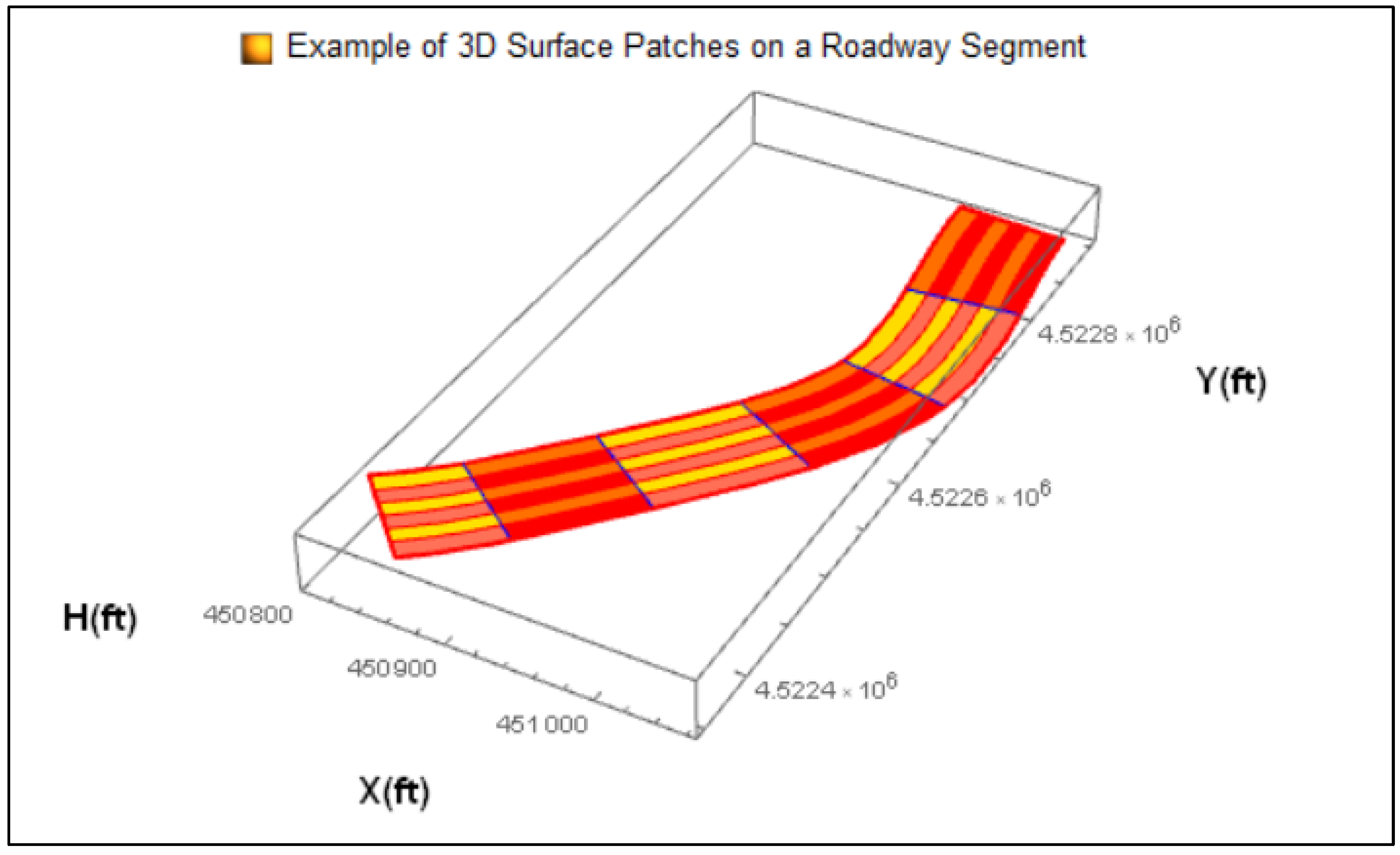
After the 3-D B-spline is defined, it must be divided into sub-surfaces which, in line with differential geometry terminology, are called surface “patches”. Patches are simply curvilinear polygons on a 3-D surface, but in this case these curvilinear polygons are more explicitly and specifically defined as curvilinear rectangles because the u- and v-parametric curves will be defined in such a way that they will be perpendicular to each other. The division of the road surface into patches has a basic advantage in terms of creating unique small areas of the roadway surface where each crash could be allocated and thus allow for the correlation of the parameters in the model estimation. In addition, the areas where zero crashes have occurred will also be analyzed, i.e., the crash frequency will not be inflated. The latter rationale is in fact the basic logic that spatial statistics are based upon. As a final note, the number of patches will directly define the sample size of the dataset through a one-to-one relationship. An example of surface patches is presented in Figure 3.1.

The 3-D geometric metrics for each patch will be calculated as the arithmetic average of the respective 3-D metrics of nine points: the four vertices which define each particular patch, the four median points between the four patch vertices, and the point in the center of the patch. For example, the Gaussian curvature of a patch will be calculated as the average Gaussian curvatures corresponding to these points. However, for each crash in addition to considering the Gaussian curvature, or any other 3-D metric that will be examined, of the specific patch where the crash occurred, the values of the surrounding patches will also be considered.

When a crash occurs, it can be reasonably argued that not only does the specific geographic point where the crash occurred matter, but the preceding and following geometry of the roadway could also have an effect. It would be therefore somewhat simplistic not to consider the geometric characteristics of the roadway before and after the crash occurrence location. For this reason, the 3-D metrics of the surrounding patches will also be considered as contributing in the final calculation of the 3-D metrics of the each patch with associated weights. The patch where the crash occurred will be called the “principal patch”. A question that arises is how the 3-D metrics will be finally calculated. The weight allocation for the final averaged 3-D metrics will be made as follows: the principal patch will have a weight of 2, whereas the patches exactly before and after the “principal patch” will have a weight of 1. Therefore, the 3-D geometric metrics corresponding to each patch will be calculated based on a weighted average of the principal and surrounding, i.e., preceding and following, patches.

Figure 2.1. Example of 3-D Surface Patches on a Roadway Segment.

Figure 2.1. Example of 3-D Surface Patches on a Roadway Segment.

At this point, all patches have a value for each 3-D metric that will be examined in the statistical analysis, i.e. Gaussian curvature, mean curvature, 3-D curvature, torsion, geodesic curvature, normal curvature, etc. The next step will allocate the crashes to their corresponding patches. Initially, the coordinates of the crashes, which are downloaded from the Kentucky State Police website in the form of geographic coordinates, are converted to Cartesian coordinates. The problem of checking whether a point lies inside a polygon is a classical problem in the field of computational geometry and is called the Point-In-Polygon (PIP) problem. The solution to this is achieved with the use of the Jordan Curve Theorem. The algorithm has been developed and applied in Mathematica in previous research (Amiridis and Psarianos 2016) and it is readily available. By applying the PIP algorithm, all crashes will be linked to their respective patch and after the crashes have been allocated accordingly, the sum of crashes for each patch will be calculated. The sum of crashes for each patch will finally be the response variable in the statistical model development.

2.7. Model Development

The model development lies in the core of this research since its objective is to suggest robust statistical models that can predict the number of crashes in a given roadway segment with specific geometric characteristics using 3-D model metrics. The response variable will be the total number of crashes in each patch. The patch length will affect the sample size for the analysis and a thorough analysis will be undertaken to determine the optimum length for prediction. A count regression model will be developed since the response variable, i.e. crashes, is such. As noted in the previous chapter, the most common count models used in road safety research are the Poisson and Negative Binomial regression models. In crash data there is, almost always, an issue of over-dispersion: the variance is statistically larger than the mean. The issue of over-dispersion often appears when there is a large number of zeros in the dataset, a case that is prevalent when dealing with crash data. The Negative Binomial distribution can account the over-dispersion in a dataset since it has an additional parameter, i.e., dispersion parameter, which is used to model the variance. The Negative Binomial regression can be viewed as an alternative strategy of modeling over-dispersed data that follow a Poisson distribution. The latter observation means that a very important underlying assumption regarding the errors, produced from the Negative Binomial regression, is that they must follow the Poisson distribution. Alternatively, the conditional distribution of the response variable must follow the Poisson distribution, but this assumption is practically impossible to be tested since the probability distributions of the explanatory variables are unknown. In this case, the error/residual approach is the most pertinent method, since the effect of the explanatory variables is “filtered out”, in order to assess one of the most essential underlying assumptions of the Negative Binomial Regression model. Although there are a number of other approaches to deal with over-dispersed data, such as the quasi Poisson and Gamma regression models, the Negative Binomial regression will most likely be the final type of regression to be used since it is the most commonly used and accepted model for crash data analysis in the road safety research community as previously noted. In fact, the assessment of the underlying assumptions of the Negative Binomial Regression model, which is an essential task in any statistical analysis, has been extensively studied in prior research aiming to predict the number of crashes at signalized intersections with permitted, protected, and permitted/protected left-turn phasing schemes (Amiridis 2016; Amiridis et al. 2017).

There are several 3-D metrics that could be tested as explanatory variables such as:

• Gaussian curvature
• Mean curvature
• Length of geodesic curves
• Metrics of the First Fundamental Form
• Metrics of the Second Fundamental Form
• 3-D curvature
• Torsion
• Geodesic curvature
• Normal curvature
• Pseudo-geodesic curvature
• Pseudo-normal curvature
• Darboux vector metric, i.e., vector of angular velocity

These variables are well known metrics and thoroughly described in any typical differential geometry textbook. However, the interesting aspect here is to emphasize their equivalence to roadway geometric elements such as the radius, grade, superelevation etc. Two examples of the analogy/equivalence between 2-D and 3-D metrics have already been discussed above regarding the 2-D analogy of pseudo-geodesic and pseudo-normal curvature (Amiridis and Psarianos 2015a). In addition, some of these 3-D metrics have the potential to allow for incorporating more than one geometric traditional element and this will be explored and presented in this research. For example, the Gaussian curvature can capture the three-way interaction of the horizontal, vertical alignment, and the superelevation in one single value.

One of the goals of this research is to develop models that are surface-based, i.e., not only curve -based. The analysis here is not intended to simply analyze 3-D metrics, but rather to analyze 3-D surface oriented metrics, which can be calculated only on a 3-D surface, and then be used as crash predictors. In this way, all geometric combinations that may be produced by the interaction among the horizontal alignment, vertical alignment, and cross slopes including superelevation rate, will be implicitly expressed by single variables. Considering this concept, the potential 3-D surface variables that could be analyzed are the following:

• Gaussian curvature
• Mean curvature
• Metrics of the First Fundamental Form
• Metrics of the Second Fundamental Form
• Geodesic curvature
• Normal curvature

It is noted that the geodesic and normal curvatures can resemble, in a not strictly accurate but adequate enough manner, the horizontal and vertical curvatures, respectively. However, the intent with this research is to move away from anything that may be linked to the 2-D conventional approach and investigate metrics in which more rich geometric information is hidden. Therefore, the last two variables will not be considered, since they are essentially 2-D variables that are calculated planes that are tangent on 3-D surfaces. In addition, the Gaussian and Mean Curvatures are explicitly defined by the metrics of the First and Second Fundamental Forms where the effect of the metrics of the First and Second Fundamental Forms is “nested” into the Gaussian and Mean Curvature (Lipschutz 1981). Therefore, the potential explanatory variables that will be used are the Gaussian Curvature and the Mean Curvature. An overview, i.e., definition and properties, of the Gaussian and Mean curvature is briefly presented, without the inclusion of strict mathematical proofs, in Appendix A.

The entire analysis is “patch-based” and therefore a crucial task is the determination of the most pertinent patch length. In order to address this question, six patch lengths will be tested: 1,500 ft, 1,000 ft, 400ft, 200ft, 100 ft, and 50 ft. Because of length restrictions, it is noted beforehand that the 100 ft. patch length turned out to be the most pertinent. The attempts to define the optimal length and associated statistical analysis to identify this are described in detail in Amiridis, K. (2019). The rule used to address is that the closer the predicted crashes are to the actual/observed crashes, the higher the predictive power of the model. The comparison between predicted and observed crashes is achieved by developing models using 13 years of the crash data and then comparing their prediction to the crashes of the 14^th remainder year. However, the final proposed model and the final explanatory variables that will enter the model will be based on all 14 years. As a final note, the scale of the covariates, i.e., whether the explanatory variable should be raised to a power or an exponential transformation would be more pertinent, was determined according to their respective “grouped” frequency tables. The rational of this approach is discussed in the next chapter in more detail.

2.8. Comparison to Current Safety Estimations

The final task of the dissertation is to compare the suggested prediction models with the crash prediction results that would be produced from the existing models presented in the HSM (AASHTO 2010). In fact, the results will be compared to the predicted crashes from the IHSDM software, which can also utilize the historical crashes that are available from 2004-2017. The comparison will be conducted with training data: for each roadway, one year at a time will be kept outside of the analysis and then the crashes for that year, whose actual/observed crashes are known, will be predicted based on the data of the remaining years. For example, for a given roadway segment, in order to evaluate the predictive accuracy for 2017, the crashes of this year will be removed from the model development that will utilize only the crashes in the 2004-2016 period. Since there are seven roadway segments and 14 years of available crash data, 98 prediction evaluations will be essentially developed. Finally, this procedure allows for comparing the predictive power and accuracy of the proposed modelling approach with the current practices as described in the HSM.

3. Crash Prediction Model

This chapter presents the development of the models for crash predictions utilizing the 3-D B-spline roadway surface. To achieve this, three roadway segments are utilized. The following sections present the data used and the analysis undertaken to develop the 3-D SPF models.

3.1. Model Data

3.1.1. Geometric Data

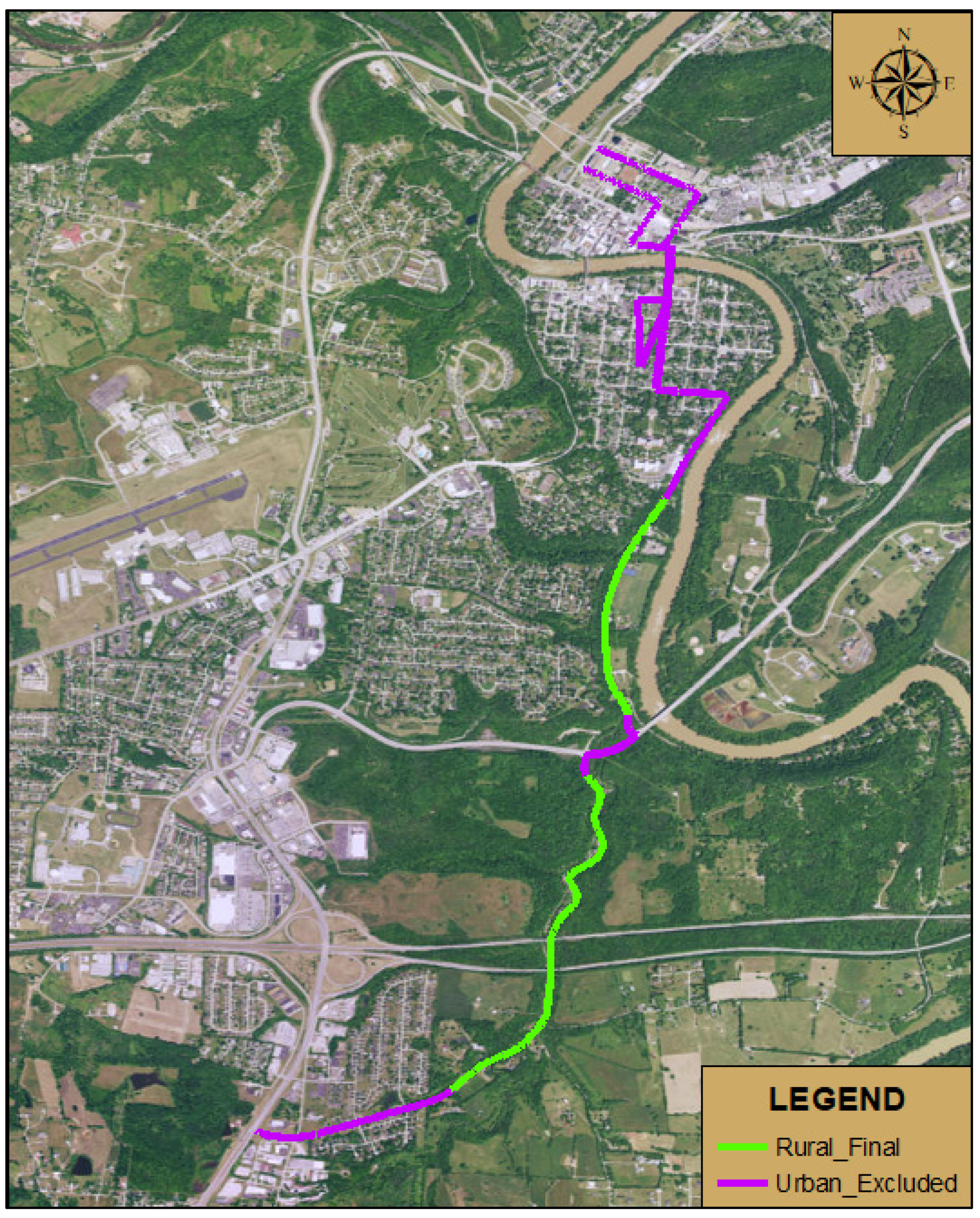
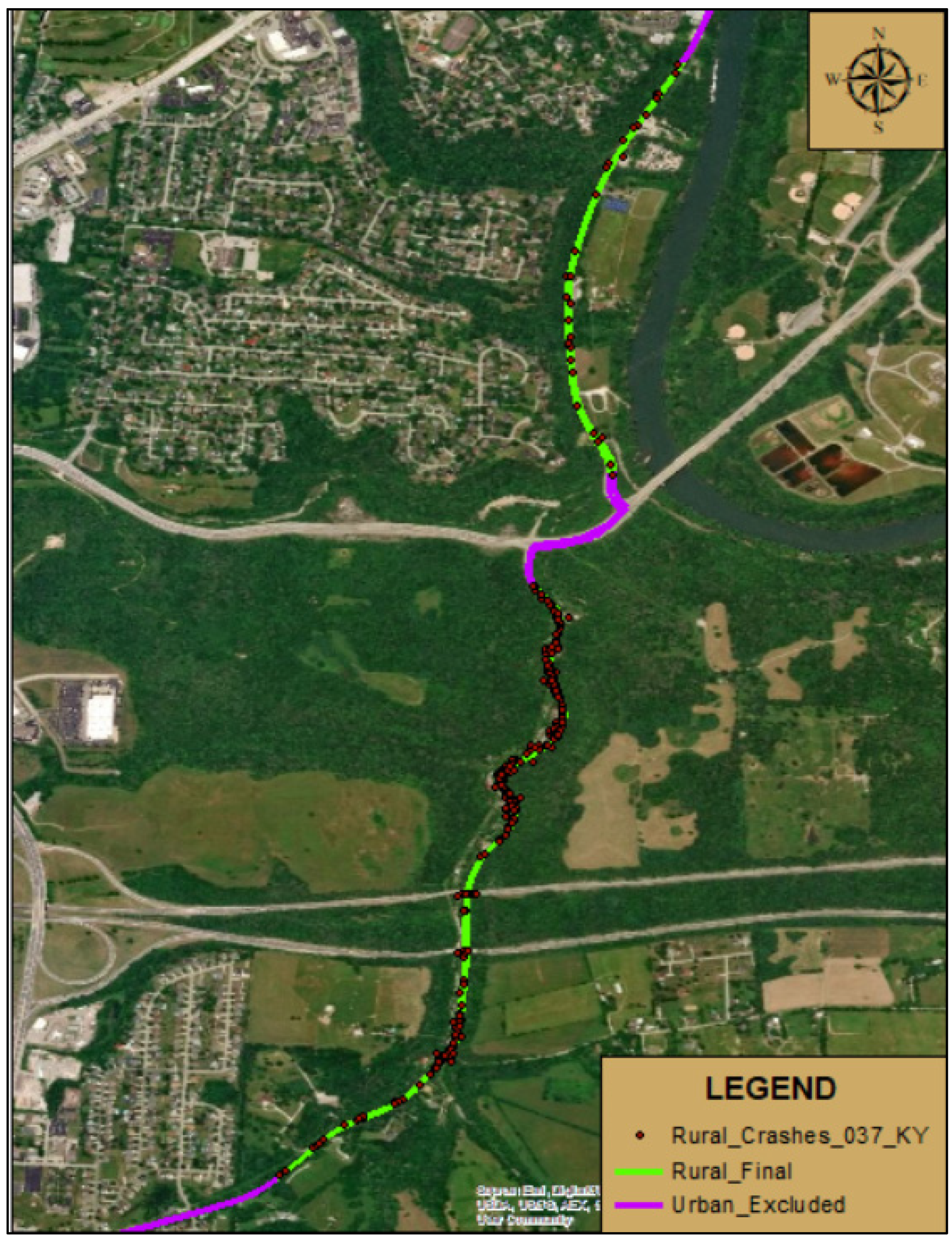
The ArcGIS platform will be used to display the three roadway segments used in order to determine the rural sections for the analysis. The urban (built-up) sections of the roadways selected were visually identified and excluded from the analysis. Specifically, an additional length of 400 ft was excluded from the beginning and end of each urban section in order to filter out the potential “urban effect”. Finally, a 400 ft radius was used to exclude major intersections to obtain only continuous roadway segments. Google Earth .kmz files were used to depict the roadway segments (they are detailed in Amiridis, K. 2019, Appendix B.

An example of the process undertaken to develop the sections for study is shown here. Figure 4.1, shows the data for KY 420 indicating the rural and urban sections of the roadway. The urban and rural sections of all roadway segments under study are shown in Appendix C. Each of the roadway segments considered was evaluated to determine whether there have been any geometric alterations during the study period. The review identified that there were no changes in the alignments over the 2004-2017 period. This allows for an accurate comparison throughout the entire period of the study. If geometric changes were present, then separate 3-D roadway models would have to be developed in order to capture these changes.

Figure 4. 1. Example of Rural/Urban Distinction (KY 420).

Figure 4. 1. Example of Rural/Urban Distinction (KY 420).

The next step involved the development of the 3-D B-spline centerline of the first section (Figure 4.2) and the corresponding 3-D B-spline surface of the roadway segment (Figure 4.3) while considering the superelevation rate of the curves. This process resulted in seven separate roadway segments that were geometrically modeled and statistically analyzed. The 3-D representations of the roadway centerlines and surfaces, as modeled in the Mathematica platform, for all seven segments (detailed in Amiridis, K. 2019, Appendix C). The travel lane width is assumed to be 11 ft according to multiple measurements along the roadway segments, whereas the centerline lengths of these sections are shown in Table 4.1.

Figure 4. 2. 3-D B-Spline Roadway Centerline (KY420-1).

Figure 4. 2. 3-D B-Spline Roadway Centerline (KY420-1).

Figure 4. 3. 3-D B-Spline Roadway Surface (KY420-1).

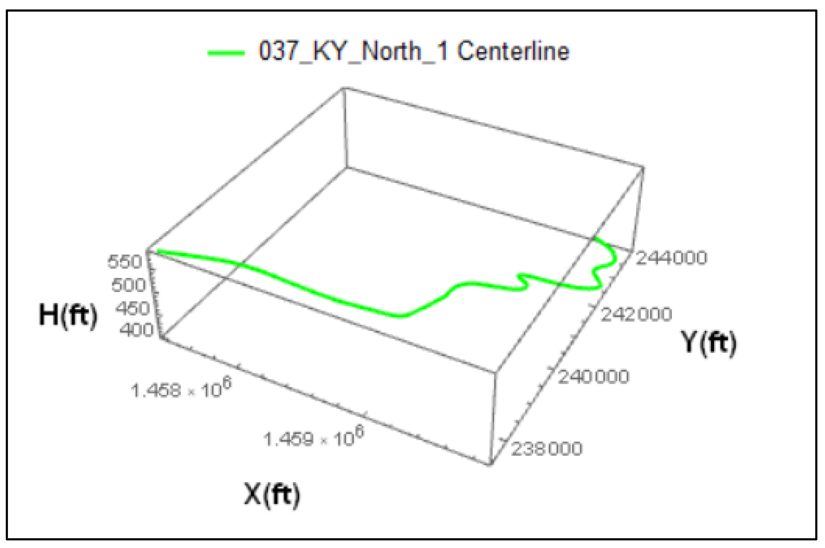
Figure 4. 3. 3-D B-Spline Roadway Surface (KY420-1).

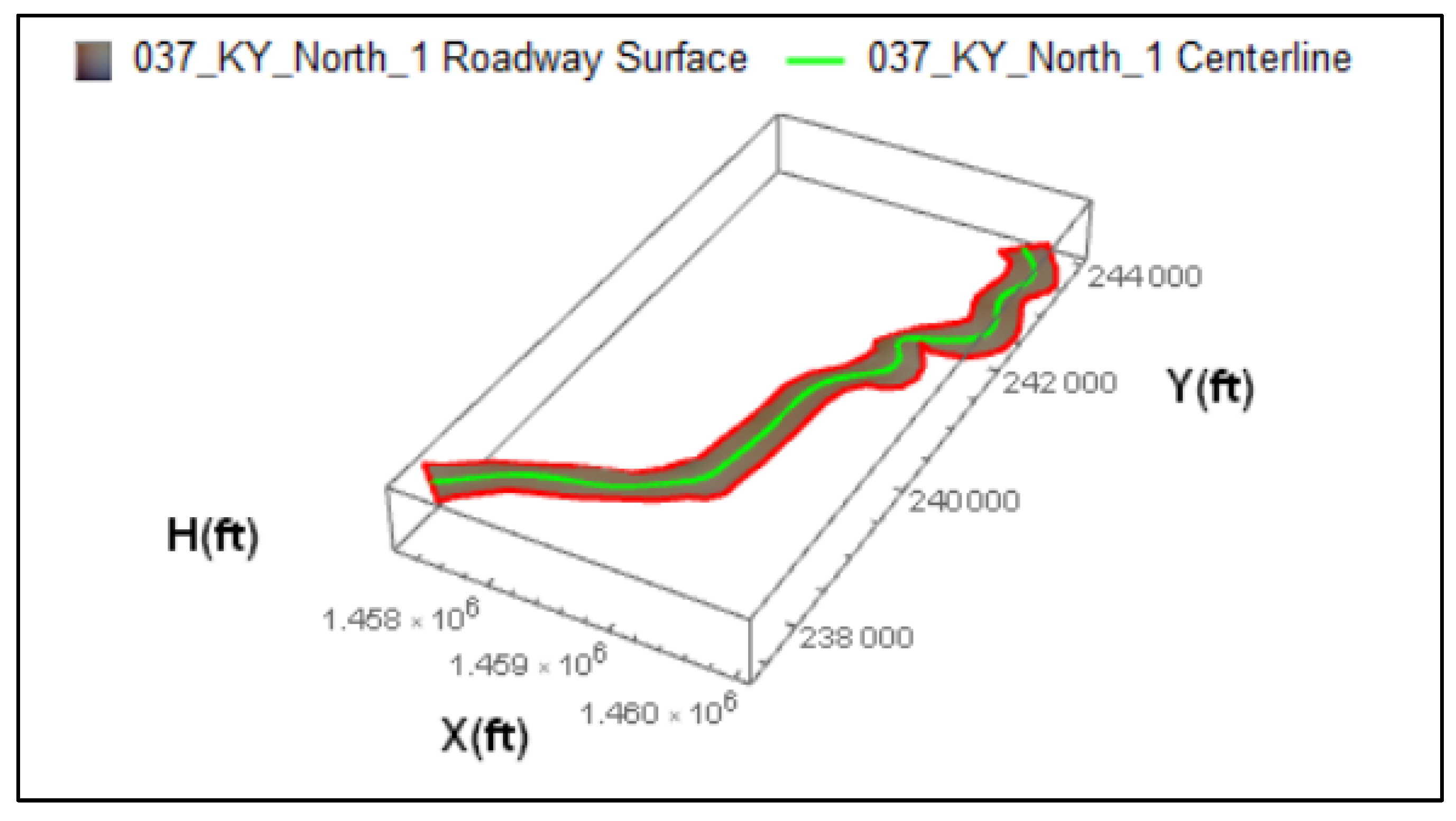
Table 4. 1. Roadway Segment Lengths.

Roadway	Roadway Segment	Length (miles)
KY 420	KY420-1	1.4119
	KY420-2	0.8783
KY 152	KY152-1	8.6922
	KY152-2	2.2392
	KY152-3	3.3862
US 68	US68-1	5.7450
	US68-2	11.5097
Total		33.8625

Table 4. 1. Roadway Segment Lengths.

Roadway	Roadway Segment	Length (miles)
KY 420	KY420-1	1.4119
	KY420-2	0.8783
KY 152	KY152-1	8.6922
	KY152-2	2.2392
	KY152-3	3.3862
US 68	US68-1	5.7450
	US68-2	11.5097
Total		33.8625

3.1.2. Crash Data

The crash data for each section for the 2004 to 2017 period were retrieved from the Kentucky State Police Wizard. The crashes were plotted with ArcGIS and an example is shown in Figure 4.4.

Figure 4. 4. Example of Crash Data Plots (KY 420).

Figure 4. 4. Example of Crash Data Plots (KY 420).

The crash plots for all the other segments are detailed in Amiridis, K. 2019, Appendix D. Table 4.2 presents a summary of the crash data by type and other characteristics.

Table 4. 2. Crash Summary (Percentages).

	Roadway Segment
	KY420-1	KY420-2	KY152-1	KY152-2	KY152-3	US68-1	US68-2
	Crash Type
Single Vehicle	73	60	76	61	77	80	75
Rear End	10	8	5	18	2	3	4
Angle	6	16	4	5	2	6	5
Sideswipe Opp. Dir.	6	3	10	12	11	6	8
Head On	4	0	1	0	4	2	4
Sideswipe Same Dir.	1	11	3	4	2	2	2
Other	0	2	1	0	2	1	2
	Number of Motor Vehicles
Single	73	60	76	56	77	80	74
Two	26	35	23	39	22	20	24
Multi	1	5	1	5	1	0	2
	Crash Severity
PDO	77.0	83.8	74.5	68.2	67.0	74.7	75.7
Injury	22.7	13.5	22.2	31.8	30.9	24.2	24.0
Fatal	0.3	2.7	3.3	0.0	2.1	1.1	0.3
	Roadway Alignment
Curve & Grade	46	11	32	23	31	50	45
Curve & Hill Crest	6	0	4	14	6	5	5
Curve & Level	35	14	20	5	33	26	20
Straight & Grade	10	5	20	25	14	8	10
Straight & Hill Crest	1	0	6	25	3	0	3
Straight & Level	2	70	19	8	13	11	17

Table 4. 2. Crash Summary (Percentages).

	Roadway Segment
	KY420-1	KY420-2	KY152-1	KY152-2	KY152-3	US68-1	US68-2
	Crash Type
Single Vehicle	73	60	76	61	77	80	75
Rear End	10	8	5	18	2	3	4
Angle	6	16	4	5	2	6	5
Sideswipe Opp. Dir.	6	3	10	12	11	6	8
Head On	4	0	1	0	4	2	4
Sideswipe Same Dir.	1	11	3	4	2	2	2
Other	0	2	1	0	2	1	2
	Number of Motor Vehicles
Single	73	60	76	56	77	80	74
Two	26	35	23	39	22	20	24
Multi	1	5	1	5	1	0	2
	Crash Severity
PDO	77.0	83.8	74.5	68.2	67.0	74.7	75.7
Injury	22.7	13.5	22.2	31.8	30.9	24.2	24.0
Fatal	0.3	2.7	3.3	0.0	2.1	1.1	0.3
	Roadway Alignment
Curve & Grade	46	11	32	23	31	50	45
Curve & Hill Crest	6	0	4	14	6	5	5
Curve & Level	35	14	20	5	33	26	20
Straight & Grade	10	5	20	25	14	8	10
Straight & Hill Crest	1	0	6	25	3	0	3
Straight & Level	2	70	19	8	13	11	17

The data in Table 4.2 indicate that the majority of crashes are “Single Vehicle”. This fact is advantageous for the intended analysis and overall research because this specific crash type is mostly related to the geometric characteristics of a roadway. Table 4.2 also shows that approximately 85 percent of the crashes were related to some combination of the horizontal and vertical alignment. This verifies once again the need, as emphasized also in previous research, of investigating the effects of horizontal and vertical coordination in a more systematic manner to address safety concerns. This further supports the need for considering 3-D solutions and the value of this research proposal. Finally, in terms of severity level, it is worth mentioning that from the total crashes that occurred, 75 percent are property damage only, 24 percent resulted in some kind of injury, whereas only a small percentage (1 percent) resulted in fatalities.

3.1.3. AADT Data Needs

The AADT for each section was obtained from the KYTC. Initially, the corresponding AADT stations for each roadway had to be identified through the interactive map provided by KYTC and the starting longitude and latitude coordinates in order to retrieve the corresponding AADT values. The AADT values were linked to each segment separately; an example of the AADT data is shown in Table 4.3 for a specific station for KY 420. It should be noted that the AADT was not available for all years, i.e. 2004-2017 and that the missing data were estimated by applying piecewise polynomial cubic spline interpolations between known values. Similar AADT data were retrieved from all associated stations and for all roadway segments (detailed in Amiridis 2019, Appendix E).

Table 4. 3. AADT Data for Station ID# 037553; KY 420-1.

Year	AADT
2004	5051
2005	5220
2006	5262
2007	5214
2008	5110
2009	4988
2010	4882
2011	4830
2012	4962
2013	5147
2014	5351
2015	5537
2016	5671
2017	5716

Note: Bold numbers are actual AADT counts.

Table 4. 3. AADT Data for Station ID# 037553; KY 420-1.

Year	AADT
2004	5051
2005	5220
2006	5262
2007	5214
2008	5110
2009	4988
2010	4882
2011	4830
2012	4962
2013	5147
2014	5351
2015	5537
2016	5671
2017	5716

Note: Bold numbers are actual AADT counts.

3.2. Statistical Analysis

This section describes the way in which the final crash prediction models are developed. As noted above, six patch lengths, i.e. 1,500 ft, 1,000 ft, 400 ft, 200 ft, 100 ft, and 50 ft were considered. The length of the patch length denoted the way in which the 3-D roadway surface is spatially divided. However, no matter the patch length, in each patch there are four explanatory variables linked to it, namely: Number of crashes that occurred, AADT value, Gaussian Curvature (GC), and Mean Curvature (MC). In addition to the initial values of these variables, transformations were also considered, e.g. AADT², GC² MC³ in order to identify the optimal scale and combination of these variables. All of these transformations and the justification of the optimal scale are presented in Amiridis, K. 2019, Appendix F. Moreover, statistical interactions of the explanatory variables, e.g. Gaussian*Mean, are also considered. Finally, it should be noted here that the statistical regression model that was utilized is the Negative Binomial Regression because over-dispersion is present in the data and because it was intended to keep the statistics rather simple in order to retain the focus of the research on the use of 3-D geometric explanatory variables in highway safety rather than the statistical methods utilized per se. After all, the typical regression model that is utilized for crash prediction modeling is indeed the Negative Binomial Regression.

The analysis conducted will serve a dual purpose: 1) demonstrate the proof-of-concept of the proposed 3-D approach; and 2) evaluate the predictive power of the model. These two objectives can be viewed as independent, i.e., failure in demonstrating predictive power of the model does not mean that the proof-of-concept is violated. For example, 3-D metrics may be proven to have a statistically significant effect in crash modeling, but the reason for potential failure in adequately predicting actual crashes may simply rest on the fact that more explanatory variables are required in the model. The proof-of-concept relies on the verification that the 3-D differential geometry metrics of Gaussian and Mean curvature are statistically significant crash predictors. This can be successfully demonstrated if it is proven that the coefficients of the metrics are indeed statistically significant. It should be also noted that depending on whether historical crashes are available, two strategies come into play in order to predict crashes in the most effective way.

3.2.1. Proof-of-Concept

In order to provide the proof-of-concept in the most concrete way, all years, i.e. 2004-2017, and all seven roadways entered the same model which will be called “Integrated Model” (IM) to be distinguished from the models that will be developed for the second objective, i.e., prediction evaluation. The objective of this effort was to establish that it is meaningful to incorporate 3-D highway geometry in crash prediction models. Although the predictive power of the model was not evaluated at this point, this step was crucial because failure to address the statistical significance of the 3-D metrics in crash prediction, would yield any further discussion of prediction power evaluation meaningless. Moreover, the type of the final explanatory variables that will enter this model will function as the basis of the predictive power evaluation of the model. For example, if the variables, AADT, Gaussian², and Mean³ are proven to be the finalists, then these exact variables would be considered in order to evaluate the predictive power of the model; a logic that holds true in most predictive models. For example, even for the variables than come into play in the SPFs in the HSM with a specific transformation, e.g., exp(AADT), does not mean that this particular transformation is the optimal in all cases; it simply means that this transformation is on average adequate.

Although not explicitly stated, a part of the statistical analysis essentially touches the field of spatial statistics since the selection of an acceptable patch length is of utmost importance because it functions as the basis of all further (traditional) statistical analysis. To proceed with this effort, a two-stage simultaneous testing was undertaken that would define the optimal patch length and model to be used. First, for each patch length considered, models with the variables of interest were developed and the most appropriate was selected in terms of statistical significance and the Akaike Information Criterion (AIC) evaluation criterion. Second, these models were then compared to identify the most appropriate patch for analysis and power of prediction evaluation. Since there are six patch lengths tested, six “final models” will eventually be compared to each other.

All of the combinations of the explanatory variables that were utilized until the final model was decided, for all patch length combinations, are detailed in Amiridis, K. 2019, Appendix G. The criterion according to which the models were compared was the AIC; the lower the AIC, the more informationally rich the model is. The AIC also functions as an adjusted R-square in the sense that it penalizes the number of variables that enter the model. Furthermore, in order for a model to be further considered as a finalist for additional evaluation, all of the coefficients of the explanatory variables that enter the model must be statistically significant, i.e., p-value<0.05. The demand of p-value<0.05 is associated with the fact that a significance level of 5% is considered; in fact, each p-value, depending on the number of explanatory variables that enter the model, must be less than the predefined “familywise” p-value, which in this case is set to 0.05, according to the Bonferroni, or any other type, correction (Myers et al. 2010). Roughly speaking, this means that if two explanatory variables are considered then the p-value of the coefficient of each variable must be less than approximately 0.025 $(=1-\sqrt{0.95}$) assuming that the two explanatory variables are independent in order for the “overall p-value” to be less than 0.05.

More generally, the Bonferroni correction, or any other type of correction, should be applied when explanatory variables are simultaneously inserted in a statistical model. More specifically, the significance level has been assumed to be 5 percent, i.e., there is a 95 percent confidence that the true parameters belong in the constructed confidence interval. However, the significance level of 5% should not be applied to each coefficient, but to the model as a whole; therefore, in order for the significance level of the whole model to be kept at the 5 percent significance level, the p-value of each coefficient should be less than 5 percent. The value of each p-value in order to achieve a “family-wise” error of 5 percent is imposed by the pertinent correction method used, e.g. Bonferroni, Tukey, and by the number of variables; the more variables, the stricter, i.e. less, the p-value must be.

It should be noted here that the AADT, GC and MC are to be used as explanatory variables, i.e. main effects, in the statistical analysis through a multivariate regression analysis. However, even when multiple explanatory variables are intended to enter the model, the analysis should always begin by visualizing the explanatory variables vs. the dependent variable. The Negative Binomial Regression, which is the regression type that will be applied here is a member of the family of Generalized Linear Models (GLMs). Each regression member of the GLMs is associated with a function that is called the “canonical link function”, which actually represents the optimal transformation that should be applied to the dependent variable in order to satisfy desirable statistical properties such as unbiased parameters (Hardin and Hilbe 2012). In the case of the Poisson and Negative Binomial Regression, the aforementioned function is indeed the “log-link function”. If the logarithmic transformation is not applied to the dependent variable, then the so-called “identity link function” is applied, meaning that the dependent variable is simply the variable “Crashes”. Results will be produced even if the log-link function is not applied but the reliability of the results is weakened because the log-link function is the “canonical” link function for the Negative Binomial Regression. This is why the Poisson and Negative Binomial regression models are also often called log-linear models, meaning that the explanatory variables have a linear relationship with the logarithm of the dependent variable. Therefore, in this case the dependent variable will be LN(crashes).

The typical visualization process in order to identify the optimal transformation of each explanatory variables is via scatterplots. The scatterplots for the explanatory variables AADT, GC, and MC are shown in Figure 4.7, Figure 4.8 and Figure 4.9 respectively for the 100 ft patch.

Figure 4. 5. Scatterplot LN(Crashes) vs. AADT_Binned.

Figure 4. 5. Scatterplot LN(Crashes) vs. AADT_Binned.

Figure 4. 6. Scatterplot LN(Crashes) vs. Average GC- Binned.

Figure 4. 6. Scatterplot LN(Crashes) vs. Average GC- Binned.

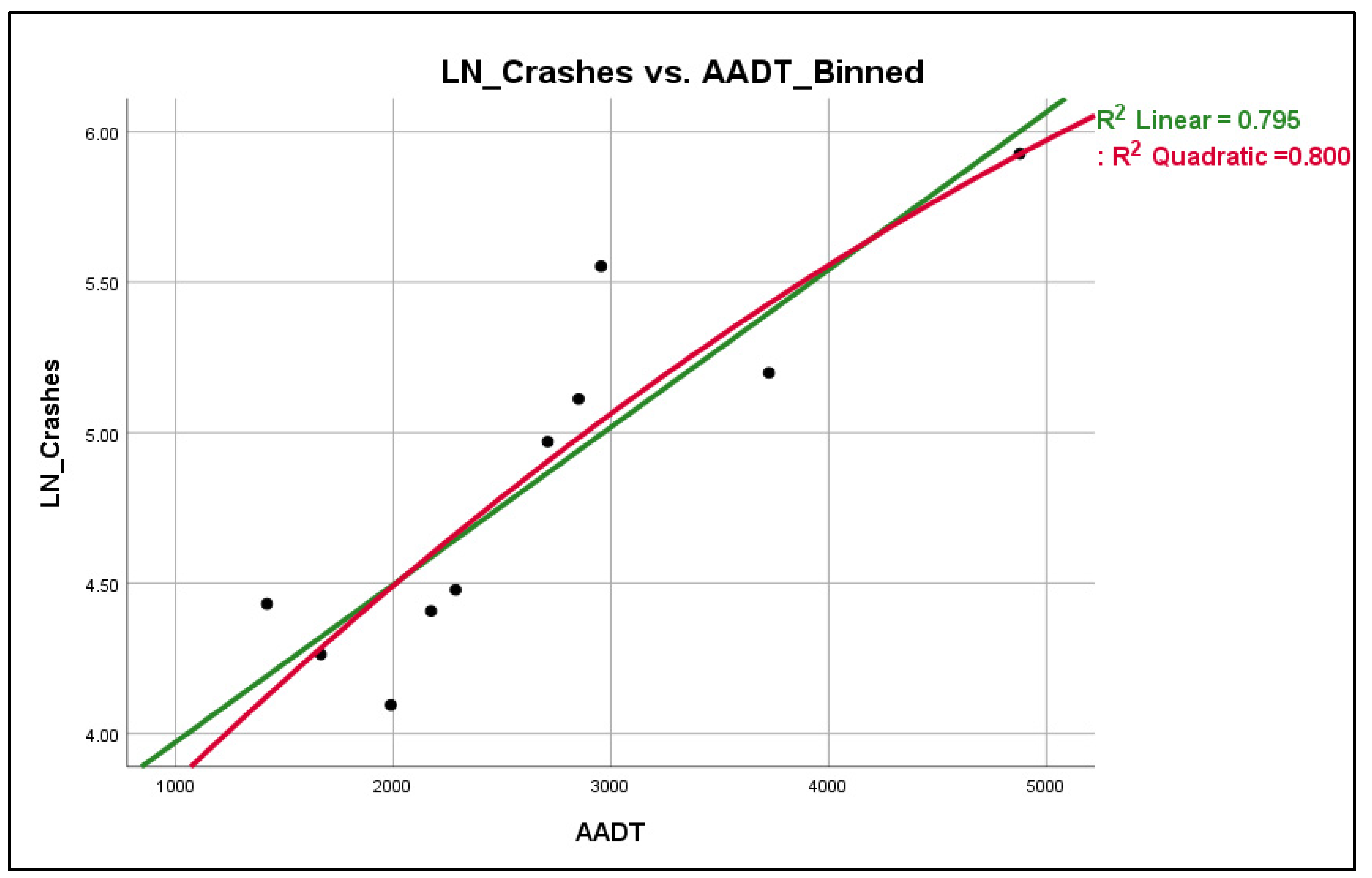
Figure 4. 7. Scatterplot LN(Crashes) vs. Average MC _Binned.

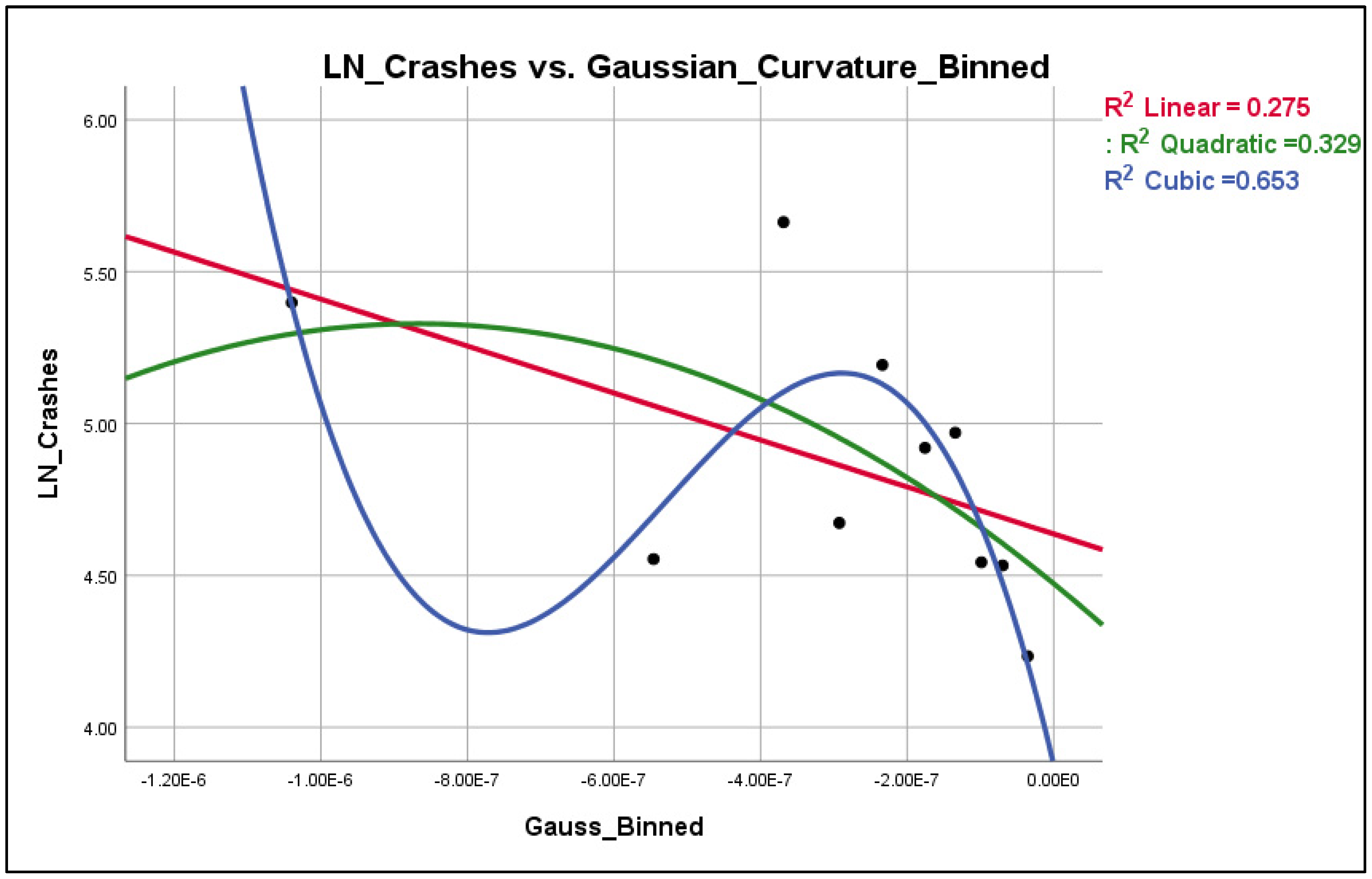
Figure 4. 7. Scatterplot LN(Crashes) vs. Average MC _Binned.

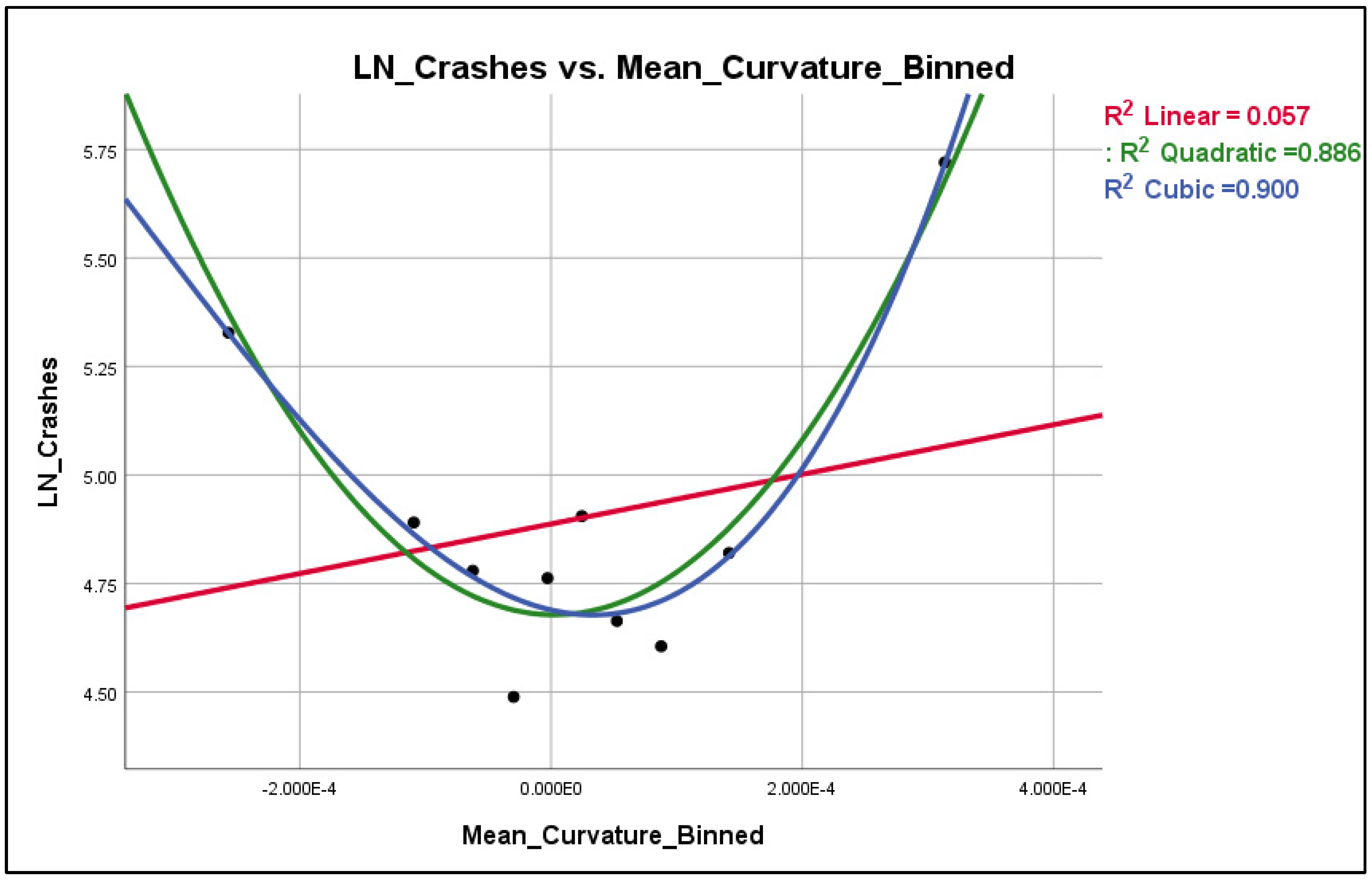
According to Figure 4.7, the AADT seems to have a rather linear relationship with LN(crashes), whereas the Gaussian curvature (Figure 4.8) seems to have a cubic relationship with LN(crashes) and the Mean curvature (Figure 4.9) has an essentially quadratic relationship with LN(crashes). However, these observations hold true only when the explanatory variables are plotted one by one against the dependent variable; in other words, there is no guarantee that the nature of these relationships will remain the same when all the explanatory variables enter the model. However, this procedure has revealed that, especially for the Mean and Gaussian curvature, there is some indication that their relationship may not be linear in nature with LN(crashes) and therefore quadratic and cubic transformations may be appropriate for testing.

For each patch, 38 variable combinations were tested until the analysis was finalized. The models considered each variable alone and in a variety of combinations in order to determine the most appropriate and meaningful combination. All these combinations for each patch length are presented in Amiridis, K. 2019, Appendix G. The process for determining whether a model was appropriate was based on an initial determination of whether all the coefficients of the model were statistically significant and accounting for the Bonferroni correction. Then the statistically significant models were compared with the AIC criterion. It is noted that, as a rule of thumb, when two models are compared and their AICs difference is greater than 10, then this difference is “significant”, meaning that the model with the lowest AIC should be kept instead (Hardin and Hilbe 2012). Finally, the assumptions according to which the model is based, e.g., normality of deviance residual distribution, must also be satisfied.

A summary of the variables used in the best models for each patch length are summarized in Table 4.5. The final suggested models as shown in Table 4.5 indicate that the Gaussian Curvature (GC) and Mean Curvature (MC) of 3-D surfaces play a crucial role in crash prediction since they are statistically significant in all models, in which the Bonferroni correction has also been accounted for. In fact, not only are the Gaussian and Mean Curvature statistically significant in all models, but their p-values are also less than 0.001 in all models. The insertion of these two differential geometry metrics it is actually the new aspect that this research introduces to the literature. The use of these metrics can be considered promising because the Gaussian and Mean curvatures are the cornerstones of the study of 3-D mathematical surfaces as a whole in differential geometry. Moreover, the fact that transformed geometric metric, e.g. GC³ and MC², and that the 2-way interaction term GC*MC insert the model, in the 100 ft patch length model, emphasizes the complexity by which roadway geometry affects crash occurrence, a fact that cannot be revealed in such an explicit manner through conventional 2-D geometric metrics. Finally, in terms of computational statistics stability, when a variable is entered in a model with a power, e.g., quadratic, it is beneficial if the “lower power terms” are also included in the model, e.g. linear, for computational reasons. Fortunately, this is the case for both the GC³ and MC² variables since the variables GC² and GC, as well as MC are also included in the model with p-values<0.001, meaning that even the Bonferroni correction is amply satisfied.

Table 4. 4. Variables Present in Final Best Models for Each Patch Length.

Patch length	Explanatory Variables
	AADT	GC	MC	GC2	GC3	MC2	MC3	AADT*MC	GC*MC
1500	X	X	X	X	X
1000	X	X		X	X		X
400	X	X	X	X	X	X
200	X	X	X	X	X			X
100	X	X	X	X	X	X			X
50	X	X	X	X	X	X			X

Table 4. 4. Variables Present in Final Best Models for Each Patch Length.

Patch length	Explanatory Variables
	AADT	GC	MC	GC2	GC3	MC2	MC3	AADT*MC	GC*MC
1500	X	X	X	X	X
1000	X	X		X	X		X
400	X	X	X	X	X	X
200	X	X	X	X	X			X
100	X	X	X	X	X	X			X
50	X	X	X	X	X	X			X

The criterion used in order to select the most appropriate patch length was based on the overall error prediction which is estimated as the difference between the observed and model-predicted number of crashes. A summary of the predictive ability of each patch length, i.e., the associated error percentage to each, is shown in Table 4.6; it is noted that 1,534 crashes occurred during the 2004-2017 period. Although it may be considered adequate on a practical basis to conclude that the 100 ft patch is the most pertinent patch length for the analysis, an additional statistical metric will also be considered to further validate this assertion, for the comparison among the different patch lengths. The additional statistical measurement used is the Predicted Error Sum of Squares or the so-called PRESS (Caroni and Oikonomou 2017). PRESS is used in order to compare regression models in terms of their ability to predict new values; the model preferred is the one with the smallest value of PRESS (Table 4.6).

Table 4. 5. Patch Length Comparison in Terms of Predictive Ability.

Patch Length (ft)	Predicted Crashes	Error Percentage of Total Crashes Predicted	PRESS
1,500	1,295	-15.6%	81.94
1,000	1,342	-12.5%	51.63
400	1,582	3.1%	47.40
200	1,546	0.8%	20.90
100	1,532	-0.1%	15.93
50	1,532	-0.1%	15.76

Table 4. 5. Patch Length Comparison in Terms of Predictive Ability.

Patch Length (ft)	Predicted Crashes	Error Percentage of Total Crashes Predicted	PRESS
1,500	1,295	-15.6%	81.94
1,000	1,342	-12.5%	51.63
400	1,582	3.1%	47.40
200	1,546	0.8%	20.90
100	1,532	-0.1%	15.93
50	1,532	-0.1%	15.76

The selected patch length for the final model corresponds to a length of 100 ft because it was observed that this patch length provides the best modeling ability. Even though a smaller patch length leads to an increase in the predictive power of the model, this was true up to a “cut-off” patch length, which in this case was estimated to be 50 ft. In this case, “cut-off” indicates that after a certain point the overall error is not practically improved with the reduction of the patch length.

The results of the model corresponding to the 50 ft patch were identical to the ones derived from the 100 ft patch (Table 4.6). Moreover, a 100 ft patch may be considered more appropriate for transportation related applications because vehicles that have a length over 50 ft such as combination trucks, recreational cars, and buses can be analyzed in a more reliable manner by incorporating a larger surrounding roadway geometry. Therefore, for transportation related consistency, practical effect of overall error reduction as well as computational speed purposes it was decided to utilize the 100 ft patch for the crash modeling process.

The final model corresponding to the 100 ft patch length is summarized in Table 4.7, whereas the regression model is presented in Equation 4. The AIC for the models considered ranged from 11,183 to 11,803. The final model that was kept was indeed the one with the lowest AIC of 11,183 while the second-best model had an AIC of 11,232. It is noted that all of the explanatory variables of the final have a p-value<0.001, a fact that essentially demonstrates the proof-of-concept of this research: 3-D geometric roadway metrics can successfully function as explanatory variables in crash predictive models.

Table 4. 6. Coefficient Values of Final Model (E35) for Patch Length = 100 ft.

Variable	Coefficient	p-value
(Intercept)	-4.2701	0.000
AADT	0.00037	0.000
GC	-797,670.9567	0.000
GC2	-62,371,846,845.508	0.000
GC3	-101,722,389,759,530.720	0.000
MC	347.8188	0.000
MC2	209,377.3293	0.000
GC*MC	166,612,202.0693	0.000

Table 4. 6. Coefficient Values of Final Model (E35) for Patch Length = 100 ft.

Variable	Coefficient	p-value
(Intercept)	-4.2701	0.000
AADT	0.00037	0.000
GC	-797,670.9567	0.000
GC2	-62,371,846,845.508	0.000
GC3	-101,722,389,759,530.720	0.000
MC	347.8188	0.000
MC2	209,377.3293	0.000
GC*MC	166,612,202.0693	0.000

$$LN\left(Crashes\right)=b0+b1·AADT+b2·GC+b3·{GC}^2+b4·{GC}^3+b5·MC+b6·{MC}^2+b7·\left(GC*MC\right)$$

(4)

As noted above, the presence of the Gaussian Curvature and Mean Curvature of 3-D surfaces supports the significance of these variables as crash predictors and the potential interaction with other variables; interactions that can by no means be captured in the 2-D analysis.

At this point, the “Integrated Model” in which all years and roadways are included has been finalized and presented in Equation 4 above. The IM essentially functions as a proof-of-concept for the inclusion of the 3-D metrics in crash prediction models and can, at least theoretically, be used for crash prediction purposes in other roadways. This model may be particularly useful when the purpose of an analysis is not the prediction of crashes in absolute numbers, but the comparison of alternatives, e.g. different alignments, in terms of estimating which alternative reduces crash frequency. In addition, it is suggested that the specific coefficient values (Table 4.7) be used for crash prediction purposes only when no historical crash data are available; if crash data are available for a specific roadway segment they should be certainly used in order to incorporate the “special crash pattern” in the adjusted model to be discussed in the next section. Finally, when several years of crash data are available, it is advised that, for crash prediction purposes, the years enter the model as dummy variables. The latter is suggested in order to account for seasonal and time effects. This is further discussed in the next section in which the predictive power of the model is evaluated.

3.2.2. Model Structure and Predictive Ability Evaluation

The ultimate objective of this research is the determination of the predictive ability of the proposed model based on 3-D metrics on safety predictions. The comparison is based on the crash predictions as estimated from the model and the IHSDM. The IHSDM predicts crashes per year for a given roadway through the Empirical Bayes model. To account for the differences that arise throughout the years such as the number of crashes and AADT, IHSDM needs to develop a separate prediction for each year and this approach was considered and applied in the suggested model to obtain an accurate and fair comparison. It is therefore important to consider this in the model developed here and determine how to best approach it. There are two options for incorporating the “year effect” in this analysis: 1) use a separate model for each year developing predictions one year at a time; and 2) insert dummy variables for years to account for the different AADT for each year. The following presents this analysis and the determination of which approach is more appropriate. It should be also noted that there is no concern whether the dummy variables are statistically significant or not at this point; their purpose is to simply increase the predictive ability of the model by accounting for the yearly variation of AADT and random effects in general.

The evaluation will be accomplished by creating training data, i.e., assuming that a certain year is not included in the dataset, running the analysis, and then predicting the crashes of that year and reporting the residuals. For example, the way in which the predictive power of the model will be evaluated for year 2017 is as follows. Suppose that crash data are available for years 2004-2016 and that the intention is to predict the crashes for year 2017. The predictive model will include the explanatory variables of the IM, i.e. AADT, GC, GC², GC³, MC, MC², and GC*MC. For the use of the dummy variable approach, in addition to the explanatory variables, a number of dummy variables equal to the number of years of crashes minus 1 is used. In this case, for the 13 years of available date (2004-2016 period) 12 (=13-1) dummy variables will be used. The crash predictions for year 2017 will be calculated in the following form (Equation 5):

$$LN\left(13*Crashes\right)=b0+b1·AADT+b2·GC+b3·{GC}^2+b4·{GC}^3+b5·MC+b6·{MC}^2+b7·\left(GC*MC\right)+d1·D_{2004}+\dots +d12·D_{2015}$$

(5)

or finally:

$$LN\left(Crashes\right)=b0+b1·AADT+b2·GC+b3·{GC}^2+b4·{GC}^3+b5·MC+b6·{MC}^2+b7·\left(GC*MC\right)+d1·D_{2004}+\dots +d12·D_{2015}-LN\left(13\right)$$

(6)

The term “-LN(13)” is present in Equation 6 in order to convert the prediction model on a per year basis since the model is based on 13 years of data. In statistical terminology, especially for GLM, this “-LN(13)” term is the so-called offset in the Negative Binomial Regression (Hardin and Hilbe 2012). The crash predictions for any other year will be calculated with the same exact procedure and rationale. The model structure is evaluated using both approaches, with and without dummy variables, and then comparing the predictions to the actual number of crashes. The approach that results in a prediction closer to the actual crashes would be the one to be used.

In Table 4.8 the crashes prediction breakdown per year and roadway segment is presented in which there are three columns for each roadway segment: 1) Actual Crashes (AC), 2) Predicted Crashes Without the Utilization of the Dummy Variables Approach (W/O), and 3) Predicted Crashes With the Utilization of the Dummy Variables Approach (W/). In addition, Table 4.9 presents the errors/residuals corresponding to the models with and without the dummy variable approach, as well as the corresponding Crash Improvement (CI) that has been achieved with the dummy variable approach.

Table 4. 7. Crash Predictions Estimates.

	KY420-1			KY420-2			KY152-1			KY152-2			KY152-3			US68-1			US68-2
Year	AC	W/O	W/	AC	W/O	W/	AC	W/O	W/	AC	W/O	W/	A	W/O	W/	AC	W/O	W/	AC	W/O	W/
2004	29	12	21	3	5	2	12	34	12	2	11	4	10	7	6	9	13	12	34	38	40
2005	15	12	15	0	4	2	8	34	9	4	11	3	8	7	5	6	12	9	30	38	30
2006	20	11	18	2	4	2	9	33	10	2	10	4	4	7	5	17	13	10	29	38	34
2007	21	11	14	3	4	2	3	31	8	1	10	3	3	7	4	6	13	8	30	38	27
2008	26	11	24	3	4	3	13	31	14	2	10	5	7	7	7	12	13	14	50	37	47
2009	33	11	23	3	4	3	8	31	13	6	10	5	5	7	7	17	13	14	38	37	45
2010	34	10	32	3	3	4	25	31	18	7	10	7	7	7	10	22	12	19	51	38	63
2011	30	10	35	0	3	4	21	30	20	8	9	7	8	7	10	26	12	20	72	38	68
2012	48	10	35	7	3	4	17	28	20	5	8	7	5	7	10	16	12	21	71	39	69
2013	28	11	29	2	3	3	10	26	16	10	8	6	4	7	8	13	12	17	68	39	56
2014	5	12	19	0	4	2	13	24	11	1	7	4	10	7	6	7	12	11	53	39	37
2015	12	13	23	3	5	3	17	23	13	5	6	5	7	7	7	18	12	13	42	37	45
2016	12	14	22	3	5	2	21	22	12	8	6	4	13	6	7	9	12	13	33	37	43
2017	12	14	15	4	5	2	7	22	9	5	6	3	6	6	5	12	12	9	24	36	30
Total	325	162	327	36	56	36	184	399	185	66	120	66	97	97	97	190	172	190	625	530	634

Table 4. 7. Crash Predictions Estimates.

	KY420-1			KY420-2			KY152-1			KY152-2			KY152-3			US68-1			US68-2
Year	AC	W/O	W/	AC	W/O	W/	AC	W/O	W/	AC	W/O	W/	A	W/O	W/	AC	W/O	W/	AC	W/O	W/
2004	29	12	21	3	5	2	12	34	12	2	11	4	10	7	6	9	13	12	34	38	40
2005	15	12	15	0	4	2	8	34	9	4	11	3	8	7	5	6	12	9	30	38	30
2006	20	11	18	2	4	2	9	33	10	2	10	4	4	7	5	17	13	10	29	38	34
2007	21	11	14	3	4	2	3	31	8	1	10	3	3	7	4	6	13	8	30	38	27
2008	26	11	24	3	4	3	13	31	14	2	10	5	7	7	7	12	13	14	50	37	47
2009	33	11	23	3	4	3	8	31	13	6	10	5	5	7	7	17	13	14	38	37	45
2010	34	10	32	3	3	4	25	31	18	7	10	7	7	7	10	22	12	19	51	38	63
2011	30	10	35	0	3	4	21	30	20	8	9	7	8	7	10	26	12	20	72	38	68
2012	48	10	35	7	3	4	17	28	20	5	8	7	5	7	10	16	12	21	71	39	69
2013	28	11	29	2	3	3	10	26	16	10	8	6	4	7	8	13	12	17	68	39	56
2014	5	12	19	0	4	2	13	24	11	1	7	4	10	7	6	7	12	11	53	39	37
2015	12	13	23	3	5	3	17	23	13	5	6	5	7	7	7	18	12	13	42	37	45
2016	12	14	22	3	5	2	21	22	12	8	6	4	13	6	7	9	12	13	33	37	43
2017	12	14	15	4	5	2	7	22	9	5	6	3	6	6	5	12	12	9	24	36	30
Total	325	162	327	36	56	36	184	399	185	66	120	66	97	97	97	190	172	190	625	530	634

LEGEND
Notation	Description
AC	Actual Crashes
W/O	Predicted Crashes Without the Utilization of the Dummy Variables Approach
W/	Predicted Crashes With the Utilization of the Dummy Variables Approach

Table 4. 8. Error Comparison in Crash Prediction.

	KY420-1		KY420-2		KY152-1		KY152-2		KY152-3		US68-1		US68-2
	AC-W/O	AC-W/	AC-W/O	AC-W/	AC-W/O	AC-W/	AC-W/O	AC-W/	AC-W/O	AC-W/	AC-W/O	AC-W/	AC-W/O	AC-W/
2004	17	8	-2	1	-22	0	-9	-2	3	4	-4	-3	-4	-6
2005	3	0	-4	-2	-26	-1	-7	1	1	3	-6	-3	-8	0
2006	9	2	-2	0	-24	-1	-8	-2	-3	-1	4	7	-9	-5
2007	10	7	-1	1	-28	-5	-9	-2	-4	-1	-7	-2	-8	3
2008	15	2	-1	0	-18	-1	-8	-3	0	0	-1	-2	13	3
2009	22	10	-1	0	-23	-5	-4	1	-2	-2	4	3	1	-7
2010	24	2	0	-1	-6	7	-3	0	0	-3	10	3	13	-12
2011	20	-5	-3	-4	-9	1	-1	1	1	-2	14	6	34	4
2012	38	13	4	3	-11	-3	-3	-2	-2	-5	4	-5	32	2
2013	17	-1	-1	-1	-16	-6	2	4	-3	-4	1	-4	29	12
2014	-7	-14	-4	-2	-11	2	-6	-3	3	4	-5	-4	14	16
2015	-1	-11	-2	0	-6	4	-1	0	0	0	6	5	5	-3
2016	-2	-10	-2	1	-1	9	2	4	7	6	-3	-4	-4	-10
2017	-2	-3	-1	2	-15	-2	-1	2	0	1	0	3	-12	-6
Total	163	-2	-20	0	-215	-1	-54	0	0	0	18	0	95	-9
CI	161		20		214		54		0		18		86

Table 4. 8. Error Comparison in Crash Prediction.

	KY420-1		KY420-2		KY152-1		KY152-2		KY152-3		US68-1		US68-2
	AC-W/O	AC-W/	AC-W/O	AC-W/	AC-W/O	AC-W/	AC-W/O	AC-W/	AC-W/O	AC-W/	AC-W/O	AC-W/	AC-W/O	AC-W/
2004	17	8	-2	1	-22	0	-9	-2	3	4	-4	-3	-4	-6
2005	3	0	-4	-2	-26	-1	-7	1	1	3	-6	-3	-8	0
2006	9	2	-2	0	-24	-1	-8	-2	-3	-1	4	7	-9	-5
2007	10	7	-1	1	-28	-5	-9	-2	-4	-1	-7	-2	-8	3
2008	15	2	-1	0	-18	-1	-8	-3	0	0	-1	-2	13	3
2009	22	10	-1	0	-23	-5	-4	1	-2	-2	4	3	1	-7
2010	24	2	0	-1	-6	7	-3	0	0	-3	10	3	13	-12
2011	20	-5	-3	-4	-9	1	-1	1	1	-2	14	6	34	4
2012	38	13	4	3	-11	-3	-3	-2	-2	-5	4	-5	32	2
2013	17	-1	-1	-1	-16	-6	2	4	-3	-4	1	-4	29	12
2014	-7	-14	-4	-2	-11	2	-6	-3	3	4	-5	-4	14	16
2015	-1	-11	-2	0	-6	4	-1	0	0	0	6	5	5	-3
2016	-2	-10	-2	1	-1	9	2	4	7	6	-3	-4	-4	-10
2017	-2	-3	-1	2	-15	-2	-1	2	0	1	0	3	-12	-6
Total	163	-2	-20	0	-215	-1	-54	0	0	0	18	0	95	-9
CI	161		20		214		54		0		18		86

LEGEND
Notation	Description
AC	Actual Crashes
W/O	Predicted Crashes Without the Utilization of the Dummy Variables Approach
W/	Predicted Crashes With the Utilization of the Dummy Variables Approach
CI	Crash Prediction Improvement Per Roadway Segment with the Dummy Variables Approach

The summary row in Table 4.9 denotes that the inclusion of dummy variables results in predictions that are closer to the actual crashes than the without using them. Moreover, the insertion of dummy variables is preferred, in general, over the creation of separate models for each year because it is statistically more appropriate: the Bonferroni correction can be applied in a much more robust manner, since the familywise error is explicitly defined, and small sample size issues, which are in general present in crash datasets, are alleviated with the dummy variable approach.

Therefore, at this point it is decided to utilize the dummy variable approach in order to compare the crash predictions of the suggested model with those derived from the IHSDM. The comparison follows in the next section.

The next step involves the evaluation of the assumptions of the model developed, since every regression model is based on some statistical, mostly distribution related, assumptions. This applies in this case as well, and therefore these assumptions must be checked in order to validate the reliability of the model. In practical/applied terms, failure in assessing these assumptions would mean that the coefficients of the model are not reliable, i.e., the coefficients are inflated or deflated compared to the true parameters. Moreover, the defined confidence levels of the coefficients may not hold true, a fact that means that the exported p-values from the models may be highly distorted, which, in turn, means that although the model may be considered statistically significant based on the explanatory variables p-values, it may in fact not be statistically significant since the results may just be artificially in favor of rejecting the null hypotheses.

There are many techniques that have been suggested for the assumption assessment of regression models, but especially in the case of GLMs, this matter remains an open research problem. Therefore, for the scope of this research, the basic assumptions assessment techniques will be checked for which there is a general agreement in terms of their effectiveness and pertinence from the scientific community. More specifically, the assumption assessment was based on two elements: 1) Residuals Analysis, and 2) Influential Points Identification. Both Residential Analysis and Influential Points Identification, via the Cook’s distance concept, are explicitly described in Amiridis, K. (2019). It is noted that the assumption assessment of the final regression model which corresponds to the 100 ft. patch was conducted with success.

3.3. Comparison to Current Guidelines

This section evaluates the predictive ability of the suggested model with the current safety prediction methodology as utilized in the IHSDM. As described in the Methodology chapter, crash predictions are derived through SPFs, which are the building blocks of the HSM. The equations of the HSM have been incorporated into the IHSDM which makes the calculations automatic. Moreover, the IHSDM can account for historical crash data and essentially adjust the crash prediction results through the Empirical Bayes model. Therefore, the results of the suggested model will be compared to the ones that would be obtained through the IHSDM. The comparison results are based on the prediction models obtained by applying a 100 ft patch for the 3-D roadway surface.

Table 4.10 presents the crashes prediction breakdown per year and roadway segment. There are three columns for each roadway segment: 1) Actual Crashes (AC), 2) Predicted Crashes produced by the IHSDM software (IH), and 3) Predicted Crashes produced by the Suggested Model (SU). In addition, Table 4.11 presents the errors/residuals comparison between the suggested model and the IHSDM, as well as the corresponding Crash Prediction Improvement (CI) that has been achieved with the suggested model. The crash prediction differences will also be presented per mile as well, since this is another unit that the IHSDM utilizes.

Table 4. 9. Crash Predictions Estimates Comparison.

	KY420-1			KY420-2			KY152-1			KY152-2			KY152-3			US68-1			US68-2
	AC	IH	SU	AC	IH	SU	AC	IH	SU	AC	IH	SU	AC	IH	SU	AC	IH	SU	AC	IH	SU
2004	29	25	21	3	8	2	12	21	12	2	7	4	10	11	6	9	18	12	34	49	40
2005	15	25	15	0	8	2	8	21	9	4	8	3	8	11	5	6	18	9	30	49	30
2006	20	25	18	2	8	2	9	22	10	2	8	4	4	12	5	17	18	10	29	51	34
2007	21	25	14	3	8	2	3	22	8	1	8	3	3	12	4	6	19	8	30	51	27
2008	26	25	24	3	8	3	13	21	14	2	8	5	7	11	7	12	19	14	50	49	47
2009	33	24	23	3	8	3	8	21	13	6	8	5	5	11	7	17	18	14	38	50	45
2010	34	24	32	3	9	4	25	21	18	7	7	7	7	11	10	22	18	19	51	49	63
2011	30	24	35	0	9	4	21	21	20	8	8	7	8	11	10	26	18	20	72	48	68
2012	48	23	35	7	8	4	17	21	20	5	8	7	5	11	10	16	18	21	71	47	69
2013	28	26	29	2	8	3	10	21	16	10	8	6	4	11	8	13	19	17	68	47	56
2014	5	27	19	0	9	2	13	21	11	1	8	4	10	11	6	7	19	11	53	49	37
2015	12	26	23	3	8	3	17	22	13	5	8	5	7	11	7	18	18	13	42	50	45
2016	12	26	22	3	8	2	21	21	12	8	7	4	13	11	7	9	19	13	33	51	43
2017	12	25	15	4	8	2	7	21	9	5	8	3	6	11	5	12	18	9	24	49	30
Total	325	351	327	36	116	36	184	296	185	66	106	66	97	156	97	190	257	190	625	691	634

Table 4. 9. Crash Predictions Estimates Comparison.

	KY420-1			KY420-2			KY152-1			KY152-2			KY152-3			US68-1			US68-2
	AC	IH	SU	AC	IH	SU	AC	IH	SU	AC	IH	SU	AC	IH	SU	AC	IH	SU	AC	IH	SU
2004	29	25	21	3	8	2	12	21	12	2	7	4	10	11	6	9	18	12	34	49	40
2005	15	25	15	0	8	2	8	21	9	4	8	3	8	11	5	6	18	9	30	49	30
2006	20	25	18	2	8	2	9	22	10	2	8	4	4	12	5	17	18	10	29	51	34
2007	21	25	14	3	8	2	3	22	8	1	8	3	3	12	4	6	19	8	30	51	27
2008	26	25	24	3	8	3	13	21	14	2	8	5	7	11	7	12	19	14	50	49	47
2009	33	24	23	3	8	3	8	21	13	6	8	5	5	11	7	17	18	14	38	50	45
2010	34	24	32	3	9	4	25	21	18	7	7	7	7	11	10	22	18	19	51	49	63
2011	30	24	35	0	9	4	21	21	20	8	8	7	8	11	10	26	18	20	72	48	68
2012	48	23	35	7	8	4	17	21	20	5	8	7	5	11	10	16	18	21	71	47	69
2013	28	26	29	2	8	3	10	21	16	10	8	6	4	11	8	13	19	17	68	47	56
2014	5	27	19	0	9	2	13	21	11	1	8	4	10	11	6	7	19	11	53	49	37
2015	12	26	23	3	8	3	17	22	13	5	8	5	7	11	7	18	18	13	42	50	45
2016	12	26	22	3	8	2	21	21	12	8	7	4	13	11	7	9	19	13	33	51	43
2017	12	25	15	4	8	2	7	21	9	5	8	3	6	11	5	12	18	9	24	49	30
Total	325	351	327	36	116	36	184	296	185	66	106	66	97	156	97	190	257	190	625	691	634

LEGEND
Notation	Description
AC	Actual Crashes
IH	Predicted Crashes produced by the IHSDM software
SU	Predicted Crashes produced by the Suggested Model

Table 4. 10. Error Comparison in Crashes.

CI*	24	80	111	40	59	67	57
CI PM*	17	91	13	18	17	12	5
CI PY*	2	6	8	3	4	5	4
CI PM PY*	1.2	6.5	0.9	1.3	1.2	0.8	0.4

*CI: Crash Improvement Per Roadway Segment with the Suggested Model Compared to the IHSDM. *CI PM: Crash Improvement Per Roadway Segment Per Mile with the Suggested Model Compared to the IHSDM. *CI PY: Crash Improvement Per Roadway Segment Per Year with the Suggested Model Compared to the IHSDM. *CI PM PY: Crash Improvement Per Roadway Segment Per Mile Per Year with the Suggested Model Compared to the IHSDM.

Table 4. 10. Error Comparison in Crashes.

CI*	24	80	111	40	59	67	57
CI PM*	17	91	13	18	17	12	5
CI PY*	2	6	8	3	4	5	4
CI PM PY*	1.2	6.5	0.9	1.3	1.2	0.8	0.4

*CI: Crash Improvement Per Roadway Segment with the Suggested Model Compared to the IHSDM. *CI PM: Crash Improvement Per Roadway Segment Per Mile with the Suggested Model Compared to the IHSDM. *CI PY: Crash Improvement Per Roadway Segment Per Year with the Suggested Model Compared to the IHSDM. *CI PM PY: Crash Improvement Per Roadway Segment Per Mile Per Year with the Suggested Model Compared to the IHSDM.

Table 4.10 and Table 4.11 show that the crash prediction results produced by the suggested model are more comparable to the actual crashes than those obtained from the IHSDM, which is the current crash prediction practice. This could be seen as an indication of the beneficial effects that 3-D geometric metrics can offer to highway safety. Another fact that makes this research promising is that the comparison is conducted in a quantifiable manner. However, although the improvement in crash prediction is an important issue on its own, this improvement should be demonstrated not only in crash units, but also in monetary values. Although one may argue, on a philosophical level, that the human life is priceless, this approach does not convey the whole truth as implemented in practice. It is true that even fatalities, injuries, and property damage are incorporated into an optimization scheme in order to reach decisions during the planning/budgeting phase of a project that would eventually have the optimal effect to society as a whole. For example, although it may be observed that the crash occurrence on a particular roadway is problematic, a cost-benefit analysis is typically conducted to determine how to best allocate limited resources to increase their effectiveness. Such improvements are then compared to other competing projects and needs and decisions are reached based on optimizing the available funds for the greater good of the system.

Varying crash predictions can lead to vastly different decisions because they are essentially tightly linked to the cost estimation of a project, new or existing that is considered to be modified. It is therefore imperative that predictions are accurate to avoid assigning incorrect priorities while addressing needs. Although crash costs are just a portion of the total project cost, there are substantial in both economic and societal terms. Crash over prediction may yield a project too expensive, leading to its rejection, whereas crash under prediction will lead to under design problematic issues and inflated crash occurrence.

Considering the potential impact of the overestimation of the IHSDM as compares to the suggested model, one can surmise that when cost-benefit estimates are required for projects those could be grossly miscalculated and thus potentially result in addressing the wrong projects. More accurate cost estimation procedures can greatly benefit both public agencies and private companies during the biding phase of a highway engineering project because their estimations will be in line with reality in a more reliable manner. Moreover, tax payers can feel more confident that their contribution is invested in a better way and in the long run public agencies could potentially design and construct additional infrastructure projects, such as schools and parks, with the same initial budget.

Thus, at this point, the intended proof-of-concept of the research, i.e., 3-D differential geometry metrics have a crash prediction value, has been established and the final model has been compared to the current practices through the use of the IHSDM. The latter comparison verified that the results derived from the suggested model, containing 3-D explanatory variables derived from differential geometry, are closer to the actual/observed crashes, compared to the SPFs of the HSM.

An advantage of the proposed model is that it only requires XYZ data of the roadway instead of the detailed geometric data input of the IHSDM which requires as input the horizontal and vertical alignment information. Therefore, the proposed model is more flexible than the IHSDM. In addition, if the horizontal and vertical alignment plans are not available, then it is difficult, if not impossible, to utilize the IHSDM, since these are essential inputs for the calculation process. The data entry in the IHSDM is also a tedious process and demand a manual entry. The proposed model takes advantage of the automated conversion from the 3-D XYZ data to the horizontal and vertical alignment via the FM-17 software offered by the National Technical University of Athens, Department of Civil Engineering. The FM-17 offers some semi-automatic tools that assist in the 3-D to 2-D conversion, but the procedure remains subjective and demand manual correction at the end of the process.

4. Conclusions and Future Research

Highway design is an engineering principle that combines various aspects and specializations from the engineering spectrum. However, highway design can be also considered a form of “engineering art” in the sense that every project is different and there is not only one solution to each problem. There are many competing parameters embedded in the design process and therefore, engineering judgement is actively present in almost all steps of the design process. The latter fact justifies the need of evaluating several alternative design options before concluding to the final one in order to analyze and approach the problem from different angles. However, even when the final design has been decided, it does not mean that it is the optimal design solution; it simply means that the suggested solution complies in an acceptable manner with the needs, e.g. safety, comfort, and guidelines set forth, environmental, historical and budget constraints, and community needs, imposed by the problem itself.

Highways are large scale 3-D infrastructure systems but unfortunately, they are not treated in that way. The traditional 2-D approach is applied in order to design these 3-D structures. A number of research reports focus on the need of shifting the perceptive of the design analysis from 2-D to 3-D, which would potentially offer a much more holistic approach to roadway design. Although various attempts have been to incorporated or, at least, generate the discussion in a more active manner for the inclusion of 3-D metric in the design process, it can be stated that these attempts have not been accepted as something practical in the sense that they could be readily applied in the near future. In order to convince the scientific community that more research should be conducted towards the 3-D direction, these 3-D suggested models should be compared in a quantifiable manner to the traditional 2-D approaches in order for the potential advantages of the 3-D solutions to be proven in an undisputed manner through practical applications and numerical comparisons. This was indeed the objective of this research: the use of 3-D metrics in crash prediction models and their comparison to results derived from current, 2-D-based practices. The results of this research are very promising since they have demonstrated an improvement in crash predictions compared to the current practice and therefore demand for further research.

The basic 3-D differential geometry metrics that were used were the Gaussian Curvature and the Mean Curvature. These two metrics are very important in differential geometry and especially for the study of 3-D surface properties. Therefore, what has been achieved here is the incorporation of 3-D metrics that essentially govern universal properties of 3-D surfaces, as in this case in which the roadway is treated as a 3-D mathematical surface, in highway safety predictive models. The incorporation of these metrics offers accuracy and flexibility in the suggested 3-D safety models since the roadway is modeled exactly as it is designed and, more importantly, constructed in the field. In addition, the crash predictions can be produced from the suggested model in an absolutely automated procedure, meaning no conversion into the horizontal and vertical alignment is required. Therefore, the evaluation of a project itself or multiple alternatives can be conducted much faster, saving numerous work hours and productivity in general. Another presumably important fact of this research is that the comparison between the suggested model and the IHSDM has shown that the IHSDM tends to overestimate the number of crashes and thus could result in inappropriate cost-benefit evaluations that cud distort the project priorities and comparisons. This could help public agencies to better allocate their available funds. Finally, the power of utilizing a 3-D model for interpreting the 3-D roadway surface as the basis of all further analysis, which in this case is crash prediction models development, has been justified in a rather concrete manner.

It is emphasized once again that models require further evaluation, since they were developed based on a small sample size of rural roadways. The purpose of this analysis was to demonstrate that the 3-D generated variables have the ability to capture the interactions of the various roadway geometry elements and prove that they could have a better predictive ability than the current practices. The data needs for the proposed model are less demanding than those required for the IHSDM and all current safety prediction practices rely on geometry information for estimating the number of crashes. Finally, it is stressed that the proposed regression equations apply to the specific roadway segments that were examined in this research. The models can be further improved with the addition of more roadway segments in order to allow for a more robust statistical evaluation of the coefficients estimated and permit a more accurate and wider-accepted implementation.

Nonetheless, the proposed methodology is easier to implement and less demanding, in terms of data manipulation and subjective decision-making, compared to the IHSDM implementation because segments with homogeneous geometry, e.g., segment constant horizontal radius and vertical grade are not required to be identified, in the suggested methodology, when 3-D data are available. Moreover, there is no need to find a way to convert the 3-D information, i.e., XYZ data of the roadway centerline and edge lines, into a horizontal and vertical alignment; a process that is, in general, subjective. An integrated highway model/system can increase the speed in which roadway related infrastructure is designed and constructed, leading to reduced costs throughout all the design and construction phases of the project. Therefore, this superiority is not necessary to be solely restricted to the comparison of 2-D and 3-D results in terms of design accuracy, precision, or crash prediction but it could be also beneficial in terms of cost reduction such as man-hours that are necessary to conduct the highway design or construction process or take-off estimating accuracy.

Finally, it is advised that crash data be utilized when they are available; if they are not available, then one can use the general regression equation but only to compare between different alignments. In the latter case, the crash predictions will most likely be erroneous in terms of absolute numbers, but the difference in crashes predictions between alternative alignments will be more reliable. This is also the case with the IHSDM tool.

Future Research Recommendations

Many recommendations for future research can be made since the incorporation of 3-D metric in the highway design process is a rather unexplored field. Some suggestions are presented in this section.

A major concern of this research was the determination of the patch length according to which the statistical analysis was based upon. A future step would be to create a mesh on the roadway surface whose patches would not necessarily have equal lengths, but would alter depending on the special geometric properties of the surface each time. This mesh would look like the meshes that are utilized in the Finite Element Method (FEM). The meshing criteria would be related to the Gaussian and Mean curvature values of the 3-D B-Spline roadway surface. In practical terms, this means that the mesh would be denser in surface areas, i.e., on the roadway surface, that have larger values of Gaussian and Mean Curvatures and sparser in surface areas that are more “flat”. It is anticipated that this may increase the predictive ability of the model as well as the computational speed of the procedure. Moreover, it may be easier to identify problematic roadway segments in terms of highway safety due to the more accurate construction of the underlying mesh, which would be purely based on the differential geometry properties of the roadway surface and implemented with computational geometry techniques.

In this research attempt the shoulder width is not included as an explanatory variable because all roadway segments have the same shoulder width and therefore no differentiation is possible in the statistical analysis. The shoulder is not modeled as part of the 3-D B-spline surface because the driver does not, at least typically, travel on the shoulder. However, the intension is to include additional metrics, directly related to highway design, such as shoulder widths and lane widths in the regression models in the future. This task can be accomplished with the inclusion of dummy variables: for example, dummy variables pertaining to shoulder widths of 4 ft, 6 ft, 8 ft, and 10 ft, as well as dummy variables corresponding to lane widths of 10 ft, 11 ft, and 12 ft. However, in order for this to be feasible, sample roadway segments containing all these combinations of shoulder and lane widths, as well any other highway design characteristic desired, should be retrieved and included in the statistical analysis. Nonetheless, at this point CMFs can be incorporated in the suggested 3-D models, creating hybrid 3-D SPFs. For example, since this research was conducted for 11 ft lane width roadways, CMFs can be utilized in order to adjust the crash predictions for different lane widths accordingly; in other words, at this point, 11 ft lane widths function as the baseline conditions, as defined in the HSM terminology, of the analysis. . In general, more explanatory variables of both highway design, e.g. roadside characteristics, and 3-D geometry oriented, e.g., length of geodesic curves, 3-D stopping sight distance, should enter the model. Finally, the rationale, results, and findings of this research can be integrated in the current highway design practices, e.g. IHSDM software, in order to enhance them, by adding/incorporating the 3-D metrics used here into existing SPFs.

The severity type of the crash should be incorporated in the regression models. In this case, small sample size related issues will surely arise, but research should move towards this direction even if it requires waiting some years in order for more crash data to be accumulated. A more detailed breakdown in terms of crash severity type, would eventually allow for a more detailed crash cost estimation since, as one would expect, different crash costs are associated to different crash types (FHWA, n.d).

The ultimate objective of this research would be to develop a user friendly and interactive software/tools that would be able to be incorporated in highway design software programs, e.g., Autocad Civil 3D, Microstation, in order to assist in the design process. This tool would be particularly useful for the evaluation and comparison of alternative/competing highway geometric alignments. In addition, this tool would be able to express the evaluation of alternative alignments not only in terms of increase/decrease of crashes, but also in terms of the associated crash cost. Finally, this system could be integrated in the GPS screen of vehicles in order to warn driving when driving on roadway segments in which the crash occurrence probability calls for proportionally more attention.

References

- AASHTO (2010). The Highway Safety Manual, American Association of State Highway Transportation Officials, Washington D.C.
- AASHTO (2018). A Policy on Geometric Design of Highways and Streets, The Green Book, 7th Edition, Washington D.C.
- Amiridis, K. (2019). The Use of 3-D Highway Differential Geometry in Crash Prediction Modeling. Theses and Dissertations--Civil Engineering. 85, University of Kentucky. https://uknowledge.uky.edu/ce_etds/85.
- Amiridis, K. and Psarianos, B. (2015a). Three Dimensional Road Design By Applying Differential Geometry and Conventional Design Approach Criteria, 94th Annual Transportation Research Board Meeting (TRB).
- Amiridis, K. and Psarianos, B. (2015b). Direct Calculation of Water Film Paths as Geodesic Curves on a Three-Dimensional Road Surface to Address Hydroplaning Phenomena, 5th International Symposium of Highway Geometric Design (ISHGD), June 2015.
- Amiridis, K. and Psarianos, B. (2016). Calculation of the available 3-d sight distance by modeling the roadway as a 3-d B-spline surface, Advances in Transportation Studies an International Journal, 2016 Special Issue, Vol. 2.
- Amiridis, K., Stamatiadis, N., Kirk, A. (2017). Safety-Based Signalized Intersection Left Turn Phasing Decisions, Journal of the Transportation Research Board, TRR, 2017.
- Bidulka, S., Sayed, T., Hassan, Y., (2002). Influence of Vertical Alignment on Horizontal Curve Perception: Phase II Modeling Perceived Radius, Transportation Research Record 1796, Transportation Research Board, National Research Council, Washington DC, pp. 24–34.
- Caroni, C., Oikonomou, P. (2017). Statistical Regression Models, 2nd Edition. Symeon Editions, Athens, Greece. [In Greek].
- Easa, S.M.; Gibreel, G.M.; El Dimeery, I.A. State of the Art of Highway Geometric Design Consistency. Journal of Transportation Engineering 1999, 125, 305–313. [Google Scholar] [CrossRef]
- Easa, S.M.; Gibreel, G.M.; El Dimeery, I.A. Prediction of Operating Speed on Three Dimensional Highway Alignments. Journal of Transportation Engineering 2001, 127, 21–30. [Google Scholar] [CrossRef]
- Easa, S.M.; Hassan, Y.; Souleyrette, R. Three Dimensional Transportation Analysis: Planning and Design. Journal of Transportation Engineering 2002, 128, 250–258. [Google Scholar] [CrossRef]
- ESRI (2017). ArcGIS Desktop: Release 10.5.1. Environmental Systems Research Institute, Redlands, CA.
- FHWA. Federal Highway Administration (n.d). https://safety.fhwa.dot.gov/hsip/ docs/fhwasa17071.pdf.
- Gray, A. (1998). Modern Differential Geometry of Curves and Surfaces with MATHEMATICA, CRC Press, New York.
- Hanno, D. (2004). Effect of the Combination of Horizontal and Vertical Alignments on Road Safety, M.Sc. Thesis, The University of British Columbia.
- Hardin J. W., Hilbe J. M. (2012). Generalized Linear Models and Extensions, 3rd Edition, Stata Press, College Station, Texas.
- Hassan, Y.; Easa, S.M.; Abd El Halim, A.O. Analytical Model for Sight Distance analysis on three-dimensional highway alignments. Transportation Research Record 1996, 1523. [Google Scholar] [CrossRef]
- Hassan, Y.; Easa, S.M. Design for Sag Vertical Curves in Three Dimensional Alignments. Journal of Transportation Engineering 1998, 124, 52–58. [Google Scholar] [CrossRef]
- Hassan, Y.; Gibreel, G.; Easa, S.M. Evaluation of Highway Consistency and Safety: Practical Application. Journal of Transportation Engineering 2000, 126, 193–201. [Google Scholar] [CrossRef]
- Hassan, Y.; Easa, S.M. Modeling of required Preview Sight Distance. Journal of Transportation Engineering 2000, 126, 1–20. [Google Scholar] [CrossRef]
- IHSDM. Interactive Highway Safety Design Model. https://highways.dot.gov/safety/interactive-highway-safety-design-model/interactive-highway-safety-design-model-ihsdm.
- Kentucky State Police. http://crashinformationky.org/KCAP/KYOPS/SearchWizard.aspx.
- Kentucky Transportation Cabinet. KYTC. https://transportation.ky.gov/Planning/Pages/ Traffic-Counts.aspx.
- Lamm, R., Choueiri, E. (1987). Recommendations for Evaluating Horizontal Design Consistency Based on Investigations in the State of New York. Transportation Research Record 1122, Transportation Research Board, National Research Council, Washington DC, pp. 68–78, Washington DC, TRB.
- Lamm, R., Psarianos, B., Mailander, T. (1999). Highway Design and Traffic Safety Engineering Handbook. Mc Graw-Hill, New York.
- Lipschutz, M. (1981). Differential Geometry. Schaum’s Outline Series, McGraw-Hill, New York.
- Myers, J.L.; Well, A.D.; Lorch, R.F. (2010). Research Design and Statistical Analysis, 3rd Edition, New York.
- NHTSA. National Highway Traffic Safety Administration. https://one.nhtsa.gov.
- Washington, S.P., Karlaftis, M.G., Mannering, F.L., 2010. Statistical and Econometric Methods for Transportation Data Analysis, second ed. Chapman Hall/CRC, Boca Raton, FL.
- Wolfram Research, Inc., (2018). Mathematica, Version 11.3, Champaign, IL.
Disclaimer/Publisher’s Note: The statements, opinions and data contained in all publications are solely those of the individual author(s) and contributor(s) and not of MDPI and/or the editor(s). MDPI and/or the editor(s) disclaim responsibility for any injury to people or property resulting from any ideas, methods, instructions or products referred to in the content. |
© 2025 by the authors. Licensee MDPI, Basel, Switzerland. This article is an open access article distributed under the terms and conditions of the Creative Commons Attribution (CC BY) license (http://creativecommons.org/licenses/by/4.0/).
Copyright: This open access article is published under a Creative Commons CC BY 4.0 license, which permit the free download, distribution, and reuse, provided that the author and preprint are cited in any reuse.