
Submitted:
19 September 2025
Posted:
19 September 2025
You are already at the latest version
Abstract
We consider the flow of a viscous fluid (power-law non-Newtonian)
injected into a gap of height H between two horizontal plates. When
the viscosity of the ambient (displaced) fluid is negligible, the injected
fluid forms a tail-slug in contact with both plates connected (at a
moving grounding line) to a leading gravity current (GC) whose interface
does not touch the top of the gap. Surface tension menisci
may appear at the grounding line and nose of the GC. Such systems,
of interest in the injection molding industry, have been investigated
recently in the framework of the lubrication theory (Hutchinson et al.
2023, Hutchinson 2024, Ungarish 2025) for the volume V = qtα (q and
α are positive constants and t is time). Similarity appears for certain
values of α. The similarity solution of the lubrication model requires
manipulations and numerical calculations which obscure the underlying
mechanisms and defy reliable interpretation, because the flow is
dependent on four coupled parameters: viscosity exponent n, and J,
σ, σN (the height ratio of the unconfined GC, grounding line meniscus
and nose meniscus to H, respectively). Here we present a significantly
simpler box-model analysis, which provides straightforward insights
and facilitates the quantitative predictions. Comparisons with the rigorous
lubrication-model solution and with previously-published data
demonstrate that the box model provides a reliable physical description
of the system, and a fairly accurate prediction of the propagation,
for a wide range of parameters.
Keywords:
gravity current
; box model
; confined flow
; surface tension
; non-Newtonian
1. Introduction
Gravity current (GC) is a generic name for the buoyancy-driven flow of a fluid of one density, , into an ambient fluid of a different density, , mostly in horizontal direction x (to be distinguished from the mostly vertical buoyancy-driven flows called plumes); see [11] and the references therein. The interpretation of the driving buoyancy mechanism is as follows: the hydrostatic pressure fields produce a horizontal pressure gradient , where g is the gravitational acceleration, z is the vertical upward coordinate, j denotes the ambient and current, and is the reduced gravity. The buoyancy is balanced by inertial or viscous effects. Here we focus attention on the so called viscous GC, dominated by a buoyancy–viscous dynamic balance, relevant to flows at a small Reynolds number. Viscous GCs have numerous applications in nature and industry. The systems of interest belong to various prototypes, such as Newtonian or non-Newtonian fluids, two-dimensional (2D) or cylindrical axisymmetric (AXI) propagation, fixed or time varying (influxed) volume, liquid or porous medium. An important distinction is between unconfined and confined (gap) domain into which the GC propagates. Geostrophic and environmental GCs are often unconfined (e.g., spread of lava or oilspills), and have received significant attention.The confined GC occur often in a gap where one viscous fluid displaces another viscous fluid particular in the context of porous layers (e.g., [2,4,10,14] and the review [15]).
Recent investigations addressed the flow of confined viscous GCs, relevant to injection molding (see [5]), see Figure 1(a). Consider the two dimensional (2D) propagation of a viscous fluid injected into a small gap of height H between two horizontal plates. This is a simplification of a rectangular channel of width . Assume that the ambient fluid, displaced from the gap by the injected fluid, is less dense and significantly less viscous than the injected one (e.g., oil injected into air). In this case, the following type of flow may appear: the dense fluid forms a slug which fills the gap in while the fluid ahead of the slug, in , forms a viscous GC on the bottom, while the interface is detached from the gap. The subscripts G and N denote the “grounding line” and the nose of the GC. Moreover, when the injected volume is , such flows may be self-similar, in the sense that the GC elongates like while the slug elongates as , where are positive constants and t is time. (The details of the source at are outside the scope of this study. In the laboratory and industry, the influx is supplied by a pump or similar mechanical device, which provides the volume rate and the pressure necessary for the flow in the domain. There is evidence that such systems work well, i.e., [8].)
The stringent task is to determine the values of and K for a given physical system. Moreover, it is important to suggest a convenient scaling, to determine the governing dimensionless parameters, and predict the trends of the flow upon the variation of the input conditions. In particular, it is clear that for a sufficiently large H, the confined GC can be considered unconfined; a sharp criterion for this transition is of interest. The need for an efficient prediction method motivated our study.
[8] considered the confined axisymmetric (AXI) flow of a Newtonian fluid (theoretically and experimentally). They used a lubrication-theory model (with no surface tension effects) to show that a constant influx, , produces self-similar propagation with power , and the only governing dimensionless parameter is , where l is the typical height of the corresponding unconfined GC. The associated experiments (using golden syrup in a gap of about 1 cm filled initially with air), supported the theory (with some small discrepancies). [13] (referred to below as U25) extended the theory to cover also two-dimensional (2D) and non-Newtonian power-law fluids with exponent n (the Newtonian fluid is recovered for ). The lubrication-theory framework indicates that a self-similar flow develops for select values of , determined by n; the power is equal to in 2D case and in AXI case. The detached interface of the GC displays an inclined profile, see Figure 1(a), is defined by a second-order ordinary differential equation subjected to boundary conditions at the nose and at the grounding line, which in general must be solved numerically. When surface-tension effects are discarded, for a given fluid (specified by the viscosity exponent n) the scaled solution depends on only one dimensionless parameter, J. The theory provides a convenient scaling of variables, and a sharp prediction of the threshold value below which the confinement is irrelevant (the GC with the select propagates on the bottom without touching the top of the gap).
The paper [7] revisits the system of [8], and demonstrates that the discrepancies between theory and experiment can be attributed (mainly) to surface-tension () effects between the current and the ambient fluids at the grounding line. The Young-Laplace formulation predicts the existence of a meniscus at the grounding line of height of the order of the capillary length , but the details and boundary conditions are complicated and hence an accurate solution of the meniscus in practical systems is not feasible. However, by modelling this meniscus as a vertical jump of height , see Figure 1, (where is a constant) the surface-tension effect was added conveniently to the original lubrication-model. The main point is that the similarity behaviour is maintained, with unchanged and . The dependencies between and K are affected by . The theoretical solutions with small show better agreement with experiments than the original predictions. Although the exact value of is not known a-priori, this model provides valuable insights and can be applied with tentative theoretical or empirically estimated values. The study of [7] suggests that is a fair approximation. This promising extension of the original lubrication model similarity solution was derived and tested in [7] only for the a Newtonian fluid in AXI system (). Here we show that the contribution can be implemented conveniently also in the theory of confined GCs of power-law fluids in both 2D and AXI systems.
The advantage of these published theories, based on the lubrication simplification, is the rigor of the governing equations and of the mathematical solution. The similarity solution predicts analytically the time behaviour, but the spatial profiles must be compiled numerically. The numerical task is straightforward. The disadvantage of this solution is that the needed mathematical manipulations are cumbersome and the results lack analytical description. This precludes straightforward extraction of trends and obscures the physical insights. This difficulty is exacerbated for the confined flow of power-law fluids in presence of surface-tension effects, which is dependent on three major parameters, , and the geometry (2D and AXI). (An additional parameter, , associated with the nose meniscus, will be introduced later.) For example, the value (for a given ) is obtained from the numerical integration of a second-order ODE; a change of requires a new integration. This motivated the search for a simpler mathematical model for the same physical problem.
A simpler model is expected to be beneficial for both research and applications. For this objective, in this paper, we develop and test a box-model solution. The box-model approximation makes bold assumptions about the details of the local behaviour of the flow field, and applies integral balances of volume and momentum on the entire mass (the box) of the GC. Box models have been used successfully for influxed viscous GCs, but, to our knowledge, only for unconfined systems (e.g., [1,3,6,9,11,12]). A widely-used simplification (also implemented here) is that the interface of the GC is horizontal, see Figure 1(b); this eliminates the calculation of the profile of the inclined interface, which is the major challenge in the lubrication model.
The present work is a significant extension of the improved box-model presented in [12]. The previous model considers GCs in a very deep environment, i.e., the height of the container, H, is much larger than the height h of the current. In this configuration, called “unconfined,” the GC which propagates on the bottom is not influenced by the top boundary. In the present system, the GC is confined by the top. Moreover, here we take into account the surface-tension effect, because there is evidence ([7]) that the meniscus about the grounding line in the confined flow affects the motion (see Figure 1). In other words, the present box model incorporates two novel physical effects: confinement and surface tension. The present paper demonstrates that the box-model for the self-similar confined flow provides explicit simple and insightful results for both 2D and AXI systems with Newtonian and non-Newtonian power-law fluids, including surface tension effects.
The surface tension is expected to generate, in addition to the meniscus at the grounding line, also a meniscus at the nose, i.e., a modification of the tip of the GC at the bottom position in Figure 1(a). This effect can be incorporated in both the lubrication and box models with an additional small parameter . However, the typical influence of this meniscus is significantly smaller than that of the grounding-line meniscus, and hence the main analysis and discussion of the paper ignore this detail. The quantitative justification will be given in Appendix A.
The structure of the paper is as follows. The box-model governing equations are developed, and some useful analytical results are derived for the general system (including surface tension), for the 2D and AXI in § Section 2.2 and § Section 2.3, respectively. Results for the special (basic state) with excluded surface tension, , are presented in § Section 3. At the end of each section we perform stringent quantitative comparisons with the more rigorous lubrication-model solution and show that there is good agreement for a wide range of parameters. A brief comparison with published data is discussed in § Section 4. Concluding remarks are given in § Section 5. The effect of the nose meniscus (not included in the main text) is estimated in Appendix A. The method of solution of the lubrication model, which is compared with the box-model predictions, is briefly presented in Appendix B.
2. Formulation and Analysis
2.1. The Bottom-Shear Approximation
An essential component of the approximate model is a simple formula which connects the depth-averaged velocity of the GC with the resulting shear at the bottom. The analysis can be performed in a convenient compact form for both Newtonian and non-Newtonian (power-law) fluids. We use dimensional variables unless stated otherwise.
The dynamic and kinematic viscosities of the current are given by
where m is the consistency index and n is the behavior index (or exponent). A fluid is shear-thinning (pseudoplastic) if , shear-thickening (dilatant) if , and Newtonian if (in this case, , the standard dynamic viscosity of the fluid and is the standard kinematic viscosity coefficient). The dimension of is .
The flow of the GC is as sketched in Figure 1(a). Assume a 2D flow in x direction with velocity , and let be the height of the interface above the bottom. The surface tension effects are confined to the small meniscus about , and assumed negligible over the rest of the interface (because the capillary length is of the order of H, and the interface is much larger). The pressure in the thin-layer GC is hydrostatic, and hence the intrinsic driving force is given by , referred to as the buoyancy. The driving force is balanced by the shear, as expressed by the lubrication-simplification momentum equation
This equation is integrated twice with respect to z to obtain . The constants of integration are determined by the boundary condition: (a) no slip, at the bottom , and (b) no shear, , at the free interface . We obtain
where
The depth-averaged velocity is
The shear stress at the bottom, at , can then be expressed as
In the subsequent analysis we drop the bar notation from the depth-averaged u. The box model adopts the result (6) as an approximation for the calculation of the total shear force which balances the total buoyancy on the GC; the local balances are not satisfied because in Figure 1(b). We also note that the results (1)–(6) carry over to the axisymmetric system upon changing x to the radial coordinate r.
2.2. Two Dimensional Confined Flow
The basic simplification of the box model is that the interface of the GC is horizontal, i.e., , see Figure 1(b). In the present case, the confinement requires that the interface is attached to the upper boundary by a meniscus of constant height at the moving grounding line . This is modeled by the following assumptions: the meniscus at the grounding line is a vertical jump of constant height , and hence the horizontal interface is time-independent at the position . (The x-dimension of the meniscus, , is negligible because the GC is assumed to be a thin layer, .) Note that of the box model represents the depth-averaged velocity. For definiteness, we assume which means that the meniscus may be large, but not dominant.
We are interested in similarity propagation of the form
where K, and are constants (). The reason for this choice is that when the volume , then and are expected to behave like t to some power, say and . As t increases, if then (i.e., unconfined GC) and if then (slug flow). Consequently, and the form , with a constant , correspond to the confinement problem of interest here, which displays a clear-cut grounding line during a long propagation time and distance. We also note that the form (7) is compatible with the similarity solution of the lubrication model; see Appendix B.
The balances are performed per unit width. The volume of the injected fluid is .
Consider the kinematic balances. The constant has two important implications. First, total volume conservation
upon use of (7), yields
Second, the continuity equation imposes in the GC.
The dynamic balance is between the forces acting on the entire GC in the box from to . 1 This is expressed as
where the buoyancy force is given by
and the viscous force due to the shear at the bottom is approximated by
We used (6) and (justified above). The surface tension contributes a hindering (drag) force on the slug of dense fluid in the domain , which is balanced by the buoyancy over the meniscus in the gap . The GC in the domain is not directly affected by this force; however, the presence of the meniscus reduces of the GC because ; see (12).
In the assumed flow is a constant. The force balance requires the same property for . Inspection of (13) shows that this can be satisfied when
in which (7) and (10) were used. This yields
The dimensionless parameter J is evidently the ratio of two lengths: l, the typical thickness of the unconstrained GC (with the corresponding influx conditions) and H, the height of the gap. The coefficient is approximately 1 (increases from 0.7 to 1.3 for ).
Equation (16) (or (17)) is a useful result of the box-model analysis. This equation expresses in a quite explicit dimensionless form the connections between the governing parameter J, grounding line position , meniscus height , and viscosity law n. We recall that , and , while n is typically of the order of unity. We also keep in mind that . Some parametric trends of the physical system of the confined GC can be inferred by inspection of these equations, as follows. (1) In general, a larger J corresponds to a larger . In other words, a stronger flux (or smaller gap) generate a longer filling slug. (2) For a fixed , as the meniscus height increases, J decreases.
It is convenient to define and which correspond to (the transition to unconfined flow) and = 0.9 (the confined slug occupies 90 % of the distance of propagation). The values are directly provided by (17). In particular
The presence of surface-tension effects represented by may reduce significantly the transition value , and also the value of . This could be expected, because the meniscus reduces the effective gap.
We now estimate the effect of the grounding-line meniscus on the major behaviour of the confined 2D GC. First, we consider a fixed J and estimate the change of when increases from 0 (position ). The leading term of an expansion for small of (16) gives
For , this is a very significant increase, .
Second, we consider a fixed , and estimate the required change of J when increases from zero. Equation (16) indicates that for keeping fixed, must decrease at least as . An expansion for small yields
In particular, we note that is expected to decrease from about 1 to . Again, the interpretation is that the meniscus reduces the effective gap into which the GC is injected. For a larger , a smaller flux (smaller J) preserves the position .
We switch to dimensionless variables denoted by an upper ∼. The scales for length, speed and time are , as follows
The interpretation of requires some care: in the denominator is provided by (16), not an independent variable.
The box model solution has been completed. We determined that the similarity 2D flow exists for ; this is identical with the prediction of the lubrication model (see Appendix B). For a given fluid (i.e., a fixed n) the only free parameters, which govern the values of and , are J and . Qualitatively, this is also in agreement with the lubrication model.
A quantitative comparison between the box and lubrication models is shown in Figure 3 and Figure 4. We see that there is good agreement between the predictions of as a function of J and , for all tested values of n. For a given J, the box model predicts a smaller than the lubrication model. This could be anticipated because the constant h profile of the box produces a smaller shear per unit length, and hence requires a larger length for balancing the buoyancy driving force. Figure 4 shows a remarkably good agreement between the models concerning the prediction of . The curves of vs. J of the box and lubrication models, for a given n, practically coincide; this holds for both and . This demonstrates that the box model captures well the dominant mechanisms of the flow, and gives confidence into the present results.
2.3. Axisymmetric Confined Flow
We use dimensional variables unless stated otherwise. Again, the box model see Figure 1(b), subject to the confinement condition, assumes . We shall keep the constant in our balances for a while, and at a later stage we shall impose . We are interested in similarity propagation of the form
The balances are formulated per radian (i.e., we omit the coefficient ). The volume of the injected fluid is . We assume a source at which is non-physical; a correction will be suggested later.
Second, the continuity equation shows that in the GC
The dynamic balance is again given by (11). The buoyancy force is
The viscous force due to the shear at the bottom is expressed as
where ; we used (6) and (29).
The force balance in view of the results (30)–(33), after some algebra, yields
where
The set (34)–(35) is continuous about . To show this, we divide (34) by , and note that .
The dimensionless parameter J is, again a ratio of two lengths, with the same physical interpretation as in the 2D case.
Equations (34) and (35) can be inverted to obtain explicit formulas for J as a function of . However, here the transition to the unconfined GC is not straightforward at because the theoretical u is unbounded at the axis, see (29). The same difficulty was noted in the lubrication model U25, and the remedy is to define the transition (and hence ) at some small but finite ; this mimics a source of finite radius which is unavoidable in practical systems.
We now estimate the effect of the grounding-line meniscus on the confined AXI GC. An expansion of of (34) in powers of yields, to leading order, the following changes from the basic flow ():
The formula is valid for ; for the term in the curly brackets is replaced by .
We note that for , the relative change of J needed to keep a fixed is close to , like in the 2D system. The change of with is more complex in the diverging AXI flow. The coefficients of in (39) and (38) are plotted in Figure 5. The box model predicts significant influence of on the behaviour of the confined AXI GC. The effect is most pronounced for small . For a fixed J and small the axisymmetric system is very sensitive to surface-tension effects. This can be attributed to strong changes of the flow field near the axis.
We switch to dimensionless variables denoted by an upper ∼. The scales for length, speed and time are , as for the 2D case, see (23), and the coefficient K, see (28), is scaled again with . Now the propagation reads
Again, the interpretation of requires some care: in the denominator is provided by (34), not an independent variable.
The box model solution has been completed. We determined that the similarity AXI flow exists for , identical with the prediction of the lubrication-model. The only free parameters, which governs the values of and , are J and (for a given fluid, i.e., a fixed n). Qualitatively, this is in agreement with the lubrication model. A quantitative comparison between the models is show in Figure 6 and Figure 7. There is fair agreement in general, and the differences could be anticipated with the same arguments presented for the 2D flow. Again, there is a remarkably good agreement between the models concerning the value of .
3. Results for
The (no surface tension effects) system merits a detailed discussion for several reasons. First, the formulas are amenable for simplifications which enhance the understanding of the confined GC flow. Second, systems with small (negligible) surface tension may be of interest in experiments and application. Third, the solution is a valuable reference (base) for the behaviour. We have developed simple formulas for estimating the change from this base when is present.
The system can be regarded as the limit of the analysis and results presented in the previous sections. The interface of the GC in the domain, see Figure 1(b), is approximated by a horizontal line , i.e., very near to, but detached from, the top boundary. The tiny gap, , is close to zero at the grounding line . The flow is governed by the parameter J, see (19) and (37). The values of and are as before.
3.1. 2D Confined Flow for
A good insight into the confinement effect is provided by equation (16) with , i.e.,
which predicts the relative position of the grounding line for a given J (fixed n). Note that . For the second term in the RHS of (41) decays faster than . For a large J, is close to 1, i.e., almost all the injected fluid propagates as a slug along the gap. As J decreases, becomes small, i.e., a significant part of the injected fluid is a GC over the bottom with a free interface below the top of the gap. Further decrease of J brings to zero (the slug domain disappears at ), and then to negative values. The non-physical indicates the failure of the confinement assumption; in other words, the influx conditions produce a GC with which propagates over the bottom of the gap without touching the top. Equation (41) also clarifies that the decay becomes faster as n increases, i.e., for a given J the grounding is closer to 1 for larger n. The shear increases with n, and hence a shorter distance is needed for counteracting the buoyancy force.
Equation (41) can be rewritten as
Since , it is evident that, for , is very close to 1 in general. This confirms the claim that l, see (19), is the thickness of the unconfined GC.
A quantitative comparison between the box and lubrication models with is shown in Figure 8 and Figure 9. We see that there is fair quantitative agreement between the predictions. The differences could be anticipated because the constant h profile of the box produces a smaller shear per unit length, and can accommodate the same volume over a shorter . Consequently, for a fixed J (i.e., fixed q) the box model is expected to predict a larger and smaller than the lubrication model (for the same n). The comparisons confirm these expectations. Moreover, the differences of for a given J are surprisingly small: Figure 9 shows that the lines of vs. J almost coincide for (the agreement increases with n). This demonstrates that the box model captures well the dominant mechanisms of the flow, and gives confidence into the present results.
3.2. AXI Confined Flow for
For obtaining a good insight into the confinement effect we rearrange (34) for , and use an expansion in powers of the type , where . We obtain
This equation is exact for and in general a good approximation for . We note that (44) is quite similar with the 2D counterpart (41); here, again, , and the decay with J of the last RHS term is also strong, at least as . The arguments presented for the 2D confinement effect can be repeated here. For a large J (strong influx), is close to 1, and as J decreases (weak influx) tends to 0. However, in the AXI system is a singular point, and hence the transition to unconfined flow is assumed to occur at a small but finite . The typical value of for is for a fairly large range on n, see Figure 10. This supports the claim that l given by (37) is the typical thickness of the unconfined GC. For the GC can be considered unconfined.
The dimensionless propagation, see (40) with , reads
A quantitative comparison between the models with is show in Figure 9(b) and Figure 10. There is fair agreement in general, and the differences could be anticipated with the same arguments presented for the 2D flow. Again, the differences of for a given J are surprisingly small: Figure 9(b) shows that the lines of vs. J almost coincide for (the agreement increases with n).
4. Comparison with Data
A useful test for the validity of the box model is provided by a comparison of the present predictions with the experimental data presented in the papers of [8] and [7]. The laboratory system is AXI, the GC fluid is Newtonian () golden syrup, the ambient fluid is air (hence ), the gaps H are 0.71, 1.07, and 1.48 cm. The viscous fluid was influxed at a constant rate () by a piston pump via a hole of 5.5 cm diameter in the bottom plate and spread out in a quite axisymmetric pattern (the maximum was 27 cm). For sufficiently large influx rates, a clear separation between the slug and the GC, i.e. a clear grounding line, was observed. The propagation of the nose and grounding line (when present) were recorded for various constant volume fluxes. The absence of the grounding line indicates a free (unconfined) GC.
[8] and [7] use the same scaling as here for length, velocity and time, see (23), but employ the notations and , as follows
In terms of our scaled solution, see (40), the correspondence is: , , .
The box model predicts that for a self-similar propagation of the type (46) appears in the AXI system for . The experiments confirmed this prediction: the measured and fitted very well that pattern. This allowed the calculation of the experimental and (the estimated error is ; the error of the experimental is 22 %.)
Table 1 of [8] provides values of the experimental and as functions of J for three different gaps, H. [7], using available experimental values of the surface tension , pointed out that the three different gaps H also imply three different values of the parameter . The suggestion is to use the approximation in the models. Figure 4 of [7] shows the experimental points and vs. J (symbols), and the corresponding predictions (curves) of the lubrication model which takes into account the surface tension effect.
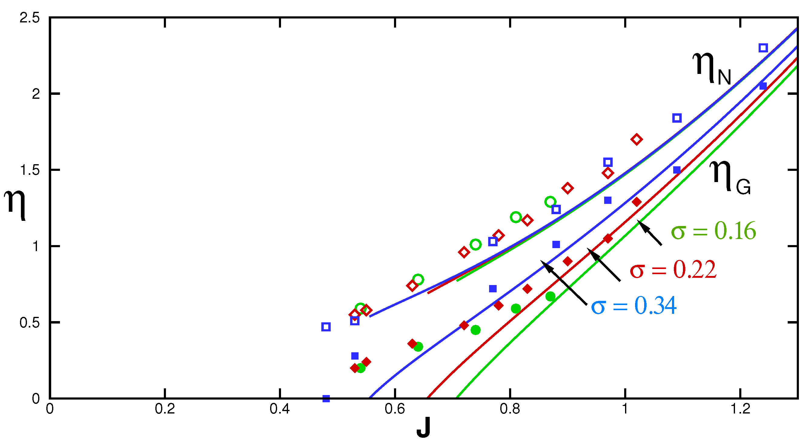
The box-model predictions for the tested flows are straightforward. For the AXI system with , we obtain , (see (27)) and (33)). For a given , the algebraic equation (34) and (40) provide values of and for various J of interest. Using these results and the conversion , we present in Figure 11 a similar plot to Fig. 4 of [7]. The the lines are box-model predictions. There is a fair agreement of the predictions with the data. We see that the model predicts correctly the behaviors of and . There is strong decay of as J decreases from 1.2 to 0.5 (approximately). However, the effect of on this variable is remarkably small: the theoretical lines for the three values of almost overlap, and the open symbols for the three values of collapse on a smooth (imaginary) line. decreases faster than as J decreases. increases with , as seen in the prediction lines and in the filled symbols. (For the comparison with data is irrelevant because the GC is unconfined.)
The box model provides the physical interpretation of these trends. The parameter J is proportional to . When the influx rate decreases and/or the gap increases, the parameter J decreases, and in the physical system the coefficients and of the propagation of the fronts, see (46), are expected to decrease due to volume conservation. A larger cause a smaller effective thickness , see Figure 1(b), and a smaller buoyancy force . This allows a reduction of the bottom drag of the GC which is . Consequently, at a fixed J, a larger appears for a larger . The behaviour of is subtle. For a fixed J (fixed influx) a larger renders a smaller effective thickness ; this would suggest an increase of to accommodate the volume. Here enters the second front. The larger increases , which means an increase of the radius of the slug. The larger slug absorbs a larger portion of the influxed fluid, and counteracts the expected increase of . The resulting flow displays a value of which is little affected by the variations of in these data.
The quantitative discrepancies between the data and the theoretical predictions observed in our Figure 11 are, roughly, of the same magnitude for the present box model and the lubrication model used by [7] (Fig. 4 in that paper). It is not possible to determine how much of the discrepancy is attributable to the box-model simplifications, because of the restricted data set, experimental errors, and uncertainty of the parameter . Taking into account the fact that the box model predicts correctly the values of and of the experimental system, the overall predictions of the box model in this test seem to capture well the physical balances of the flow under consideration. In our opinion, this comparison provides support to the box-model as a predictive tool for realistic systems, and motivates further tests in other systems, in particular power-law fluids.
5. Conclusions
We presented a box-model analysis of the flow of a viscous fluid injected into a horizontal gap of height H in rectangular 2D and cylindrical AXI geometries, for a power-law non-Newtonian fluid (). When the displaced (ambient) fluid is less dense and significantly less viscous than the injected one (a typical occurrence in molding industry), and the influx is sufficiently strong, the leading part of the flow is a GC while the tail fills the gap. We focused attention on the influxed volume . We showed that for certain values of (depending on n) the flow is self-similar: the propagation of the nose and of the grounding line are like and . In general, in 2D and in AXI. We recall that the unconfined GCs display self-similar propagation for any . The confinement restricts the similarity flow to and in 2D and AXI flows, respectively. We obtained explicit formulas for the stringent features of the flow field, like . All the results are in good agreement with the more rigorous lubrication-model solution (which does not assume a horizontal interface). In particular, we note identical prediction for the time-power coefficients and , and a surprisingly small discrepancy for the dimensionless prefactor .
In general, the flow under consideration depends on four parameters: and . The box-model demonstrates that the dependencies are strongly coupled and non-linear, and hence a simple model is helpful for understanding the physical influence of each of the parameters.
The box model reveals that the main surface tension effects, , are: (a) for a fixed J, the position increases; and (b) for maintaining a fixed , J must be reduced. The effects of a nose meniscus are in the same direction, but .
The restriction of the solution to special values of the influxed volume coefficient reproduces a physical condition, not a mathematical simplification. We argue that the similarity behaviour corresponding to this is essential in the present problem; influx with a different is bound to produce a very different flow pattern. The present keeps the grounding line between the inlet and the nose (). In this case the GC elongates, but maintains a constant average thickness. When is reduced, the GC tends to become thinner with t, the grounding line moves toward the inlet, and an unconfined GC appears on the bottom of the gap. When is increased, the GC tends to become thicker with t, the grounding line moves toward the nose, and all the injected fluid behaves like a slug in contact with both boundaries of the gap. It is remarkable that the similarity solution is robust: for a given geometry, the time powers and depend on n, and are unaffected by the presence of surface tension effects represented by and . This interesting prediction has been verified experimentally for the AXI system and ([7]), and further tests will be beneficial.
We recall that the accurate value of the surface-tension parameter is not available for practical systems. The comparisons of predictions with data, performed by [7] and here in § Section 4, suggests that is a fair approximation. This is a good starting point for the practical use of the present models. However, we must keep in mind that the data set of [7] covers only AXI flow of a Newtonian fluid. For the assessment and improvement of the extended theory, a much wider experimental study is necessary. We hope that this will be reported in the near future.
The advantage of the box model is in the simplicity of the derivation and the predictions. We straightforwardly gain the insight that the kinematic (volume continuity) balances determine the relation between and , and the coefficient K; the dynamic force balance determine the values of and . The interconnections between the dimensionless variables are expressed in explicit formulas, without any adjustable constants. The description of the flow has been reduced to a set of basic algebraic-substitution formulas. The influence of the surface tension meniscus at the grounding line (parameter ) is well elucidated. The box model also clarifies that the effect of the nose meniscus (parameter ) is typically negligible. These simplifications are expected to facilitate the analysis and design of various applications. Needless to say, the same information can be extracted from the more rigorous lubrication model, but this requires a more significant effort of programming, data processing, and interpretation.
We emphasize that, in general, the box model is an unreliable prediction tool, unless subjected to stringent verification against some more accurate results over a significant range of parameters. The present box model can be recommended because it has passed such tests (without using any adjustable constants), and we have reliable information about the expected error concerning the sign (under/over prediction) and order of magnitude. However, we keep in mind that this paper compares mostly between two theories based on simplifications (such as thin layer, hydrostatic pressure, sharp meniscus, well-controlled influx). The convincing assessment of the models requires critical comparison with experimental data. (The comparison with the data of [7] is in § Section 4 is encouraging, but covers a restricted domain, in particular .) In view of the large number of involved parameters, this is a challenging experimental task. We are confident that the present quite sharp theoretical predictions will facilitate the experimental verification.
Appendix A. The Effect of the Nose Meniscus
We assume that the height of the nose meniscus is . The surface tension of this meniscus yields a drag force on the GC. We estimate this force, , from the observation that the meniscus truncates the sharp tip of the GC shown in Figure 1(a). The lubrication balance in this region (before truncation, with no surface tension) is
where is the viscous stress in the fluid. Suppose that the truncation is from position where to position where . Integration of (A1) with respect to z and then x (with the appropriate boundary conditions) yields the connection between the height and the friction force of the tip section
After that truncation, point M is considered to be the nose (N) affected by the meniscus. We return to the box model. Letting , we therefore estimate that the drag force of the nose meniscus is (for 2D). This force is conveniently subtracted from the buoyancy force of the original box model. Consequently, we estimate that the buoyancy available for counteracting the bottom shear is reduced to in 2D (multiplied by in AXI).
The incorporation of this effect in the foregoing analysis requires a simple modification: use instead of . The box model indicates that the effect of (the nose meniscus) is (a) in the same direction as that of , but (b) much smaller than that of (the grounding line meniscus). The details are as follows.
We note that now the RHS of (16) and (34), which govern the position , will be multiplied by . Using these balances and an expansions in powers of , we estimate the changes of the basic flow () due to a small . We obtain:
For 2D.
Suppose that the surface tension imposes some small . Comparison of (A5)–(A6) with (21), (22), (38) and (39) demonstrates that the contribution of the grounding-line meniscus (represented by the parameter ) is consistently much more significant. These box-model estimates are in agreement with the lubrication-model tests of [7]. We have also performed lubrication-model tests with (details not shown) and detected small variations.
The conclusion is that the for the confined GC the dominant surface tension effect is at the grounding line.
Appendix B. The Lubrication Model
The lubrication model for power-law viscous GCs with no surface tension () in 2D and AXI geometries is presented in U25. Equations of that paper will be denoted by the addition of U in the number. Here we briefly describe the modifications when non-zero and/or are present. Physically, the menisci at the grounding line and/or nose are assumed to be vertical jumps of the interface which do not affect the mechanics of the GC. The governing equations of the GC are unchanged, but the boundary conditions at and/or at (the nose) must be modified.
Consider the GC of Figure 1(a). We use dimensionless variables scaled according to (23) (see also (4.6U) ), but in this appendix we drop the upper ∼ (in particular, K here corresponds to in the main text). The dimensionless height of the gap is 1.
The continuity equations are
Let denote x or r. In the GC, the depth-averaged velocity is .
Let The boundary conditions at the nose are while . These conditions are not affected by the meniscus at the grounding line.
For 2D. The grounding line poses two conditions for the GC at . First, the obvious . Second, the total volume conservation
We apply t derivative to the balance (A8), use (A7) to eliminate , and recall . We obtain the flux condition at
For AXI. The boundary conditions at the grounding line is the obvious and the total volume conservation (per radian) which reads
The governing lubrication-model equations for the GC, (4.6U)–(4.9U) and (4.11U)–(4.12U), are not affected by the presence of the meniscus. The only difference is the change of the boundary condition at (or ) when : instead of (4.10aU) and (4.10bU) we should impose (A9) and (A11).
The lubrication model postulates the similarity solution
where y is the reduced length coordinate, . It can be verified that the new flux conditions are compatible with these similarity assumptions when in 2D case (or in AXI case).
The conclusion is that the similarity solution of the lubrication model for the confined GC in the system developed in U25 can be extended to the system with (at this stage, without a nose meniscus). For a given n, the values of the time-powers and are unchanged, and in full agreement with the box-model predictions ((9) and (15) for 2D, (27) and (33) for AXI). The definition and meaning of the parameter J is unchanged, in full agreement with the box model. The new parameter will affect the values of J and K for a given .
The height profile of the interface of the GC can be calculated by the same method as described in U25 (in particular using (4.16U)–(4.21U)). To be specific, the major equation is
subject to the values of and at , for a small , obtained from the approximation
In other words, when , for a given n and geometry, is a universal profile for . We obtain and by numerical integration of (A13). This part of the solution process is independent of the value of , and thus exactly as described in U25.
The calculation of J and K for a given is affected by . At the position , where and are known, the new grounding-line conditions (of height and volume flux) yield
where for 2D and 3 for AXI. For given n, and we obtain the values of J and K of the confined GC. For we recover the results of U25. The results of [8] and [7] are recovered for and AXI geometry (but note that these papers use a different scaling of the variables).
Equation (A16) indicates that in 2D case, and in AXI case. These dependencies are in agreement with the box-model predictions (24) and (40). However, it is evident that the box model formulas are simpler and more insightful. (Recall that K in this appendix corresponds to in the main text.)
A nose meniscus can be implemented as follows. Assume that the height (dimensionless) is . (Note that of Appendix A multiplies of the box model. Hence .) The relevant conditions at are and . The differential equation for and the flux condition at the grounding line are not affected (the derivation of (A9) and (A11) is slightly modified because ). When , the condition for and applied at according to (A14) must be changed to
Equation (A18) expresses the condition . The similarity solution calculation of is now implicit, because the unknown K appears at and , see (A17) and (A15). is no longer a universal profile. An iteration is needed, such as: for a given , guess an initial K, use (A17)–(A18) to solve the equation from to , calculate the new K by (A15), repeat the solution with a corrected K, until convergence of K is achieved. Then calculate J by (A16). This iteration complicates the solution, but since the effect of is very small, the simpler solution without the nose meniscus is in general a sufficiently accurate prediction.
We used a Runge-Kutta method for the calculation of .
The present extension of the similarity solution of the basic lubrication-theory model (without surface tension effects) to GCs affected by surface-tension effects has been facilitated by the assumptions that the menisci lengths are fixed with respect to a geometric scale, H, present in the previous formulation. A more realistic modeling of the menisci may introduce a new lengthscale and require a more complex solution of the interface. This topic is left for future work.
Acknowledgments
We thank prof. A.J. Hutchinson for help concerning the experimental data used in § Section 4.
Conflicts of Interest
The author reports no conflict of interests.
| 1 | The force balance for the slug is unimportant in the present analysis. We assume that the source (pump) at provides the pressure necessary for sustaining the flow of the influxed fluid in the gap . |
References
- Chowdhury, M. R. & Testik, F. 2011 Laboratory testing of mathematical models for high-concentration fluid mud turbidity currents. Ocean Eng. 38, 256–270. [CrossRef]
- Ciriello, V. & Di Federico, V. 2013 Analysis of a benchmark solution for non-newtonian radial displacement in porous media. Int. J. of Non-Linear Mech. 52, 46–57.
- Didden, N. & Maxworthy, T. 1982 The viscous spreading of plane and axisymmetric gravity currents. J. Fluid Mech. 121, 27–42. [CrossRef]
- Hinton, E. M. 2020 Axisymmetric viscous flow between two horizontal plates. Phys. Fluids 32 (6), 063104.
- Hoffman, D. A. 2014 Understanding the gravity of the situation. Plastics Eng. 70 (10), 28–31. [CrossRef]
- Huppert, H. E. 1982 The propagation of two-dimensional and axisymmetric viscous gravity currents over a rigid horizontal surface. J. Fluid Mech. 121, 43–58. [CrossRef]
- Hutchinson, A. 2024 The effect of surface tension on axisymmetric confined viscous gravity currents. Partial Differential Equations in Applied Mathematics 12, 100992. [CrossRef]
- Hutchinson, A., Gusinow, R. J. & Grae Worster, M. 2023 The evolution of a viscous gravity current in a confined geometry. J. Fluid Mech. 959, A4–1–13. [CrossRef]
- Longo, S., Di Federico, V., Archetti, R., Chiapponi, L., Ciriello, V. & Ungarish, M. 2013 On the axisymmetric spreading of non-Newtonian power-law gravity currents of time-dependent volume: an experimental and theoretical investigation focused on the inference of rheological parameters. J. non-Newtonian Fluid Mech. 201, 69–79.
- Taghavi, S. M., Seon, T., Martinez, D. M. & Frigaard, i. a. 2009 Buoyancy-dominated displacement flows in near-horizontal channels: the viscous limit. J. Fluid Mech. 639, 1–35.
- Ungarish, M. 2020 Gravity Currents and Intrusions — Analysis and Prediction. World Scientific, New Jersey, London, Tokyo.
- Ungarish, M. 2025a Improved box models for Newtonian and power-law viscous gravity currents in rectangular and axisymmetric geometries. Fluids 10,207, 1–18.
- Ungarish, M. 2025b The self-similar flow of Newtonian and power-law viscous gravity currents in a confined gap in rectangular and axisymmetric geometries. J. Fluid Mech. 1007, A4–1–24, referred to as U25. [CrossRef]
- Zheng, Z., Rongy, L. & Stone, H. A. 2015 Viscous fluid injection into a confined channel. Phys. Fluids 27 (6), 062105. [CrossRef]
- Zheng, Z. & Stone, H. A. 2022 The influence of boundaries on gravity currents and thin films: Drainage, confinement, convergence, and deformation effects. An. Rev. Fluid Mech. 54, 27–56. [CrossRef]
Figure 1.
Sketch of the confined system: (a) lubrication model for the GC with inclined interface, and (b) box model with horizontal interface . The height of the meniscus at the grounding line is . The volume (per unit width) is . In the self similar flow, , , and depends on the parameter J. In the axisymmetric geometry, r replaces x and is per radian. are constants.
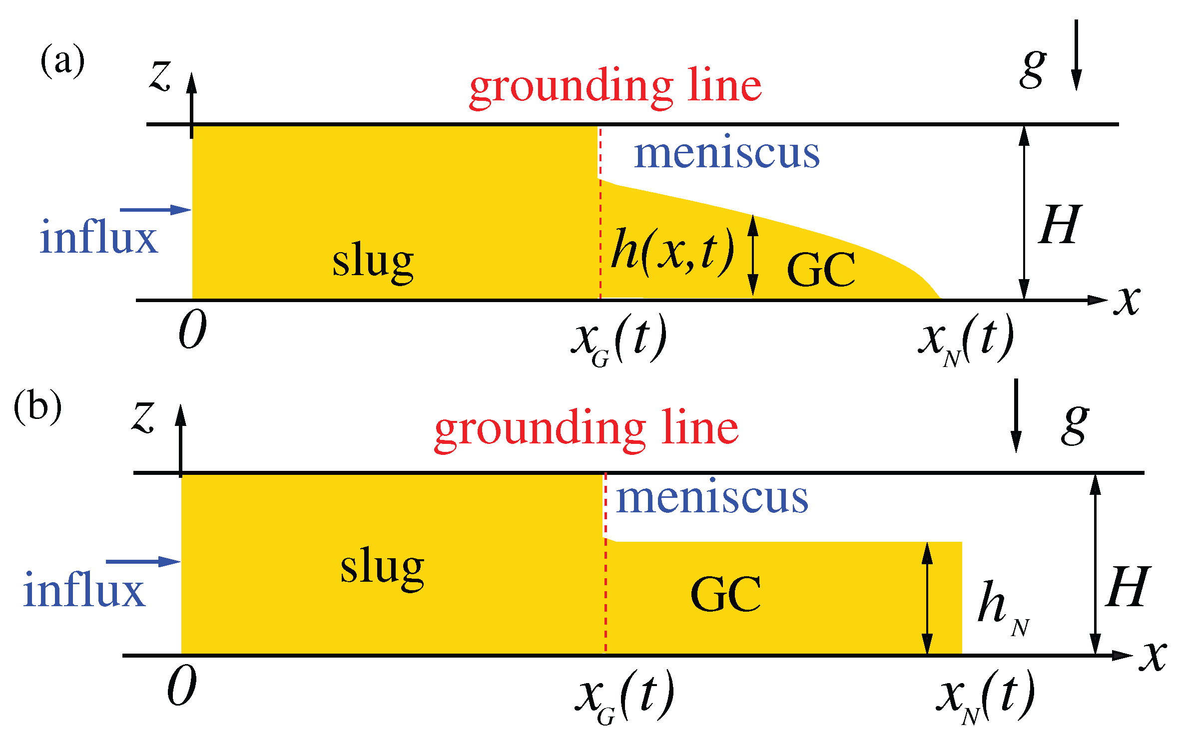
Figure 2.
2D case. The slopes and as functions of for various n.
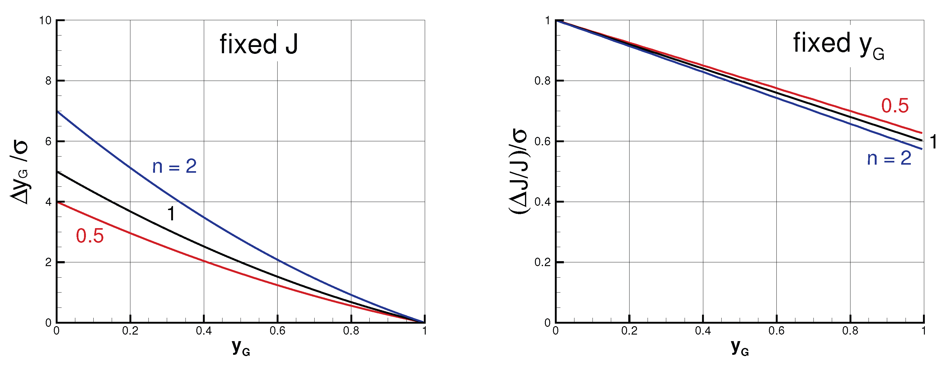
Figure 3.
Box model (dash-dot line) and lubrication model (solid line) results J vs. yG. for σ = 0 (black lines) and σ = 5 and (red lines) for 2D system. The frames are for n = 0.5, 1, 2.
Figure 3.
Box model (dash-dot line) and lubrication model (solid line) results J vs. yG. for σ = 0 (black lines) and σ = 5 and (red lines) for 2D system. The frames are for n = 0.5, 1, 2.
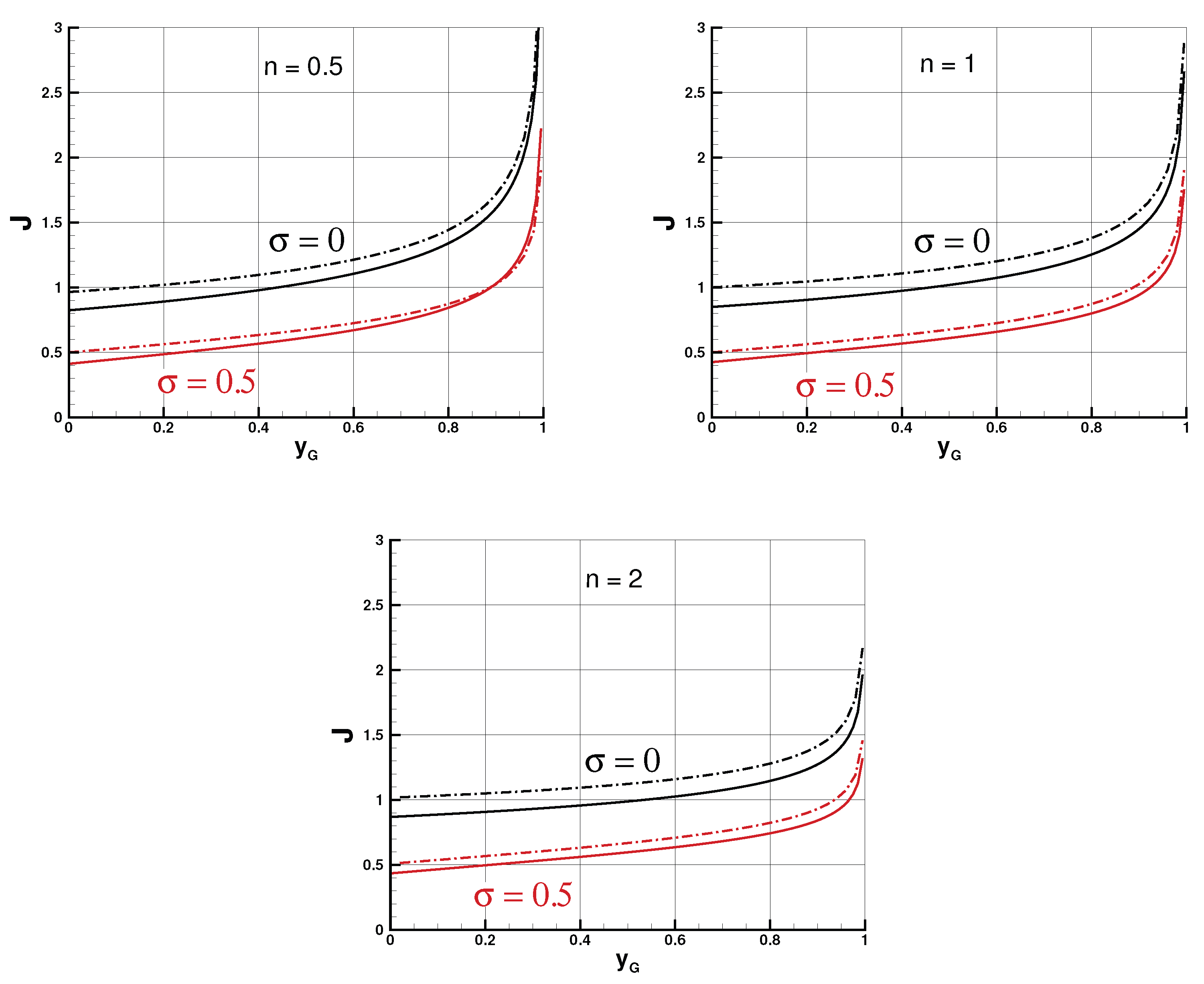
Figure 4.
vs. J for the systems of previous figure.
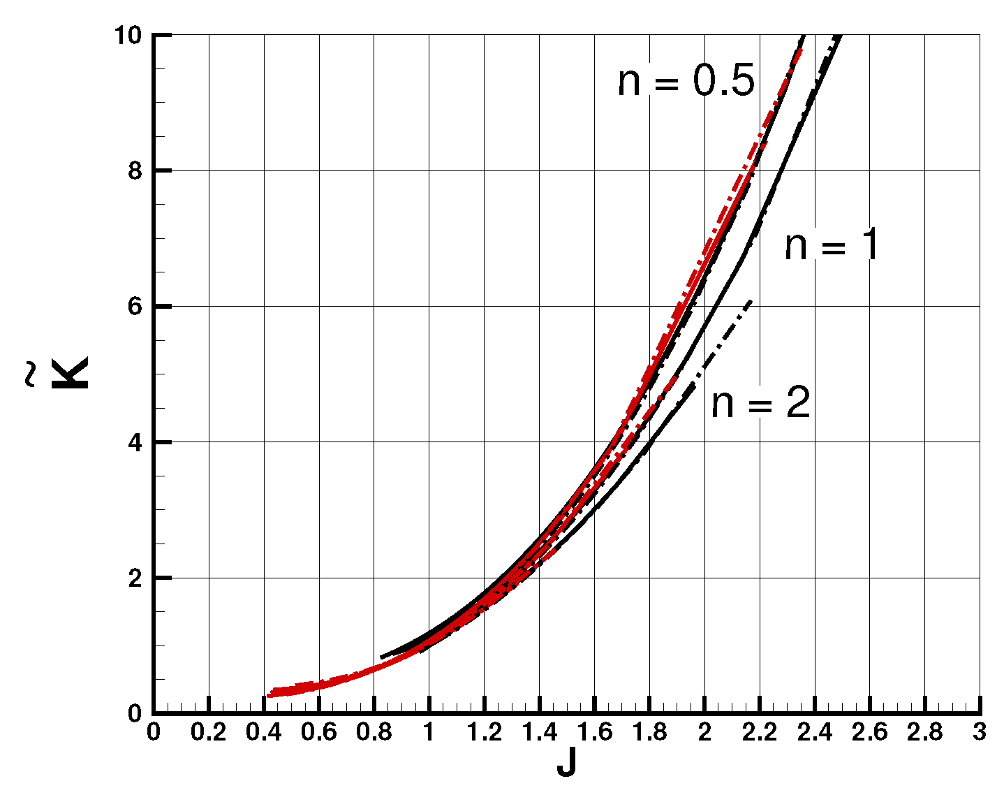
Figure 5.
AXI case. The slopes and as functions of for various n.
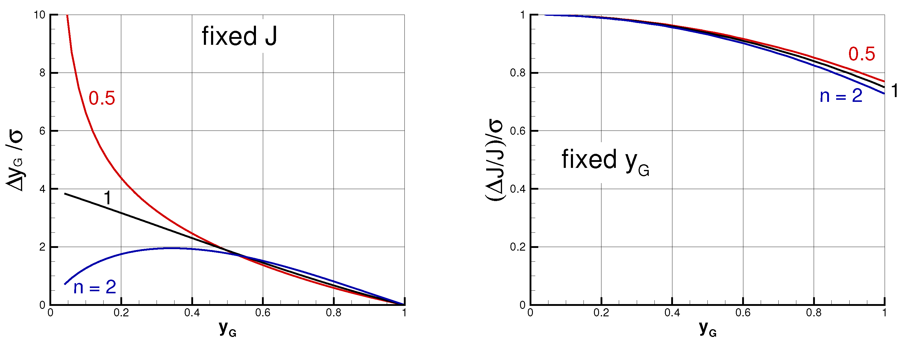
Figure 6.
Box model (dash-dot line) and lubrication model (solid line) results J vs. yG. for σ = 0 (black lines) and σ = 5 and (red lines) for AXI system. The frames are for n = 0.5, 1, 2.
Figure 6.
Box model (dash-dot line) and lubrication model (solid line) results J vs. yG. for σ = 0 (black lines) and σ = 5 and (red lines) for AXI system. The frames are for n = 0.5, 1, 2.
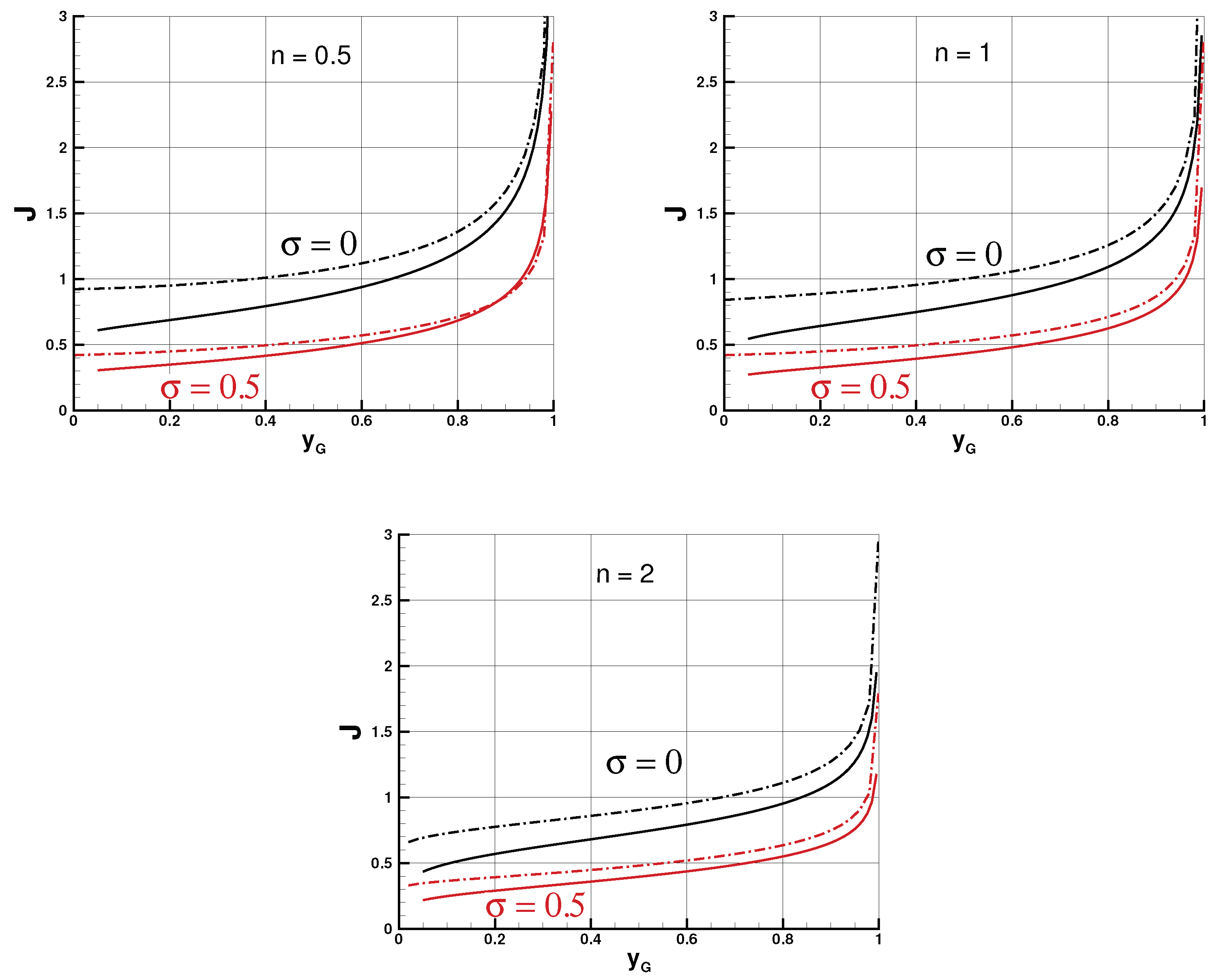
Figure 7.
vs. J for the systems of previous figure.
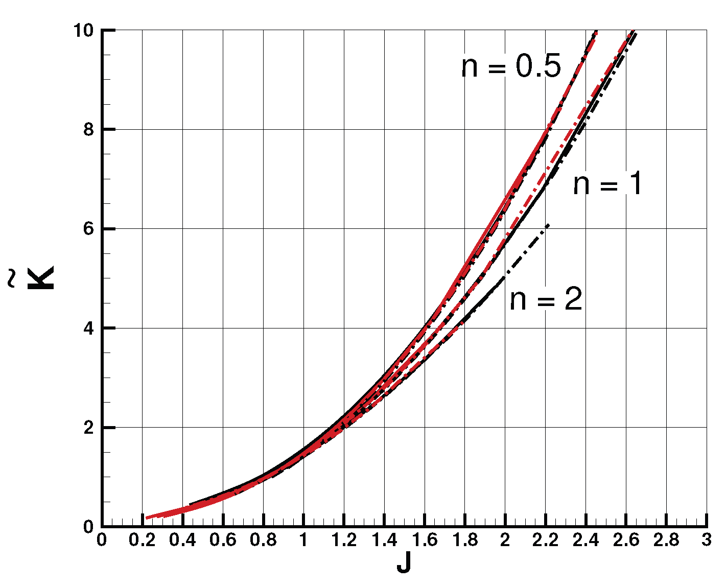
Figure 8.
Box model (dash-dot line) and lubrication model (solid line) results for 2D system for . (a,b) J and as functions of for various n (0.5, black; 1, red, 2, green). (c,d) as functions of n.
Figure 8.
Box model (dash-dot line) and lubrication model (solid line) results for 2D system for . (a,b) J and as functions of for various n (0.5, black; 1, red, 2, green). (c,d) as functions of n.
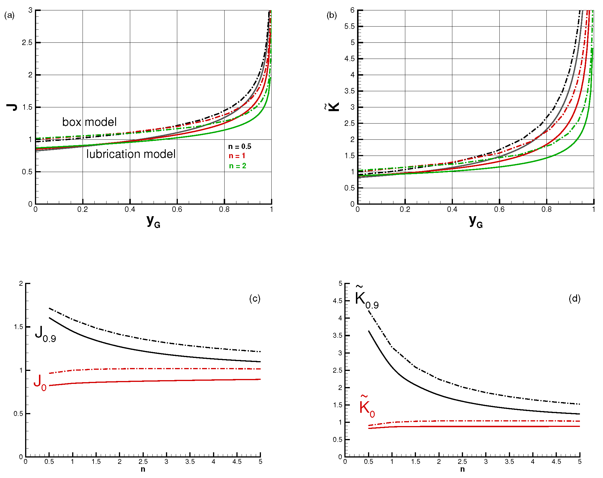
Figure 9.
vs. J for , various n. Box model (dash-dot line) and lubrication model (solid line). (a) 2D and (b) AXI system. The red and green lines end at the value of J for which .
Figure 9.
vs. J for , various n. Box model (dash-dot line) and lubrication model (solid line). (a) 2D and (b) AXI system. The red and green lines end at the value of J for which .
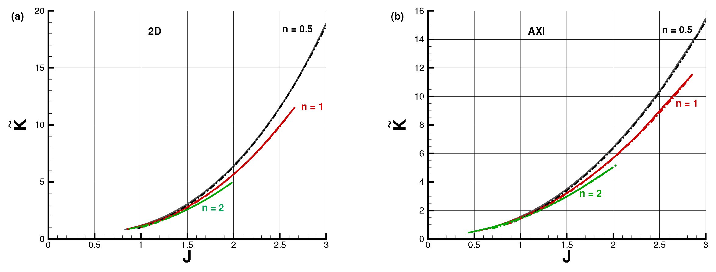
Figure 10.
Box model (dash-dot line) and lubrication model (solid line) results for AXI system for . (a,b) J and as functions of for various n. (c,d) as functions of n.
Figure 10.
Box model (dash-dot line) and lubrication model (solid line) results for AXI system for . (a,b) J and as functions of for various n. (c,d) as functions of n.
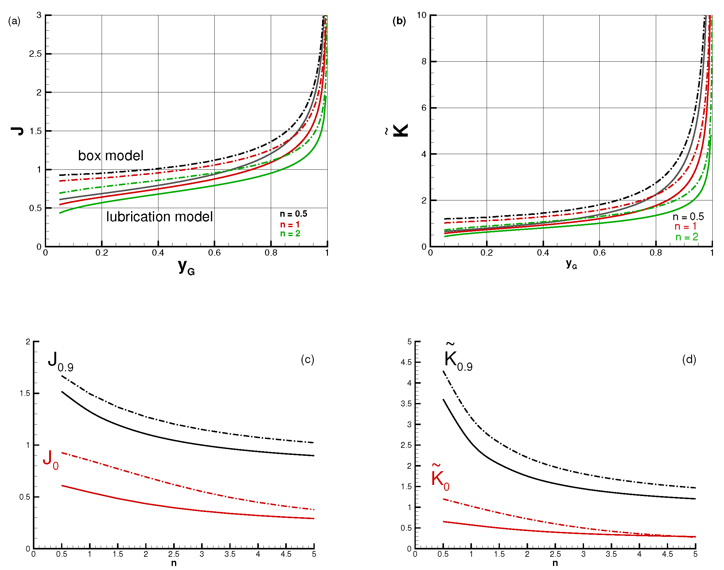
Figure 11.
and as functions of J for (green, red, blue). Box model (lines) and data of [7] (open symbols for , filled symbols for ). (For the GCs are typically unconfined, and outside the scope of our model.)
Figure 11.
and as functions of J for (green, red, blue). Box model (lines) and data of [7] (open symbols for , filled symbols for ). (For the GCs are typically unconfined, and outside the scope of our model.)
Disclaimer/Publisher’s Note: The statements, opinions and data contained in all publications are solely those of the individual author(s) and contributor(s) and not of MDPI and/or the editor(s). MDPI and/or the editor(s) disclaim responsibility for any injury to people or property resulting from any ideas, methods, instructions or products referred to in the content. |
© 2025 by the authors. Licensee MDPI, Basel, Switzerland. This article is an open access article distributed under the terms and conditions of the Creative Commons Attribution (CC BY) license (http://creativecommons.org/licenses/by/4.0/).
Copyright: This open access article is published under a Creative Commons CC BY 4.0 license, which permit the free download, distribution, and reuse, provided that the author and preprint are cited in any reuse.


