
Submitted:
17 September 2025
Posted:
22 September 2025
You are already at the latest version
Abstract
Background: Noise is one of the externalities of transportation systems in cities. To help understand which neighborhoods have noise levels exceeding the World Health Organization’s (WHO) thresholds, scholars have proposed the use of spatial noise maps. Most cities in developed nations have regularly produced these maps. Unfortunately, in developing nations, citizens still lack this important tool to help in the identification of quieter neighborhoods. One such, is Nairobi, the capital city of Kenya hence the reason for this study. In previous studies, varying methods have been used to produce Road Traffic Noise maps, such as Inverse Distance Weighting (IDW), Ordinary Kriging (OK), among others, each of which has its pros and cons. Aims: This study aimed to develop a GIS-based spatial model of Road Traffic Noise distribution in Nairobi city in Kenya. This was motivated by the fact that the ambient environmental conditions of urban neighborhoods are an indicator of how the welfare of their residents is taken care of. Study Design: This study deployed the GIS-based IDW method. Place and Duration of Study: The Department of Civil and Construction Engineering, University of Nairobi coordinated data collection across the city, between 6th July, 2025 and 12th July, 2025. Methodology: A seven-day Road Traffic Noise data for twelve hours from 6 AM to 6 PM using a handheld Class 1 Sound Level Meter was collected. The data was then bundled into two-hour intervals, resulting in six map presentations. GIS-based spatial maps were then subsequently produced using IDW method. Results: According to the maps, the noisiest time falls between 12 PM and 2 PM, while the low-noise periods occur from 8 AM to 10 AM and from 4 PM to 6 PM. Inferentially, noisy road corridors have high speed in the periods mentioned, and quieter corridors are heavily congested over the same time period. Notorious noisy road corridors in Nairobi include Ngong Road, Waiyaki Way, Eastleigh area, and Thika Road, and the quieter neighborhoods are in Runda and Karen areas. Conclusion: This study concludes that the GIS-based noise maps are helpful tools for residents to choose areas of habitation with a tolerable soundscape and to make noise management sustainable, by deploying GIS-based real-time noise maps accessible via the internet web display.
Keywords:
road traffic noise
; map
; hotspot
; spatial modelling
1. Introduction
The developing city intersection conforms in many ways to a hazardous area for noise pollution. In under-developed cities, often the city builds around road intersections. Intersections of national highways, state highways, or two-state highways are the prime areas around which a city builds up. The roads and crossroads (intersections) are associated with less control over traffic and multiple vehicles of varying speeds frequently run at similar times on the roads. The congestions at city intersections keep on increasing with growing establishments around the intersections. The authorities of several such unplanned cities also allow the establishment of schools, health centers, shops, sports centers, roadside open markets, etc. around the intersections, which results congestion (Zafar et al., 2023; Zhou et al., 2024). Noise is the unwanted or harmful sound that interferes with people’s day-to-day activities, such as communication, business, and rest. It also causes adverse effects on physical and mental well-being. Noise is fleeting, and it completely vanishes or diminishes when the source is controlled, and its impact can trigger physiological and psychological responses ranging from annoyance and sleep disturbance to health risks such as cardiovascular diseases and impaired cognitive functions, as well as reduced quality of life (Basner et al., 2014; Münzel et al., 2018).
One of the most dominant forms of noise pollution in urban environments is Road Traffic Noise (RTN). Arguably, it is listed among the most pervasive forms of environmental pollution in urban soundscapes ecosystems, often exceeding the recommended exposure limits by the World Health Organisation (WHO) standards, especially in densely populated cities with high vehicle traffic volumes (Basner et al., 2014). In the developing countries, the rapid urban development and increase in vehicular volume have amplified the RTN levels, exacerbating concerns over overall community health, environmental degradation, and the quality of life (Garg et al., 2017). Measuring traffic noise levels and representing them spatially using Geographic Information System (GIS) maps offers a powerful tool for identifying noise sources, analyzing their spread, and implementing effective control measures. Road traffic noise is a major contributor to environmental pollution in urban settings (Singh & Jha, 2023).
Measurement of RTN is an important step in understanding its impact and developing targeted noise mitigation and abatement strategies. Numerous studies have been done to assess the RTN levels and their impact in both developed and developing nations’ cities. For example, in Tokat, Turkey, Ozer et al. (2009) measured RTN levels, in which they established that RTN levels exceeded the set national limits. Similarly, in Varanasi City, India, Pathak et al. (2008) found an alarming RTN level, with the majority of the city residents reporting disturbance and annoyances. Further, in Cáceres, Spain, Morillas et al. (2002) studied and examined urban noise and also identified road traffic as the most prevalent source of noise pollution. Such studies have underscored the importance of RTN-based measurement to inform urban planning and targeted mitigation and abatement strategies.
Although direct measurement of RTN provides useful information on point-specific data, the geographical variability and temporal patterns of RTN exposure across urban environments are not fully captured by these readings. Noise mapping has emerged as an essential tool for evaluating and visualizing spatial variations in environmental noise levels. It transforms discrete data into continuous spatial representations, providing a baseline for urban authorities to identify major noise hotspots, inform policies, and employ mitigation strategies. The best to guide all these actions is noise maps, which are outputs of interpolated RTN data 2-dimensional plane display.
A noise map is defined as a graphical representation that shows the noise distribution across a geographically defined area. It integrates acoustic data with spatial coordinates (Murphy & King, 2014) to show how noise levels vary across an area. Numerous studies have employed noise mapping in their research. For instance, Murphy and King (2010) produced detailed RTN maps for Dublin, Ireland, to support compliance monitoring under the EU Environmental Noise Directive (END). In the same breadth, (İlgürel et al.,2016) used simulation and GIS-based modeling to create RTN maps to show the levels in Istanbul, Turkey. Recently, Esmeray and Eren (2021), while studying the situation of noise in Safranbolu, Turkey, were able to develop a GIS-based noise map to visualize the spatial distribution of noise hotspots across the city. In India, Partheeban et al. (2022) studied the busy corridors of Chennai and while Dey et al. (2021) did for Mumbai. The two team both applied spatial mapping in their studies to demonstrate how strategic noise mapping is useful in identifying urban areas with critical noise exposure levels as well as to isolate graphically the major noise hotspots.
Production of accurate noise maps relies on spatial interpolation, a process by which the values of variable locations, where no measurements have been taken, are estimated based on the known values from surrounding locations. There are several spatial interpolation methods available for environmental mapping, including Ordinary Kriging (OK), Radial Basis Function (RBF), Empirical Bayes Kriging (EBK), Local Polynomial Interpolation (LPI), and Inverse Distance Weighting (IDW). Each of these methods has its pros and cons (Bhunia, et al., 2018; İmamoglu & Sertel, 2016; Boumpoulis, et al., 2023; Arseni et al., 2019). In addition to these methods, Machine Learning approaches such as Neural Networks and Random Forests have also been explored for spatial interpolation. (Bélisle et al., 2015).
Ordinary Kriging (OK) is a geostatistical interpolation technique that employs semivariogram models to measure the spatial autocorrelation and provide the Best Linear Unbiased Estimates (BLUE) when a spatial structure is well characterized (İmamoglu & Sertel, 2016). It estimates prediction uncertainty while handling data that is unevenly distributed. However, OK is computationally intensive and data sensitive, producing incorrect findings, especially when there is insufficient data or weak spatial structures (İmamoglu & Sertel, 2016; Bhunia, et al., 2018). On the other hand, the Radial Basis Function (RBF) interpolation method employs mathematical functions like thin-plate splines, multiquadrics, or Gaussian functions to generate a smooth surface-fitting method by estimating values that adapt well to complicated gradients. However, the choice of the basis function and its parameters has a significant impact on the results. In highly variable noise environments, RBF may cause over-smoothing (Arseni et al., 2019).
Another OK method is the classic Kriging technique, which is a form of improved Empirical Bayes Kriging (EBK) method. It accounts for uncertainty in its estimates by automating variogram modelling using an iterative simulation-based methodology. By automating variogram modeling with an iterative simulation-based methodology, it takes uncertainty in its estimations into account. Because EBK automatically estimates the variogram parameters from the data, it is particularly helpful when the dataset is too small for traditional variogram modeling or when the underlying spatial structure is complex (Arseni et al., 2019). This method has improved the accuracy, though it requires high computational capacity (İmamoglu & Sertel, 2016). Local Polynomial Interpolation (LPI) fits a polynomial function to portions of the data to estimate values at unknown sites. It is comparatively robust to extreme values and catches slow patterns in the data. In noise mapping, when sudden changes are frequent, it could be crucial to smooth out acute local fluctuations (Bhunia, et al., 2018). Although it might not be as accurate at fine scales, it is helpful in situations with non-stationary patterns.
Inverse Distance Weighting (IDW) is a deterministic method that estimates unknown values at specific locations based on the values of known locations by assigning higher weights to points that are closer to the prediction location and lower weights to those farther away. The weighting exponent (denoted as p) controls the influence of distance on the interpolation. A higher p-value increases the influence of nearby points while reducing the effect of distant ones, resulting in more localized predictions, whereas lower values produce smoother surfaces. It is computationally straightforward and does not require complex statistical modeling. It is, however, sensitive to clustering, potentially overemphasizing local anomalies (Bhunia et al., 2018). In addition to these methods, Machine Learning approaches, including Artificial Neural Networks (ANNs) and Random Forests, have emerged as a technique for spatial interpolation in recent years. These methods may combine several predictor factors outside of geographical coordinates, such as traffic volume and weather conditions, and model extremely nonlinear connections. They are computationally demanding, need big datasets, and have the potential to overfit data, even if they can outperform traditional interpolation methods (Bélisle et al., 2015).
Out of all the spatial interpolation techniques, Inverse Distance Weighting (IDW) has gained traction as the most appealing technique for urban RTN mapping. It is computationally straightforward, is easily interpretable, and suitable for datasets with moderate measurement density and relatively uniform geographical distribution, and situations where resources or technological capability restrict the application of more complex geostatistical methods. The IDW interpolation approach has been successfully used to create noise maps in a number of studies. Thanh and Hạnh (2021) used IDW to map the urban noise of Thuan An City, Vietnam; Islam et al. (2024) evaluated RTN and possible public health risks in Barisal, Bangladesh; and Jalilzadeh (2007) evaluated noise pollution in Tehran, Iran. In Sub-Saharan Africa, RTN has emerged as a significant environmental health challenge driven by rapid urbanization, an increase in population, and a surge in vehicular traffic. Development of infrastructure, coupled with improper or inadequate noise regulation enforcement, has resulted in elevated noise exposure levels among city residents. Unlike other developing countries worldwide, most Sub-Saharan African cities lack proper research on RTN with spatially detailed noise maps for visualization, limiting the ability to implement targeted interventions.
Nairobi, the capital city of Kenya, is one of the most rapidly urbanizing cities in Eastern Africa. It is characterized by a growing population, dynamic economic activities, a mixed land use pattern, and busy transport corridors that serve both local and regional mobility needs. These factors, combined with surging vehicular traffic and inadequate or improper noise abatement strategies, contribute to the growing RTN problem. Although environmental noise has emerged as a notable public health and urban planning concern, systematic, citywide RTN assessments in Nairobi still remain a huge knowledge gap. Previous geospatial studies of environmental noise phenomena in Nairobi city have demonstrated the value of spatial noise pollution modeling which calls attention to the need for urban noise management. Notably, previous efforts are the work by Wawa and Mulaku (2015) FF who applied Geographic Information System (GIS) in Nairobi’s Central Business District to produce the first-ever noise map, showing the average recorded noise levels. Their research illustrates how spatial interpolation methods can provide urban authorities with actionable and location-specific insights. Such approaches have rarely been applied comprehensively to traffic noise in Nairobi. Building on these methodological foundations, this study employs the Inverse Distance Weighting (IDW) interpolation technique within a GIS framework to generate high-resolution RTN maps based on measured equivalent continuous sound level (Leq) values from 42 selected sites. The resulting maps will enable identification of noise hotspots, inform targeted policy interventions, and contribute to the emerging discourse on sustainable urban soundscapes in rapidly urbanizing cities.
2. Material and Methods
2.1. Study Area and Site Selection
The study was conducted in Nairobi city, the capital of Kenya, see Figure 1, and the largest urban center in the country, geographically lying between a latitude of 1° 09′ and 1° 27′ South, a longitude of 35° 59′ and 37° 57′ East.
Nairobi covers an area of approximately 696 km², characterized by a diverse mix of commercial, industrial, residential, and green spaces. As Kenya’s political, economic, and transport hub, Nairobi experiences high volumes of vehicular traffic, resulting in elevated levels of RTN. From a radius of 14km from the city center, 42 sampling points were selected to measure the RTN levels. The coordinates of these points were geolocated and mapped using ArcGIS, see Figure 2.
2.2. Data Acquisition
The coordinates of each of those 42 measurement points were first confirmed by Google Maps, a Global Positioning System (GPS) application. Using a factory calibrated Class 1 Lutron SL-4033SD Sound Level Meter, conforming to IEC 61672-1 standards, see Figure 3, RTN measurements were carried out at each of these selected sites for 7 days.
For each day, measurements were carried out at hourly intervals for fifteen minutes each hour. The SLM was handheld and placed at an approximate height of 1.5 meters from the ground to minimize reflections and direct influence from passing vehicles. They were oriented towards the traffic flow to ensure direct exposure to incident sound waves, see Figure 4.
The SLM was set in fast response mode, which is ideal for recording the quickly varying nature of RTN. To account for the human ear's response to sound, an A-weighting filter setting was used. To ensure high resolution, data were logged at 2-second intervals on an Excel file during each 15-minute sampling session, enabling the computation of the equivalent sound pressure level (Leq) using the formula:
Where
represents each SPL reading taken every two seconds, and N is the number of sound level readings taken during each fifteen-minute sample.
Measurements were carried out from 6 AM to 6 PM, resulting in 13 recordings per site, per day. This process was repeated for 7 consecutive days. The Leqs of similar hour bands were averaged for all days to obtain a final average per hour band on Excel. Averages for each two-hour interval were then computed, producing five readings per site, that is, from 6 AM-8 AM, 8 AM-10 AM, 10 AM- 12 PM, 12 PM-2 PM, 2 PM-4 PM, and 4 PM-6 PM. These aggregated values facilitated the visualization of temporal variations in noise levels and the identification of different peak periods throughout the day. This helped form the basis for subsequent data analysis, including noise mapping.
2.3. RTN Noise Mapping
For this research, IDW was selected for noise mapping due to its simplicity, effectiveness, and computational efficiency. The IDW algorithm is essentially a moving average interpolator defined by the expression attributed to Ware, Knight, and Wells (1991), as referenced in Bartier, (1996):
Where
Zx, y is the location noise level to be estimated, Zi is the base value for the sample location, and Wi is the weight that determines the relative significance of specific control location Zi, in the interpolation procedure. As a binary switch, Wi = 1 for the n control locations close by to the location being interpolated, or for the set of control locations within some radius, r, of the point to be interpolated; Wi = 0 otherwise.
A high-resolution image of the study area was digitized as per the conceptual workflow chart presented in Figure 5. The measured RTN levels at the different sampling locations were interpolated using the IDW method within the Geostatistical Analyst Tools module of ArcGIS Pro 3.4 Software. The interpolated surfaces were then overlaid on a basemap, resulting in six noise pollution maps that illustrated the spatial distribution of RTN levels across the city at different hour bands of the day.
3. Results
The equivalent continuous sound pressure levels (Leq) for each of the 42 sampling points were calculated using Equation 1 and averaged for all days. After which, from the overall average, an average for every two-hour interval over the 12-hour measurement period 6 AM to 6 PM, was obtained. These values, summarized in the table in Appendix 1, provide the temporal noise profile for each location. Average daytime noise levels (Leq) across all sites were obtained from the readings, and they showed a clear daily pattern, see Figure 6.
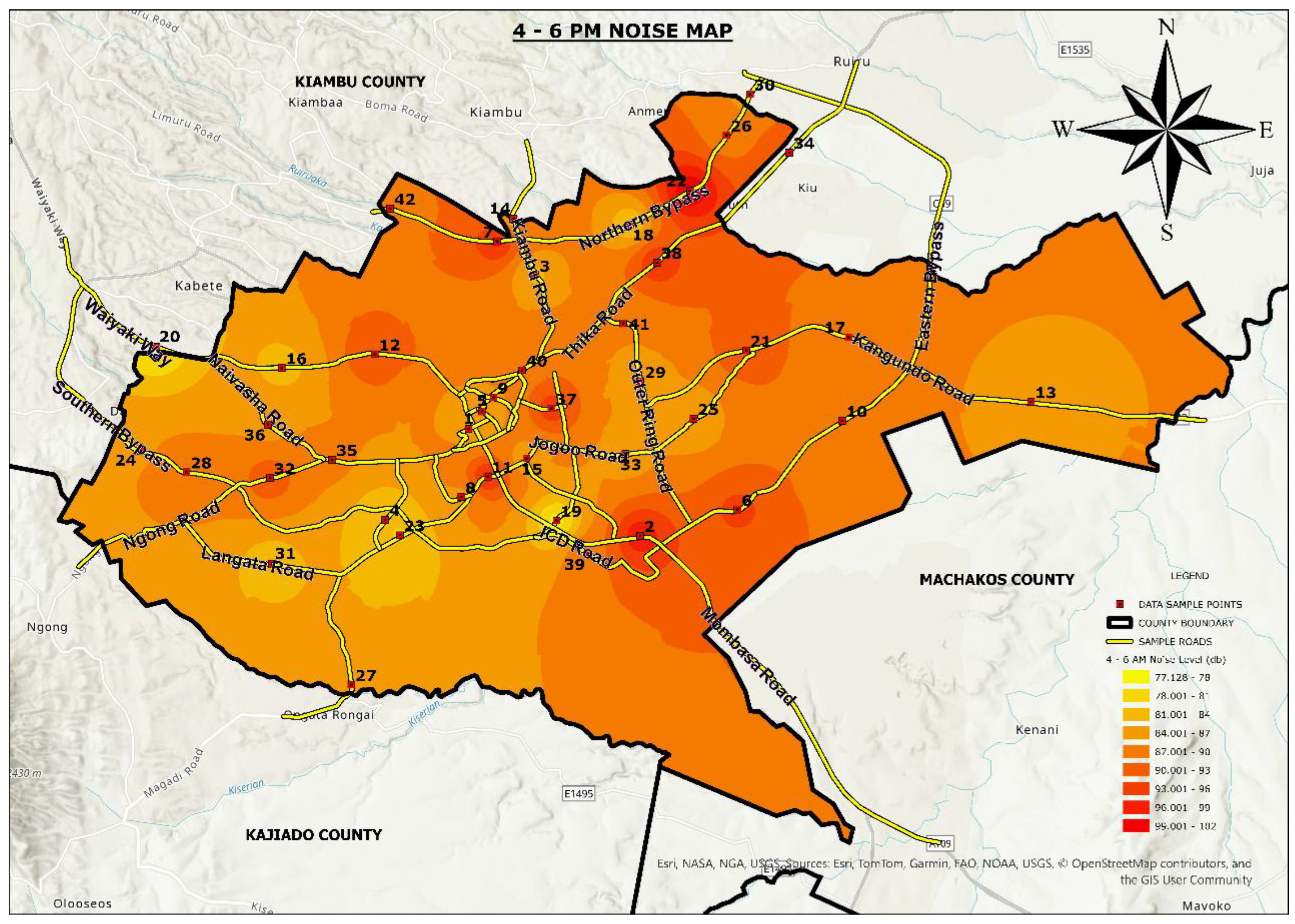
Application of the Inverse Distance Weighting (IDW) interpolation in ArcGIS produced six high-resolution spatial models of RTN levels, representing the different time bands, see Figure 7, Figure 8, Figure 9, Figure 10, Figure 11 and Figure 12.
The interpolated noise surface revealed distinct spatial gradients, with the highest noise levels consistently observed at sites located along major traffic corridors, including Thika Superhighway, Mombasa Road, Uhuru Highway, Waiyaki Way, and Jogoo Road. The IDW interpolation’s smooth gradient surfaces depicted the influence of traffic volume and road hierarchy on spatial noise distribution, with notable hotspots around high-density intersections and roundabouts. These findings confirm the efficacy of the IDW approach for representing urban noise fields and underscore its potential as a decision-support tool for targeted mitigation strategies, zoning enforcement, and proactive urban soundscape planning in Nairobi.
4. Discussion
From the results, early morning, from 6 AM to 8 AM, averaged a Leq of approximately 75.3 dBA across all sites. This can be attributed to fewer vehicles on the road, which allows drivers to move at relatively high speeds, generating elevated noise levels, despite the lower traffic volume. Levels were lowest between 8 AM–10 AM, approximately 74.5 dB(A), due to heavy traffic flow during morning rush hour. A smaller peak occurred from 10 AM to 12 PM, approximately 77.6 dB(A), likely due to reduced traffic volume and steady vehicle movement. Values were highest between 12 PM–2 PM, approximately 79.1 dB(A). This is due to less vehicular activity during lunch hour, but increased speed on the roads. In the afternoon, levels were approximately 76.0 dB(A) from 2 PM to 4 PM due to slightly lower traffic volumes, though the continuous presence of vehicles such as motorcycles, public service Vehicles (PSVs), among others, sustains moderate noise levels. Noise levels dropped slightly to approximately 74.9 dB(A) from 4 PM to 6 PM, representing evening rush hour when high traffic density, congestion, and frequent horn use combine. All values exceeded the World Health Organization (WHO) recommended limit of 55 dB(A) for residential areas and Kenya’s NEMA 50 dB(A) threshold for mixed residential–commercial zones.
The spatial distribution of Road Traffic Noise levels across Nairobi revealed distinct patterns that align with land use, traffic density, and road hierarchy. The noise maps generated illustrate a concentration of high noise across major roads. Some commercial areas, such as the Central Business District and Eastleigh, revealed persistent high noise exposure throughout the day. This can be attributed to the mixed traffic activity and frequent honking. Also, roads such as Thika Road, Ngong Road, Mombasa Road, and Northern bypass were observed to be major noise hotspots. In contrast, some residential areas like Karen and Runda recorded comparatively lower Leq values, although they are still above NEMA and WHO limits. These findings highlight that even relatively quiet suburbs in Nairobi experience chronic noise exposure. Areas with less vehicular volume, such as ICD Road, also experience high RTN levels. This can be attributed to the high levels of speeds of moving vehicles. The mapping results provide actionable insights beyond temporal trends alone and reveal major noise hotspots in the city, such as areas along Thika Road, Waiyaki Way, and in Eastleigh, among others. By visualizing the geographic extent of city-wide RTN, authorities can develop and implement noise mitigation and abatement strategies and policies. Urban residents are also able to identify habitable areas with tolerable RTN levels.
5. Conclusion
This study shows the importance of integrating GIS-based spatial mapping into Road Traffic Noise (RTN) assessment, providing practical benefits that extend beyond simply tracking changes over time. It provides a powerful means of visualizing the distribution of high-exposure areas, enabling city authorities to employ targeted interventions and enforcement efforts, and urban residents to choose suitable residential areas based on their level of RTN tolerance. Furthermore, the spatial patterns revealed in this study highlight the value of GIS-based predictive models in forecasting future noise conditions under varying scenarios of urban expansion and transportation development. These capabilities make mapping a critical tool for informed, proactive noise management in Nairobi.
This work was carried out in collaboration among all authors. Author OAE designed the study, performed the all the analysis, wrote the first draft of the manuscript. Authors OSN and GJF proof read the draft. All authors read and approved the final manuscript.
Authors have declared that they have no known competing financial interests or nonfinancial interests or personal relationships that could have appeared to influence the work reported in this paper.
Author(s) hereby declare that NO generative AI technologies such as Large Language Models (ChatGPT, COPILOT, etc.) and text-to-image generators have been used during the writing or editing of this manuscript.
Appendix 1
Table showing the RTN levels across different time bands.
| Place | X-Coord | Y-Coord | 6 AM-8 AM | 8 AM-10 AM | 10 AM-12 PM | 12 PM-2 PM | 2 PM-4 PM | 4 PM-6 PM |
| 1 | 256896.83 | 9857588.15 | 72.82 | 71.62 | 73.67 | 74.57 | 71.67 | 71.07 |
| 2 | 264136.81 | 9853108.54 | 82.14 | 80.99 | 83.04 | 83.79 | 80.99 | 80.34 |
| 3 | 259705.60 | 9864042.77 | 75.19 | 74.09 | 76.14 | 76.84 | 74.74 | 73.49 |
| 4 | 253374.75 | 9853775.07 | 71.5 | 71.3 | 73.35 | 74.05 | 71.35 | 70.65 |
| 5 | 257452.84 | 9858326.03 | 74.9 | 75.15 | 76.9 | 77.9 | 75.2 | 74.6 |
| 6 | 268248.56 | 9854218.08 | 82.07 | 82.02 | 84.07 | 84.77 | 82.07 | 81.47 |
| 7 | 258096.36 | 9865454.82 | 78.21 | 78.56 | 80.61 | 81.31 | 78.61 | 78.01 |
| 8 | 256590.06 | 9854730.41 | 77.65 | 78 | 80.05 | 80.75 | 78 | 77.35 |
| 9 | 257947.14 | 9858910.23 | 73.42 | 73.32 | 75.37 | 76.07 | 73.32 | 72.77 |
| 10 | 272667.35 | 9857939.17 | 77.69 | 76.79 | 78.84 | 79.54 | 76.79 | 76.24 |
| 11 | 258094.93 | 9867236.88 | 76.81 | 75.81 | 77.86 | 78.56 | 75.81 | 75.26 |
| 12 | 257702.58 | 9855591.69 | 79.64 | 78.79 | 80.84 | 81.54 | 78.84 | 78.24 |
| 13 | 252935.73 | 9860718.79 | 80.02 | 79.17 | 81.22 | 81.92 | 79.22 | 78.62 |
| 14 | 280644.38 | 9858744.19 | 75.05 | 74.2 | 76.25 | 76.95 | 74.25 | 73.65 |
| 15 | 258775.95 | 9866407.85 | 74.2 | 73.35 | 75.4 | 76.1 | 73.4 | 72.7 |
| 16 | 259340.90 | 9856361.23 | 74.69 | 73.84 | 75.89 | 76.59 | 73.84 | 73.29 |
| 17 | 249008.64 | 9860131.61 | 70.39 | 67.99 | 73.29 | 77.24 | 71.99 | 70.54 |
| 18 | 272942.89 | 9861441.77 | 74.64 | 74.09 | 75.64 | 76.89 | 74.44 | 73.64 |
| 19 | 263693.17 | 9866165.94 | 71.83 | 70.68 | 74.18 | 75.43 | 71.78 | 70.78 |
| 20 | 260611.02 | 9853750.71 | 67.81 | 66.91 | 71.21 | 73.71 | 69.51 | 67.56 |
| 21 | 243719.36 | 9861018.07 | 68.21 | 66.81 | 71.76 | 75.26 | 70.06 | 67.91 |
| 22 | 268614.18 | 9860885.34 | 72.38 | 71.63 | 74.63 | 75.38 | 72.68 | 71.63 |
| 23 | 266227.84 | 9867581.20 | 79.91 | 78.96 | 83.11 | 84.91 | 81.71 | 80.16 |
| 24 | 253993.82 | 9853130.38 | 71.95 | 71.1 | 75.2 | 77.15 | 73.9 | 72.4 |
| 25 | 243042.87 | 9856654.09 | 73.39 | 72.54 | 76.54 | 78.625 | 75.54 | 74.44 |
| 26 | 266390.05 | 9858026.26 | 69.32 | 68.47 | 72.42 | 74.52 | 71.57 | 70.07 |
| 27 | 267772.27 | 9869917.36 | 71.9 | 70.8 | 74.85 | 76.85 | 74.2 | 71.8 |
| 28 | 251958.55 | 9846860.37 | 70.61 | 69.46 | 73.31 | 75.41 | 72.56 | 70.51 |
| 29 | 244992.07 | 9855764.76 | 75.89 | 75.04 | 78.69 | 80.99 | 78.29 | 76.39 |
| 30 | 264131.37 | 9859591.32 | 73.43 | 72.58 | 76.23 | 78.53 | 75.47 | 74.48 |
| 31 | 268760.56 | 9871638.60 | 74.43 | 73.58 | 77.23 | 79.53 | 75.99 | 75.03 |
| 32 | 248613.98 | 9851927.16 | 68.73 | 67.88 | 71.53 | 73.83 | 70.98 | 69.53 |
| 33 | 248517.89 | 9855522.13 | 79.65 | 78.8 | 82.7 | 84.75 | 81.885 | 80.4 |
| 34 | 263515.43 | 9856549.12 | 73.6 | 72.8 | 75.95 | 77.75 | 74.475 | 73.1 |
| 35 | 270432.25 | 9869181.99 | 82.63 | 81.68 | 85.08 | 87.38 | 83.18 | 81.93 |
| 36 | 251145.89 | 9856292.64 | 75.49 | 74.64 | 78.34 | 80.69 | 76.49 | 75.34 |
| 37 | 248423.11 | 9857765.12 | 76.13 | 75.28 | 78.98 | 81.33 | 76.83 | 75.78 |
| 38 | 260390.54 | 9858451.41 | 80.59 | 79.74 | 83.79 | 85.79 | 82.89 | 81.39 |
| 39 | 264838.81 | 9864569.18 | 82.65 | 81.4 | 85.1 | 87.45 | 84.55 | 83.45 |
| 40 | 261941.98 | 9852338.53 | 76.91 | 75.71 | 79.36 | 81.66 | 78.46 | 77.05 |
| 41 | 259152.23 | 9860048.07 | 77.36 | 76.51 | 80.41 | 82.46 | 78.51 | 77.16 |
| 42 | 263418.15 | 9862017.95 | 76.02 | 75.17 | 78.82 | 81.12 | 77.42 | 76.72 |
References
- Arseni, M., Voiculescu, M., Georgescu, L. P., Iticescu, C., & Rosu, A. (2019). Testing different interpolation methods based on single beam echosounder river surveying: Case study—Siret River. ISPRS International Journal of Geo-Information, 8(11), 507. [CrossRef]
- Bartier, P. (1996). Multivariate interpolation to incorporate thematic surface data using inverse distance weighting (IDW. Computers & Geosciences. [CrossRef]
- Basner, M., Babisch, W., Davis, A., Brink, M., Clark, C., Janssen, S., and Stansfeld, S. (2014). Auditory and non-auditory effects of noise on health. The Lancet, 383(9925), 1325–1332. [CrossRef]
- Bélisle, E., Huang, Z., Le Digabel, S., and Gheribi, A. (2015). Evaluation of machine learning interpolation techniques for prediction of physical properties. Computational Materials Science, 98, 162–172. [CrossRef]
- Bhunia, G. S., Shit, P. K., & Maiti, R. (2018). Comparison of GIS-based interpolation methods for spatial distribution of soil organic carbon (SOC). Journal of the Saudi Society of Agricultural Sciences, 17, 114–126. [CrossRef]
- Boumpoulis, V., Michalopoulou, M., & Depountis, N. (2023). Comparison between different spatial interpolation methods for the development of sediment distribution maps in coastal areas. Earth Science Informatics, 16, 1–19. [CrossRef]
- Dey, J., Laxmi, V., Kalawapudi, K., Singh, T., Vijay, R., Motghare, V. M., and Kumar, R. (2021). Strategic noise mapping of Mumbai city, India: A GIS-based approach. Applied Acoustics, 48, 202–212.
- Esmeray, E., and Eren, S. (2021). GIS-based mapping and assessment of noise pollution in Safranbolu, Karabuk, Turkey. Environment, Development and Sustainability, 23(10), 15413–15431. [CrossRef]
- Garg, N., Sinha, A., Dahiya, M., Gandhi, V., Bhardwaj, R., & Akolkar, A. (2017). Evaluation and analysis of environmental noise pollution in seven major cities of India. Archives of Acoustics, 42(2), 175–188. [CrossRef]
- İlgürel, N., Akdağ, N., and Akdağ, A. (2016). Evaluation of noise exposure before and after noise barriers: A simulation study in Istanbul. Journal of Environmental Engineering and Landscape Management, 24(4), 293–302. [CrossRef]
- İmamoglu, M. Z., & Sertel, E. (2016). Analysis of different interpolation methods for soil moisture mapping using field measurements and remotely sensed data. International Journal of Environment and Geoinformatics, 3(3), 11–25.
- Islam, R., Sultana, A., Reja, M. S., Seddique, A. A., & Hossain, M. R. (2024). Multidimensional analysis of road traffic noise and probable public health hazards in Barisal city corporation, Bangladesh. Heliyon, 10(15), e35161. [CrossRef]
- Jalilzadeh, R. (2007). Evaluation of noise pollution using GIS: Case study of the 9th district of Tehran, Iran. Proceedings of the MapAsia 2007 Conference, Kuala Lumpur, Malaysia, August 14–16.
- Morillas, J. M. B., Escobar, V. G., Sierra, J. A. M., Vílchez-Gómez, R., and Trujillo Carmona, J. (2002). An environmental noise study in the city of Cáceres, Spain. Applied Acoustics, 63(10), 1061–1070. [CrossRef]
- Münzel, T., Schmidt, F. P., Steven, S., Herzog, J., Daiber, A., & Sørensen, M. (2018). Environmental noise and the cardiovascular system. Journal of the American College of Cardiology, 71(6), 688-697. [CrossRef]
- Münzel, T., Sørensen, M., Gori, T., Schmidt, F. P., Rao, X., Brook, F. R., Chen, L. C., Brook, R. D., and Rajagopalan, S. (2017). Environmental stressors and cardio-metabolic disease: Part II—Mechanistic insights. European Heart Journal, 38(8), 557–564. [CrossRef]
- Murphy, E., and King, E. (2014). Environmental noise pollution: Noise mapping, public health, and policy. Elsevier. [CrossRef]
- Murphy, E., and King, E. A. (2010). Strategic environmental noise mapping: Methodological issues concerning the implementation of the EU Environmental Noise Directive and their policy implications. Environment International, 36(3), 290–298. [CrossRef]
- Ozer, S., Yilmaz, H., Yesil, M., & Yesil, P. (2009). Evaluation of noise pollution caused by vehicles in the city of Tokat, Turkey. Scientific research and essay, 4(11), 1205-1212.
- Partheeban, P., Krishnamurthy, K., Partheeban, N. E., Krishnan, S., and Baskaran, A. (2022). Urban road traffic noise on human exposure assessment using geospatial technology. Environmental Engineering Research, 27(5), 210249. [CrossRef]
- Pathak, V., Tripathi, B. D., and Mishra, V. K. (2008). Evaluation of traffic noise pollution and attitudes of exposed individuals in working place. Atmospheric Environment, 42(16), 3892–3898. [CrossRef]
- Singh Upendrasingh R., Shivendra Kumar Jha, (2023) Integrating GIS in Road Traffic Noise Assessment: A Review of Methods and Applications. Journal of Neonatal Surgery, 12, 74-78.
- Thanh, B. P. P., & Hạnh, N. T. X. (2021). Mapping and distribution of noise using IDW interpolation algorithm in Thuan An city, Binh Duong province. Thu Dau Mot University Journal of Science, 3(4), 64–76. [CrossRef]
- Ware, C., Knight, W., & Wells, D. (1991). Memory intensive statistical algorithms for multibeam bathymetric data. Computers & Geosciences, 17(7), 985-993. [CrossRef]
- Wawa, E. A., & Mulaku, G. C. (2015). Noise pollution mapping using GIS in Nairobi, Kenya. Journal of Geographic Information System, 7(5), 486-493. [CrossRef]
- Zafar, M. I., Dubey, R., Bharadwaj, S., Kumar, A., Paswan, K. K., Srivastava, A., ... & Biswas, S. (2023). GIS based road traffic noise mapping and assessment of health hazards for a developing urban intersection. In Acoustics (Vol. 5, No. 1, pp. 87-119). MDPI. [CrossRef]
- Zhou, Z., Zhang, M., Gao, X., Gao, J., & Kang, J. (2024). Analysis of traffic noise spatial distribution characteristics and influencing factors in high-density cities. Applied Acoustics, 217, 109838. [CrossRef]
Figure 1.
Map showing Nairobi City, Kenya (Source; Author).
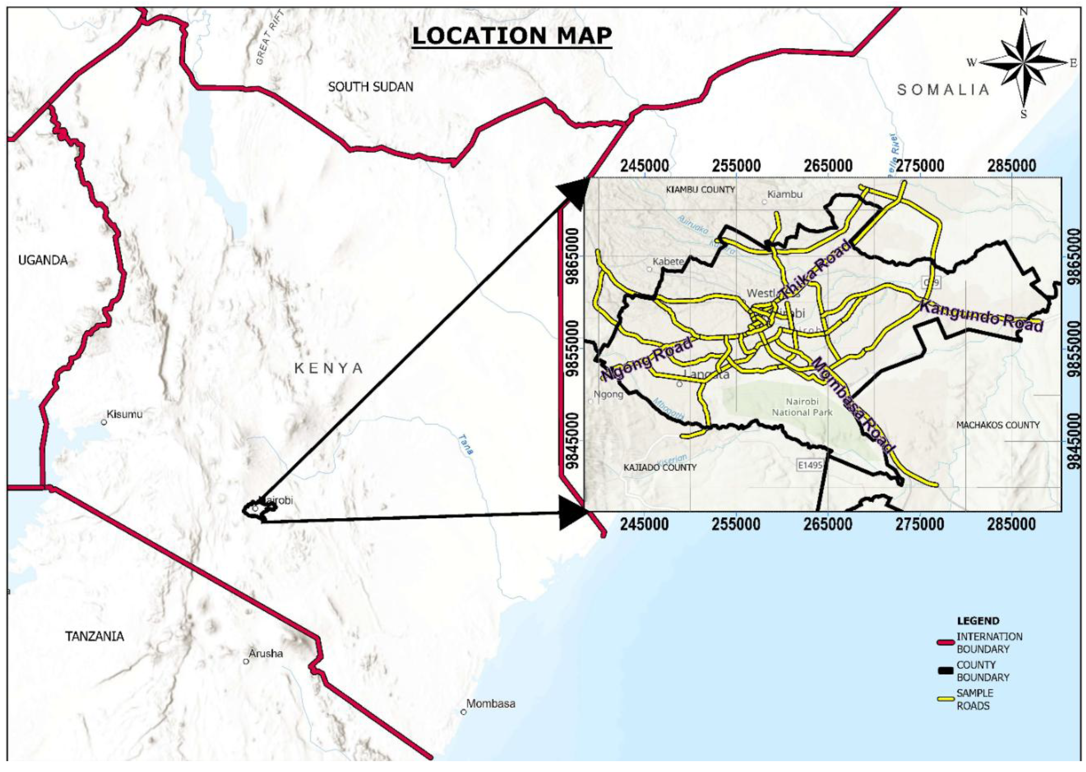
Figure 2.
Map of the 42 Sampling points across Nairobi City (Source; Author).
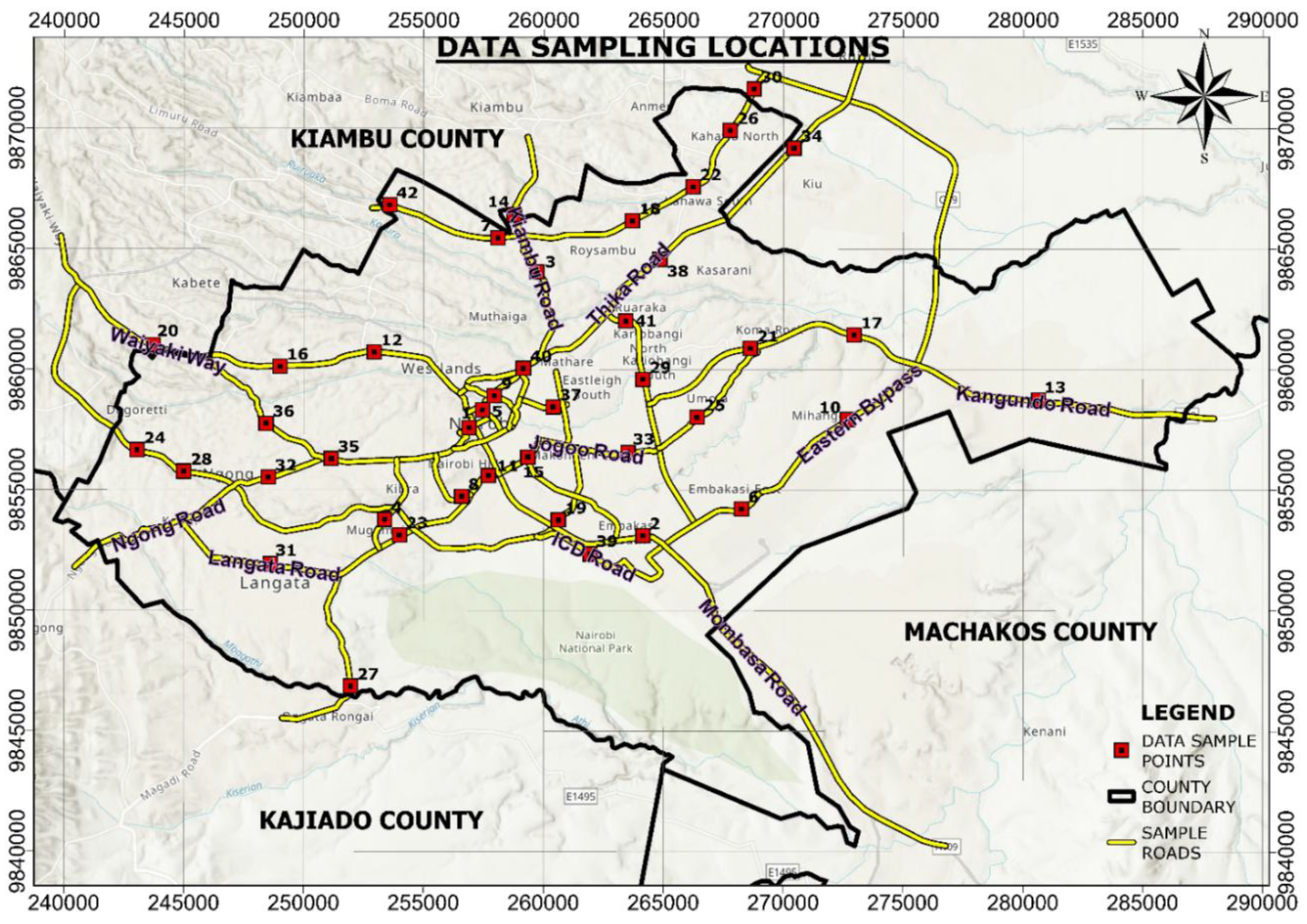
Figure 1.
Sound Level Meter (Source: author).
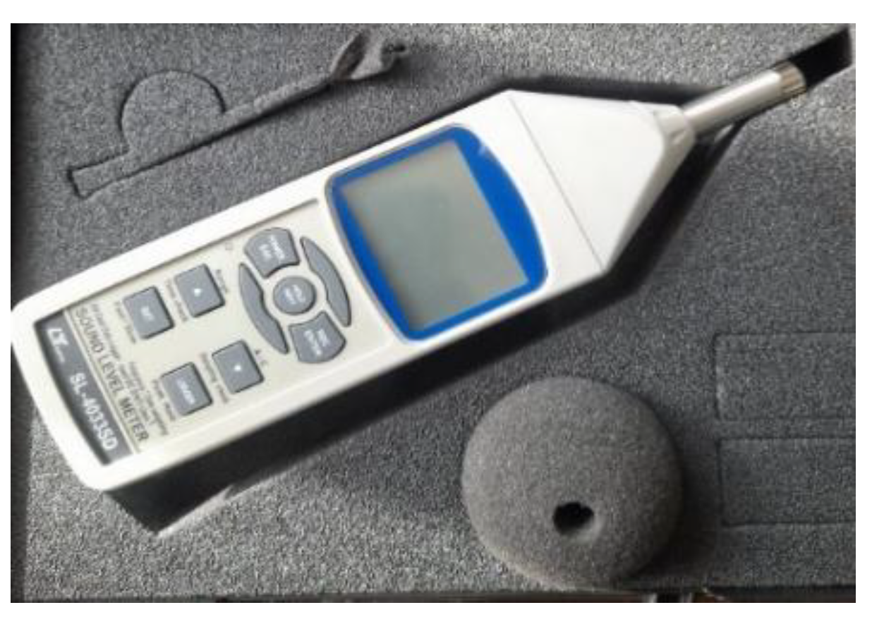
Figure 4.
Data Collection along Kiambu Road (Source: author).
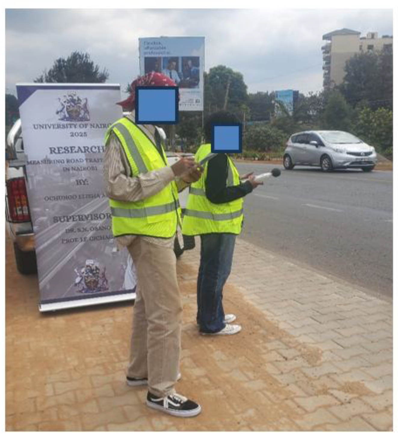
Figure 5.
conceptual workflow chart presented (Source: Author).
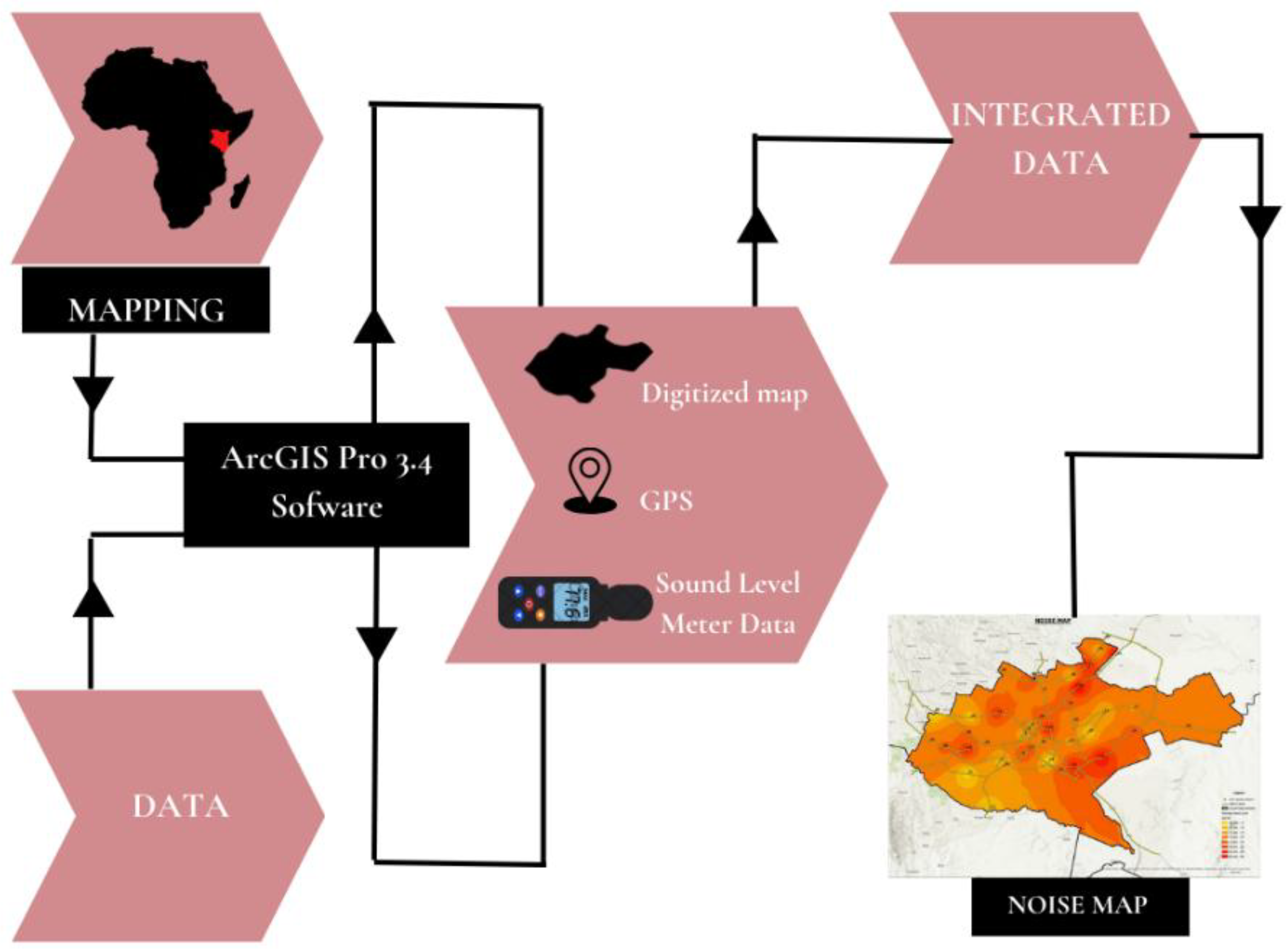
Figure 6.
Average RTN levels in Nairobi City across different time bands.
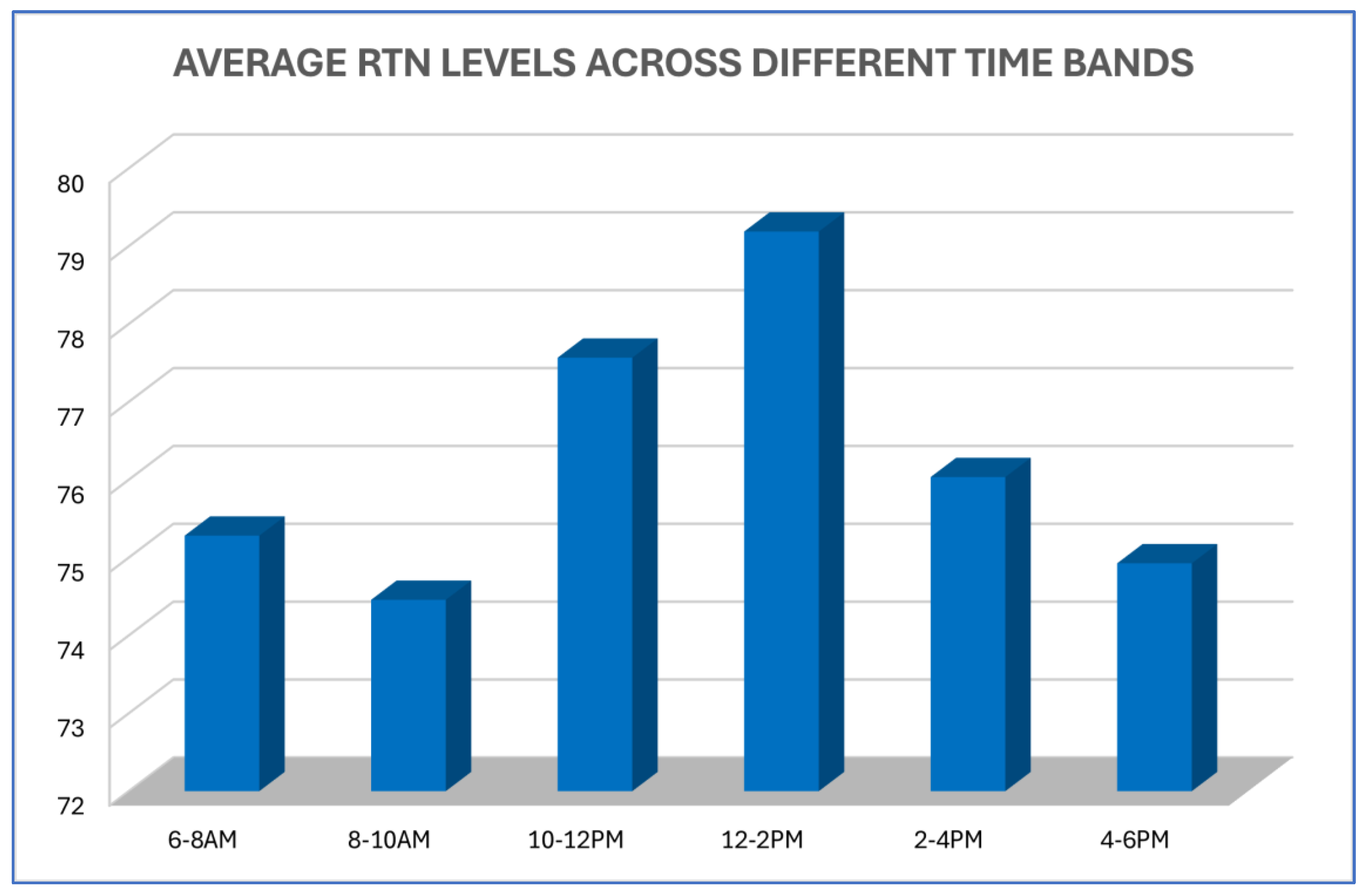
Figure 7.
Noise map showing RTN levels 6 AM-8 AM.
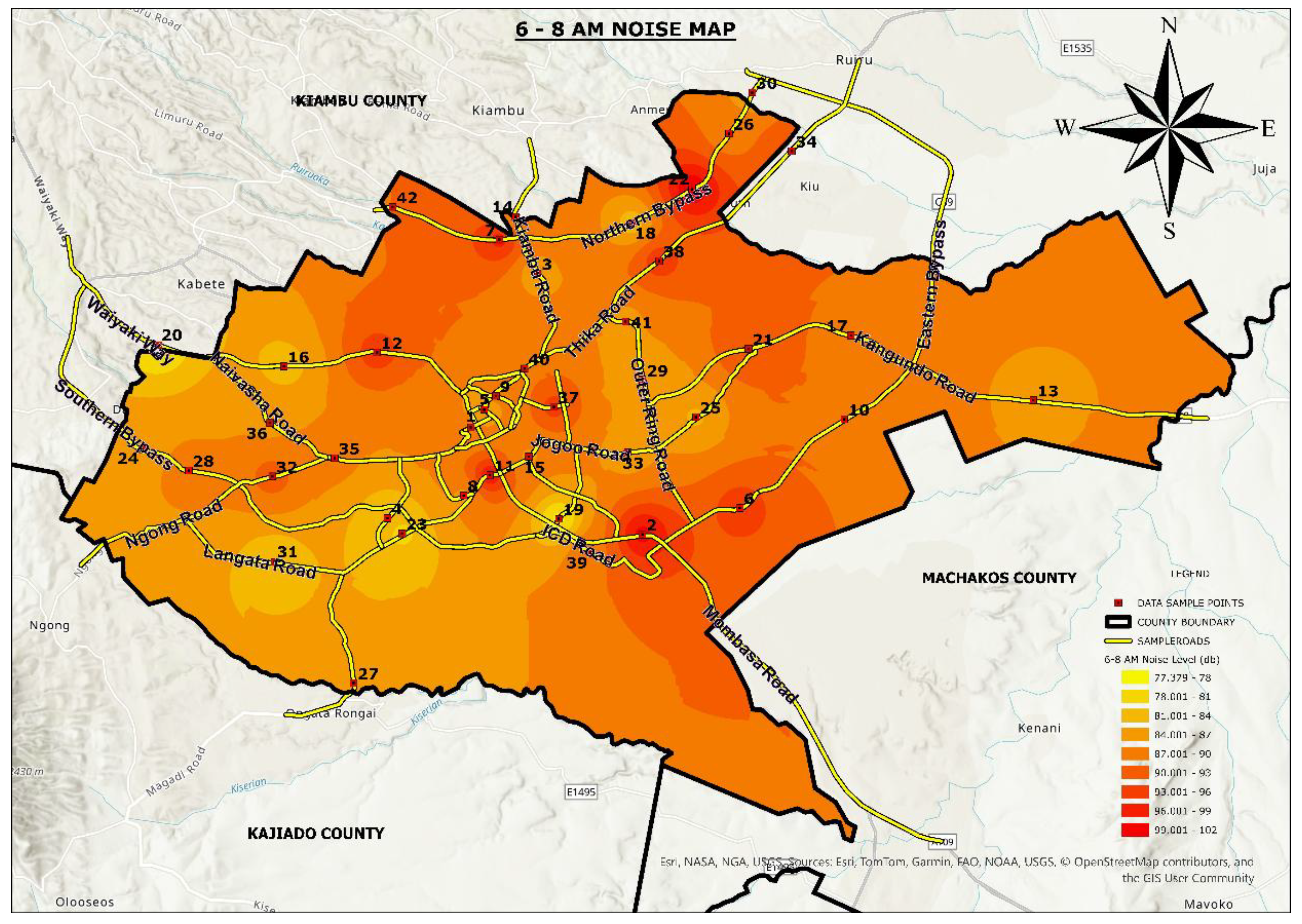
Figure 8.
Noise map showing RTN levels 8 AM-10 AM.
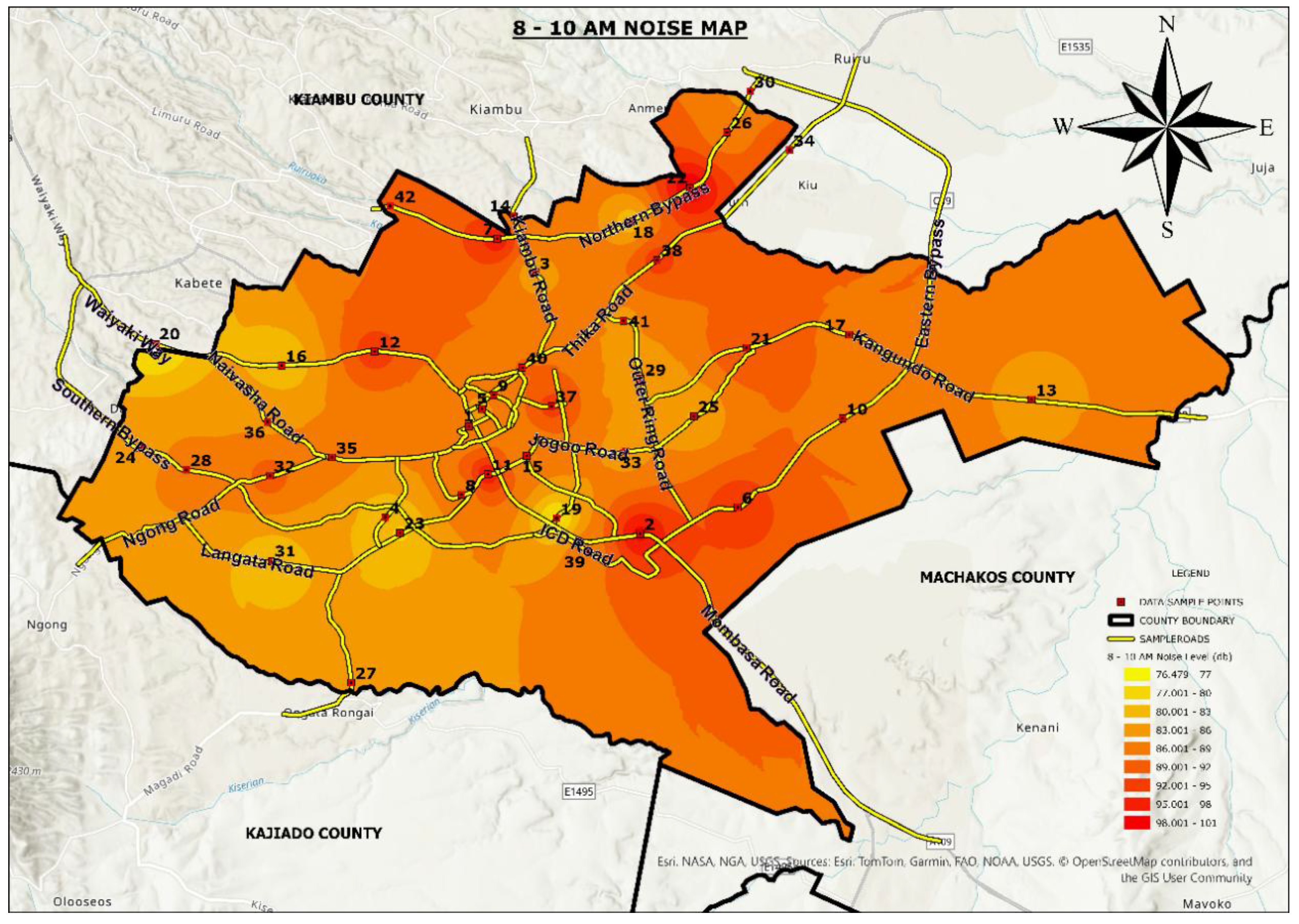
Figure 9.
Noise map showing RTN levels 10 AM-12 PM.
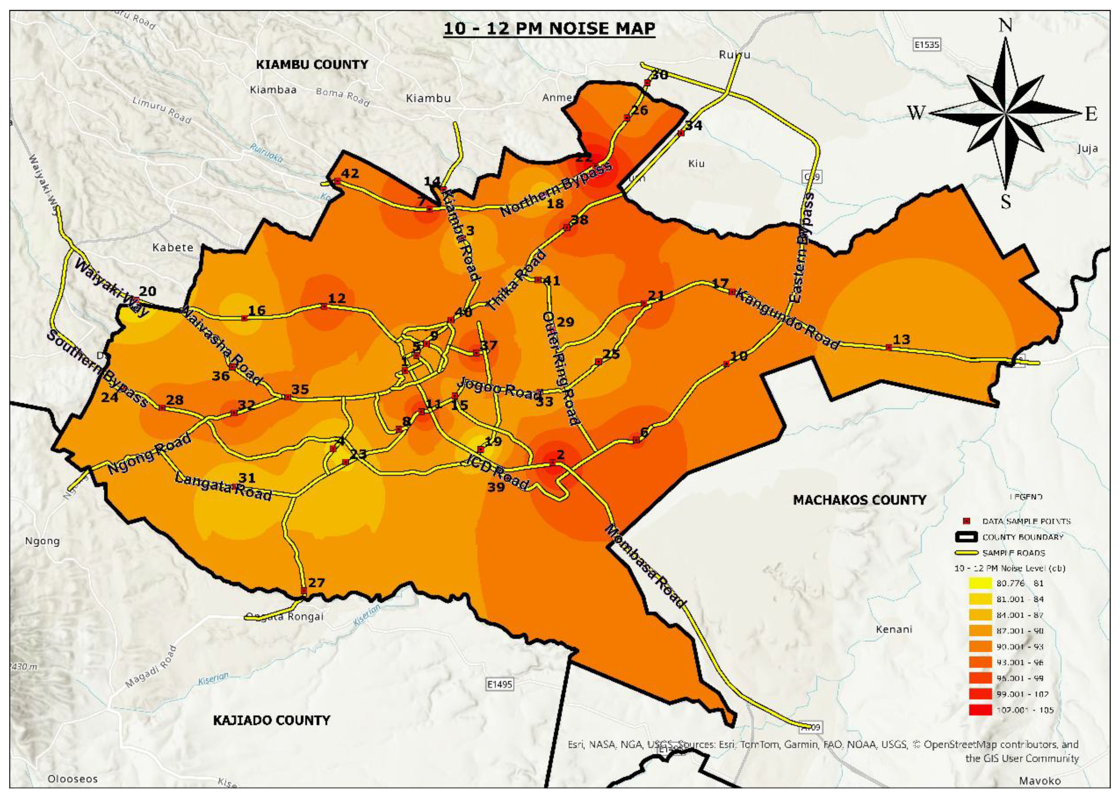
Figure 10.
Noise map showing RTN levels 12 PM-2 PM.
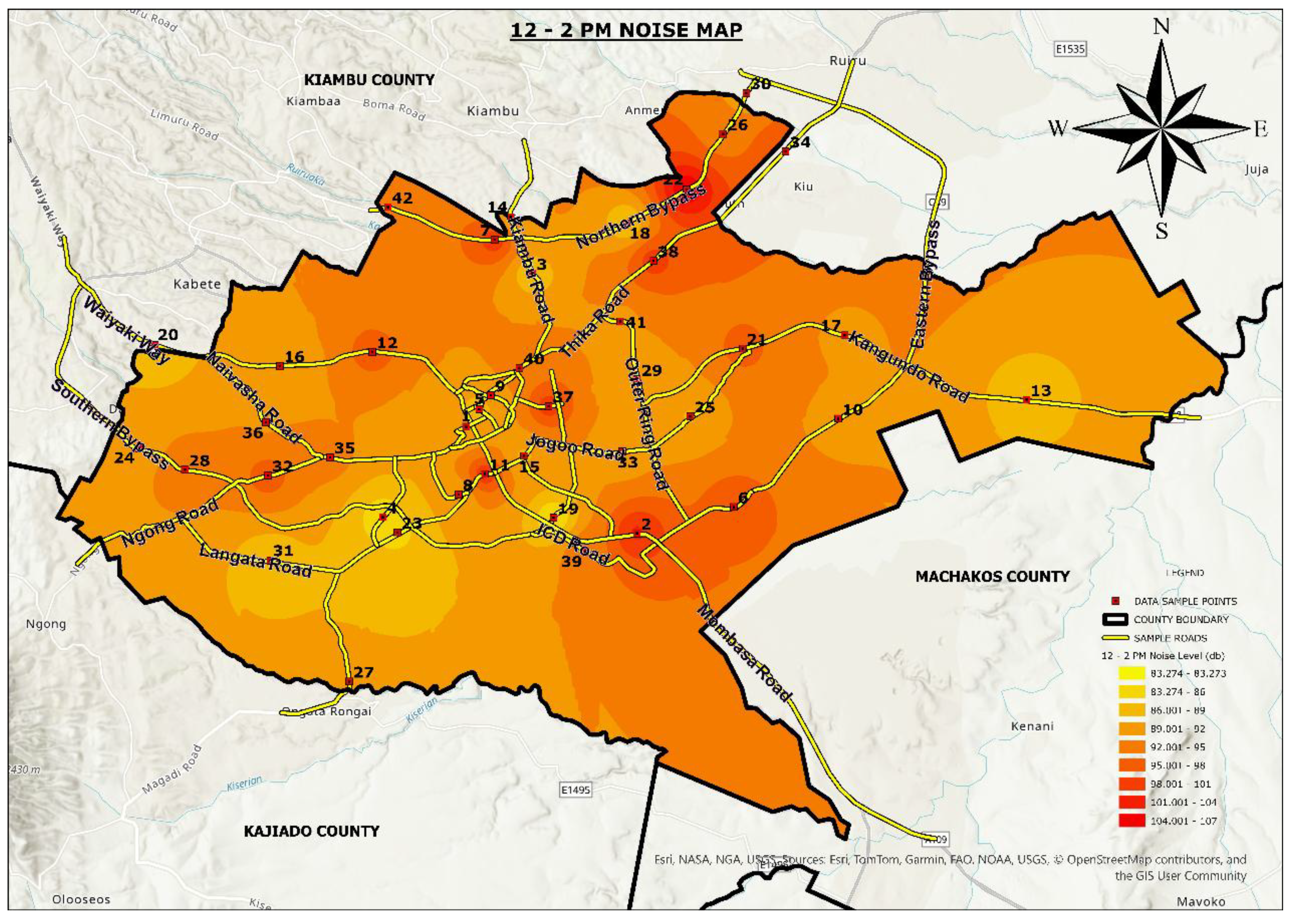
Figure 11.
Noise map showing RTN levels 2 PM-4 PM.
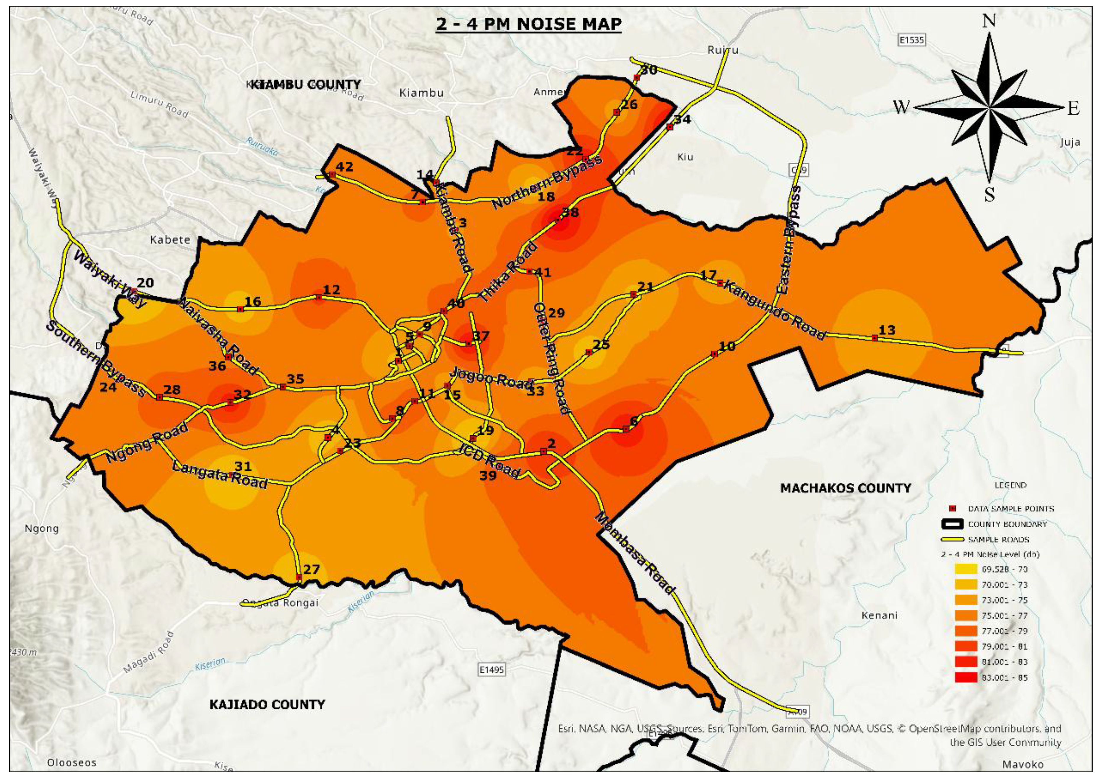
Figure 12.
Noise map showing RTN levels 4 PM-6 PM.
Disclaimer/Publisher’s Note: The statements, opinions and data contained in all publications are solely those of the individual author(s) and contributor(s) and not of MDPI and/or the editor(s). MDPI and/or the editor(s) disclaim responsibility for any injury to people or property resulting from any ideas, methods, instructions or products referred to in the content. |
© 2025 by the authors. Licensee MDPI, Basel, Switzerland. This article is an open access article distributed under the terms and conditions of the Creative Commons Attribution (CC BY) license (http://creativecommons.org/licenses/by/4.0/).
Copyright: This open access article is published under a Creative Commons CC BY 4.0 license, which permit the free download, distribution, and reuse, provided that the author and preprint are cited in any reuse.


